Abstract
The aim of this study is to analyze the dynamics of the housing market in Turkey’s economy and to examine the impact of variables related to housing prices. Preferred by many international housing investors, Turkey hosts profitable real estate investments as one of the developing countries with a shining housing market. This study applies the dynamic model averaging (DMA) methodology to predict monthly house price growth. With the increasing use of information technologies, Google online searches are incorporated into the study. For this purpose, twelve independent variables, with the Residential Property Price Index as the dependent variable, were used in the period January 2010–December 2019. According to the analysis results, it was observed that some variables, such as bond yields, the level of mortgages, foreign direct investments, unemployment, industrial production, exchange rates, and Google Trends index, are determinants of the Residential Property Price Index.
1. Introduction
Housing, an important subbranch of the real estate market, is an important part of the sustainable economy. In several countries having one’s own real estate property is perceived as having a high social status and is the aim of young people entering the job market. On the other hand, the housing market attracts investors, who perceive real estate not only as a consumption good, but also as an asset in which money can be allocated (Gebeşoğlu 2019).
Although their intentions are different, the parties who want to buy houses enter the real estate market and may benefit from increases in a property’s value. Property value is related directly to the housing ownership ratio. Especially in developing countries, whether the high rate of housing ownership is sustainable is discussed in the literature. The main question of the sustainability of the housing market is affordability. Housing cannot be sustainable unless it is low-priced and cost-effective. Whether housing is cost-effective also affects the sustainability of its use as an investment tool (Nuuter et al. 2014; Wang et al. 2012). The real estate market is more stable than volatile financial markets such as foreign exchanges, interest rates, and the stock market. In the real estate sector, which has become a very profitable investment tool, especially in the last 15 years1, housing prices determine the profitability of the sector. At this point, the determination of housing prices has been one of the most important subtopics of the sector. This topic has prompted many market players, from residential investors to real estate investment trusts and from individual investors to government officials, to predict the movement of housing prices, and they use a variety of methods for this (Gupta et al. 2011; Ghysels et al. 2013; Yemelina et al. 2018; Kishor and Marfatia 2018).
The development of new housing price prediction models would greatly assist in the prediction of future housing prices and the establishment of real estate policies. This paper implements dynamic model averaging (DMA), a new technique, to predict the movement of housing prices. DMA is gaining increasing attention in macroeconomic time series forecasting due to its ability to accommodate time variation in both the parameters as well as the specification of the optimal forecasting model (Yusupova et al. 2019). In addition to giving better results with macro variables, one of the advantages of the DMA method is that it allows the parameters and prediction model to change over time. One other distinguishing feature of DMA is that the method captures not only parameter shifts, but also model changes (Bork and Moller 2015; Wei and Cao 2017). A scarcity of studies using the DMA technique in other topics connected with finance and economics in the literature has been observed. This study contributes to the existing literature by allowing the estimation of housing prices with a new technique (DMA) using macroeconomic data. Moreover, the lack of an application of DMA to the Turkish housing market, which constitutes the sample of this study, and the advantages of the model are the main motivations for this study. It is also worth mentioning that, in the case of housing prices analysis, DMA has significant prediction gains compared to a linear autoregressive (AR) model, offering a series of predictions that compete with competitive dynamic and static prediction models (Yusupova et al. 2019). The dynamic averaging scheme allows us to obtain the probability that each variable is included over time. This feature was found to be appropriate in this study as the most functional method that can be used to understand the driving forces of each housing market and to see and demonstrate the behavior they exhibit over time.
Housing prices can provide important information to stakeholders in the real estate market, including real estate agents, appraisers, assessors, mortgage lenders, brokers, property developers, investors and fund managers, and policy makers, as well as to actual and potential homeowners. It is difficult to accurately estimate housing prices. The reason for this is that residences are generally a combination of various factors such as location, environment, and structural features (Bin 2004). It is not clear how to select the factors involved and how these factors will be taken into account.
In the evaluation of house prices, the use of the RPPI, which measures the change in the price of houses as a percentage from a certain starting date, is considered. It is also considered that the housing market demand and supply amounts, the general economic conditions affecting the sale and purchase of housing, the movements in the financial market, and the real sector factors affecting commercial life should be included in the study. Consumers’ perceptions of housing purchases and their reactions to prices through online searches will also be explored.
With the increasing use of information technologies, online searches have become one of the important factors that have been increasingly used in academic articles in recent years (Shimshoni et al. 2009; Ginsberg et al. 2009; Choi and Varian 2012). Internet online searches also play a role in housing pricing in the real estate sector (Ford et al. 2005; Kulkarni et al. 2009; Hohenstatt et al. 2011; Beracha and Wintoki 2013; Das et al. 2015; Wei and Cao 2017). Moving from this point, one of the distinguishing features of this study is combining the DMA method with the Google Trends index, following Wei and Cao (2017).
As seen from different DMA studies (Raftery et al. 2010; Aye et al. 2015; Bork and Moller 2015; Risse and Kern 2016; Wei and Cao 2017; Sousa 2018; Yusupova et al. 2019), it is clear that the DMA model is generally applied for the analysis of datasets from developing countries. Turkey is considered a developing country, and the application of this method in Turkey is another contribution to the literature.
Increased real estate development over the last 15 years has brought Turkey more to the attention of international housing investors. The decisive role of the sector, especially in the economic recession, has caused greater interest in the behavior of the real estate markets. Foreigners showed an increase in development of 78% compared to the previous year, buying about 40,000 housing units in 2018 in Turkey (AREREIT 2019b). The lack of focus on research mainly on the Turkish real estate market is another motivation for this study.
This paper is structured as follows: The next section provides a review of the real estate market and then provides theoretical background and information on the Turkish real estate market. In the third section, relevant literature is reviewed; the fourth section gives details about the sample selection and the methodology used. In the last section, results are discussed and conclusions are formulated.
1.1. Why Housing? Why Housing Prices?
The spread of the 2008 mortgage crisis from the United States to the whole world caused all countries to become more interested in the real estate sector. (The 1997 Asian crisis and the boom in asset prices before the 1929 and 2008 crises in the United States are examples of major financial crises that can be caused by speculative housing price bubbles.) The importance of monitoring the price movements and loan amounts of the housing sector became clear after the 2008 global financial crisis, and since that time, its importance has only increased. Monitoring housing prices, which both reflect developments in the housing market and provide information about the housing market’s connection to other macroeconomic variables, has enabled both autonomous and state institutions to follow the housing sector much more closely. Long-term increases in housing prices, together with excessive investment, can lead to speculative price movements, which are called bubbles and have negative effects on sustainable economic growth (Beltratti and Morana 2010). Considering their impact on other sectors of the economy, analysis of housing prices becomes even more important.
The fact that housing directly and indirectly affects financial stability has made it mandatory to follow the housing market and home prices (Uyar and Yayla 2016). The housing market is one of the leading drivers of the economy due to its forward and backward effects in both developed and developing countries. Especially for the economic stability of developing countries, resource allocation is becoming even more important. Developments in the housing market can play a decisive role in long-term sustainable economic growth, potentially affecting the allocation of resources used in production (Hongyu et al. 2002). Excessive investment in the housing market can delay resource allocation and prevent sufficient investment in areas such as education, industry, and high technology necessary for sustainable growth. Consequently, developing countries are experiencing serious financing problems. In other words, the limited productivity of housing investment compared to other types of investment, and yet excessive investment in housing, can lead to less investment in areas that are much more productive and vital for sustainable development.
Housing expenditures have a significant weight in total expenditures. For this reason, housing is related to many macroeconomic variables, including GDP, price indices, interest rate, and investment (Bilik and Aydin 2019). The construction sector, which provides employment for many people, is directly related to the housing market and affects important economic data such as labor force participation and unemployment, increasing the importance of the housing sector in the economies of a country.
While housing is considered an alternative to securities in some cases, in others it is considered a high-profit investment tool. For this reason, it differs from other markets. The high cost of housing supply, permanent housing, maintaining stable housing (as a long-term investment), heterogeneous growth in secondary markets, and use of collateral in financial transactions can be listed as differences between other markets and the housing market (Afşar et al. 2017). For example, house prices in the Turkish economy have increased more than 230% since 2003 according to the REIDIN House Price Index, and consumer prices have increased at a much more severe rate than agricultural and industrial prices, giving investors very high returns (Yıldırım 2017). In addition, when analyzed, it has the advantage that nominal housing prices do not fall as sharply as stock and commercial real estate prices. Therefore, investors tend to buy more houses. On the other hand, housing investments in Turkey constitute more than half of the net wealth of the private sector (Arslan and Kasa 2020). The low return performances of real sector (agricultural, industrial, etc.) investments and financial investment instruments compared to the housing sector should be investigated. One of the primary motivations for this study is the relatively small amount of literature on housing price prediction compared to agricultural, industrial, and financial assets such as stock prices and exchange rates.
Another dimension of housing prices is housing expenditures. Expenditures for housing, which are sometimes seen as a consumption good and an investment good by households, have an important share in total expenditures. Again, to give an example from Turkey, in the last 15 years, approximately 27% of household consumption expenditures are allocated to housing and rent expenditures, and these expenditures are the highest share of household consumption expenditures (Kolcu and Yamak 2018).
Another aspect of the issue is that the housing market is related to the socioeconomic structure of countries. Turkey has a young population structure; continued urbanization due to internal migration; continued external growth from different countries, especially neighboring countries; increased housing purchases by foreigners; and a downsizing Turkish family structure, and all indicate that long-term housing demand will increase in Turkey (Bilik and Aydin 2019).
Based on this crucial importance of the housing market, the prediction of housing prices is also important in that it provides information to all interested parties.
1.2. Theoretical Background
The main link between real estate price determination and basic macro variables stems from the credit growth trend approach. Since the purchase of homes is financed through the banking system, greater financial depth and accelerated loan growth rate tend to increase housing demand, possibly by increasing property prices. This situation is called the house prices channel in theory (Mishkin 2001). The house prices channel can be defined as the process of changing the total output and price level by a change in monetary policy affecting real estate prices, such as housing and land, and thus the investments and expenditures of the household. High interest rates increase household savings and narrow the demand for investment-oriented housing. However, when interest rates fall, home prices increase. An increase in house prices increases consumption and investments through wealth and collateral effects. As a result, total demand increases.
The Modigliani consumption life cycle model is effective in the functioning of the house prices channel. In this transfer mechanism, direct effects, such as capital use cost effect and interest rates and wealth effect, and indirect effects, such as housing and rental wealth and collateral, affect the investments or expenditures of firms or households. Changes in investments and expenditures change the total output amount (Milcheva and Sebastian 2010). Wealth effects impact consumption decisions, while collateral effects impact investment decisions. When house prices increase, the net wealth of the household increases, increasing consumption and, consequently, positively influencing economic activity. The opposite happens when house prices fall: consumption decreases as a result of wealth effects, and economic activity decreases.
Housing prices, which affect economic activity, can directly affect the loan demand of the real estate sector, which can be used as collateral for mortgage financing in the housing and loan markets. When housing prices change, the loan demand of both households and commercial enterprises can change and affect their investments. Housing investment is considered an indicator of healthy functioning in economies and an important part of the total investment. Sari et al. (2007) stated that housing market activity is important for the economy because the increase in housing investments increases employment in the housing construction sector and related industries that provide housing-related goods and services. Workers' income increases in the housing sector and industries that supply goods and services to the housing sector, and the increase in income tends to increase the demand for housing with its multiplier effect. As a result, employment is assumed to be one of the leading indicators of future housing investment.
Banks are willing to ensure the availability of home loans or mortgages in order to avoid the decline in their capital, which might be determined by the decline in real estate prices in the market. Friedman and Kuttner (1993) argue that when loans from credit institutions decrease, investors enter the stock market. Sudden increases and decreases in the value of assets such as securities and treasury bills, on the other hand, affect the interest rates and cause fluctuations in the total loan supply. When regular interest rates go up, the mortgage rate or mortgage payment (including interest and principal) increases and prevents people from buying houses, so the demand for houses decreases.
Case et al. (2005) show that changes in real house prices can even impact consumption more strongly than changes in stock market prices, which might be due to the fact that house ownership is more evenly distributed across households than stock market wealth. In contrast, stock market wealth is mainly held by rich households. Since the propensity to consume declines with increasing wealth, an increase in house prices should therefore have a stronger effect on consumption than an increase in stock prices. Some economists, however, do not believe in the existence of such wealth effects (Adams and Füss 2010).
One of the biggest problems of developing countries (including Turkey) is the current account deficit and foreign capital inflows used in financing the deficit and the related exchange rate volatility. When the increase in exchange rates arises from capital movements, it causes continuous current account deficits and poses a risk. The very short duration of capital inflows and high domestic inflation compared to the outside world are the main reasons that cause the excessive appreciation in exchange rates (Karadaş and Salihoglu 2020). Due to the effect of rising house prices on consumption and imports, an increase in foreign currency demand can be seen.
At the same time, inflationary effects in developing countries can cause changes in exchange rates, which can affect house prices and cause price changes. In such countries, it is assumed that housing demand will increase when the housing loan interest rates and inflation rates decrease. However, in Turkey, contrary to expectations, when housing prices increase, housing sales increase rather than decrease. Therefore, it is expected that both market dynamics and credit trends are important in real estate price prediction, and it is necessary to first investigate which should be dominant.
1.3. Why Turkey?
We have some interesting reasons for choosing Turkey as a sample. First, the housing sector in Turkey is important for both domestic and foreign investors. The great development in the real estate sector in Turkey over the last 15 years has garnered more attention from international housing investors. The decisive role of the sector, especially in the economic recession, has caused great interest in the behavior of the real estate markets. Foreign investment showed an increase of 78% compared to the previous year, buying about 40,000 housing units in 2018 from Turkey (AREREIT 2019a). Housing sales to foreigners, as of the end of the first quarter of 2020, increased to 10,948 units with a growth of 13.8% compared to the same period of the previous year (see Figure 1) (AREREIT 2020b). According to balance of payment data, gross foreign direct investment (FDI) into Turkey stood in the region of USD 8.8 billion for the first 11 months of 2019, of which USD 4.5 billion was gross real estate acquisition investments (AREREIT 2020a).
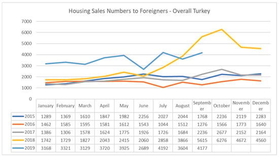
Figure 1.
Housing sales numbers to foreigners—overall Turkey (source: AREREIT 2020a, 2020b) This table shows housing sales to foreigners. Turkey stands out as a center of attraction for investment in housing for foreigners. Sales to foreigners in the third quarter of 2018 broke a record, and they remained flat until the third quarter of 2019.
Growth potential in the domestic market in recent years, coupled with an expected increase in real estate value, has led to growing foreign investor interest in the Turkish real estate market. Factors such as legal regulations facilitating the acquisition of property by foreigners in Turkey, large-scale residential projects, and the phenomenon of migration-driven demand have also had a positive impact on investment in the sector (AREREIT 2020a). On the other hand, in a country like Turkey, where foreign financing needs are high, the purchasing of houses by foreign investors has a positive effect on the balance sheet in the form of direct foreign capital. For example, approximately 25% (USD 24,708 billion) of a total direct capital inflow of USD 97,257 billion in the 2011–2017 period was realized as real estate purchases (JLL 2020). It would be appropriate to investigate the method of covering this financing need with the sale of housing on a long-term basis.
Real housing prices in the world, in general, have been on an upward trend since 1990. Especially after the 2001 crisis, the increase in national income per capita thanks to economic growth on the one hand and the restructuring of the banking and financial system through a series of reforms on the other have led to the revival of the housing sector in the Turkish economy. This revival went into decline with the 2008 crisis but has risen again since 2012. The rise in home prices in the Turkish economy over the mentioned period has outstripped most of the United States, Eurozone, Canada, United Kingdom, and other developed countries (Yıldırım 2017). Istanbul, Turkey’s largest and most important city, is shown as the seventh most attractive residential market in Europe after London, Paris, Moscow, Milan, and Rome. Additionally, Turkey is recognized as the best performing residential market in the world, with an 18.4% price increase, ahead of New Zealand, Australia, and Sweden (JLL 2020). Therefore, this situation makes the Turkish economy, which is the sample of our study, an extremely important field of research in terms of explaining the rapid rise in housing prices in the world.
Another core motivation for the study is the increasing interest in the real estate sector in Turkey because it is one of the sectors that are most open to development in Turkey. The legendary growth rate of 64.9% in 2013 was followed by growth rates of 10.4% in 2015, 4.0% in 2016, and 5.1% in 2017 (AREREIT 2019a). In 2018, with 1,375,398 housing units, 2.4% growth in the real estate sector, net direct international investment inflows of approximately USD 13 billion are observed (AREREIT 2019c). In 2019, 1,348,729 housing units, compared to 2018, represented a decline of 1.9%. Based on December 2019 figures, at over 200,000, house sales for Turkey as a whole broke an all-time record (AREREIT 2020a). This interest in the real estate sector also brought real estate investment trusts with it. The number of real estate investment companies (REITs), which were very few in the early 1990s, reached 33 by the end of 2018, especially as a result of the intensive investments and significant incentives made to the construction sector in recent years. As a result of these figures, real estate in Turkey reached the point of becoming a USD 400 billion sector. These statistics indicate the importance of predicting real estate prices (AREREIT 2019c).
The housing sector gained momentum after mortgage regulations made great progress. Mortgage sales, which have become an important point to be watched carefully both in terms of the sector and the economy, have started to affect macro data. In 2019, Turkey’s mortgaged sales recovered to record a 20.1% increase over the previous year (AREREIT 2020a). As of the first quarter of 2019 and the same period of 2020, mortgage sales increased by 90%. During this period, a decrease in interest rates and its effect on credit costs have positively affected mortgage sales, which seems to have a positive effect on the economy (AREREIT 2020b). In other aspects, the growth rate of bank loans, in which the ever-increasing housing loans have an important place in Turkey, is quite high. According to Dalkılıç and Aşkın (2018), Turkey ranks third among 44 countries studied in terms of loan growth. Forty percent of the personal loans provided consist of housing loans. Credit institutions prefer to allocate housing loans more because they do not have any problems in collecting the housing loans they provide.
Another reason for Turkey to be chosen as the sample is its high need for housing. When we look at the home ownership rate of countries in the period of 2007–2017, Turkey comes after Germany and Austria with a home ownership rate of approximately 60% (Alp 2019). The increase in the rate of home ownership is associated with the increase in welfare in the society, an increase in wealth and fair distribution of wealth, and increases in total consumption and economic growth due to the increase in wealth. In addition, there are various indications that some of the participants in the housing market in Turkey conduct their home purchases and sales with nonconsumption incentives, such as accumulating wealth and investing beyond their own housing need. The short return period of the housing investment has a great effect on this (Alp 2019). High inflation and insufficient efficiency of the capital market are also counted in buying and selling housing for investment purposes (Coskun 2016).
When the first quarter of 2019 and the same period of 2020 are analyzed, there has been an increase of 3.4% in total house sales. The 119% increase in second-hand sales during the mentioned period indicates that residences in the market are in demand (AREREIT 2020b). The Turkish construction and housing sector will continue to be one of the economic drivers of Turkey. When the demographic and economic developments are taken into consideration and compared with the world, it will be seen that the housing sector contains more potential than other sectors of the economy. Therefore, as the stability and the dynamic structure of the Turkish housing sector continue, the trend will be towards growth in the medium and long term.
In Turkey, due to the high rate of housing ownership and high housing production costs and therefore housing prices, the determinants of housing prices in terms of economic stability and sustainable economic growth are worth investigating.
2. Literature Review
In the monetary policy transmission mechanism, the important role of housing markets and housing investments affects and shapes many macroeconomic variables. Housing investments in Turkey, which constitute the sample of this study, represent more than half of the net wealth of the private sector (Arslan and Kasa 2020). This figure shows how big the housing demand is in the market. The effects of housing demand on the housing market and the general economy arise in relation to housing prices. In this context, the increase/decrease effects of the changes in housing supply and demand on housing prices may affect the actual debt burden, potential return, potential/current consumption, and savings flows of the mortgage loan holders. On the other hand, changes in housing prices affect the volumes of credit/securitization institutions and their risks related to these transactions on the macro level (Coskun 2016). In the context of the global financial crisis, especially in countries where the housing–finance bond is strong, such as Turkey, it has been revealed that monitoring changes in housing prices as a key indicator of the housing market is important for understanding the risk accumulations in the overall economy.
Housing prices are an issue that attracts both researchers and the public. The first studies of housing prices date back to the 1960s. The ideas that Lancaster (1966a, 1966b) put forward as consumer theory later evolved into the hedonic pricing model, for which Rosen (1974) formed the theoretical basis. Harrison and Rubinfeld (1978) then Li and Brown (1980) investigated housing prices using hedonic methods. Hedonic housing prediction (Stadelmann 2010; Liu 2013; Fotheringham et al. 2015; Nicholls 2019; Liu et al. 2020; Li et al. 2021) has remained popular, although various techniques have been applied with developing econometric methods. In time series, cointegration analyses (Zhang et al. 2012; Al-Masum and Lee 2019; Stevenson and Young 2014), impact response analyses (Fry et al. 2010), error correction method (Shi et al. 2021), and causality tests (Kulkarni et al. 2009; Su et al. 2019) have continued to be used. Panel data analyses (Adams and Füss 2010; Hadavandi et al. 2011; Wu and Brynjolfsson 2015; Glaeser and Nathanson 2017) are also used to measure the movement of house prices. In the last few years, the dynamic model averaging (DMA) model has been implemented, which gives better results with macro data (Wei and Cao 2017).
The use of DMA for housing price prediction began with Bork and Moller (2015) in the United States. Another of the first studies that used the DMA method, this time among different countries, is the work of Risse and Kern (2016) that applied it to the six largest countries of the European Monetary Union between the years 1975 and 2015. Afterward, Yusupova et al. (2019) developed the adaptive dynamic model averaging (ADMA) methodology, stating that DMA is important in macroeconomic time series prediction due to its ability to accommodate both the time variability in parameters and the specification of the optimal prediction model. In their work with the United Kingdom’s regional house price indices from 1982 to 2017, the authors claimed that better prediction results could be obtained through the ADMA methodology.
Sousa (2018) presented another study applying the DMA methodology to predict quarterly house price growth in Portugal, Spain, Italy, Ireland, the Eurozone, and the United States. Despite the increasing globalization of economies and financial markets, the author concluded that each individual housing market is subject to its own dynamics. In another application of DMA in the real estate sector, Akinsomi et al. (2016) attempted to predict the growth rates of U.S. real estate investment trusts (REIT) from January 1991 to December 2014. They found that indicators, monetary policy instruments, and sensitivity indicators across the economy are among the strongest determinants of REIT returns.
In another DMA study, Wei and Cao (2017) studied the growth rate of housing prices for 30 major cities in China. The authors used the Google Trends index as an additional determinant beyond traditional economic variables to predict changes in Chinese house prices. In recent years, the Google Trends index has been found to develop higher predictive success for housing prices in China than key macroeconomic or monetary indicators.
One of the originalities of this study is the combination of the DMA method and the Google Trends index. With increasing information technologies becoming more ubiquitous, online searches have become increasingly inevitable in academic articles. Internet information research on products and housing in the real estate sector also plays a critical role in pricing. In this regard, Das et al. (2015) examined the relationship between online flat rental searches and basic real estate market variables, vacancy rates, rental rates, and real estate asset price returns. The authors found that consumer real estate Internet searches were significantly correlated with market fundamentals after checking the known determinants of these variables. Another study in this direction is the research by Beracha and Wintoki (2013), which found that abnormal Internet search intensity for real estate in a given city could help predict future abnormal house price changes in the city.
The literature review shows that academics have turned to OECD countries and developing countries to predict house prices. Aizenman and Jinjarak (2014) investigated the real estate valuation before and after the 2008–2009 crisis in a panel of 36 countries by introducing the crisis range. They found that there has been a strong positive relationship between real estate valuation and increases in current account deficits and credit growth rates in those countries covering the OECD and emerging markets. Anundsen et al. (2016) examined house prices and credit growth for 20 OECD countries between 1975 and 2014. They found that bursts of credit to both households and nonfinancial companies affected the stability of the financial system. Confirming previous studies, Paul (2018) highlighted that rapid rises in housing prices are strong early warning indicators of financial crises and their severity. In another study in 2019, Paul (2019) said that the response of housing prices is strongly in line with the level of housing prices. He found that when house prices are high, they react less to monetary policy shocks, but when prices are low, they are more sensitive to monetary policy shocks. He emphasized that bubble-like behaviors in housing prices are harbingers of crises. These studies have revealed the necessity of investigating house prices in Turkey, an OECD country and a developing country that has experienced many financial crises. This study is focused on investigating the house price dynamics of Turkey and revealing its macroeconomic dimensions, as in other developing country examples, which simultaneously fills a gap in the literature on this issue.
Although providing better results with macro data on predictions of housing prices, a study by the DMA implementation in Turkey could not be identified. In Turkey, hedonic pricing model (Yayar and Gül 2014; Kördiş et al. 2014; Daşkiran 2015; Güler et al. 2019), artificial neural network method (Yılmazel et al. 2018), cointegration analysis (Sağlam and Abdioğlu 2020), and causality test (Akkaş and Sayılgan 2015) techniques have been used. In most of the studies on housing prices in Turkey, it was observed that local house prices were investigated on a provincial basis rather than on a country basis (Yayar and Gül 2014; Kördiş et al. 2014; Daşkiran 2015; Yılmazel et al. 2018; İslamoğlu and Nazlıoğlu 2019; Güler et al. 2019). Another striking feature in the studies is the investigation primarily of the reflections of house features on prices (Yayar and Gül 2014; Kördiş et al. 2014; Yılmazel et al. 2018; Güler et al. 2019). Another point that inspires this study is that there are few studies for the prediction of house prices with macro variables (Akkaş and Sayılgan 2015; Gebeşoğlu 2019; İslamoğlu and Nazlıoğlu 2019).
Meanwhile, in the literature, it is expected that both inflation rates and housing interest rates would affect the valuation of national real estate. However, Berry and Dalton (2004) emphasize that interest rate, investment demand, and the current economic environment affect housing prices, which they characterize as short-term factors. On the contrary, Luo et al. (2007) state that the behavior of home buyers is influenced by recent market information. Thus, they claim that house prices are raised by the expectations of people rather than their income. While Sirmans et al. (2005) divided these factors into eight categories, we will simply examine them under the headings of macroeconomic, financial, and housing market dynamics. Our regressors include macroeconomic factors (inflation rates, unemployment rate, Industrial Production Index, foreign direct investments), financial factors (the difference between bond yields, stock price indices, exchange rates), and housing market factors (Residential Property Price Index, home loan interest rates, mortgage amounts, the number of dwellings) as key indicators that have been studied extensively in the literature.
While investigating the relationship between the real estate sector and the indicators of countries, inflation rates (Fry et al. 2010; Aizenman and Jinjarak 2014; Risse and Kern 2016; Wei and Cao 2017; Yusupova et al. 2019; Paul 2019) draw attention as the top macro variable that affects the housing prices. Home loan interest rates (Arsenault et al. 2013; Aizenman and Jinjarak 2014; Risse and Kern 2016; Wei and Cao 2017; Sousa 2018; Al-Masum and Lee 2019) and the difference between bond yields (Arsenault et al. 2013; Aizenman and Jinjarak 2014; Bork and Moller 2015; Risse and Kern 2016; Wei and Cao 2017; Sousa 2018; Paul 2019; Yusupova et al. 2019; Shi et al. 2021) are important factors that are found to shape the house prices in the studies. Unemployment rates (Bork and Moller 2015; Wei and Cao 2017; Sousa 2018; Al-Masum and Lee 2019; Yusupova et al. 2019), Industrial Production Index (Aizenman and Jinjarak 2014; Bork and Moller 2015; Risse and Kern 2016; Wei and Cao 2017; Paul 2019; Yusupova et al. 2019), and foreign direct investments (Aizenman and Jinjarak 2014; Chow and Xie 2016; Guest and Rohde 2017) stand out as the most widely used economic indicator variables in the literature when investigating housing prices of countries. To measure the impact of financial markets on housing prices, stock price indices (Fry et al. 2010; Aizenman and Jinjarak 2014; Risse and Kern 2016; Paul 2019) and exchange rates (Fry et al. 2010; Risse and Kern 2016; Gebeşoğlu 2019) are the most prominent macro variables. In the literature, housing demand is generally measured by mortgage amounts (Arsenault et al. 2013; Aizenman and Jinjarak 2014; Yusupova et al. 2019; Shi et al. 2021), while the number of dwellings (Sousa 2018; Al-Masum and Lee 2019; Shi et al. 2021) is used to measure the amount of housing supply. In studies, it is noted that Residential Property Price Index (RPPI) (Fry et al. 2010; Aizenman and Jinjarak 2014; Bork and Moller 2015; Risse and Kern 2016; Wei and Cao 2017; Sousa 2018; Al-Masum and Lee 2019; Shi et al. 2021) represents housing prices.
As a result of this literature review, the main purpose of this study is to predict the right housing prices, to find the right method to catch the right variables and the right clues, and to reach the most accurate results in the right country by using the available technological facilities. Combining the macro variables and Google search results with the DMA method, this study on the Turkish market contributes to the literature by providing valuable information about the business cycle of the housing sector in order to help governments and policymakers better regulate the real estate market. To do so, it aims to reveal the factors affecting the real economy.
3. Data
The analyzed period covers the time span between January 2010 and December 2019. Monthly data were taken. House prices were measured by the Residential Property Price Index (RPPI), which is published by the Turkish Central Bank (2020). This index is constructed on a countrywide basis and includes data from the biggest cities. It excludes from computations any city with an insufficient number of observations.
The selection is also in line with, for example, the work of Wei and Cao (2017). The level of mortgages (housing finance with loans from banks and financing companies) in thousands of TRY was taken as an indicator of demand (mortgage). The number of two or more dwelling residential buildings was taken as an indicator of supply (dwellings). Residential buildings with two or more dwellings including apartments and multiflat buildings. These data have been obtained from TURKSTAT by CBRT according to construction statistics and building occupancy permits. The Consumer Price Index (cpi), measuring the inflation level, was also considered. For measuring economic growth and economic conditions, foreign direct investment (FDI) in real estate activities was considered (fdi). As an indicator of interest rates, the interest rate for housing was taken (i_rate). The unemployment rate was denoted by u_rate. The economic conditions were also measured by Industrial Production Index (ipi). Stock prices were measured by Borsa Istanbul 100 Index (stocks). The exchange rates were measured by USD/TRY (usd) and EUR/TRY (eur). The interest rate spread was measured as the difference between the 10-year Turkish bond yield and 2-year bond yield (ird). Finally, the consumers’ change in interest was measured by Google Trends index for the search query “ev fiyatları” meaning “house prices” (gt). Google Trends is a website by Google that analyzes the popularity of top search queries in Google Search across various regions and languages (Google 2020). The website uses graphs and datasets to compare the search volume of different queries over time. Table 1 reports the variables used in the research.

Table 1.
Variable description table.
The data were collected from the Turkish Central Bank (2020), Stooq (2020), and Google (2020).
The variables RPPI, mortgage, cpi, stocks, usd, and eur were transformed into logarithmic differences. In particular, if yt is the time series to be transformed, then its logarithmic difference is log(yt)–log(yt−1). Following, for example, Koop and Korobilis (2013), both transformed and untransformed variables were further transformed into approximately stationary forms by standardization. In particular, if yt is the time series to be standardized, then the standardized time series is obtained as yt = (yt − μ)/σ, where μ denotes the mean and σ denotes the standard deviation of the full time-series considered. To prevent the forward-looking bias, means and standard deviations for standardization were estimated on the basis of the first three-fourths of the sample. Further on, this period constituted the in-sample, and further observations were used as pseudo-out-of-sample.
Table 2 reports the descriptive statistics for the whole sample obtained from the transformations described above. Table 3 reports the results of the stationarity tests (statistics and p-values). In particular, the augmented Dickey–Fuller test (ADF), Phillips–Perron test (PP), and Kwiatkowski–Phillips–Schmidt–Shin test (KPSS) were performed. Assuming 10% significance level, all the time series except i_rate can be assumed stationary. However, it was decided not to transform i_rate further, because of its economic interpretation and properties. Secondly, in the dynamic model averaging scheme, stationarity is not a significant obstacle towards inserting a variable into the modeling scheme (Drachal 2019a).
Table 2.
Descriptive statistics.
Table 3.
Stationarity tests.
4. Methodology
The computations were performed in R (R Core Team 2018) with the help of “fDMA”, “forecast”, “glmnet”, “MCS”, and “multDM” packages (Bernardi and Catania 2018; Drachal 2018, 2019b; Friedman et al. 2010; Hyndman and Khandakar 2008). A detailed explanation of the dynamic model averaging (DMA) scheme can be found in the original paper by Raftery et al. (2010). In order not to repeat the detailed derivation of formulas, but to keep the paper self-consistent, herein just the underlying ideas are presented.
4.1. The Modeling Scheme
Suppose that, for instance, from the literature review, there are n potentially interesting time series that might serve as explanatory variables in a linear regression model. Herein, n = 12 such variables were identified. As a result, K = 2n = 4096 different multilinear regression models can be constructed, also including the model with the intercept term only. Let us denote the time index by t, and let yt denote RPPI (after the mentioned transformations). Let be the vector of explanatory variables in the k-th multilinear model, where k = 1, …, K. As a result, the state-space model is given by the following equation:
with denoting the regression coefficients in the k-th regression model. It is assumed that the errors are normally distributed, i.e., ~N(0,Vt(k)) and ~N(0,Wt(k)).
The initial variances and covariances V0(k) and W0(k) have to be specified. Concerning the standardization and results from Table 2, it seems reasonable to set V0(k) = 1 for every k = 1, …, K and to set W0(k) as the identity matrices of the dimensions equal to the dimension of the corresponding vectors Each of these K models is estimated recursively with the Kalman filter. However, to reduce the computational burden, which can easily lead to an intractable problem, Raftery et al. (2010) proposed updating W0(k) with the forgetting procedure (Karny 2006). Indeed, the number of models K grows exponentially with the linear increase in n. The forgetting procedure requires the specification of the forgetting factor λ, which should be a number between 0 and 1. Setting λ = 1 corresponds to no forgetting and the assumption that regression coefficients are fixed in time. Smaller values correspond to the higher volatility of these coefficients.
As a result, K time-varying parameter regressions are estimated. Their performance is approximated with the help of the set of two, recursively updated, weights:
where fk(yt|Yt−1) is the predictive density of the k-th model at yt, under the assumption that the data up to time t are known, and α is the next forgetting factor. This forgetting factor corresponds to attaching more weight to the k-th model performance in recent periods than to its performance in the periods more distant in the past. For instance, α = 0.99 means that for monthly data, the observations from last quarter are given approximately 97% of weight as those from the last month. Similarly, those from the last year are given only 89%.
The proper setting of the forgetting parameters can be a subtle problem. For example, too low values might result in overfitting, whereas too high values might not capture the true volatility and switching in all K models (Baur et al. 2016). Therefore, in this research the grid of all combinations of α and λ = {1, 0.99, 0.98, …, 0.91, 0.90} were tested. Again, in order not to obtain forward-looking bias, these estimations were done for the in-sample period, i.e., based on the first three-fourths of observations. However, the DMA scheme is quite chaotic in the first periods when the scheme “learns” the data. Therefore, the forecast evaluation serving as a basis for selecting the final combination of forgetting factors was performed after excluding the first one-fourth of observations from the obtained forecasts, but the last one-fourth were still also excluded to be in line with the in-sample and pseudo-out-of-sample division mentioned before.
In Equation (1), a small constant, c = 0.001/K, is added because, during numerical estimations, it can happen that the weights would be rounded to 0. Such a small constant can prevent this, and its use was advised in the original paper by Raftery et al. (2010).
To start computations, the initial values π0|0,k have to be set. The noninformative prior requires setting π0|0,k = 1/K for every k = 1, …, K.
Finally, the DMA forecast is computed as
where is the forecast obtained by the k-th component regression model. This averaging scheme can also be used to obtain weighted average values of regression coefficients; i.e.,
However, the DMA scheme itself can be easily modified. For instance, instead of averaging, a selection procedure can be performed. The natural and common one in Bayesian econometrics is to modify Equations (3) and (4) by selecting and from the k-th model, which maximizes the weight πt|t-1,k over k = 1, …, K. In other words, the model with the highest posterior probability is chosen. This scheme is called dynamic model selection (DMS).
Barbieri and Berger (2004) noticed that in the case of model selection, focusing on the highest posterior probability is not always the optimal choice. They suggested the median probability model (MPM). For this, first, for all explanatory variables, the sum of all weights πt|t-1,k—but only of those models which contain the given explanatory variable—is computed. Next, in each period t, the model which contains exactly those variables for which this sum is greater than or equal to 0.5 is selected. If the model combination scheme consists of all possible 2n component models, then the existence of such an individual component model is guaranteed.
Another interesting modification is to keep time-varying parameter regression estimations but to drop the time-varying scheme in the estimation of weights. In other words, to keep πt|t-1,k = 1/K fixed for all k = 1, …, K and for all periods t. Herein, this is called equal-weighted averaging of time-varying parameter regression (EV-TVP).
Finally, as noticed by Raftery et al. (2010), it is remarked that setting α = 1 = λ recovers Bayesian model averaging (BMA) in a computationally efficient way. For this combination of parameters, DMS and MPM schemes are called Bayesian model selection (BMS) and Bayesian median probability model (BMPM), respectively.
4.2. Benchmark Models
The estimated models were compared for forecast accuracy measures with the auto ARIMA model (ARIMA), the no-change naïve forecast (NAÏVE), and time-varying parameter (TVP) models. Besides, LASSO regression was also used in a recursive manner, as a penalized regression method, which is also often used for feature selection purposes (Tibshirani 1996).
First of all, TVP regression is simply the DMA scheme reduced to K = 1 with only one model, i.e., k = 1, in which = [1, mortgaget, dwellingst, …, irdt] consists simply of all considered explanatory variables. The forgetting factor λ for this model was taken as the same, which was obtained for the DMA scheme, in the way described above.
The no-change (NAÏVE) forecast was obtained simply by taking .
For the auto ARIMA model, the recursive estimation proposed by Hyndman and Khandakar (2008) was taken. In this scheme, models with up to 2 lags are initially considered, resulting in some prudent variation in ARIMA specification. In the next step, lags are added or removed until there is an improvement in the Akaike information criterion. However, to have a stopping criterion, no more than 5 lags are considered.
In the case of LASSO, recursive estimations were also performed. Additionally, the “lambda” penalty coefficient was selected in each recursive step on the cross-validation basis, focusing on mean square error (Friedman et al. 2010).
All these benchmark models have, like the initial DMA and its variant schemes, the recursive property. In other words, the forecast for time t is computed only based on the information known up to time t − 1.
In the case of ARIMA and NAÏVE methods, the raw, i.e., untransformed, RPPI time series was inserted. However, all others, i.e., the DMA-based schemes, forecasted standardized logarithmic differences of the RPPI. In order to obtain consistency between the outcomes from the several models, these outcomes were finally transposed back in order to be the forecasts of the raw RPPI time series.
4.3. Forecast Accuracy Evaluation
The forecast evaluation was performed based on the last one-fourth of observations. For each of the estimated models, the root mean square error (RMSE), mean absolute error (MAE), and mean absolute scaled error (MASE) were computed. The first two measures are standard and common procedures. On the other hand, Hyndman and Koehler (2006) suggested a new measure that “relates” the absolute errors with the ones from the no-change forecast. In short, this measure has some “good” properties if the forecasted values are near 0. It penalizes both positive and negative errors equally, as well as large and small values. From the interpretational point of view, when its value is greater than 1, it indicates that the no-change forecast produces a more accurate forecast.
The obtained forecasts were also compared with the Diebold–Mariano test (Diebold and Mariano 1995). As noticed by Franses (2016), the loss function corresponding to the MASE measure fits the statistical procedures of this test.
Finally, the model confidence set (MCS) procedure of Hansen et al. (2011) was performed for all obtained forecasts. This procedure is useful when comparing several forecasts. This procedure starts with a set of forecasts from all the considered models. Then, it tests if the equal predictive accuracy (EPA) hypothesis can be rejected for this set of forecasts. If so, then the “worst” performing forecast is excluded from the set of forecasts. Then, the procedure is repeated until the EPA cannot be rejected. The significance level was assumed to be 5%. Moreover, Mariano and Preve (2012) proposed an extension of the mentioned Diebold–Mariano test for the multivariate background. Their procedure is similar to the MCS one. To report the technical details, for the MCS procedure, 5000 simulations and the “Tmax” version of the statistic were taken. For the Mariano and Preve procedure, the “Sc” version of the statistic was taken, and 12 lags were taken (due to the use of monthly data and outcomes from the Tiao–Box procedure recommended in their paper).
4.4. Additional Remarks
All models, except NAÏVE, were estimated in two versions, the first one without the inclusion of the gt variable and the second one with the inclusion of the gt variable as an explanatory variable. This was done in order to compare if the Internet search queries can, indeed, be helpful in improving forecast accuracy.
Secondly, in the original paper, Raftery et al. (2010) updated variances Vt(k) with the recursive moment estimator. For example, Koop and Korobilis (2011) suggested that the exponentially weighted moving average method can be more suitable for financial time series if heteroskedasticity in errors can occur. This method requires the parameter κ to be selected. Following them, due to the use of monthly data, κ = 0.97 was taken.
5. Results
The prelimary simulations based on the first three-fourths of observations indicated that out of the considered grid of forgetting factors, the MASE measure is minimized for the following combination: α = 0.97 and λ = 0.90. As a result, this combination was used for further estimations of the models.
The results of forecast accuracy measures from the estimated models are reported in Table 4. The symbol “-GT” is added to the models containing the variable gt, i.e., the Internet search queries. It can be seen that the EV-TVP-GT model minimized all three forecast accuracy measures. It can also be seen that the DMA-based model combination schemes generally produced less accurate forecasts than those from the ARIMA models. However, the specific version, i.e., the one with averaging with equal weights, was able to produce more accurate forecasts. On the other hand, all model combination schemes were able to produce more accurate forecasts than those from the NAÏVE method. Selected forecasts are visualized in Figure A1 in Appendix A.
Table 4.
Forecast accuracy measures for the estimated models.
It is hard, however, to conclude on the basis of RMSE that adding the Internet search queries as an explanatory variable to the particular model improves its forecast accuracy. However, from considering MAE, such a conclusion is valid considering MASE leads more towards the conclusion that Internet search queries can improve the forecast accuracy.
Table 5 reports the p-values from the Diebold–Mariano test comparing forecasts from the estimated models: those with the variable gt corresponding to the Internet search queries and those without it. For each row, the null hypothesis is that forecast from the given model has the same accuracy as that from this model but with added gt variable. The alternative hypothesis is that forecast accuracies are different. Unfortunately, it cannot be concluded, even assuming some relatively high significance level, that the forecasts from the models containing the variable gt are significantly more accurate than those from the models without this variable. The Diebold–Mariano test was performed with two loss functions: squared errors (SE) and absolute scaled errors (ASE).
Table 5.
The Diebold–Mariano test (forecasts from the models with the Google Trends index for the search query variable vs. those from the models without it).
Table 6 reports the p-values from the Diebold–Mariano test comparing forecasts from the selected model EV-TVP-GT and other models. In each row, the forecast from the corresponding model is compared with the forecast from the EV-TVP-GT model. The null hypothesis of the test is that both forecasts have the same accuracy, whereas the alternative hypothesis is that the forecast from the EV-TVP-GT model is more accurate than that from the competing model. For this test, two versions were performed: one with squared errors (SE) loss function and one with absolute scaled errors (ASE).
Table 6.
The Diebold–Mariano test (forecasts from the EV-TVP-GT model vs. all other estimated models).
Assuming a 10% significance level, it can be seen that in most cases the forecast from the EV-TVP-GT model can be assumed to be statistically significantly more accurate than the forecast from the competing model. Unfortunately, this cannot be said when compared with the EV-TVP model. It also cannot be said when compared with the BMPM-GT model. Unfortunately, the selected model cannot produce significantly more accurate forecasts than the ARIMA and ARIMA-GT models. However, it produces a significantly more accurate forecast than the NAÏVE method.
Finally, it can be concluded that the other variable selection method, i.e., LASSO regression, does not seem to be a competitive variable selection method against the considered model averaging scheme if forecast accuracy is stressed.
However, it is worth remarking that the obtained results are generally in complete opposition to those of Wei and Cao (2017). Whereas they concluded that for real estate markets DMA-based schemes produce significantly more accurate forecasts than benchmark models, they also observed that ARIMA models and the equal-weighted scheme perform poorly compared with the DMA scheme. Herein, a vice versa observation was found. In addition, Bork and Moller (2015) found that DMA performs better in the sense of forecast accuracy than the equal-weighted scheme.
The outcomes from the Diebold–Mariano test are consistent with the model confidence set (MCS) procedure. Indeed, with the squared errors (SE) loss function, this procedure did not eliminate any of the models (p-value = 0.6360). Assuming a 10% significance level, it can be assumed that all the considered models produced forecasts of the same accuracy. If absolute scaled errors (ASE) loss function is considered, then the conclusions are the same (p-value = 0.3222). On the other hand, the Mariano and Preve procedure was able to eliminate one model, i.e., BMPM, if the SE loss function was considered (p-value = 0.9850). For ASE loss function, this procedure did not eliminate any model (p-value = 0.5854). The details are reported in Table A1 in Appendix A.
The findings of our study coincide with a limited number of studies (Wei and Cao 2017; Sousa 2018; Risse and Kern 2016) in which house prices are estimated by the DMA method by utilizing macroeconomic variables. However, even Wei and Cao (2017) found such conclusions, but only for their selected city—not the country’s house price index. Indeed, they have found that the DMA scheme performs best in the city with the lowest growth rate, whereas all models performed similarly in the city with the highest growth rate. Therefore, the explanation of the findings in the current research may be that there is a high growth of the real estate market in Turkey which has less origin in stable fundamentals but more origin in overall market expansion and market trend.
Finally, Figure 2 presents the expected values of regression coefficients from the EV-TVP-GT model. The time-varying properties can be identified.
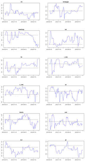
Figure 2.
Expected values of regression coefficients from the EV-TVP-GT model (i.e., equal-weighted averaging of time-varying parameter regressions with the Google Trends index for the search query variable). RPPI denotes the logarithmic differences of Residential Property Price Index, mortgage—logarithmic differences of the level of mortgages in thousands of TRY, dwellings—the number of two or more dwelling residential buildings, cpi—logarithmic differences of Consumer Price Index, fdi—foreign direct investment in real estate activities, i_rate—interest rate for housing, ipi—Industrial Production Index, u_rate—unemployment rate, stocks—logarithmic differences of Borsa Istanbul 100 Index, usd—logarithmic differences of the USD/TRY exchange rate, eur—logarithmic differences of the EUR/TRY exchange rate, gt—the Google Trends index for the search query, ird—the difference between the 10-year Turkish bond yield and 2-year bond yield. All variables were additionally standardized.
The results of the analysis show that the effects of dwellings, i_rate, stocks, and usd quotation variables on RPPI differ. The mentioned variables often affect RPPI in a mixed way that is not clear and generally follows a fluctuating course. After the 2008 crisis, the Turkish government and the Central Bank of Turkey implemented many policies (especially those aimed at housing loans) to stimulate supply and demand in the real estate market. Consequently, those policies caused many macro and micro data to give unbalanced and unstable reactions.
Another reason for the unbalanced reactions can be cited as the increasing number of Internet users day by day. The research carried out by Internet users on housing prices literally increases the competition. Accordingly, increasing competition is thought to cause more price fluctuations. Based on this, the effect of the gt (Google Trends index) variable included in the model on the RPPI (housing price index) was found negative. As a result, this finding can be interpreted in two different ways. Firstly, the research carried out by millions of Internet users on housing increases competition among firms that supply housing. Increased competition leads to price cuts among housing firms, and this may allow consumers to buy houses at lower prices. Secondly, this counterintuitive occurrence can be in line with the findings that the Internet search queries do not improve the forecast accuracy of RPPI within the considered modeling framework.
Another result can be interpreted from the analysis that government bond yields (ird) around 2012 had a positive impact on RPPI and in 2016 had a negative impact. According to the theory, during periods when interest rates rise, investors often invest their savings either by buying government bonds or by investing in banks to generate interest income. Therefore, investments do not turn into either commercial or residential investments. In Turkey, this scenario took place after 2008, with interest rates declining in 2011 and then, around 2012, yields on government bonds declining also. Accordingly, the shift of investors' interest and investment in the housing market rather than government bonds was reflected in the analysis results. Moreover, this situation may also cause an increase in housing prices.
Another finding of the analysis was in relation to mortgage lending. Notably, the mortgage loans used have a positive effect on RPPI at regular intervals. It is thought that credit standards, loan conditions, down payment amounts, and mortgage amounts differ or change over time, preventing the reflection of mortgage loans on the RPPI from continuing stably. Loan options that allow payment with long-term mortgage loans in housing purchases positively affect the amount of housing demand. According to the analysis results, the mortgage system, which came into force in 2006 but was affected by the 2008 crisis, had a positive impact on house prices in Turkey after 2010.
A further novel finding is that the effect of inflation on RPPI is often positive, except for some short-term characteristics. As expected economically, a similar direction occurred between inflation and housing prices. The positive relationship between inflation and house prices is thought to be related to Turkey's inflationary environment. According to this environment, housing is seen as a mechanism of protection against inflation and a safe investment tool. Therefore, a positive relationship between inflation and house prices in Turkey is not surprising.
The positive effect of FDI on RPPI has been seen since the impact of the crisis decreased. This period coincides with the year 2014. This is thought to have the effect of facilitating the acquisition of real estate in Turkey by non-Turkish citizens coming from abroad through legal arrangements.
The results cast a light on the findings of u_rate and ipi variables of the study. The u_rate effect was positive, while the ipi effect was often negative. This result provides evidence that these two variables act together. When industrial production drops, unemployment will increase and household income will decrease. Consequently, this slowdown in the economy will also negatively affect the construction sector. This economic slowdown, which has caused housing stocks to decline eventually, has triggered an increase in housing prices.
The findings pointed to a similar expected result, with the euro effect on RPPI often being negative. In particular, Turkey’s export revenues, which trade in the European Union, are generally realized in euros. In fact, realized euro valuations against Turkish liras (TL) cause less income and loss of wealth. As a result, the demand for housing for consumers suffering from income and wealth is decreasing. The results of the analysis confirm this relationship and show the negative relationship of the euro with RPPI.
6. Conclusions, Limitations, and Recommendations
Especially after the global financial crisis of 2008, the importance of the housing market for the macro economies of countries increased the academic interest in housing markets. As exemplified by this study, Turkey’s unique economic and sociocultural structural changes (such as migration from the countryside to the city, urban renewal projects, and mortgage lending) have further increased this importance. Accordingly, determining the factors affecting housing prices can be useful in guiding the strategies of both the house seekers and investors. Moreover, identifying the key driving forces behind real estate prices could help market authorities to safeguard stability in real estate markets and prevent the creation of future bubbles therein.
In this study, unlike previous experimental studies, the factors affecting house prices were composed by adding the Google Trends index variable and by using the DMA technique, which has different advantages and has not been used in Turkey before. Dynamic model averaging (DMA) is gaining increasing attention in macroeconomic time series forecasting due to its ability to accommodate time variation in both the parameters as well as the specification of the optimal predicting model. Moreover, various statistical methods have been applied by comparing the prediction performance of DMA with that of other benchmark models. Additionally, this analysis uses the Google Trends index as a supplementary predictor beyond the traditional economic variables to predict changes.
In this study, the analyzed period covers the time period between January 2010 and December 2019 in Turkey. According to the results, ird, mortgage, fdi, u_rate, ipi, eur, and gt variables were used to predict the price of housing in Turkey. Therefore, this study gives an idea about which macro data can be estimated with housing prices in Turkey. However, the same situation is not the case for dwellings, i_rate, stocks, and usd variables. According to analysis results, it can be seen that around 2012 the impact of ird was positive on RPPI, whereas around 2016 it was negative. The impact of mortgage was positive around 2011, 2014, and in recent periods. The impact of dwellings has been negative recently, whereas around 2015 it was mostly positive. The impact of cpi is positive most of the time, except for some short-term peculiarities. Similarly, the impact of fdi has been positive since 2014, but before it was quite often negative. The impact of i_rate is highly time-varying. Recently, it has been negative. It is also interesting that for many periods the impact of u_rate was positive. The impact of ipi was negative most of the time. The impact of stocks was positive around 2016, but recently it has been negative, similar to 2011 and 2012. The impact of the EUR exchange rate was negative most of the time, but the relationship with the USD exchange rate is more volatile. Finally, the impact of the gt variable is negative most of the time.
It is necessary to underscore several important issues as the limitations of the research. First, data constraints blocked the way for this research to be conducted more broadly. For example, variables such as GDP and household income, which may have an impact on housing prices, could not be included in the model due to their limited publication frequency. Moreover, many factors, such as credit conditions and standards, the variability of down payment amounts, and differing mortgage rates, are among the limitations of the research. Another limitation is the Google Trends index variable used. The Google Trends index variable is not a variable that can be directly controlled and presented by the government like any other received variable. To increase the eligibility and quality of the housing price statistics, the presentation of such an index by the government will increase the reliability of the work to be done in this regard.
In conclusion, this research shows that the housing market has an important role in transferring macroeconomic variables and macro policy decisions to the real economy. Moreover, the analysis in this article can be expanded by making various country comparisons. Thus, not only can house prices be analyzed, but the interaction with benchmarking in different countries can also be examined. In addition to the countries, it is necessary to emphasize the need for city officers to monitor house prices. Determining the impact of housing affordability and housing price on the economic and social development of a city will inform policymakers about important development indicators and, in return, help them develop sustainable appropriate strategies. The most important suggestion to be given as a result of this study is that researchers, consumers, and, most importantly, policymakers should use housing prices as a leading indicator and should constantly monitor the housing market.
Author Contributions
Conceptualization, N.H., K.D. and I.H.E.; Data curation, K.D. and I.H.E.; Formal analysis, N.H., K.D. and I.H.E.; Funding acquisition, K.D.; Investigation, N.H., K.D. and I.H.E.; Methodology, K.D.; Project administration, I.H.E.; Resources, I.H.E.; Software, K.D.; Supervision, I.H.E.; Validation, K.D.; Visualization, N.H., K.D. and I.H.E.; Writing—original draft, N.H., K.D. and I.H.E.; Writing—review & editing, N.H., K.D. and I.H.E.. All authors have read and agreed to the published version of the manuscript.
Funding
This research received no external funding.
Data Availability Statement
Data are available upon a request. Data collection and pre-processing is described in details in the paper allowing for replication of the results. Data are publicly provided by the original sources cited in the paper. Due to the copyright issues the collected data are not published in a separate form publicly.
Conflicts of Interest
The authors declare no conflict of interest.
Appendix A
Table A1.
The MCS test.
Table A1.
The MCS test.
| SE | ASE | |
|---|---|---|
| DMA | −0.6579 | −1.0477 |
| DMS | 0.1261 | 0.3598 |
| MPM | 1.3425 | 1.1648 |
| BMA | −0.0381 | 0.4697 |
| BMS | 0.4229 | 0.8635 |
| BMPM | −0.1054 | −0.1416 |
| EV-TVP | −1.4743 | −2.2625 |
| TVP | 0.4537 | 0.9888 |
| LASSO | 0.0398 | 0.6405 |
| ARIMA | −0.9485 | −1.7138 |
| DMA-GT | −1.1835 | −2.4125 |
| DMS-GT | 0.5049 | 0.0296 |
| MPM-GT | 0.3762 | −0.2659 |
| BMA-GT | −0.2509 | 0.2031 |
| BMS-GT | 0.5187 | 0.3719 |
| BMPM-GT | 0.0739 | −0.9252 |
| EV-TVP-GT | −3.3681 | −5.0890 |
| TVP-GT | −0.3203 | 0.3534 |
| LASSO-GT | −0.4915 | 0.0192 |
| ARIMA-GT | −2.1890 | −2.2108 |
| NAÏVE | 1.1984 | 1.9412 |
Notes: The table reports the “Tmax” statistics. The model names are explained in the text. SE denotes squared error loss function, ASE—absolute scaled error loss function. DMA denotes dynamic model averaging, DMS—dynamic model selection, MPM—median probability model, BMA—Bayesian model averaging, BMS—Bayesian model selection, BMPM—Bayesian median probability model, EV-TVP—equal-weighted averaging of time-varying parameter regressions, TVP—time-varying parameter regression, LASSO—lasso penalized regression, ARIMA—autoregressive integrated moving average model, NAÏVE—the naïve forecast, i.e., no-change one. “-GT” indicates that the model includes the Google Trends index for the search query.

Figure A1.
Real observed values and forecasts from DMA-GT and EV-TVP-GT models. The model names are explained in the text. DMA denotes dynamic model averaging, EV-TVP—equal-weighted averaging of time-varying parameter regressions. “-GT” indicates that the model includes the Google Trends index for the search query.
Note
| 1 | AREREIT (2019a) reported in Turkey and in the world construction sector consistent acceleration and profitability that occur in the real estate sector. |
References
- Adams, Zeno, and Roland Füss. 2010. Macroeconomic determinants of international housing markets. Journal of Housing Economics 19: 38–50. [Google Scholar] [CrossRef]
- Afşar, Asli, Özgur Yılmazel, and Sibel Yılmazel. 2017. Konut fiyatlarini etkileyen faktörlerin hedonik model ile belirlenmesi: Eskişehir Örneği. Selçuk Üniversitesi Sosyal Bilimler Enstitüsü Dergisi 37: 195–205. [Google Scholar]
- Akinsomi, Omolokolade, Aye Godness, C. Babalos Vassilios, Fotini Economou, and Rangan Gupta. 2016. Real estate returns predictability revisited: Novel evidence from the US REITs market. Empirical Economics 51: 1165–90. [Google Scholar] [CrossRef]
- Aizenman, Jashua, and Yothin Jinjarak. 2014. Real estate valuation, current account and credit growth patterns, before and after the 2008–9 crisis. Journal of International Money and Finance 48: 249–70. [Google Scholar] [CrossRef][Green Version]
- Akkaş, Murat Engin, and Güven Sayılgan. 2015. Fiyatlari ve konut kredisi faizi: Toda-Yamamoto nedensellik testi. Journal of Economics, Finance and Accounting 2: 572–83. [Google Scholar]
- Al-Masum, Md Abdullah, and Lin Chyi Lee. 2019. Modelling housing prices and market fundamentals: Evidence from the Sydney housing market. International Journal of Housing Markets and Analysis 12: 746–62. [Google Scholar] [CrossRef]
- Alp, Esra. 2019. Macroeconomic Determinants of Rental House Prices In Turkey. Bankacılar Dergisi 30: 94–113. [Google Scholar]
- Anundsen, Andre K., Karsten Gerdrup, Frank Hansen, and Kasper Kragh-Sørensen. 2016. Bubbles and crises: The role of house prices and credit. Journal of Applied Econometrics 31: 1291–311. [Google Scholar] [CrossRef]
- AREREIT. 2019a. Restate Turkey: A Close Look to Comparable Markets. The Association of Real Estate and Real Estate Investment Companies Report, Issue: 2. İstanbul: AREREIT. [Google Scholar]
- AREREIT. 2019b. Gyoder Gösterge: Türkiye Gayrimenkul Sektörü 2019 3. Çeyrek Raporu. The Association of Real Estate and Real Estate Investment Companies Report, Sayı: 18. İstanbul: AREREIT. [Google Scholar]
- AREREIT. 2019c. Türkiye’de A’dan Z’ye Mülk Edinme Rehberi. The Association of Real Estate and Real Estate Investment Companies Report. İstanbul: AREREIT. [Google Scholar]
- AREREIT. 2020a. Restate Turkey: A Close Look to Comparable Markets. The Association of Real Estate and Real Estate Investment Companies Report, Issue: 3. İstanbul: AREREIT. [Google Scholar]
- AREREIT. 2020b. Gösterge: Türkiye Gayrımenkul Sektörü 2020. The Association of Real Estate and Real Estate Investment Companies Report, Sayı: 20. İstanbul: AREREIT. [Google Scholar]
- Arsenault, Marcel, Jim Clayton, and Liang Peng. 2013. Mortgage fund flows, capital appreciation, and real estate cycles. The Journal of Real Estate Finance and Economics 47: 243–65. [Google Scholar] [CrossRef]
- Arslan, Gözde, and Hicran Kasa. 2020. The Importance of Land, Housing, and Property Prices in Asset Prices Channel. Third Sector Social Economic Review 55: 758–71. [Google Scholar]
- Aye, Goodness, Rangan Gupta, Shawkat Hammoudeh, and Woon Joong Kim. 2015. Forecasting the price of gold using dynamic model averaging. International Review of Financial Analysis 41: 257–66. [Google Scholar] [CrossRef]
- Barbieri, Maria, and James Berger. 2004. Optimal predictive model selection. The Annals of Statistics 32: 870–97. [Google Scholar] [CrossRef]
- Baur, Dirk, Joscha Beckmann, and Robert Czudaj. 2016. A melting pot—Gold price forecasts under model and parameter uncertainty. International Review of Financial Analysis 48: 282–91. [Google Scholar] [CrossRef]
- Beltratti, Andrea, and Claudio Morana. 2010. International house prices and macroeconomic fluctuations. Journal of Banking & Finance 34: 533–45. [Google Scholar]
- Beracha, Eli, and Babajide M. Wintoki. 2013. Forecasting residential real estate price changes from online search activity. Journal of Real Estate Research 35: 283–312. [Google Scholar] [CrossRef]
- Bernardi, Mauro, and Leopoldo Catania. 2018. The model confidence set package for R. International Journal of Computational Economics 8: 144–58. [Google Scholar] [CrossRef]
- Berry, Mike, and Tony Dalton. 2004. Housing prices and policy dilemmas: A peculiarly Australian problem? Urban Policy and Research 22: 69–91. [Google Scholar] [CrossRef]
- Bilik, Mustafa, and Üzeyir Aydin. 2019. Konut sahibi olma kararlarını etkileyen faktörler: Lojistik regresyon ve destek vektör makinelerinin karşılaştırılması. Dumlupınar Üniversitesi Sosyal Bilimler Dergisi 62: 184–99. [Google Scholar]
- Bin, Okmyung. 2004. A prediction comparison of housing sales prices by parametric versus semi-parametric regressions. Journal of Housing Economics 13: 68–84. [Google Scholar] [CrossRef]
- Bork, Lasse, and Stig V. Moller. 2015. Forecasting house prices in the 50 states using dynamic model averaging and dynamic model selection. International Journal of Forecasting 31: 63–78. [Google Scholar] [CrossRef]
- Case, Karl E., John M. Quigley, and Rober J. Shiller. 2005. Comparing wealth effects: The stock market versus the housing market. Advances in Macroeconomics 5: 1–32. [Google Scholar] [CrossRef]
- Choi, Huyunyoung, and Hal Varian. 2012. Predicting the present with Google Trends. Economic Record 88: 2–9. [Google Scholar] [CrossRef]
- Chow, Hwee Kwan, and Taojun Xie. 2016. Are House Prices Driven by Capital Flows? Evidence from Singapore. Journal of International Commerce, Economics and Policy 7: 1–21. [Google Scholar] [CrossRef]
- Coskun, Yener. 2016. Property Prices and Investment: An Analysis for Turkey. Nigde Universitesi Iktisadi ve Idari Bilimler Fakultesi Dergisi 9: 201–17. [Google Scholar]
- Dalkılıç, Bahadır, and Mustafa Aşkın. 2018. Gayrimenkul ve konut sektörüne bakış. Emlak Konut: GYO. [Google Scholar]
- Das, Prashant, Alan Ziobrowski, and Edward N. Coulson. 2015. Online information search, market fundamentals and apartment real estate. The Journal of Real Estate Finance and Economics 51: 480–502. [Google Scholar] [CrossRef][Green Version]
- Daşkiran, Filiz. 2015. Denizli Kentinde Konut Talebine Etki Eden Faktörlerin Hedonik Fiyatlandirma Modeli İle Tahmin Edilmesi. Journal of International Social Research 8: 850–57. [Google Scholar] [CrossRef]
- Diebold, Francis X., and Roberto S. Mariano. 1995. Comparing predictive accuracy. Journal of Business and Economic Statistics 13: 253–63. [Google Scholar]
- Drachal, Krzysztof. 2018. multDM: Multivariate Version of the Diebold-Mariano Test. Available online: https://CRAN.R-project.org/package=multDM (accessed on 22 March 2020).
- Drachal, Krzysztof. 2019a. Determining time-varying drivers of spot oil price in a Dynamic Model Averaging framework. Energies 11: 1207. [Google Scholar] [CrossRef]
- Drachal, Krzysztof. 2019b. Dynamic Model Averaging in economics and finance with fDMA: A package for R. Signals 1: 4. [Google Scholar] [CrossRef]
- Ford, James Scott, Ronald C. Rutherford, and Abdullah Yavas. 2005. The effects of the internet on marketing residential real estate. Journal of Housing Economics 14: 92–108. [Google Scholar] [CrossRef]
- Fotheringham, A. Steward, Ricardo Crespo, and Jing Yao. 2015. Exploring, modelling and predicting spatiotemporal variations in house prices. The Annals of Regional Science 54: 417–36. [Google Scholar] [CrossRef]
- Franses, Philip Hans. 2016. A note on the Mean Absolute Scaled Error. International Journal of Forecasting 32: 20–22. [Google Scholar] [CrossRef]
- Friedman, Benjamin M., and Kenneth N. Kuttner. 1993. Economic Activity and The Short Term Credit Markets: An Analysis of Prices and Quantities. Brookings Paper on Economic Activities 2: 193–285. [Google Scholar] [CrossRef]
- Friedman, Jerome, Trevor Hastie, and Rob Tibshirani. 2010. Regularization paths for generalized linear models via coordinate descent. Journal of Statistical Software 33: 1–22. [Google Scholar] [CrossRef] [PubMed]
- Fry, Renee A., Vance L. Martin, and Nicholas Voukelatos. 2010. Overvaluation in Australian housing and equity markets: Wealth effects or monetary policy? The Economic Record 86: 465–85. [Google Scholar] [CrossRef]
- Gebeşoğlu, Pinar Fulya. 2019. Housing Price Index Dynamics in Turkey. Journal of Yaşar University 14: 100–7. [Google Scholar]
- Ghysels, Eric, Alberto Plazzi, Roseen Valkanov, and Walter Torous. 2013. Forecasting real estate prices. In Handbook of Economic Forecasting. Edited by Graham Elliott and Allan Timmermann. Amsterdam: Elsevier, pp. 509–80. [Google Scholar]
- Ginsberg, Jeremy, Matthew H. Mohebbi, Rajan S. Patel, Lynnette Brammer, Mark S. Smolinski, and Larry Brilliant. 2009. Detecting influenza epidemics using search engine query data. Nature 457: 1012–14. [Google Scholar] [CrossRef]
- Glaeser, Edward L., and Charles G. Nathanson. 2017. An extrapolative model of house price dynamics. Journal of Financial Economics 126: 147–70. [Google Scholar] [CrossRef]
- Google. 2020. Available online: https://trends.google.com/trends (accessed on 22 March 2020).
- Guest, Ross, and Nicholas Rohde. 2017. The contribution of foreign real estate investment to housing price growth in Australian capital cities. Abacus 53: 304–18. [Google Scholar] [CrossRef]
- Gupta, Rangan, Alain Kabundi, and Stephan M. Miller. 2011. Using large data sets to forecast house prices: A case study of twenty U.S. states. Journal of Housing Research 20: 161–90. [Google Scholar] [CrossRef]
- Güler, İsmet, Uğur Başer, and Mehmet Bozoğlu. 2019. Rize İli Merkez İlçesinde Konut Fiyatlarının Hedonik Fiyat Modeliyle Değerlemesi. Iğdır Üniversitesi Fen Bilimleri Enstitüsü Dergisi 9: 2294–302. [Google Scholar]
- Hadavandi, Esmaeil, Arash Ghanbari, S. Mohsen Mirjani, and Salman Abbasian. 2011. An econometric panel data-based approach for housing price forecasting in Iran. International Journal of Housing Markets and Analysis 4: 70–83. [Google Scholar] [CrossRef]
- Hansen, Peter R., Asger Lunde, and James M. Nason. 2011. The model confidence set. Econometrica 79: 453–97. [Google Scholar] [CrossRef]
- Harrison, David, Jr., and Daniel L. Rubinfeld. 1978. Hedonic housing prices and the demand for clean air. Journal of Environmental Economics and Management 5: 81–102. [Google Scholar] [CrossRef]
- Hohenstatt, Ralf, Manuel Käsbauer, and Wolfgang Schäfers. 2011. “Geco” and its potential for real estate research: Evidence from the US housing market. Journal of Real Estate Research 33: 471–506. [Google Scholar] [CrossRef]
- Hongyu, Liu, Yun W. Park, and Zheng Siqi. 2002. The Interaction Between Housing Investment and Economic Growth in China. International Real Estate Review 5: 40–60. [Google Scholar]
- Hyndman, Rob J., and Anne B. Koehler. 2006. Another look at measures of forecast accuracy. International Journal of Forecasting 22: 679–88. [Google Scholar] [CrossRef]
- Hyndman, Rob, and Yeasmin Khandakar. 2008. Automatic time series forecasting: The forecast package for R. Journal of Statistical Software 26: 1–22. [Google Scholar]
- İslamoğlu, Bahar, and Şaban Nazlıoğlu. 2019. Enflasyon ve Konut Fiyatları: Istanbul, Ankara ve Izmir için panel veri analizi. Siyaset, Ekonomi ve Yönetim Araştırmaları Dergisi 7: 93–99. [Google Scholar]
- JLL. 2020. The Real Estate Sector in Turkey Report, Republic of Turkey Prime Minister Investment Support. Available online: https://www.invest.gov.tr/en/library/publications/lists/investpublications/real-estate-industry.pdf (accessed on 5 June 2021).
- Karadaş, Hüseyin Ali, and Esengül Salihoglu. 2020. The Effect of Selected Macroeconomıc Varıables on Housıng Prıces: The Case of Turkey. The International Journal of Economic and Social Research 16: 63–80. [Google Scholar]
- Karny, Miroslav, ed. 2006. Optimized Bayesian Dynamic Advising. Berlin: Springer. [Google Scholar]
- Kishor, Kundan N., and Hardik A. Marfatia. 2018. Forecasting house prices in OECD economies. Journal of Forecasting 37: 170–90. [Google Scholar] [CrossRef]
- Kolcu, Fatma, and Nebiye Yamak. 2018. Gelir ve Faiz Oranlarının Konut Fiyatları Üzerindeki Kısa ve Uzun Dönem Etkileri. Uluslararası İktisadi ve İdari İncelemeler Dergisi, 141–52. [Google Scholar] [CrossRef]
- Koop, Garry, and Dimitris Korobilis. 2011. UK macroeconomic forecasting with many predictors: Which models forecast best and when do they do so? Economic Modelling 28: 2307–18. [Google Scholar] [CrossRef]
- Koop, Garry, and Dimitris Korobilis. 2013. Large time-varying parameter VARs. Journal of Econometrics 177: 185–98. [Google Scholar] [CrossRef]
- Kördiş, Gizem, Sayım Işık, and Mehmet Mert. 2014. Antalya’da Konut Fiyatlarını Etkileyen Faktörlerin Hedonik Fiyat Modeli ile Tahmin Edilmesi. Akdeniz İ.İ.B.F. Dergisi 28: 103–32. [Google Scholar]
- Kulkarni, Rajenda, Kingsley E. Haynes, Roger R. Stough, and Jean H. Paelinck. 2009. Forecasting housing prices with Google econometrics. GMU School of Public Policy Research Paper 10: 1–37. [Google Scholar] [CrossRef]
- Lancaster, Kelvin J. 1966a. A new approach to consumer theory. Journal of Political Economy 74: 132–57. [Google Scholar] [CrossRef]
- Lancaster, Kelvin J. 1966b. Change and innovation in the technology of consumption. The American Economic Review 56: 14–23. [Google Scholar]
- Li, Mingche M., and H. James Brown. 1980. Micro-neighborhood externalities and hedonic housing prices. Land Economics 56: 125–41. [Google Scholar] [CrossRef]
- Li, Sheng, Yi Jiang, Shuisong Ke, Ke Nie, and Chao Wu. 2021. Understanding the Effects of Influential Factors on Housing Prices by Combining Extreme Gradient Boosting and a Hedonic Price Model (XGBoost-HPM). Land 10: 533. [Google Scholar] [CrossRef]
- Liu, Tian, Wejyan Hu, Yang Song, and Anlu Zhang. 2020. Exploring spillover effects of ecological lands: A spatial multilevel hedonic price model of the housing market in Wuhan, China. Ecological Economics 170: 1–9. [Google Scholar] [CrossRef]
- Liu, Xiaolong. 2013. Spatial and temporal dependence in house price prediction. The Journal of Real Estate Finance and Economics 47: 341–69. [Google Scholar] [CrossRef]
- Luo, Zhenqiang, Chunlu Liu, and David Picken. 2007. Granger causality among house price and macro-economic variables in Victoria. Pacific Rim Property Research Journal 13: 234–56. [Google Scholar] [CrossRef]
- Mariano, Roberto S., and Daniel Preve. 2012. Statistical tests for multiple forecast comparison. Journal of Econometrics 169: 123–30. [Google Scholar] [CrossRef]
- Milcheva, Stanimira, and Steffen Sebastian. 2010. Housing channels of monetary policy transmission in European industrial and transition countries. European Real Estate Society 159: 1–67. [Google Scholar]
- Mishkin, Frederic S. 2001. The Transmission Mechanism and the Role of Asset Prices in Monetary Policy. NBER Working Paper 8617. Cambridge: National Bureau of Economic Research. [Google Scholar]
- Nicholls, Sarah. 2019. Impacts of environmental disturbances on housing prices: A review of the hedonic pricing literature. Journal of Environmental Management 246: 1–10. [Google Scholar] [CrossRef]
- Nuuter, Tiina, Irene Lill, and Laura Tupenaite. 2014. Ranking of housing market sustainability in selected European Countries. WSEAS Transactions on Business and Economics 11: 778–86. [Google Scholar]
- Paul, Pascal. 2018. Historical Patterns of Inequality and Productivity around Financial Crises. Federal Reserve Bank of San Francisco Working Paper 2017-23. San Francisco: Federal Reserve Bank of San Francisco. [Google Scholar]
- Paul, Pascal. 2019. The Time-Varying Effect of Monetary Policy on Asset Prices. Federal Reserve Bank of San Francisco Working Paper 2017-09. San Francisco: Federal Reserve Bank of San Francisco. [Google Scholar] [CrossRef]
- R Core Team. 2018. R: A Language and Environment for Statistical Computing. Vienna: R Foundation for Statistical Computing. Available online: https://www.R-project.org (accessed on 22 March 2020).
- Raftery, Adrian, Miroslav Karny, and Pavel Ettler. 2010. Online prediction under model uncertainty via dynamic model averaging: Application to a cold rolling mill. Technometrics 52: 52–66. [Google Scholar] [CrossRef]
- Risse, Marian, and Martin Kern. 2016. Forecasting house-price growth in the Euro area with dynamic model averaging. The North American Journal of Economics and Finance 38: 70–85. [Google Scholar] [CrossRef]
- Rosen, Sherwin. 1974. Hedonic prices and implicit markets: Product differentiation in pure competition. Journal of Political Economy 82: 34–55. [Google Scholar] [CrossRef]
- Sağlam, Can, and Zehra Abdioğlu. 2020. Türkiye’de Tüketici Fiyatları ile Hedonik Konut Fiyatları Arasındaki İlişki: Panel Veri Analizi. Journal of Yasar University 15: 117–28. [Google Scholar]
- Sari, Ramazan, Bradley T. Ewing, and Bahar Aydin. 2007. Macroeconomic variables and the housing market in Turkey. Emerging Markets Finance and Trade 43: 5–19. [Google Scholar] [CrossRef]
- Shi, Song, Vince Mangioni, Xin Janet Ge, Shanaka Herath, Fethi Rabhi, and Rachida Ouysse. 2021. House Price Forecasting from Investment Perspectives. Land 10: 1009. [Google Scholar] [CrossRef]
- Shimshoni, Yair, Niv Efron, and Yossi Matias. 2009. On the Predictability of Search Trends. Israel Labs: Google. [Google Scholar]
- Sirmans, Stacy, David Macpherson, and Emily Zietz. 2005. The composition of hedonic pricing models. Journal of Real Estate Literature 13: 1–44. [Google Scholar] [CrossRef]
- Sousa, Diogo. 2018. Forecasting House Prices Using Dynamic Model Averaging. Ph.D. dissertation, Finance from the NOVA—School of Business and Economics, Lisbon, Portugal. [Google Scholar]
- Stadelmann, David. 2010. Which factors capitalize into house prices? A Bayesian averaging approach. Journal of Housing Economics 19: 180–204. [Google Scholar] [CrossRef]
- Stevenson, Simon, and James Young. 2014. A multiple error-correction model of housing supply. Housing Studies 29: 362–79. [Google Scholar] [CrossRef]
- Stooq. 2020. Available online: https://stooq.com (accessed on 22 March 2020).
- Su, Chi-Wei Su, Xiao-Qing Wang, Ran Tao, and Hsu-Ling Chang. 2019. Does money supply drive housing prices in China? International Review of Economics and Finance 60: 85–94. [Google Scholar] [CrossRef]
- Tibshirani, Robert. 1996. Regression shrinkage and selection via the lasso. Journal of the Royal Statistical Society. Series B 58: 267–88. [Google Scholar] [CrossRef]
- Turkish Central Bank. 2020. Available online: https://www.tcmb.gov.tr (accessed on 22 March 2020).
- Uyar, Kangallı, Sinem Güler, and Nihal Yayla. 2016. Konut Fiyatlarının Hedonik Fiyatlama Yaklaşımına Göre Mekânsal Ekonometrik Modeller ile Tahmini: İstanbul Konut Piyasası Örneği. Social Sciences (NWSASOS) 3C0153 11: 326–42. [Google Scholar]
- Wang, Zhimin, Jung Hoon, and Benson Lim. 2012. The impacts of housing affordability on social and economic sustainability in Beijing. Australasian Journal of Construction Economics and Building-Conference Series 1: 47–55. [Google Scholar] [CrossRef]
- Wei, Yu, and Yang Cao. 2017. Forecasting house prices using dynamic model averaging approach: Evidence from China. Economic Modelling 61: 147–55. [Google Scholar] [CrossRef]
- Wu, Lynn, and Eric Brynjolfsson. 2015. The future of prediction: How Google searches foreshadow housing prices and sales. In Economic Analysis of the Digital Economy. Chicago: University of Chicago Press. [Google Scholar]
- Yayar, Rüştü, and Deniz Gül. 2014. Mersin Kent Merkezinde Konut Piyasası Fiyatlarının Hedonik Tahmini. Anadolu Üniversitesi Sosyal Bilimler Dergisi 14: 87–100. [Google Scholar]
- Yemelina, Natalya, Ainura Omarova, and Anara Kurmanalina. 2018. Analysis and forecast of prices of the housing market. Journal of Applied Economic Sciences 13: 843–51. [Google Scholar]
- Yıldırım, Mustafa Ozan. 2017. Türkiye Ekonomisinde Konut Piyasası Dinamiklerinin Analizi. Ph.D. dissertation, Pamukkale Üniversitesi Sosyal Bilimler Enstitüsü, Denizli, Turkey. [Google Scholar]
- Yılmazel, Özgür, Aslı Afşar, and Sibel Yılmazel. 2018. Konut Fiyat Tahmininde Yapay Sinir Ağları Yönteminin Kullanılması. International Journal of Economic and Administrative Studies 20: 285–300. [Google Scholar] [CrossRef]
- Yusupova, Alisa, Nicos G. Pavlidis, and Efthymios G. Pavlidis. 2019. Adaptive Dynamic Model Averaging with an Application to House Price Forecasting. arXiv arXiv:1912.04661. [Google Scholar]
- Zhang, Yanbing, Xiuping Hua, and Liang Zhao. 2012. Exploring determinants of housing prices: A case study of Chinese experience in 1999–2010. Economic Modelling 29: 2349–61. [Google Scholar] [CrossRef]
Publisher’s Note: MDPI stays neutral with regard to jurisdictional claims in published maps and institutional affiliations. |
© 2022 by the authors. Licensee MDPI, Basel, Switzerland. This article is an open access article distributed under the terms and conditions of the Creative Commons Attribution (CC BY) license (https://creativecommons.org/licenses/by/4.0/).