1. Introduction
On 11 March 2020, the World Health Organization officially declared the coronavirus (COVID-19) outbreak to be a global pandemic. In more than a few months the COVID-19 pandemic spreaded across the world, paralyzing daily economic and social life. While the numbers of affected individuals are increasing and the global economic impacts are unclear, the financial markets are no exception either. During the year 2020, many countries recorded a drop in the stock exchange indexes. Some of the countries, such as the USA, recorded the highest plunge in the stock index in the 21st century, whereas countries such as New Zealand did not experience such a decrease. According to
Shehzad et al. (
2020), the USA and Europe financial markets were more affected by the COVID-19 pandemic compared to Asian financial markets; moreover, Asian financial markets provide greater opportunities to diversify financial risks.
Most of the studies on the impact of the COVID-19 pandemic on stock markets are based either on the analysis of a relatively short period (the beginning or the “first wave” of the pandemic) or a longer period, which, in turn, is very heterogeneous in terms of both the information available on the COVID-19 virus and the measures taken to contain the virus and address the consequences of the pandemic. However, it is very important to assess the impact not only at the beginning of the pandemic but also in the subsequent periods and to compare the nature of this impact; the studies of this type are still fragmentary. Therefore, this paper aims to investigate the impact of the COVID-19 pandemic on the stock exchange indexes in Italy and Spain during the period of 1 March 2020 to 30 November 2020, dividing it into three phases of different characteristics.
The selection of these countries for the research is based on the fact that both countries had tremendous financial and economic consequences regarding the virus pandemic. Experiencing the disclosure of the financial markets led to a significant drop in share prices; therefore, in response to such events, the Italian FTSE MIB 40 and Spanish IBEX 35 stock indexes decreased as well. The selection of two individual countries instead of a wider sample is based on the need to analyze the response of individual stock markets instead of accumulated global or regional response since the response of the countries in the sample may be of the opposite nature. For example,
Cheong et al. (
2020) analyzed if the financial markets overreacted to the COVID-19 pandemic from December 2019 to January 2020 and February 2020 to March 2020. According to the provided descriptive statistics, many selected sample countries’ financial markets reacted to COVID-19 spread during the first period, except Malaysia and Thailand. Yet, during the February to March 2020 period, all countries had a lower negative mean of returns. The MSCI World Index recorded highs that were higher than the first pandemic period in Australia, Singapore, Thailand, and the United States of America.
Thus, as is stated by
Cheong et al. (
2020): (i) every country has different effects from the pandemic, and it is important to understand that such a phenomenon cannot be studied in a generalized way; and (ii) the global or regional samples will not provide correct conclusions—instead, the focus should be pointed to individual countries and their macro- and micro-level reactions to the COVID-19 pandemic.
Unlike other studies, this research aims to investigate the impact of COVID-19 on Italy (FTSE MIB 40) and Spain (IBEX 35) stock exchange indexes during the three separate periods: period 1—1 March to 31 May 2020; period 2—1 June to 31 August 2020; period 3—1 September to 30 November 2020, covering two waves of pandemic and the recovery period between them. These periods at least partially coincide with the first wave of the pandemic, the so-called quiet period, and the second wave of the pandemic. This allows us not only to evaluate the impact of the COVID-19 pandemic on stock markets quantitatively but also to compare this impact during the different periods or the phases of the pandemic, at the same time perceiving critical and stabilization periods. On the one hand, as is stated by
Ciner (
2021), stabilization of the stock markets is crucial to seeking economic recovery in the face of the COVID-19 pandemic and after it; on the other hand, it is very important to learn the lesson from such a rare pandemic, because there is a possibility that mankind will encounter similar “unusual disasters” in the future. It is the analysis of the effect of the COVID-19 pandemic on stock markets that provides a unique opportunity to identify the patterns for future preparations.
The number of confirmed cases of COVID-19 infection is selected as an independent variable, the FTSE MIB 40 and IBEX 35 indexes are selected as dependent variables, and the CBOE Volatility Index is selected as a control variable for our research. To reach the aim of this study, and based on previous studies, the research of three stages is conducted employing the following methods: (i) simple OLS (bivariate) regression, the ARCH-LM test, and robust Heteroskedasticity and Autocorrelation Consistent Covariance Method (HAC); (ii) VAR-based impulse response functions; (iii) GARCH (1,1) model; the average and percentage changes of index values and their volatility (measured as standard deviation) are also analyzed to confirm the results of regression analysis.
The most important contribution of this research to the existing literature is that even if the impact of the COVID-19 pandemic on financial markets has been widely analyzed recently, the analysis of separate stages of the pandemic is not still widely developed. Thus, this research provides a comprehensive impact assessment both during the whole pre-vaccination period of the pandemic and during different stages of this period.
The rest of this paper is structured as follows: (i) in
Section 2, the main findings of the analysis of academic literature in the field of the COVID-19 impact on stock markets are discussed; (ii) in
Section 3, the assumptions and design of the research are described; (iii) in
Section 4, the results of the assessment of the impact of the COVID-19 pandemic on stock markets are discussed and compared; and, finally, (iv) the conclusions, limitations, and directions for future research are presented.
2. Literature Review
As well as other financial markets, the stock markets have been inevitably affected by the COVID-19 pandemic—uncertainty in the financial world increased, expectations of market participants deteriorated. The primary negative shock was sudden and severe, in some respects even compared to the Great Financial Crisis of the year 2007–2008.On 12 March 2020, it was stated that “It was a historic day on Wall Street. The Dow plunged 10% for its worst day since Black Monday in 1987. The 30-stock index fell 2352 points—its largest point drop on record. Meanwhile, the S&P 500 plunged 9% to close in the bear market territory, thus officially ending the bull market that began in 2009 during the throes of the financial crisis” (
Stevens et al. 2020). A couple of days later, S&P Global reported that “It’s now clear that the hit to global economic activity from the measures to slow the spread of the coronavirus pandemic will be massive” (
S&P Global Report 2020).
For example,
Ben Haddad et al. (
2021) have analyzed the volatility in commodity markets and found out that the COVID-19-pandemic-induced crisis has caused one of the highest volatility periods from the 1960s.
Rakha et al. (
2021) employed artificial intelligence and data from previous crises to assess and predict the economic impact of the COVID-19 pandemic in the United Kingdom; predictions showed a steady growth of GDP in 2021, although at around −8.5% contraction in comparison with pre-pandemic forecasts.
Sansa (
2020) investigated if there was an impact of the COVID-19 on the financial markets in the USA within the period of 1 March 2020 to 25 March 2020. The research results revealed a positive relationship between the COVID-19 confirmed cases and New York Dow Jones Financial Stock. The research of
Yousaf et al. (
2020) revealed the increased volatility of stock market return in Russia, India, Brazil, and Peru.
Ashraf (
2020) researched proof that stock markets react to new COVID-19 cases, but not the fatalities. According to panel pooled ordinary least squares regression results, the increase in confirmed cases variable is negative and more significant, in comparison with the growth in the deaths variable, and it loses significance when daily fixed-effects dummy variables are added into the model. Thus, the author confirms that daily growth in COVID-19 confirmed cases has a strong negative correlation with stock market returns in 64 selected sample countries. However, the growth in the deaths variable also has a negative result, yet the stock market response to the number of deaths is relatively low. Findings suggest that stock market prices react strongly during the early days of confirmed cases and less when confirmed cases die later on.
O’Donnell et al. (
2021) also examined the responses of China, Italy, Spain, the UK and the USA equity indexes to the growth of COVID-19 confirmed cases and confirmed that the equity index faced a significant negative shock due to the increasing number of COVID-19 confirmed cases. Analyzing the sample of the top 10 countries,
Zhang et al. (
2020) also revealed that the growth of confirmed cases is related to the increase in risk levels; the important role of market sentiment is highlighted.
Czech et al. (
2020) analyzed the COVID-19 impact on the financial markets of Visegrad Group countries and used the TGARCH model to measure the impact of COVID-19 cases on the exchange rates and stock market volatility. The results revealed that the COVID-19 pandemic had a negative impact on the Visegrad financial markets and that during the pandemic the volatility increased (
Czech et al. 2020).
Ramelli and Wagner (
2020) analyzed how international companies reacted in the first months of the COVID-19 pandemic outburst. Researchers selected to investigate three periods from the beginning of January to the end of March 2020. The results provided information that the COVID-19 pandemic issue topic accrued more often on calls in companies that have a stronger connection with international trade and also companies that have higher liquidity risks. The approach of selecting the different periods provided results with concerns that varied from period to period. For example, the international trade concern was mostly discussed during the outbreak period, while the liquidity topic was discussed in the fever (last) period. Thus, the financial state and international trade concerns in the companies were discussed in different periods and concluded that such factors had an important effect on stock market reactions.
Ibrahim et al. (
2020) analyzed the relationship between the COVID-19 pandemic in its first wave, response measures implemented by governments, and stock market volatility in Asia-Pacific countries. The results indicated increased levels of volatility in the face of pandemic and stabilizing effects of government measures.
Ftiti et al. (
2021) revealed that the COVID-19 crisis negatively affected the Shanghai stock market—price volatility increased and the level of liquidity decreased. According to the researchers, the knock-on effect was caused by an unprepared healthcare system, when the crisis-induced supply shock directly harmed the financial market.
Izzeldin et al. (
2021) used the most recent data available from G7 countries’ (USA, UK, France, Japan, Germany, Italy, and Canada) stock markets and categorized volatility analysis in 10 business sectors. The findings of this research revealed that: (i) the sectors of health care and consumer services were the most severely affected by the COVID-19 pandemic, (ii) while the sectors of telecommunications and technology were affected the least severely; (iii) United Kingdom and United States of America financial markets were affected the most, yet with big response heterogeneity across the business sectors.
Dias et al. (
2020) have also analyzed G7 countries and revealed that during the period from 31 December 2019 to 23 July 2020, most markets displayed structure breaks between February and March 2020, because of global pandemic disruption. Furthermore, the findings of
Wang and Enilov (
2020) suggest that COVID-19 was able to establish a dominant short-term influence on the stock movement in financial markets, and it appears that it has the most significant effect on the largest advanced economies in the world.
The COVID-19 pandemic appeared to have a stronger effect on American and European stock markets compared to Asian stock markets. Despite the fact that in February 2020 China’s markets demonstrated a high level of uncertainty (measured by standard deviation), it decreased substantially in March 2020. At the same time, the US market volatility (measured by standard deviation) in March 2020 appeared to be nearly four times higher than in February 2020 (
Zhang et al. 2020). Consumer spending in the Euro Area decreased from EUR 1532.09 billion to EUR 1463.141 billion in the first quarter of 2020 (Eurostat Database). Furthermore, after most of the Eurozone countries imposed strict quarantine and citizens were isolated in their houses, consumer spending decreased to EUR 1282.21 billion in the second quarter of 2020. In addition, the Eurozone economy’s gross domestic product shrank by 11.8% in the second quarter, whereas in the second quarter of 2019 it was increasing by 0.1% (
Trading Economics 2020). Nevertheless, in the third quarter of 2020 “The Eurozone economy grew by 12.6 percent in the three months to September 2020, recovering from a record slump of 11.8 percent in the previous period and compared with early estimates of a 12.7 percent advance. It was the steepest pace of expansion since 1995” (
Trading Economics 2020). These unprecedented circumstances led to the growth of scientific studies (for example,
Frezza et al. 2020;
Klose and Tillmann 2021;
Bonaccolto et al. 2019;
Nieto and Rubio 2020;
Ahmar and del Val 2020; and others) concentrating on European stock markets and their reaction to the spread of the COVID-19 pandemic.
Using the multifractional Brownian motion as a model of the price dynamics,
Frezza et al. (
2020) analyzed the influence of the COVID-19 pandemic on the efficiency of 15 European financial markets; the pattern before and after the two pandemic crashes was estimated; the results revealed that European markets’ recovery of efficiency lasted not for long and, in accordance with the model, the volatility is still too high to be compatible with market efficiency.
Bonaccolto et al. (
2019) provided some evidence of an increase in the conversion risk for France and Italy since the beginning of January 2020. According to
Nieto and Rubio (
2020), analysis of the Spanish stock market revealed that, due to the COVID-19 pandemic, IBEX 35 stock index decreased significantly, and volatility increased to levels similar to the Great Recession (
Nieto and Rubio 2020). Thus, rising uncertainty worldwide and an increase in risk aversion formed the behavior of financial markets during the first two quarters of the year 2020. Nevertheless,
Ahmar and del Val (
2020) determined that the Spanish stock market began to stabilize on the 24 March 2020.
A number of studies (for example,
Fassas 2020;
Kanapickiene et al. 2020;
Albulescu 2020;
Huynh et al. 2021;
Panyagometh 2020) analyze the impact of the spread of the COVID-19 pandemic on the sentiment of financial market participants as well as on a broad economic sentiment. For example,
Kanapickiene et al. (
2020) analyzed the relationship between pandemic and economic sentiment and determined that customer sentiment was not so volatile as business sentiment. The results of
Albulescu’s (
2020) study demonstrated that VIX, the so-called “fear factor”, showing overall uncertainty in financial markets, significantly increased at the beginning of the COVID-19 pandemic.
Huynh et al. (
2021) analyzed investor sentiment in the face of the COVID-19 pandemic and pointed out that such countries as the United Kingdom, China, the United States, and Germany experienced sentimental shocks; moreover, these shocks were transmitted to other markets. Those shocks were also confirmed by the study conducted by
Panyagometh (
2020), which also indicated a negative reaction of Thailand’s stock market.
Fassas (
2020) analyzed connectedness across the variance risk premium in both developed and emerging equity markets and revealed that, due to the COVIDI-19 pandemic, the interconnectedness of investor sentiment, as well as the degree of risk aversion, increased.
Finally, it is important to mention that the impact of the COVID-19 pandemic on financial markets has led to changes in the efficiency of standard economic policy measures. For example, using the method of panel analysis for European countries,
Klose and Tillmann (
2021) determined that: (i) announcements of policy initiatives and regulation adjustments positively assisted some countries and led to a slight increase in stock prices; (ii) the increasing number of COVID-19 cases raised bond yields, showing deteriorating investor expectations; (iii) announcements of national liquidity assistance programs and national fiscal policy add input in rising the bond yields; (iv) purchase programs of the central bank led to raised stock prices and reduced bond yields; and (v) countries which are affected by increasing the growth of COVID-19 cases could face an increase in bond yields on days of a fiscal policy announcement, whereas the same announcement in less affected countries keeps yields unchanged.
Wei and Han (
2021), using the sample of 37 severely affected countries, estimated the impact on the transmission of monetary policy to financial markets in the face of the COVID-19 pandemic and revealed that, during the 2020 COVID-19 pandemic period, both conventional and unconventional monetary policy had significant effects on the financial markets, including exchange rate, governmental bond, CDS markets, and stocks. However, unconventional monetary policies were more effective, rather than conventional policies, since they can affect the stock, exchange rate, and markets to some degree.
Further, the design of our research is discussed.
3. Research Methodology
3.1. Data Selection
As mentioned in previous sections, seeking to achieve the main purpose of this research, i.e., to assess the impact of the COVID-19 pandemic on the European stock markets, the stock markets of Italy and Spain are selected for further research.
As is stated by
Borri (
2020), Italy is assumed to be one of the first European economies struck by the COVID-19 pandemic, as well as one of the most severely affected. Health crisis, the strict lock-down, and unsuspected virus spread for 4 months led to economic and financial problems. Equity markets dropped, first, by roughly 35% in Italy and the rest of the Eurozone; interventions of the central banks at least partially helped to limit uncertainty in financial markets; however, while the United States stock markets regained their potential almost fully later in 2020, the Eurozone and specifically Italy’s market remained about 15% lower than at the beginning of 2020 (
Borri 2020).
Henriquez et al. (
2020) noted that the Spanish stock market was also significantly hit by the COVID-19 pandemic: a significant decrease in the IBEX 35 stock index has been recorded since January 2020. However, in mid-June 2020, a significant increase appeared due to the credit loans for the tourism sector, which played an important role in Spain’s economy (
Instituto Nacional de Estadistica 2020).
As mentioned in the introductory section, unlike previous studies, this research aims to evaluate the impact of the COVID-19 pandemic on Italy (FTSE MIB 40) and Spain (IBEX 35) stock exchange indexes during the two waves of pandemic and the recovery period between them (see
Figure 1a,b). The first period is dated from 1 March 2020 to 31 May 2020, and is selected to represent the beginning or so-called first wave of the spread of the COVID-19 pandemic: from the beginning of March 2020, active cases of COVID-19 started rapidly rising in Italy and Spain, whereas at the end of May it stabilized to numbers similar to those seen at the beginning of March; thus, according to researchers, it was cited as the first wave of the COVID-19 pandemic. The second period is dated from 1 June 2020 to 31 August 2020, and is selected to represent the so-called quiet period after the beginning of the first wave of a pandemic: during the summer of 2020, both Italy and Spain had a stable and controlled situation without any drastic fluctuations in active cases of COVID-19; therefore, this period was established as a recovery period. Finally, the third period is dated from 1 September 2020 to 30 November 2020, and is selected to represent the second wave of the spread of the COVID-19 pandemic: during this period, the new confirmed cases of COVID-19 raised to new records in both countries, leading people to believe that the second pandemic wave was defined. After the summer 2020 season, both The Ministry of Health in Spain and The Ministry of Health in Italy (
Sen 2020) governmental entities released public statements that one way or another the second wave of the COVID-19 pandemic would take place in the upcoming autumn months. Therefore, Period 3 is analyzed to reveal market reaction during the beginning and middle stages of the second wave of the COVID-19 pandemic. Unlike the research of
Ramelli and Wagner (
2020) (see
Section 2), our research covers longer data series and allows for employing different methods of analysis.
The spread of the COVID-19 pandemic had a tremendous impact on both Italy and Spain during the 1st period (1 March to 31 May 2020): on the one hand, Italy’s financial and health sectors were unprepared for such disaster; on the other hand, the uncontrolled spread of the COVID-19 virus in Spain began later on. That being the case, it is very interesting to analyze and compare how Italian and Spanish stock exchange indexes reacted to the pandemic.
Further, the methods used to analyze this reaction are discussed.
3.2. Research Design
Our research itself consists of three main stages, which are further discussed briefly.
In Stage 1, the regression model is employed to investigate the possible effect of the spread of the COVID-19 pandemic on the Italian and Spanish stock markets. Thus, as is done in similar studies in the field (for example,
Albulescu 2020;
Zhang et al. 2020;
Klose and Tillmann 2021;
Sansa 2020;
Kanapickiene et al. 2020;
Ashraf 2020; and others), in our research, the method of simple OLS (bivariate) regression is chosen as it can efficiently examine the relationship between stock indices and COVID-19 confirmed cases. Simple OLS (bivariate) regression models are created for each period and each country.
It is important to mention that different studies use different COVID-19-related variables, for example, the number of affected countries (
Albulescu 2020), the cumulative number of total cases of COVID-19 infection (
Ashraf 2020;
Al-Awadhi et al. 2020;
Zhang et al. 2020;
Czech et al. 2020) and the daily number of cases of COVID-19 infection (
Albulescu 2020;
Zaremba et al. 2020). Following the recent studies, to reach the main aim of the research, we select the number of newly confirmed cases of COVID-19 infection and the growth rate of this number as an independent variable because we aim to assess how markets respond to the changing situation daily.
As dependent variables, two indexes: the FTSE MIB 40 index (Milano Indice di Borsa) representing the Italian stock market and the IBEX 35 index (Índice Bursátil Español) representing the Spanish stock market, were selected. Natural logarithms of indexes are used for further analysis.
The FTSE MIB 40 (Milano Indice di Borsa) was selected because it is the national Italian stock exchange index, which consists of the 40 top traded stock classes. Moreover, it is a volatile index that frequently sees large moves and double-digit annual changes. According to
AvaTrade (
2021), FTSE MIB 40 includes powerful multi-national companies such as ENI Group, STMicroelectronics, and Fiat Chrysler, along with domestic Italian companies. Thus, the index can be used as an estimate of the overall Italian economy. IBEX 35 (Índice Bursátil Español) was chosen as it represents 35 of the largest Spanish companies, such as Repsol (oil/gas), Santander (finance/banking), and others (
AvaTrade 2021). Thus, the IBEX 35 index can be seen as one of the indicators of the overall view of the Spanish stock market condition. For GARCH model indexes (see
Section 4.3), we use the daily return of selected.
Seeking to assess the robustness of the relationship analyzed, the control variable is also included in the specifications of our models. In this research, the CBOE Volatility Index (VIX) was used as a financial benchmark tracking stock market volatility (on the basis of S&P500 Index option prices). This index was chosen as it measures the expected volatility (market expectations) of the U.S. equity market. According to
Moran and Liu (
2020), VIX is usually negatively correlated with price movements of the stock indexes, and, in periods of sharp decline in stock markets, it tends to rise.
Grima et al. (
2021) used the VIX index to assess the effect of daily new cases and deaths caused by COVID-19 on major stock markets, and
Shankar and Dubey (
2021) included VIX as a control variable in the model assessing the impact of the COVID-19 pandemic on the Indian stock market.
Baek et al. (
2020) also included VIX as a regressor in models measuring the impact of COVID-19 related news on US stock market volatility.
Seeking to check the stationarity of selected variables and their suitability for regression models, before constructing regression models, the unit-root test is conducted and the results of the Augmented Dickey–Fuller test (ADF) are evaluated (data are differenced if necessary) (the ADF test was conducted using a constant, lag length selected using the Schwarz information criterion, max lags = 14). After constructing OLS regression models, they are checked for the heteroscedasticity and residuals—the ARCH effect is tested using the ARCH-LM test (lag length q = 1). In the presence of the ARCH effect, the robust Heteroskedasticity and Autocorrelation Consistent Covariance Method (HAC) is employed and heteroscedasticity-corrected models are created.
In Stage 2, we employ impulse response functions to identify and assess the response of selected index values to the spread of the COVID-19 pandemic. As is done in the studies of
Mzoughi et al. (
2020) and
Brueckner and Vespignani (
2020), we use VAR-based impulse response functions. After all variables are checked for stationarity in Stage 1 (Augmented Dickey–Fuller test), VAR models are constructed when it is meaningful. Lag selection in VAR models is made using Aikake, Schwarz, and Hannan–Quinn information criteria. Finally, using previously described COVID-19-related (as an impulse) and stock-market-related (as a response) variables, we construct impulse response and accumulated impulse response functions.
Finally, in Stage 3, taking into account that the HAC method may not fully correct the influence problems induced by the ARCH effect, we have additionally decided to estimate the GARCH model to assess the impact of the COVID-19 pandemic on the volatility of Italian and Spanish stock markets. We apply the generalized autoregressive conditional heteroscedasticity (GARCH) approach as it is in previous studies (
Gherghina et al. 2021;
Chaudhary et al. 2020;
Duttilo et al. 2021;
Endri et al. 2020). It should be noted that the GARCH model is constructed only in the case of the presence of the ARCH effect (after the ARCH-LM test). We employ the GARCH (1,1) model as a standard and most widely used GARCH-type model. At first, we calculate the daily returns of FTSE MIB 40, and IBEX 35 indexes are calculated using the following formula (natural logarithm difference approach) (
Chaudhary et al. 2020):
where:
Ri,t corresponds to the daily return on index
i at time
t;
Pi,t corresponds to the daily closing price of index
i at time
t; and
Pi,t−1 corresponds to the daily closing price of index
i at time
t − 1.
In case the data series demonstrates heteroscedasticity, they are modeled using the GARCH (1,1) model. In line with
Chaudhary et al. (
2020) and taking into account that we use the COVID-19-related variable (number of daily new cases of infection) as an exogenous variable in the GARCH model, our model can be described as follows:
Conditional Mean Equation
Conditional Variance Equation
where:
yt corresponds to the conditional mean;
ht corresponds to the conditional variance;
and
—constant terms; ε
t—error term of the mean equation;
and
—coefficients of the ARCH and GARCH terms.
Moreover, seeking to complement the results of analysis, the average and percentage changes of index values and their volatility (measured as the average of the monthly standard deviation of index return) are calculated for each country and each of the three periods. Daily data are used. The increase in the standard deviation allows for assuming the increase in volatility in the stock market.
The data of daily COVID-19 cases in Italy and Spain are retrieved from the Our World in Data Coronavirus Pandemic (COVID-19) database, and the data of selected stock indexes are retrieved from the Bloomberg database (research variables are summarized in
Table 1). Collected data are organized and analyzed using the quantitative method technique and application of Eviews11 software package.
Table 1.
Research variables and abbreviations.
Table 1.
Research variables and abbreviations.
| Variable |
|---|
| Abbreviation | Full Name | Source |
|---|
| Dependent variables |
| lnFTSEMIB40t | Natural logarithm of Milano Indice di Borsa—Italian stock market index value | Bloomberg database |
| lnIBEX35t | Natural logarithm of Índice Bursátil Español—Spanish stock market index value | Bloomberg database |
| Ret.FTSEMIB40t | Daily return of Milano Indice di Borsa—Italian stock market index | Bloomberg database |
| Ret.IBEX35t | Daily return of Índice Bursátil Español—Spanish stock market index | Bloomberg database |
| Independent variables |
| grNCITt | Growth of the number of new daily confirmed cases of COVID-19 infection in Italy | Our World in Data Coronavirus Pandemic (COVID-19) database |
| grNCSPt | Growth of the number of new daily confirmed cases of COVID-19 infection in Spain | Our World in Data Coronavirus Pandemic (COVID-19) database |
| NCITt | New daily confirmed cases of COVID-19 infection in Italy | Our World in Data Coronavirus Pandemic (COVID-19) database |
| NCSPt | New daily confirmed cases of COVID-19 infection in Spain | Our World in Data Coronavirus Pandemic (COVID-19) database |
| | Control variable | |
| VIXt | CBOE Volatility Index | Bloomberg database |
Further, the main results of our research are presented.
4. Results and Discussion
In this section, the dynamics of Italian and Spanish stock market indexes are analyzed, and the impact of COVID-19 on Italian and Spanish stock markets is evaluated.
4.1. Trends of Italian and Spanish Stock Markets
In the case of Italy, the COVID-19 pandemic had the biggest effects in Europe on countries’ economies and financial markets during the first two quarters of 2020. By the end of December 2020, more than two million (
World Meters 2021) got sick with the virus.
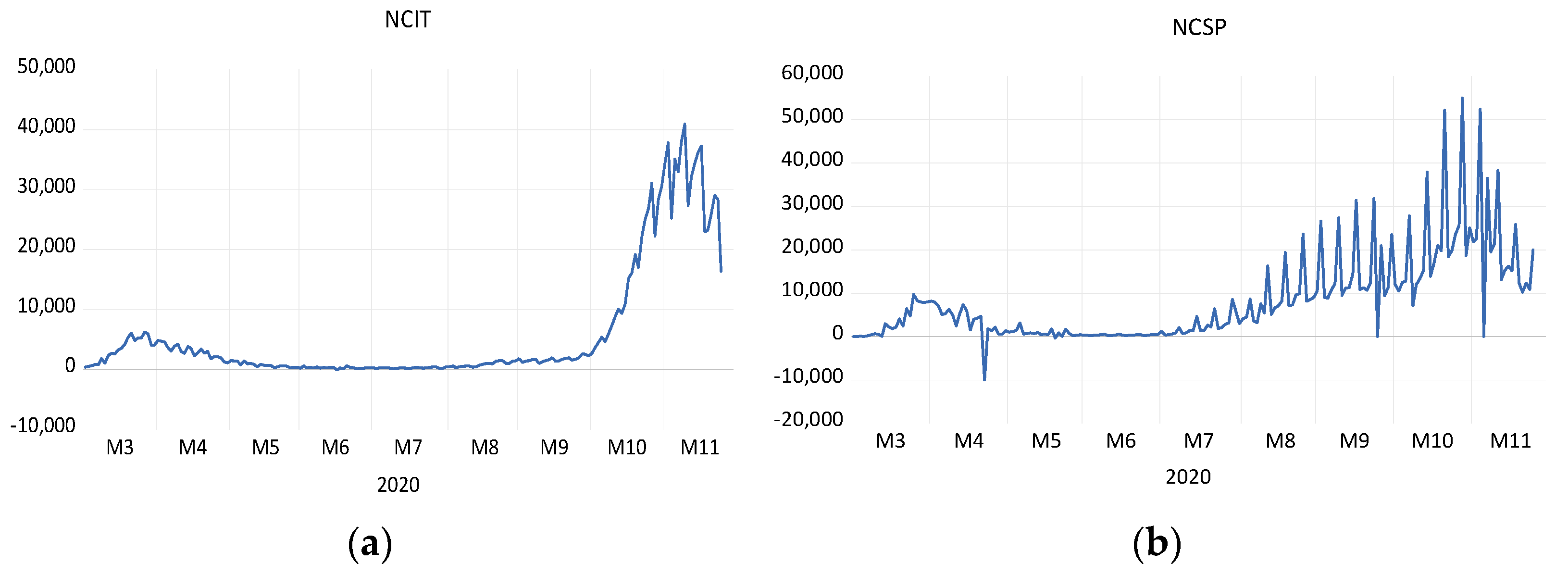
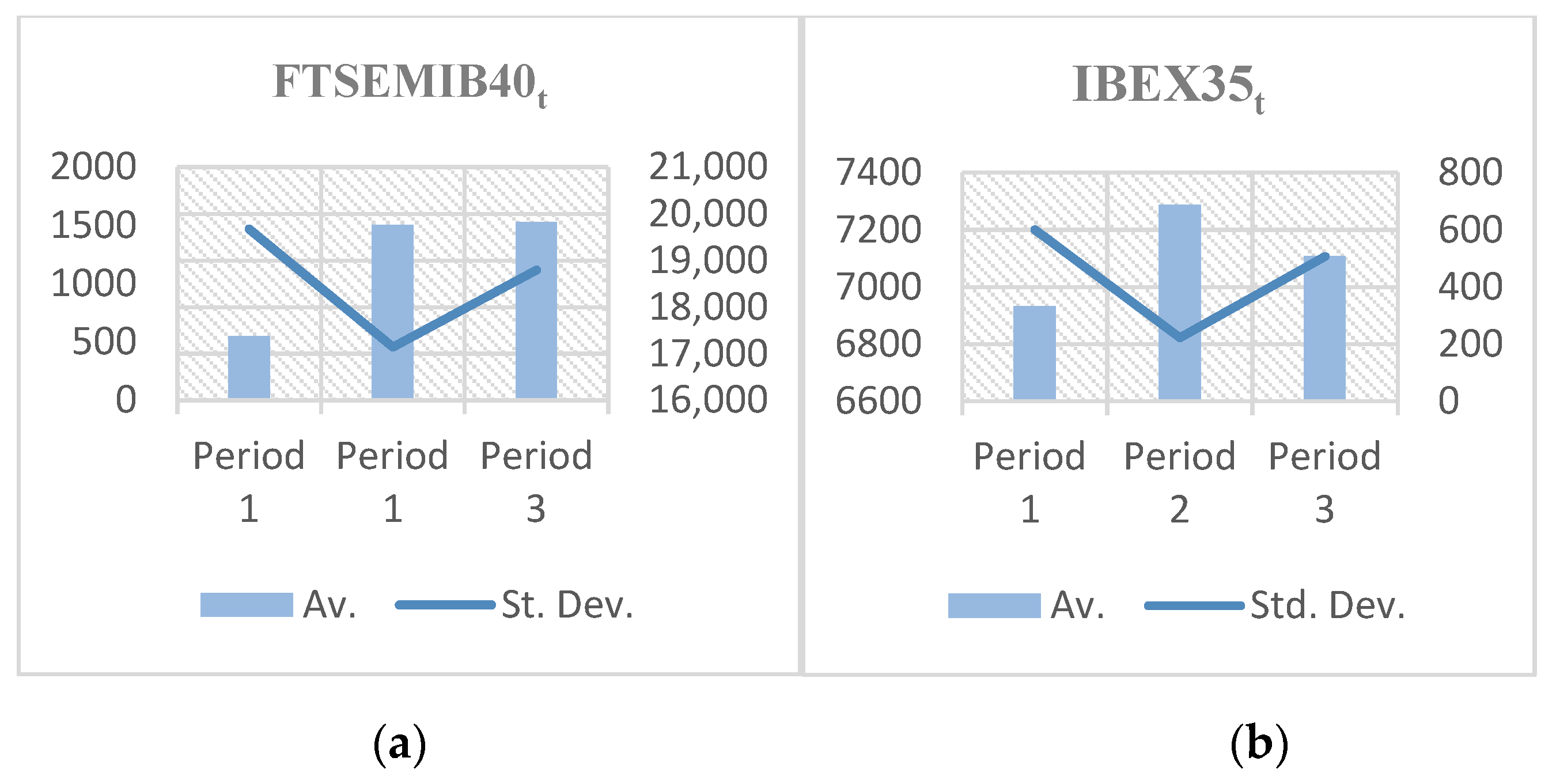
From
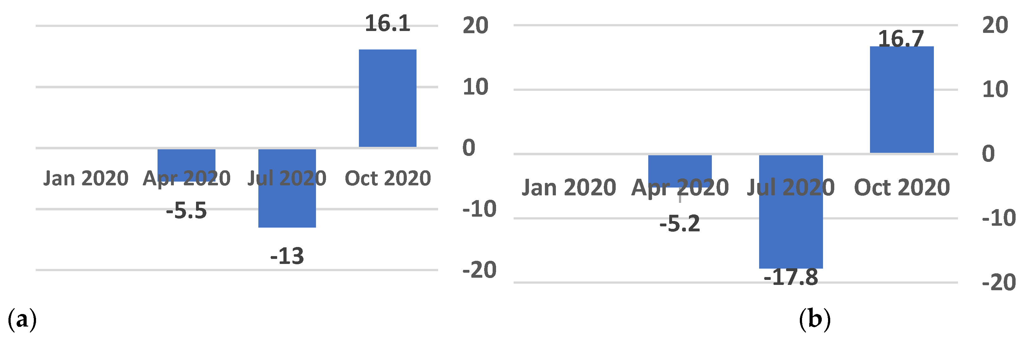
Figure 1a, it is possible to conclude that the pandemic affected the country in two waves: the first wave spread from March 2020 to May 2020; the second one started from October 2020 and it is still ongoing. While the country was in lockdown, which did help to decrease the new cases of infection, the quarantine had severe consequences for economic effect, for example, the gross domestic product (GDP) in Italy shrunk by 13% by the end of the second quarter of 2020, making it was one of the largest drops in the country’s history (see
Figure 2a).
Spain was the second most affected country in Europe by COVID-19 during the first pandemic wave. According to the graph below (see
Figure 1b), there were more than one and a half million confirmed coronavirus cases in Spain up until December 2020. During the first lockdown, the GDP growth rate in Spain shrunk by 17.8%, which is 4.8% more than in Italy. However, in the third quarter, the rate increased by 16.7% (see
Figure 2b), and increasing consumer spending contributed significantly to the GDP.
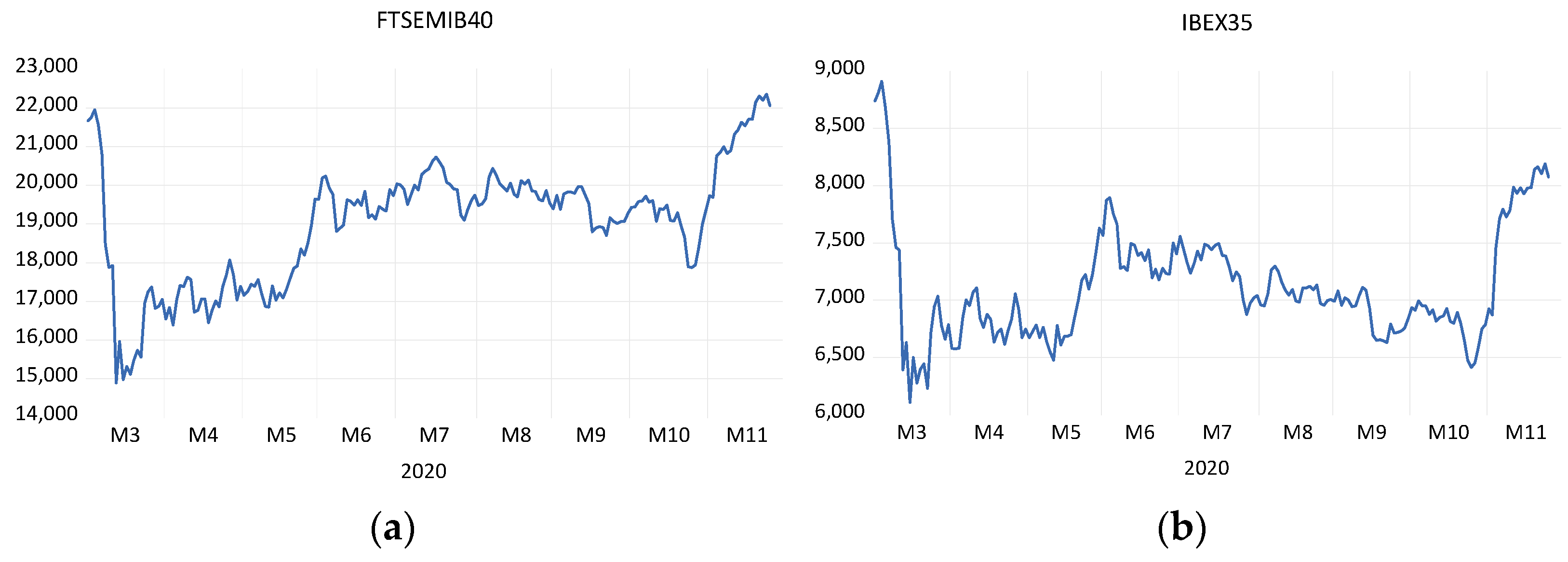
The dynamics of selected Italian and Spanish stock market indexes during the whole period (covering Periods 1–3, 1 March 2020–30 November 2020) are provided in
Figure 3a,b. At the end of the 1st quarter of the year 2020, when the spread of the COVID-19 pandemic was observed in Europe as well, the European stock markets experienced a sudden and strong shock. As it can be seen from
Figure 3, the Italian and Spanish stock markets were no exception either—the significant negative shift in terms of index value can be observed in March 2020. Moreover, FTSE MIB 40 fell by 11% on the 9 March, while IBEX 35 fell by 14% on 12 March; this was recorded as the highest drop in history for one day (
Camarero 2020).
However, after a significant negative shift, observed in the 1st quarter of 2020, Italian and Spanish stock markets regained an upward trend. The second wave of the COVID-19 pandemic was followed by a decrease in index values at the beginning of the 4th quarter of 2020; however, this decline was temporary in nature, and markets adjusted much faster than during the first wave of the pandemic.
Further, the impact of the spread of the COVID-19 pandemic is assessed.
4.2. Assessment of the Impact of the COVID-19 Pandemic on Italian and Spanish Stock Markets
4.2.1. OLS Regression and Heteroscedasticity-Corrected Models
As a starting point, it was attempted to assess the impact of the spread of the COVID-19 pandemic on Italian and Spanish stock markets using simple bivariate (OLS) regression models. Descriptive statistics of OLS regression model variables are provided in
Table 2.
The results of the Augmented Dickey–Fuller test are presented in
Table 3. As can be seen from the table, in the case of selected variables the hypothesis of the presence of a unit root can be rejected, i.e., variables are stationary and can be used in further analysis. Two variables (VIX
t and NCSP
t) appeared to be not stationary in level; thus, in further research, they are used in differences.
Further primary OLS regression models are constructed for each pair of dependent and independent variables and each period (including the whole period). After constructing OLS regression models, they are checked for the heteroscedasticity and residuals using the ARCH-LM test. The results of this test are provided in
Table 4.
As can be seen from
Table 4, the hypothesis of ARCH effect not existing is rejected, i.e., the presence of the ARCH effect is confirmed. Taking this into account, the HAC is employed, and heteroscedasticity-corrected models are created (both primary OLS regression models and heteroscedasticity-corrected models are provided in
Table 5,
Table 6,
Table 7 and
Table 8).
As can be seen from
Table 5, consistent with the results of previous studies (see
Section 2), VIX was confirmed to have a statistically significant negative effect on the values of selected stock indexes. The results in
Table 5 also allow us to state that neither OLS regression models nor heteroscedasticity-corrected models have shown a statistically significant impact of the spread of the COVID-19 pandemic on the values of FTSE MIB 40 and IBEX 35 indexes. Moreover, such analysis does not allow one to assess differences of market response at different stages of the spread of a pandemic, which is why, if one is seeking to examine this effect in greater depth, the analysis of market reactions at separate stages or periods is necessary (the results of which can be seen in
Table 6,
Table 7 and
Table 8).
Interestingly, both OLS regression and heteroscedasticity-corrected models have revealed a positive market reaction to the growth of new daily cases of COVID-19 in the case of Italy in Period 1, even under the control of the selected control variable; the effect of WIX appeared to be negative (
Table 6).
Quite a different situation can be observed in Period 2 (
Table 7) when the effect of the control variable, VIX, turned to be positive, and no statistically significant reaction to the spread of the COVID-19 pandemic can be observed. After the primary shock in Period 1, the uncertainty in the market decreased.
The analysis of the results of both OLS regression models and heteroscedasticity-corrected models for Period 3 does not reveal the statistically significant impact of the COVID-19 pandemic on the Spanish stock market. However, in Period 3 or the onset of the second wave of the pandemic, the growth of new daily reported cases of the infection appeared to have a statistically significant impact on Italy’s stock market (see
Table 8), but only at 90% confidence level. Since the uncertainty in the equity markets increased again, the impact of VIX has proved to be negative on both Italy’s and Spain’s stock markets.
Since the results of this stage do not provide clear evidence of pandemic impact on stock markets, we seek to determine the short-term response of selected indexes representing Italy’s and Spain’s stock markets to the spread of the COVID-19 pandemic using impulse response functions.
4.2.2. VAR-Based Impulse Response Functions
As a starting point, the baseline VAR models, using one dependent and one independent variable mentioned in the previous section, are employed. The results of VAR estimation are provided in
Appendix A,
Appendix C,
Appendix E and
Appendix G, while lag selection criteria can be seen in
Appendix B,
Appendix D,
Appendix F and
Appendix H. Based on these VAR models, the impulse response functions as well as accumulated impulse response functions are created (
Figure 4,
Figure 5,
Figure 6 and
Figure 7). The analysis of these figures allows us to make certain assumptions regarding the direction, strength, and duration of the primary response of FSTE MIB 40 and IBEX 35 indexes in the face of the COVID-19 pandemic.
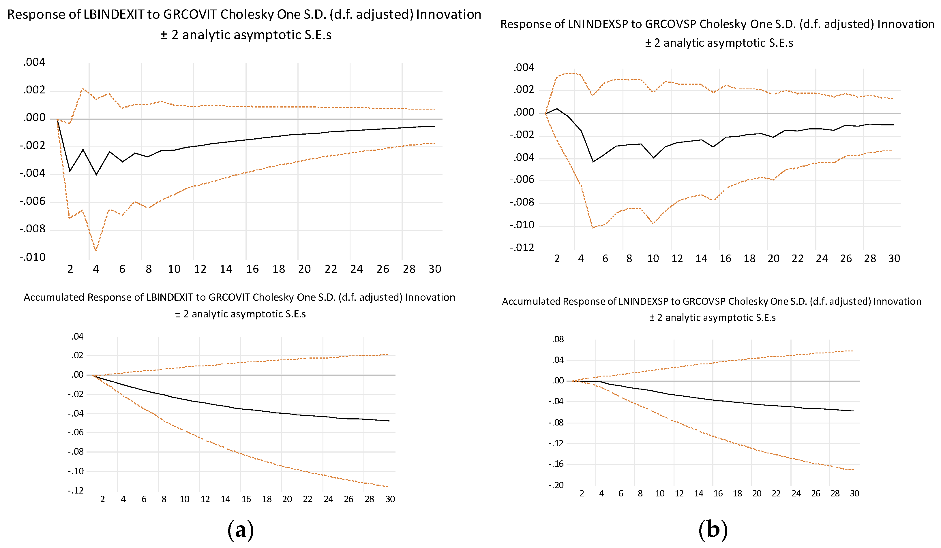
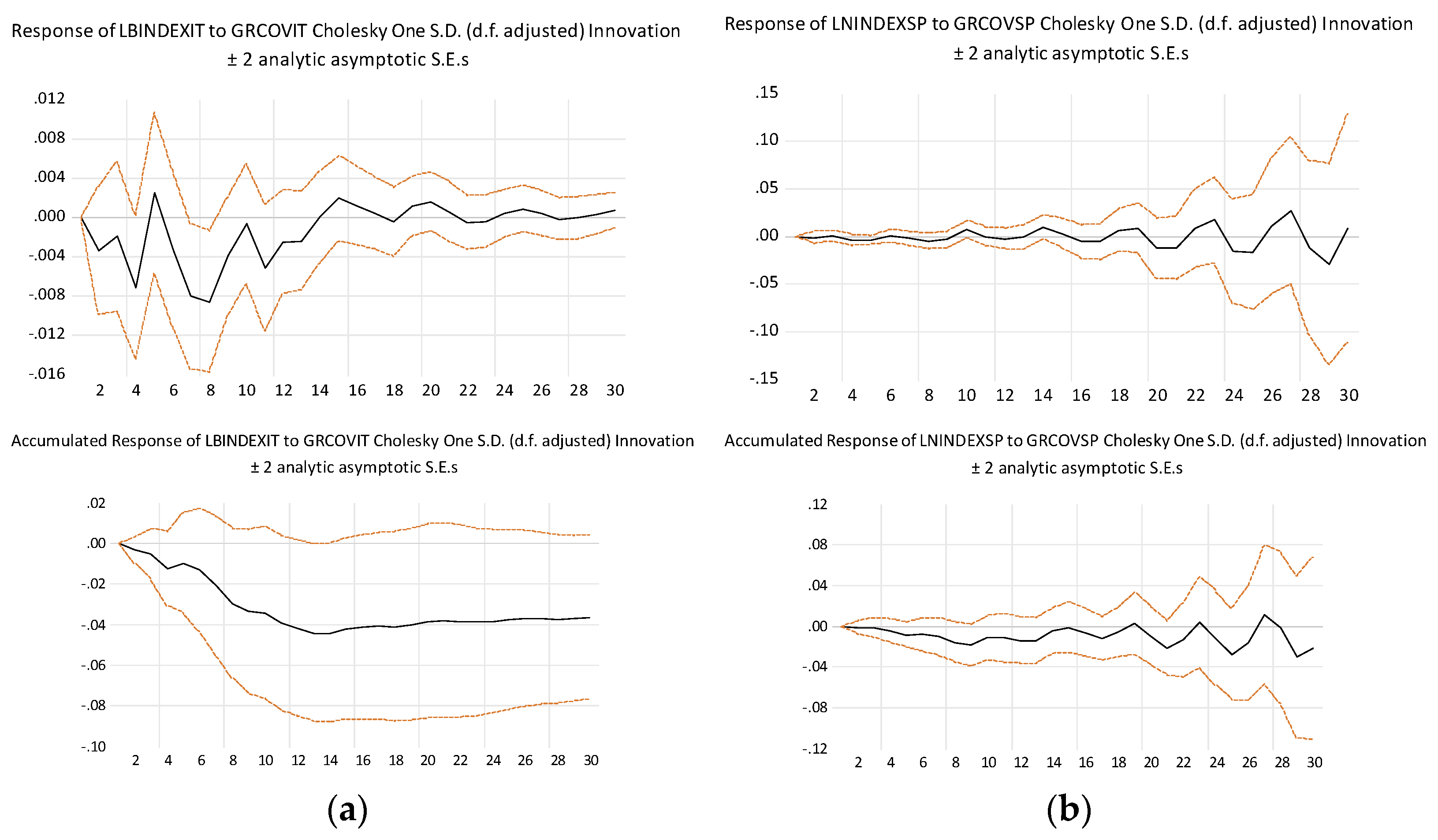
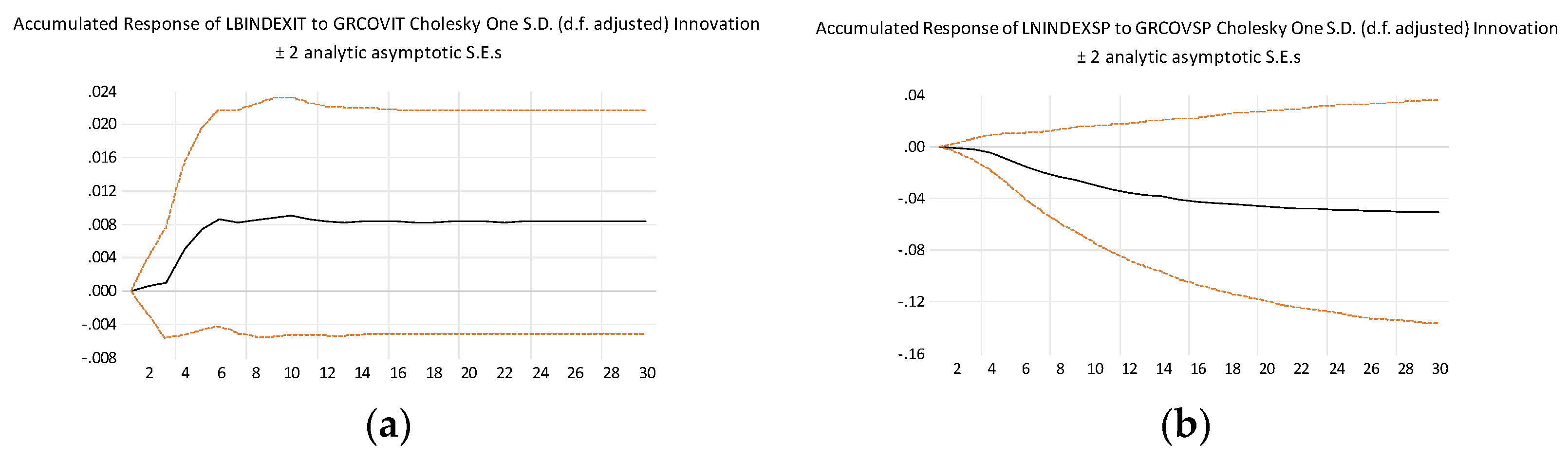
Figure 4 shows the dynamic effects of the growth of COVID-19 cases on the FSTE MIB 40 and IBEX 35 indexes taking into account the whole period. As can be seen, the impulse response functions constructed for the whole period indicate the primary negative response of both FSTE MIB 40 and IBEX 35 indexes in the face of the COVID-19 pandemic. Nevertheless, this response tends to weaken over time and approaches close to zero on day 30. However, the accumulated response appeared to be increasingly negative.
This allows us to assume that the stock markets of Italy and Spain were negatively affected during the early spread of the COVID-19 pandemic. As is stated by World Bank, both Italy and Spain were unprepared for such a massive pandemic; thus, the rapid spread of the COVID-19 pandemic had led to lockdown all across Italy and Spain. According to
Sanfelici (
2020), even though the rapid actions of the government of Italy were taken, the health crisis and lack of planning and communication resulted in policy framework chaos. The first gradual lockdown in Italy was in order on the 23 February, whereas in Spain this was only on the 29 March after the outbreak of the official death toll in Italy, which surpassed that of mainland China (
Davies 2020).
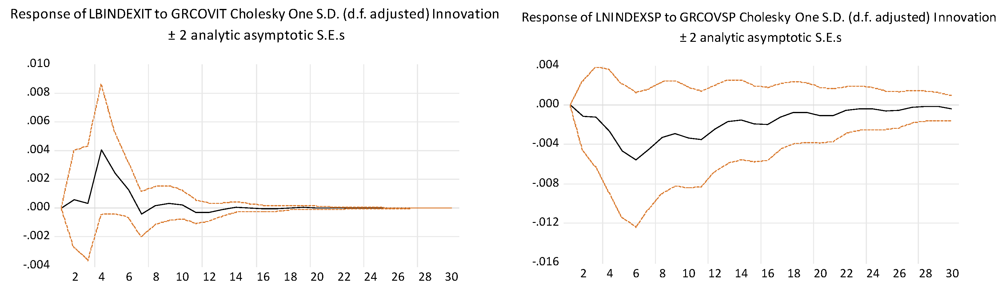
Figure 5 shows the dynamic effects of the growth of COVID-19 cases on the FSTE MIB 40 and IBEX 35 indexes taking into account Period 1, i.e., the first stage of the pandemic.
As can be seen from
Figure 5, the primary response to the COVID-19 pandemic is of inconstant strength and nature; moreover, it slightly differs depending on the country analyzed. In the case of the Italian stock market, the primary response is negative but inconstant, while the accumulated response is negative. In the case of the Spanish stock market, both primary response and accumulated response are close to zero on day 1 and start to fluctuate later on.
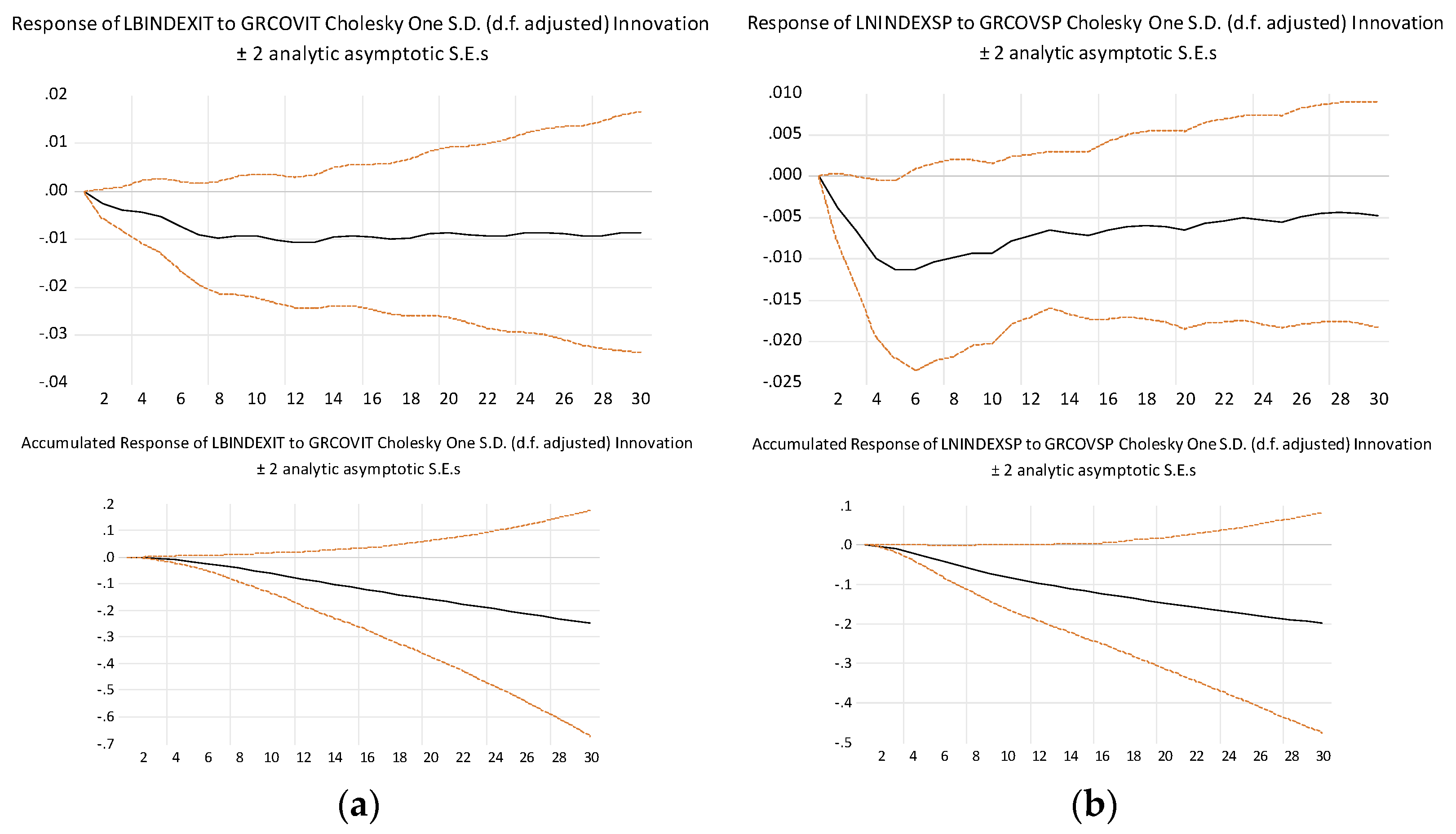
Figure 6 shows the dynamic effects of the growth of COVID-19 cases on the FSTE MIB 40 and IBEX 35 indexes taking into account Period 2, i.e., the recovery period.
As can be seen from
Figure 6, the market reaction during Period 2 differs from the reaction in Period 1 in both Italy and Spain. (i) The initial response of the FTSE MIB 40 index to the spread of the COVID-19 pandemic appeared to be clearly positive, while the initial response of the IBEX 35 index is clearly negative; however, in both cases, the primary response tends to weaken over time and approaches zero in day 20 and 28, respectively. (ii) The accumulated response also differs depending on the country—in the case of Italy, it is positive, while in the case of Spain—negative.
Period 2 can be characterized as the summer season in which the recovery and preparations for the predicted second wave were implied and executed by the governments. During Period 1, Italy had in total 231,869 confirmed cases of COVID-19, while in Period 2 numbers drastically decreased to 36,217 (a decrease of 84.38%). At the same time, the situation in Spain was slightly different: in Period 1, the total number of confirmed cases of COVID-19 was 239,434, and in Period 2 this was 223,379 (a decrease of only 6.71%). Therefore, the results for Period 2 still show a negative impact in the case of Spain.
Different situations in Italy and Spain can be explained by several facts. First of all, during the summer period, Italy’s health system was rebuilt and the COVID-19 testing was quite successful; initially one of the most virus-affected countries, Italy managed to become one of the most successful examples compared to other countries during June, July and August of 2020. Secondly, Italy was one of the first countries that implemented the regional lockdowns around the country; according to Cartabellotta, President of the GIMBE health foundation (
Ians 2021), the mobile hospitals had a major impact on the improvements rather than just using the hospital buildings; moreover, according to the Draghi, the Prime Minister of Italy (
Ians 2021), the country’s vaccine rollout strategy was efficient. Thirdly, Spain faced the COVID-19 pandemic later than Italy; furthermore, the installments of mobile hospitals and virus-controlling strategies also took more time in the later dates in comparison with Italy. Thus, it is possible to conclude that during Period 2, Italy not only reduced its number of confirmed cases of COVID-19 but also demonstrated a sharper recovery of the stock market than Spain. The successful implementation of the government strategies and policies brought effective results, and the research results (
Figure 5 and
Figure 6) also contribute to the evidence.
Figure 7 shows the dynamic effects of the growth of COVID-19 cases on the FSTE MIB 40 and IBEX 35 indexes, taking into account Period 3, i.e., the onset of the second wave of the pandemic.
As is seen from
Figure 7, the impulse response functions constructed for Period 3 indicate both primary and accumulated negative response of both FSTE MIB 40 and IBEX 35 indexes in the face of the COVID-19 pandemic; moreover, this response is of a much more constant nature than in previous periods.
Taking this into account, it can be said that the analysis of VAR-based impulse response functions revealed the non-zero response of selected stock market indexes to the spread of the COVID-19 pandemic. Moreover, this response varies in direction, strength, and duration depending on the country and period analyzed.
4.2.3. GARCH Models
Further, the impact of the COVID-19 pandemic is being analyzed using the GARCH model and using the index return volatility approach.
Figure 8 shows the daily values of FTSE MIB 40 and IBEX 35 index returns calculated using Equation (1). As can be seen from the figure, the returns at the very beginning and the very end of the whole period analyzed are much more volatile than in the rest of the period.
Descriptive statistics of selected dependent (index return) and independent (COVID-19 cases) variables are provided in
Table 9.
The data are further checked for stationarity. The results of the Augmented Dickey–Fuller test are presented in
Table 3. As can be seen from
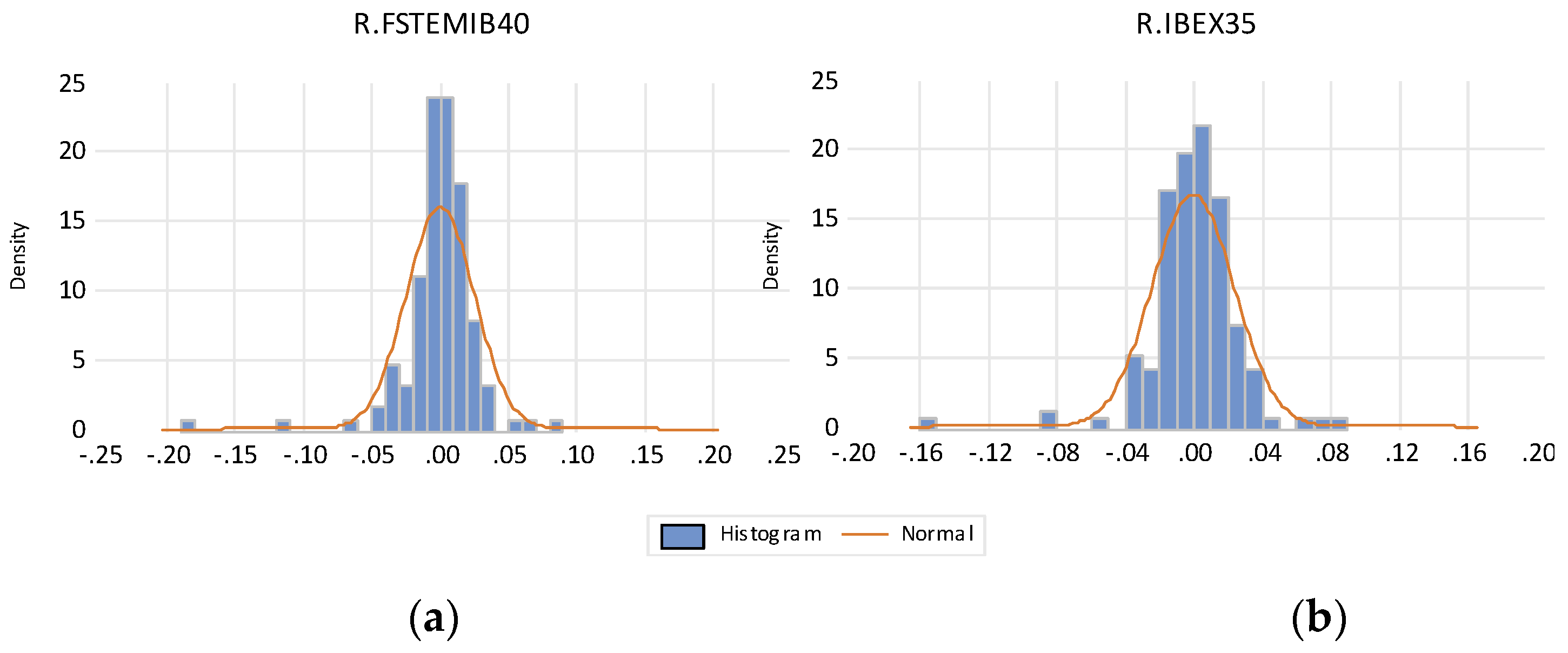
Table 9, the returns of selected indexes are negatively skewed, i.e., demonstrating left-sided asymmetry. The density plots for daily logarithm returns are shown in
Figure 9.
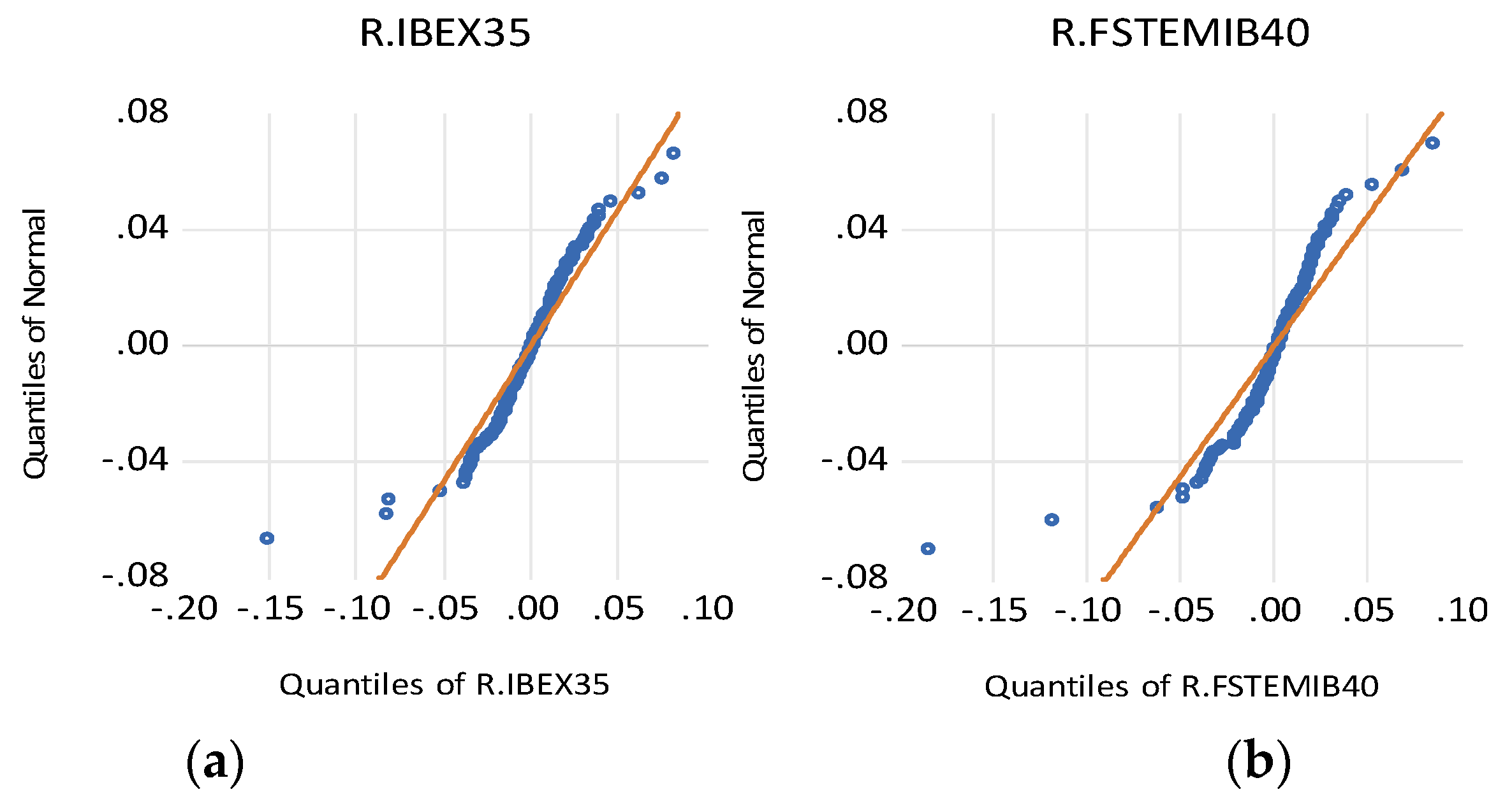
The quantile–quantile plots of logarithm return of selected indexes are shown in
Figure 10. As can be seen from the figure, the distribution of returns of selected indexes differs from the normal (theoretical) distribution.
After checking for the ARCH effect (
Appendix M), we can conclude that, in the case of the return of selected indexes, the ARCH effect is present only in the whole period. As the presence of the ARCH effect can be considered a precondition for the development of the GARCH model, the HAC method is employed and GARCH models are created only for the previously mentioned case, i.e., the whole period, in which the ARCH effect is observed (results of GARCH estimations are provided in
Table 10). For other pairs of variables, only OLS models are analyzed. OLS regression models, as well as heteroscedasticity-corrected models, are provided in
Appendix I,
Appendix J,
Appendix K,
Appendix L. None of these models revealed a statistically significant impact of the spread of the COVID-19 pandemic on the changes of the returns of selected stock market indexes (see
Appendix I,
Appendix J,
Appendix K,
Appendix L). The exception was Period 1 and Period 2 for Italy, where the positive and negative impact (respectively) of the spread of the COVID-19 pandemic was observed. However, models confirmed the negative effect of the control variable—VIX.
The GARCH estimations for FSTEMIB40 and IBEX 35 indexes return in the whole period approach are provided in
Table 10.
The results in
Table 10 reveal a statistically significant GARCH effect and a positive impact of the daily number of COVID-19 cases in the case of the Spanish stock market. A statistically significant GARCH effect is also observed in the case of the Italian stock market. This allows us to state that the spread of the COVID-19 pandemic appeared to have a statistically significant impact on the volatility of the return of stock market indexes analyzed. These results are consistent with those of
Shehzad et al. (
2020) and
Chaudhary et al. (
2020). (Note: it also can be seen from
Table 10 that in the case of the Italian stock market, the GARCH (1,1) is not best suited, as it has negative and statistically insignificant parameters.)
4.3. Discussion of the Results, Limitations, and Directions for Future Research
Figure 11 presents the average volatility measured by the standard variation of Italian and Spanish stock indexes during three analyzed periods.
As can be seen from
Figure 11, from Period 1 to Period 2, the volatility of the FTSE MIB 40 index decreased by more than three times, while the volatility of the IBEX 35 index decreased by more than two times. These results allow us to state the following: (i) after the initial negative shock in Period 1 (the first wave of the COVID-19 pandemic), both the Italian and Spanish stock markets showed significant signs of recovery as the index values rose on average by 13.76% and 5.26%, respectively; (ii) the Italian stock market demonstrated higher growth than the Spanish stock market; (iii) the substantial decrease in volatility in both markets in Period 2 shows that stock markets have adjusted at a certain degree, and the uncertainty, caused inter alia by the rapid spread of the COVID-19 pandemic, decreased substantially; (iv) during the recovery (or so-called quiet period), uncertainty declined more in the Italian than in the Spanish stock market (these results are at least partially confirmed by the results in impulse response function analysis).
Compared to Period 2, in Period 3, volatility increased in both Italian and Spanish stock markets; nevertheless, it appeared to be lower in Period 3 than in Period 1. It is important to note, in comparison with Period 2, that uncertainty in Period 3 increased in both Italian and Spanish markets; nevertheless, during the beginning and middle stages of the second wave of the COVID-19 pandemic (Period 3), both markets were more stable and displayed a lower degree of uncertainty compared to the first wave (Period 1). These results were quite expected because, as mentioned before, during a recovery period (Period 2), there was a favorable time for markets to stabilize and prepare for upcoming higher increases in new COVID-19 cases during the second wave of the pandemic.
The results of this research revealed that the stock market reaction to the spread of the COVID-19 pandemic differs depending on the country and period analyzed. OLS regression and heteroscedasticity-corrected models have not revealed the statistically significant impact of the spread of the COVID-19 pandemic, i.e., the impact appeared to be ambiguous. This mixed (ambiguous) effect of the COVID-19 pandemic was also revealed by
Albulescu (
2020) who analyzed the impact of rising COVID-19 cases and deaths on the volatility of the US stock market.
However, impulse response functions demonstrated the non-zero primary response of analyzed markets to the COVID-19 shock. The primary response during the first and the second wave of the pandemic appeared to be negative in both Italy and Spain. This is consistent with the results obtained by
Ashraf (
2020), who, using VAR-based impulse response functions, revealed that negative market reaction was strong during the early days of COVID-19 cases confirmed. Using the same approach, the negative response of different stock markets was also confirmed by
Ahundjanov et al. (
2020) and
Thakur (
2020). Moreover, the results of impulse response functions revealed that the market reaction was strongest in the first week and weakened later. This is consistent with the results of
Milani (
2021), which revealed that the peak response to the COVID-19 pandemic usually happens 4–6 days after the shock.
Beirne et al. (
2020) also confirmed that the duration of shocks varies in the range of 5 to 10 days.
Interestingly, in the case of Italy, the primary response of the stock market appeared to be positive during the recovery period, which coincides with the results of impulse response functions analysis conducted by
Brueckner and Vespignani (
2020) for the case of Australia.
Finally, GARCH (1;1) models confirmed that the COVID-19 pandemic increased the volatility of stock market return, i.e., the spread of the COVID-19 pandemic appeared to have a statistically significant impact on the volatility of the return of stock market indexes analyzed, which is consistent with the results of
Shehzad et al. (
2020) and
Chaudhary et al. (
2020).
Endri et al. (
2020) also employed GARCH models to prove that stock price volatility increased during the COVID-19 pandemic, which has led to a decrease in returns.
With regard to the contribution of our research, it could be stated that our research covers three separate periods of the COVID-19 pandemic, while a majority of other studies (for example,
Albulescu 2020;
Chaudhary et al. 2020;
Gherghina et al. 2021; and others) analyze data from a much shorter period. We, in turn, develop the analysis of separate stages of the pandemic and provide a comprehensive impact assessment both during the whole pre-vaccination period of the pandemic and during different stages of this period.
Regarding the limitations of the performed research, it is very important to notice that the research is based on a relatively short data series, and deliberately does not cover the later periods of the pandemic; thus, the effect of vaccination announcements, etc., could be assessed in further studies. On the other hand, this research was aimed at analyzing the stock market response to the COVID-19 pandemic in the short term after its beginnings.
Another research limitation is that the index scenarios were developed on the assumption that they are affected by daily confirmed cases of COVID-19. Other factors, such as mortality rates, unemployment due to the lockdown, travel bans, etc., could also be considered in further studies. The analysis of the impact of the pandemic from the longer-term perspective (as soon as longer data series become available) and the analysis of the impact on Italian and Spanish stock markets, as well as comparison with the impact in other countries, could also be directions for further research.
5. Conclusions
This research contributes to the existing literature, as it assesses the impact of the spread of the COVID-19 pandemic during the whole pre-vaccination period of the pandemic and as well as in different stages of this period using different approaches.
The results of this research allow for concluding that the impact of the spread of the COVID-19 pandemic differs depending on the country and period analyzed.
OLS regression and heteroscedasticity-corrected models have not revealed the statistically significant impact of the spread of the COVID-19 pandemic, while impulse response functions demonstrated the non-zero primary response of analyzed markets to the COVID-19 shock, and GARCH models confirmed that the COVID-19 pandemic increased the volatility of stock market return.
Finally, the results of the research have shown that the spread of the COVID-19 pandemic caused the increase in uncertainty in the stock markets analyzed, but this increase was of a temporary nature. Moreover, the second wave of the pandemic has not affected the market volatility so drastically as during the first wave of the pandemic.
It should be noted that this research is based on a relatively short data series, from three periods of the year 2020. This was chosen seeking to focus on analyzing the stock market response to the COVID-19 pandemic in the short term after its beginnings. Thus, this research analyzes the impacts and consequences of the COVID-19 pandemic during the pre-vaccination period. In this way, the research data are equally compared without any new drastic (decisive) factors that shifted the pandemic statistical factors. Further studies are necessary to cover the periods of vaccination and detection and the spread of new variants of COVID-19.
From the academic perspective, this research is valuable, as it develops the analysis of separate stages of the pandemic and provides a comprehensive impact assessment both during the whole pre-vaccination period of the pandemic and during different stages of this period
From the practical perspective, the study assists with insights into how indexes shifted during the COVID-19 pandemic and how they reacted during specific periods. For example, one of the possible directions for scientists and professionals in the field would be to retrospectively examine the effects and consequences of the pandemic to selected FTSE MIB 40 and IBEX 35 indexes and, in years to come, to create algorithms for future predictions for such unforeseen and unusual disasters.
The findings of this research can be useful for policymakers by providing clues for decision making in the future (taking into account the direction and duration of the impact of the spread of the COVID-19 pandemic). Investors can also benefit from these results, as they identified the negative stock market reaction during the periods of the intense spread of the COVID-19 pandemic. This shows that, in similar future situations, with high market volatility and uncertainty, specific risk and return management (modification) decisions should be made.


