1. Introduction
The importance of bubbles and crashes in the stock market has always attracted a large amount of interest, given how wealth is created quickly, just to end abruptly when most economists, forecasters, and experts expected the positive trend to continue in an indefinite way (see
Harsha and Ismail 2019;
Ziemann 2021) for a review on the mechanisms behind bubbles and crashes). Although most of this interest comes from behavioral areas that explore the psychological mechanisms behind such phenomena (e.g.,
Andraszewicz 2020;
Pan 2019), it is not limited to so (e.g.,
Zheng 2020). In this paper, we adopted an alternative approach, based on
Johansen et al. (
2000) that is considered to have the potential to produce promising results (
Harsha and Ismail 2019). We present the theory of self-similar oscillatory finite-time in finance and its application to the prediction of crashes. We test the Log Periodic Power Law/Model (LPPM) to analyze the Portuguese stock market, in its crises in 1998, 2007, and 2015. Parameter values are in line with those observed in other markets. The model performs robustly for Portugal, which is a small market with liquidity issues and the index is only composed of 20 stocks. Thus, we provide consistent evidence in favor of the proposed LPPM methodology.
Our results were robust and consistent with previous literature: predictions of critical time appear to be stable regarding the last data point included. The number of oscillations required to verify that the log-periodicity is not coming from noise (Nosc = 3), thus, signaled robust results. Regarding the fitting, the minimization of SRSD (sum of root squared deviations) or RMSD (root of the sum of the squared differences) led to similar results. By using artificial series, we were able to provide a measure of how stable our critical time predictions are relative to small perturbations, and to generate bands that could be expected to land around the real critical time.
The LPPM methodology proposed here would have allowed us to avoid big loses in the 1998 Portuguese crash, and would have permitted us to sell at points near the peak in the 2007 crash. In the case of the 2015 crisis, we would have obtained a good indication of the moment where the lowest data point was going to be achieved.
The paper is organized as follows: in the Literature Review, we will discuss market rationality and its relationship with self-organized criticality (SOC). Next, we will present the model behind the Log Periodic Power Law (LPPL) and some guidelines for its application. The following section will present the results obtained from the analysis of the Portuguese stock market in three critical periods—1997, 2007–2008, and 2015. Lastly, we conclude and present recommendations and suggestions for future research.
2. Literature Review
In our framework, markets are considered open and non-linear complex systems that exhibit emanating patterns (
Bastiaensen et al. 2009) and include evolutionary adaptive characteristics populated by bounded rational agents interacting with each other (
Sornette and Andersen 2002).
An important property of complex systems is the possible manifestation of coherent large-scale collective behaviors with a very rich structure, resulting from the repeated nonlinear interactions among its constituents. Most complex systems cannot be solved and instead should be explored using numerical methods. In most cases, given that the systems are computationally irreducible, their dynamical future time evolution would not be predictable. Even with the continuous increasing computing power, a prediction of critical events could still be difficult due to the under sampling of extreme situations. However, it should be noted that the interest is not in predicting the detailed evolution of systems, but in trying to detect the arrival of critical times and extreme events (
Sornette 2003).
Self-Organized Criticality (SOC) is defined as “the spontaneous organization of a system driven from the outside into a globally stationary state, which is characterized by self-similar distributions of event sizes and fractal geometrical properties” (
Sornette 2007, p. 7013). This stationary state is dynamical and characterized by the emergence of statistical fluctuations that are usually called ‘avalanches’. In this context ‘criticality’ refers to the state of a system at a critical point at which the correlation length and the susceptibility become infinite in the infinite size limit, while self-organized is related to pattern formation among many interacting elements. The concept is that the structuration, the patterns, and the large-scale organization appear spontaneously. The notion of self-organization refers to the absence of control parameters (
Sornette 2007). Critical points are points in time where we observe the explosion to infinity of a normally well-behaved quantity (
Johansen et al. 2000), which could be a common occurrence. The ‘Dragon King’ concept, proposed by
Sornette (
2007), where the term ‘king’ is used to refer to events which are even beyond the extrapolation of the fat-tail distribution of the rest of the population. Inside the SOC framework, stock market crashes are due to the slow build-up of long-range correlations (
Johansen et al. 2000), and the markets eventually land into a crash since those correlations lead to a global cooperative behavior (
Kaizoji and Sornette 2008). This theory can be applied equally to bubbles ending in a crash as well as to those that land smoothly (
Johansen et al. 1999).
The forecasting of crashes is compatible with rational markets since even if investors know that there is a high risk of a crash, this crash could still happen and investors would not be able to earn any abnormal risk-adjusted return by the use of this information (
Johansen et al. 2000), as investors must be compensated by the chance of a higher return in order to be induced to hold an asset that might crash (
Johansen and Sornette 1999b). As such, the price of the assets moves up, but that is rational due to the risk of a crash increasing. The similar patterns arising before crashes at different times have been attributed to the stable nature of humans, since they are essentially driven by greed and fear in the process of trading. Even when technology changes the ways of interaction, the human elements remain (
Sornette 2003). Two characteristics usually associated with crashes are: (1) the later come unexpectedly and (2) financial collapses never occur when the future looks bad (
Sornette 2003). A possible explanation is that people tend to forecast the future as a linear continuation of the present (e.g.,
Gonçalves et al. 2020).
Self-Organizing Criticality theory is consistent with a weaker form of the weak efficient market hypothesis (
Sornette 2004) that purports market prices contain not only easily accessible public information (information that has been demonstrated to disseminate in an efficient way under controlled circumstances (
Sornette and Andersen 2002)), but also more subtle information formed by the global market that most or all individual traders have not yet learned to decipher and use (
Sornette 2003). It was also proposed that the market as a whole can exhibit an emergent behavior not shared by any of its constituents (
Sornette 2003), in a process compared to the behavior of an ant colony. The aggregate effect of market participants could take the price to the level expected by the rational expectations theory, even when every participant traded in a sub-optimal way. Prices could not be in a journey to an equilibrium point, but in a self-adaptive dynamical state emerging from traders’ actions (
Johansen et al. 2000).
News could be unnecessary in order to provoke movement in financial prices, given that self-organization of the market dynamics is sufficient to create complexity endogenously (
Sornette and Andersen 2002). In this case, it would not be necessary to match every price movement to different news; in contrast to the efficient market theory, where crashes are caused by the revelation of a dramatic piece of information (
Johansen et al. 2000). Furthermore, typical analysis after crashes usually have conflicted conclusions as to what that information could have been.
A market will be in a bubble state when faster-than-exponential accelerating price behavior appears (
Zhou and Sornette 2009), and a crash will be defined as an extraordinary event with an amplitude above 15% (
Johansen and Sornette 1999a). Controversy regarding the existence of bubbles appears since we never know with certainty which are the fundamentals (
Youssefmir et al. 1998), and since bubbles can be reinterpreted as unobserved market fundamentals (
Sornette and Andersen 2002). Another point of discussion is if bubbles should appear if market participants are rational or if that demonstrates that they are irrational. There has been analysis providing rational explanations for the South Sea Bubble, the Mississippi Bubble and the Tulipmania, using analysis with omitted variables where the crash did not occur. However, it is mentioned that it is difficult to find a rational explanation based on news for the 19 October 1987 crash, where US stocks went down around 22%.
Bubbles and crashes could also be understood on the context of business cycles. These depend on many small factors that are difficult to measure and control, instead of a few large controllable parameters of what makes business cycles essentially uncontrollable (
Black 1986). An additional complication is that speculative bubbles may take all kinds of shapes. Detecting their presence or rejecting their existence is likely to prove very hard (
Blanchard 1979).
The definition of a bubble as a transient upward acceleration of prices above fundamental value brings us to another problem, given that we cannot differentiate easily between a growing bubble price and a growing fundamental price, as mentioned by
Yan et al. (
2011). A more direct approach to bubble identification would be to consider that markets are in a bubble when prices accelerate at a faster-than-exponential rate, also known as ‘super-exponential’. In those cases, the growth rate itself keeps growing, something that is inevitable and unsustainable (
Zhou and Sornette 2009). A super-exponential growth process would lead to finite-time singularities; at that point the bubble dynamics have to end, and the market has to change to a different regime (
Kaizoji and Sornette 2008).
A recurrent characteristic of stock prices during bubbles is their accelerating oscillations roughly organized according to a geometrically convergence series of characteristic time scales decorating the power law acceleration. Such patterns have been coined “log-periodic power law” (LPPL) (
Zhou and Sornette 2009). Another observed fact during bubbles is the reduced liquidity as we approach the top of the bubble. This occurs due to an increase in the rate of the market order submission reducing the liquidity and thus increasing the price (
Farmer et al. 2005).
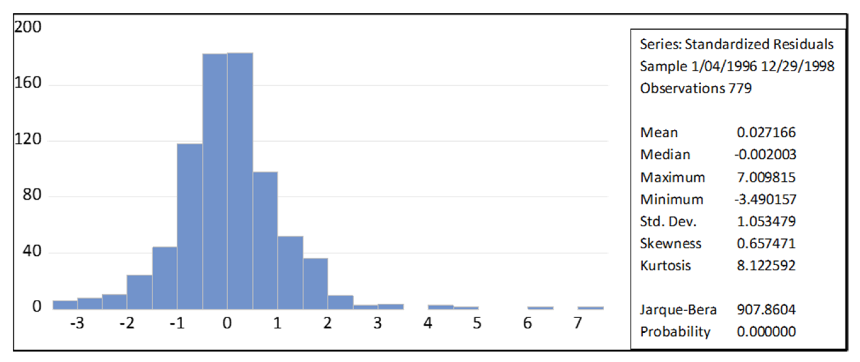
Johansen and Sornette (
2002) analyzed the most important financial indices, currencies, gold, and a sample of individual stocks in the US, finding fat-tails in all series (except for the CAC40). In addition to that, they found that 98% of drawdowns and draw-ups could be fitted to an exponential model, 98% of the time. These 98% could be produced by a financial market following a GARCH process, while approximately 1–2% of the largest drawdowns could not be fitted to the exponential or Weibull functions. This could indicate that the largest drawdowns are outliers, even when most of the time the very largest daily drops are not outliers. An explanation for this could be the emergence of a sudden persistence of consecutive daily drops, with a correlated magnification of the amplitude of drops (
Johansen and Sornette 2002). Their main result was the existence of the emergence of transient correlations across daily returns. These have been found in emerging markets (reflecting the low volume) but also in the October 1987 crash. Such would lead us to analyze the problems related to the extended use of Value-at-Risk (VaR) and extreme value theory (EVT). In the case of VaR, this is focused on the analysis of one-day extreme events happening during a specified timeframe. However, the bigger losses occur due to the emergence of transient correlation, which in turn will lead to runs of cumulative losses. These correlations would make the drawdowns much more frequent than expected when independence between daily returns is assumed. Regarding EVT, if large drawdowns are outliers, extrapolating the tails from smaller values cannot be correct.
Drastic price changes without a change in economic fundamentals could be explained by panicked uninformed traders that sell, causing prices to drop (
Barlevy and Veronesi 2003). However, those sells could be rational if they are acting in response to perceived information that they received from the market. If that is the original cause of crashes, there would not be a need of an exogenous cause.
Eguiluz and Zimmermann (
2000) mention that the occurrence of crashes could be explained by the mechanisms of information dispersion and herding.
Threshold models, where outcomes depend on how people react to other people’s actions, apply to a multitude of situations, including the stock market. These models start with the initial distribution of thresholds and try to estimate how many will end choosing each of the two alternatives presented (
Granovetter 1978); that is, to find the equilibrium that will arise over time. Finding these equilibria is difficult, since people have different thresholds regarding how many people would have to hold an opinion for them to consider changing their own opinion. Threshold models and mimetic contagion processes are related, since these processes can be identified, for as the imitation disseminates, it reinforces itself given that individuals show an increasing tendency to imitate (
Orlean 1989). An opinion shared by a great number of people would be very attractive, increasing the chances that those that ignored it at first, could change their mind.
Devenow and Welch (
1996) mention that influential market participants highlight the high influence that other market participants have in their decisions, which could lead to mimetic contagion whenever there is a bubble or crash.
It has been considered by
Orlean (
1989) that a trader that analyses information considering the Walrasian general equilibrium would decide if this were relevant or not, in an objective way, according to market fundamentals. However, in his framework, the speculator would only consider how other traders think and act, drawing a parallelism between this situation and the beauty contest example created by Keynes. In cases of mimetic contagion, investors are not interested in fundamentals, but only in the information they can obtain from market participants; they could just copy the actions of their neighbors (
Orlean 1989). This could help explain bubbles and crashes, but received little attention since it was considered akin to irrationality. However, when an agent has no information, it could end better off by copying somebody with information, or simply end in the same situation (in case the copied agent has no information).
Between the two extreme positions, where one extreme sees herding as an example of irrational behavior, and the other sees it as an example of rationality, but considers externalities, information, and incentives, there is an intermediate view that holds that decision-makers are near-rational, economizing on information processing or information acquisition costs by using heuristics, and that rational activities by third-parties cannot eliminate this influence (
Devenow and Welch 1996;
Gonçalves et al. 2021).
Orlean’s model is compatible with the model proposed by
Graham (
1999), where there are two types of traders: smart ones, who receive informative signals, and dumb ones, who receive uninformative signals. Given that the smart analysts’ signals are positively correlated, they would tend to act in a similar way, as a consequence, in certain circumstances, an analyst can look smart by herding. On the other hand, an analyst would have a bigger tendency to ignore leaders’ opinions and trust his own personal information if he has a bigger perceived ability (or high confidence). This point of view is shared by
Zhou and Sornette (
2009, p. 869), who add that “it is actually rational to imitate when lacking sufficient time, energy, and information to take a decision based only on private information and processing, that is (…), most of the time”.
Bubbles are more likely to appear in isolated industries or markets (
Krause 2004), given that analysts and traders in the sector are usually interacting amongst themselves most of the time, and that those industries or markets could be not well integrated into the rest of the economy, magnifying the effects of biases.
Johansen and Sornette (
1999b) mention that traders do not maintain a fixed position with respect to their colleagues, instead they are in constant change, creating new interactions and correlations.
The effects of herding behavior in financial markets can be seen as positive or negative feedback mechanisms causing price accelerations or decelerations and (anti)-bubble formation, where asset prices become detached from the underlying fundamentals (
Bastiaensen et al. 2009). This phenomenon is closely related to the concept of positive and negative feedbacks; the latter tend to regulate systems towards an equilibrium, while positive feedbacks make high prices or returns even higher (
Sornette 2003). In the stock market’s context, positive feedback would be referred to as trend-chasing (
Johansen and Sornette 1999b); however, it is also noted that, at some point, not only technical analysts but also fundamentalists will have to act as trend-chasers to increase benefits. Positive feedbacks, caused among others by derivative hedging, portfolio insurance, and imitative trading, are considered an essential cause for the appearance of non-sustainable bubble regimes. Specifically, the positive feedbacks give rise to power law (i.e., faster than exponential) acceleration of prices (
Zhou and Sornette 2009).
Using tools to quantify the degree of endogeneity, it has been determined that it has increased from 30% in the 1990s to at least 80% as of today, showing that due to technological advances that make possible to trade several times in a short period of time, we develop bubbles and crashes that can develop and evolve increasingly over time scales of seconds to minutes (
Sornette and Cauwels 2014).
3. The Model: The Log-Periodic Power Law (LPPL)
The proposed framework, following
Lin et al. (
2014),
Li (
2017), and
Ko et al. (
2018) considers the existence of two types of traders: Perfectly Rational Investors (Fundamental Value Investors) with rational expectations, and Irrational Traders (Trend Followers/Noise Traders/Technical Traders that exhibit herding behavior). From their interaction we develop the characteristic periodic oscillations in the stock market that are visible in the logarithm of the price in periods before crashes. These oscillations will provide evidence towards the increasingly greater frequencies that eventually reach a point of no return, where the unsustainable growth has the highest probability of ending in a violent crash or gentle deflation of the bubble (
Yan et al. 2011). In a crash, “there is a steady build-up of tension in the system (…) and without any exogenous trigger a massive failure of the system occurs. There is no need for big news events for a crash to happen” (
Bastiaensen et al. 2009, p. 1).
Accelerating prices at the end of bubbles occurs due to the higher the probability of a crash, the faster the price must increase (conditional on having no crash) (
Johansen et al. 2000). This happens since investors expect higher prices in order to be compensated for the higher risk of a crash. That way prices are driven by the hazard rate of a crash, defined as the probability per unit of time that the crash will happen in the next instant if it has not happened yet (
Johansen et al. 2000). We will represent the hazard rate conditional on time as
h(t). The higher the hazard rate, the higher the price, since this is the only result consistent with rational expectations.
Two characteristics of critical systems have been observed in the stock market by
Johansen et al. (
2000): “(a) local influences [that] propagate over long distances that makes the average state of the system very sensible to small perturbations (that is, it becomes highly correlated) and (b) self-similarity across scales at critical points where big concentrations of bearish traders may have within it several islands of traders who are mostly bullish, each of which in turn surrounds lakes of bearish traders with islets of bullish traders; the progression continues all the way down to the smallest possible scale: a single trader” (
Johansen et al. 2000, p. 234).
Local imitation cascades through the scales into global coordination due to critical self-similarity (
Johansen et al. 2000). Given that similar crashes have happened during this century, we will have to consider that maybe it is the structure of markets that leads to crashes, since almost everything else have changed during the years. The origin of the crashes could lay on the organization of the system itself (
Johansen and Sornette 1999a).
According to
Crutchfield (
2009), when you add intelligence to a group, this starts to behave in more complicated ways, since agents try to anticipate each other creating oscillations in the market; something that would not happen with simple agents without big memories or complex strategies. He concludes that dynamical systems consisting of adaptive agents typically do not tend to a mutually beneficial global condition—they cannot find the Nash Equilibrium. The lesson is that dynamical instability is inherent to collectives of adaptive agents.
Traders are inserted inside a network of contacts, and it is from these interactions that they will be influenced and take decisions, either buy or sell. Traders tend to imitate their closest neighbors; in periods where imitation is high, there would be an increased order in the market (e.g., people agreeing to sell), and that would lead to a crash (
Johansen et al. 2000). However, the normal state of the market is a disordered one where buyers and sellers disagree with each other and roughly balance each other out (
Johansen et al. 2000). Despite the usual characterization of chaos as something negative, it is the predominance of order that brings bubbles and crashes to the market.
Another dynamical explanation of the emergence of oscillatory patterns in prices considers the competition between positive feedback (self-fulfilling sentiment), negative feedbacks (contrarian behavior and fundamental value analysis) and inertia (everything takes time to adjust) (
Zhou and Sornette 2009). According to the later, the competition between these market participants, plus the effect of inertia, would lead to nonlinear oscillations approximating log-periodicity. Another point to have in mind, as to what provokes the log-periodic behavior, is the fact that most investment strategies followed by trend followers are not linear, they tend to under-react for small price changes and over-react for large ones (
Ide and Sornette 2002).
The log-periodicity observed in the stock market before crashes has been interpreted as “the observable signature of the developing discrete hierarchy of alternating positive and negative feedbacks culminating in the final ‘rupture’, which is the end of the bubble often associated with a crash” (
Zhou and Sornette 2009, p. 870).
Initial crash rates are exogenous, and investors receive this information and translate it into prices. Later, there could be (or not) a feedback between agent actions and the hazard rate. The crash itself is an exogenous event, even when everybody knows that it could be coming, nobody knows exactly why, so even when they can be compensated for it in the form of high prices, they cannot obtain abnormal returns (after adjusting risk) by anticipating the crash (
Johansen and Sornette 2002). However, the specific way the market collapsed is not the most important problem, since a crash occurs due to the market entering an unstable phase, and any small disturbance or process may trigger the instability (
Sornette 2003). Once a system is unstable, many situations could trigger the reaction (the crash), and as such that is why sometimes it is so difficult to find the exact origin of a crash, and many different news points could be indicated as the origin of the crisis, even when the real origin was that the hazard rate was already high and the log-periodic price oscillations had no room to keep accelerating.
It has been suggested by
Sornette and Johansen (
1997, p. 420) that “the market anticipates the crash in a subtle self-organized and cooperative fashion, hence releasing precursory ‘fingerprints’ observable in the stock market prices.” They consider that there is information to be picked up by investors from prices; however, this subtle information has not been discovered by most.
Specific events can act as revelators rather than the deep sources of the instability (
Johansen et al. 1999). Even political events can be considered revelators of the state of a bigger dynamical system in which the stock market is included. Endogenous crashes can be understood as the natural deaths of self-organized, self-reinforcing, speculative bubbles giving rise to specific precursory signatures in the form of log-periodic power laws accelerating super-exponentially (
Johansen and Sornette 2010). However, there have been some exogenous crashes identified. In those cases, crashes can be related to some extraordinary events (
Johansen and Sornette 2010).
The LPPL Equation
The Log Periodic Power Law (LPPL) equation used in this document has been dubbed the “Linear” Log-Periodic Formula (even when it is not linear):
where
tc = critical time,
ω = log-periodic angular frequency,
ϕ = phase,
β = exponent, and other important quantities that do not appear in the equation are
tfirst and
tlast, which represent the first and last data point used for the fit.
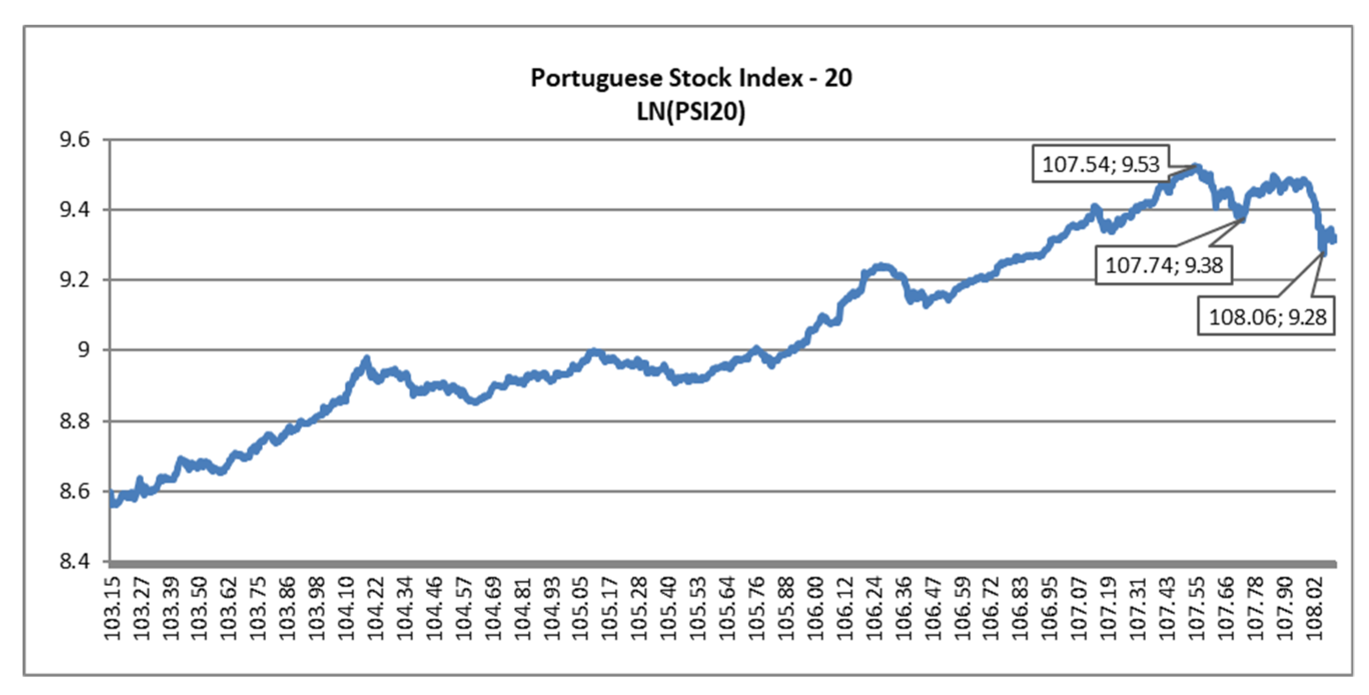
Originally, the LPPL equation, designed to predict the critical time, used the market index as a measure of the level of the market. However, to avoid getting distorted signals due to the exponential rise of price (and avoiding the need to de-trend and getting additional distortion), the logarithm of the index was preferred (
Sornette and Johansen 1997). Another advantage of this specification is due to investors being concerned with relative changes in stock prices rather than absolute changes (
Feigenbaum 2001). Correct specification depends on the initial assumptions regarding the expected size of the crash. If we expect it to be proportional to the current price level, we would need to use the logarithm of the price (preferred for longer time scales, such as eight years). However, if we expect the crash to be proportional to the amount earned during the bubble, the price itself should be used. This could be better suited for shorter time scales, such as two years (
Johansen and Sornette 1999a).
An interesting relationship is:
which represents the ratio of consecutive time intervals. This is important since it is a constant and permits us to identify the oscillations that contain the critical date
tc. This is possible since the time intervals tend to zero at the critical date and complete it in a geometric progression (
Johansen et al. 1999). A curious observation with regards to
λ is that it tends to be around two in a wide variety of systems, including growth processes, rupture, and earthquakes (
Sornette 1998). In this representation, ω is encoding the information on discrete scale invariance, and thus is on the preferred scaling ratio between successive peaks.
With regards to
tc, we can say that it is determined by initial conditions (
Johansen and Sornette 1999a) and marks the estimated end of a bubble, which could take the form of a significant correction or a crash 66% of the time (
Zhou and Sornette 2009). However, there is a finite probability of a phase transition to a different regime (without a crash), such as a slow correction. This finite probability is given by:
It is important to stress the residual probability for the coherence of the model, since otherwise agents would anticipate the crash and not remain in the market (
Johansen and Sornette 1999b).
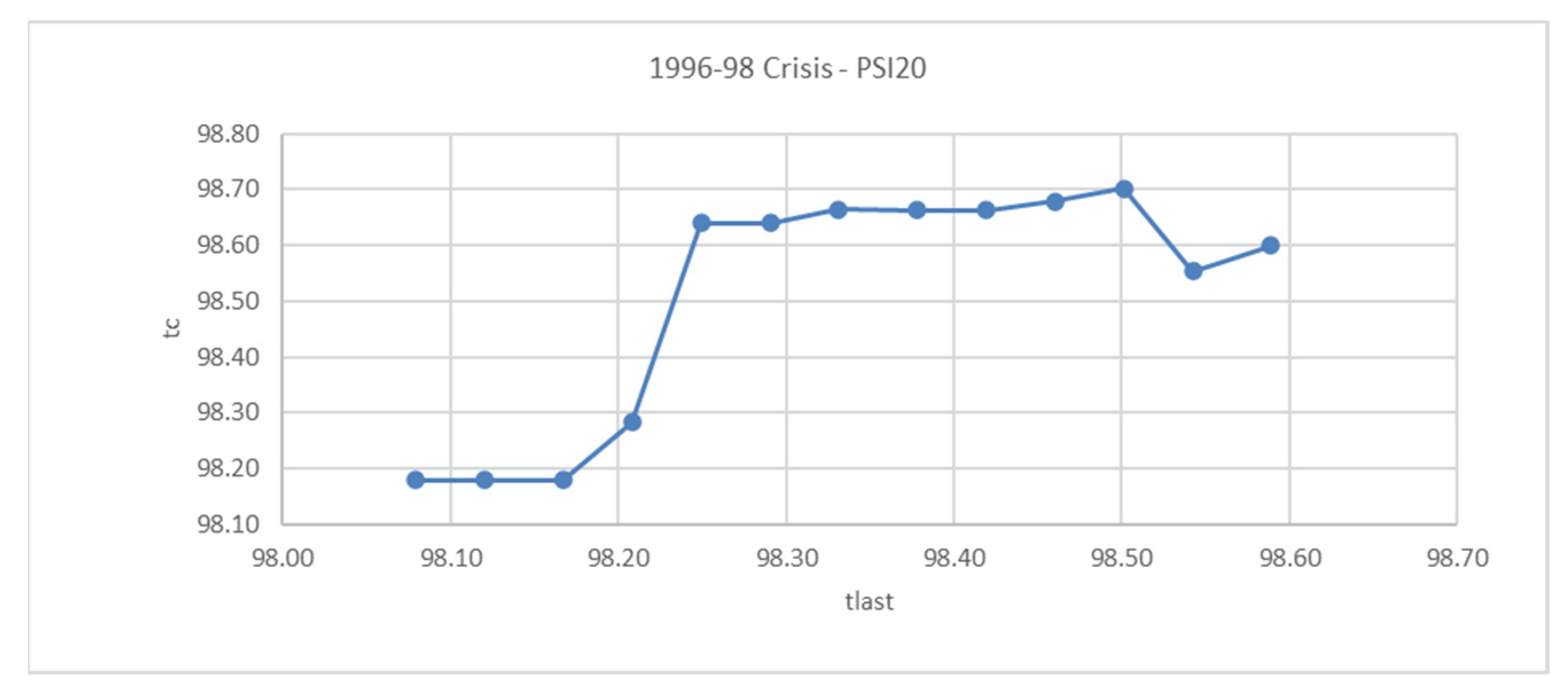
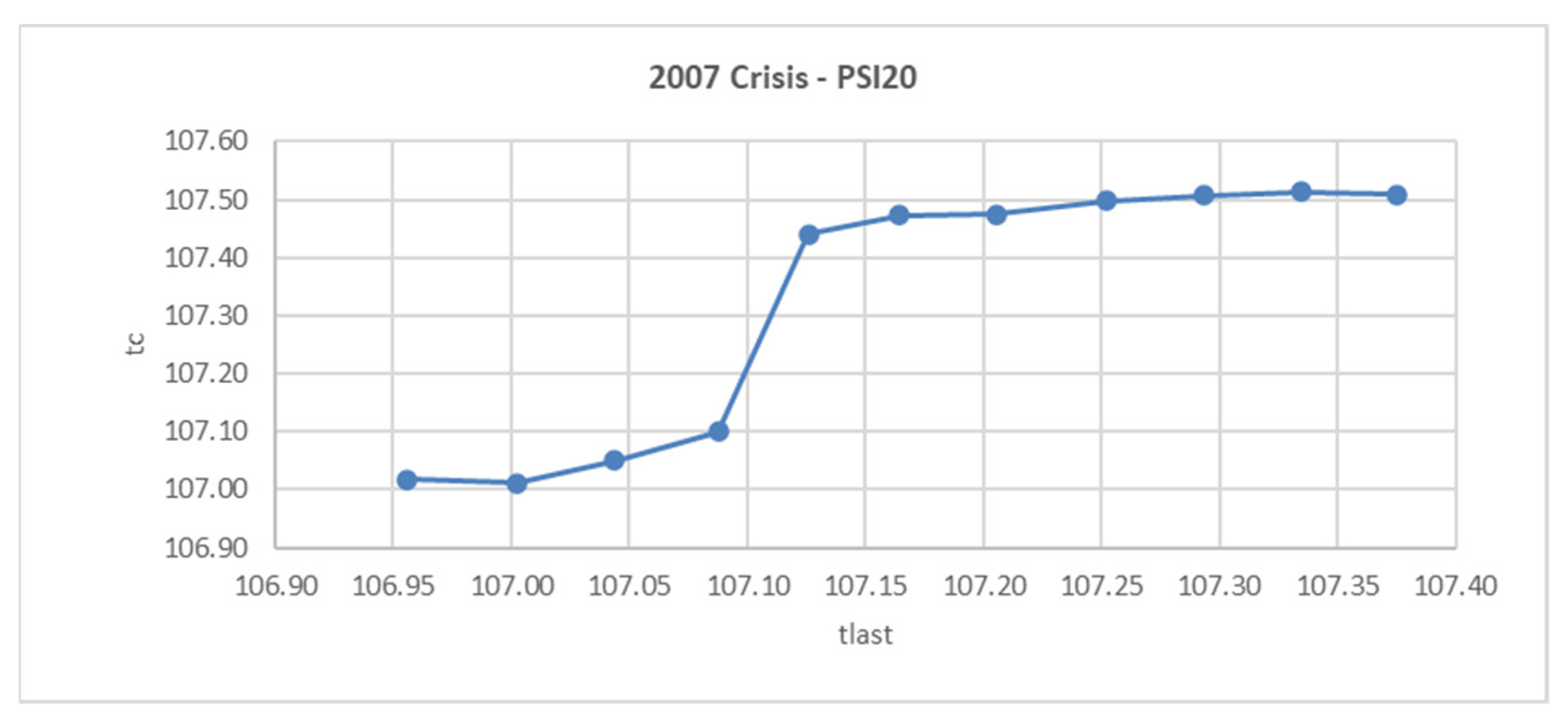
Tests of sensitivity and robustness found that
tc and
ω are very robust, with respect to the choice of the starting time (
tfirst) of the fitting interval (
Zhou and Sornette 2009). They found similar results analyzing the sensitivity of
tlast. These results confirmed that fits are robust and predictions reliable.
Using parameters obtained from fitting the LPPL equation (
tc and
ω), it is possible to calculate the number of oscillations (represented as
Nosc) appearing in the time series by using an equation presented by
Zhou and Sornette (
2009):
Zhou and Sornette (
2009) mention that multiplicative noise on a power law accelerating function has a most probable value of
Nosc ≈ 1.5, and that, if
Nosc ≥ 3, we can reject with 95% of confidence that the log-periodicity observed comes from noise.
To model LPPL equation, we will use the usual restrictions suggested by
Sornette (
2004):
(The exponent needs to be between 0 and 1, in order to accelerate and to remain finite, but we will use a more stringent suggested range):
(This corresponds to 1.5 <
λ < 3.5):
After fitting the Portuguese stock market index to the LPPL equation, it could be expected to obtain reasonable fits with low errors, as well as post-dictions of critical dates close to the real observed dates. However, it would be unrealistic to expect that the predicted
tc coincides exactly with the time of the crash, since the not fully deterministic nature of crashes (
Johansen et al. 2000). Another point considered by the latter is that false alarms could be unavoidable, but most endogenous crashes will be predicted. As a way to calculate the significance of the values for
β and
ω in the usual range,
Johansen and Sornette (
1999a) analyzed 400-week random intervals from 1910 to 1996 of the Dow Jones average and tried to fit the log-periodic equation. They only were able to find six data sets in the usual ranges, and all corresponded to periods before crashes: 1929, 1962, and 1987. These results strengthened the case for the reliability of this method of analysis.
Regarding the log-periodic angular frequency, a fundamental has been identified in a different analysis in the range
ω1 ≈ 6.4 ± 1.5, with other peaks having been found on its harmonics:
However, even when the importance of the harmonics is expected to decrease exponentially,
ω2 and
ω3 have been observed to be very significant, with this being something more prevalent in individual stocks rather than in aggregate indexes, due to the additional noise of the data (
Zhou and Sornette 2009).
6. Conclusions
Bubbles and the way these develop have been presented in different markets during different eras showing common features, despite technological changes or differences among countries. In all cases, when the bubble ends analysts would look for what caused the crash, and they will usually use hindsight some piece of news. However, it seems to be that financial markets are unstable by design, and that the oscillations of prices before crashes could be caused by the way markets are organized. It is possible that the cause of the crashes are the bubbles itself, and the news are just triggers, but the instability must exist to begin with.
In this work, we present the theory of self-similar oscillatory finite-time in finance and its application to the prediction of crashes. First, we discussed some terms and concepts, followed by a brief introduction to the theory, to analyze its different aspects and the challenges concerning the prediction aspect.
We test the Log Periodic Power Law/Model (LPPM) to analyze the Portuguese stock market in its crises in 1998, 2007, and 2015. Parameter values were in line with those observed in other markets. The model performs robustly for Portugal, which was a small market with liquidity issues and the index was only composed of 20 stocks. Thus, we provided consistent evidence in favor of the proposed LPPM methodology.
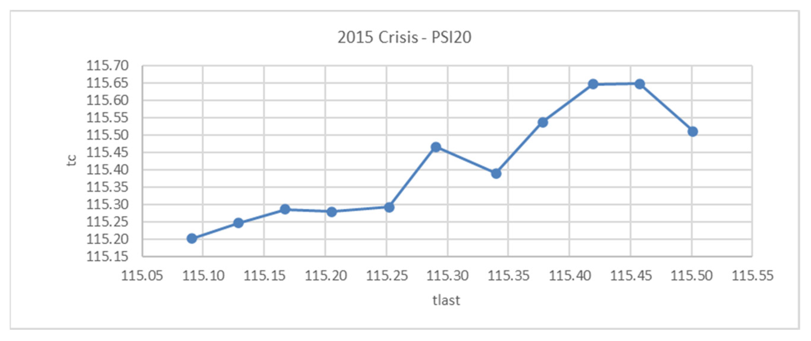
The LPPM methodology proposed here would have allowed us to avoid big loses in the 1998 Portuguese crash, and would have permitted us to sell at points near the peak in the 2007 crash. In the case of the 2015 crisis, we would have obtained a good indication of the moment where the lowest data point was going to be achieved.
Predictions of critical time appeared to be stable, regarding the last data point included. We obtained a string of values of tc surrounding some specific number consistent with real data. The number of oscillations required to verify that the log-periodicity was not coming from noise (Nosc = 3) signaled robust results that assured to take into consideration results from the model.
Parameter values were in line with those observed in other markets. Regarding the fitting procedure, the minimization of SRSD or RMSD led to similar results. By using artificial series, we were able to provide a measure of how stable are our critical time predictions relative to small perturbations, and to generate bands that could be expected to land around the real critical time.
Altogether, these results supported the potential of our approach to study bubbles and crashes. If the model performed robustly for Portugal, which was a small market with liquidity issues and the index was only composed of 20 stocks, then our evidence provided consistent support in favor of the proposed LPPM methodology.
The use of LPPM methodology could be helpful in order to prevent major losses in diversified stocks portfolios, whenever we are at a bubble situation. LPPM can help to identify in advance the signs of a bubble that are becoming increasingly instable and that can blow to any unexpected trigger. This is of relevance for policy makers and market supervisors, in the sense that it can help to implement risk mitigating actions.
Expectably, we can also apply LPPM to smaller crashes.
Baker et al. (
2021) used small ranges of variation (+/−2.5%) to identify small but out of ordinary jumps. It is relevant to test LPPM in smaller crashes and investigate eventual differences. LPPM can be extended to other phenomena. For example, it can be applied to individual stocks. In this case it is necessary to remember that the series are going to be much noisier, and it could be necessary to allow more degrees of freedom for the parameters to achieve a good fit. Given that Log-Periodic Analysis can be applied to the Gross National Product, a joint analysis of both conditions can be undertaken.
Our research is limited to the study of critical crashes in the Portuguese stock market during the latest three crisis. Our results could be extended to study the impact of COVID-19 induced stock returns. The data is still difficult to analyze, in the case of Portuguese market, since it is unclear whether we have reached the critical point. Further research can look at the predictive ability of LPPM in this context.


 ,
, 


