A Machine Learning Pipeline for Forecasting Time Series in the Banking Sector

Abstract

The problem of forecasting time series is very widely debated. In recent years, machine learning algorithms have been very prolific in this area. This paper describes a systematic approach to building a machine learning predictive model for solving optimization problems in the banking sector. A literature analysis on applying such methods in this particular area is presented. As a direct result of the described research, a universal scenario for forecasting various non-stationary time series in automatic mode was developed. The developed scenario for solving specific banking tasks to improve business efficiency, including optimizing demand for ATMs, forecasting the load on the call center and cash center, is considered. A machine learning methodology in economics that can yield robust and reproducible results and can be reused in solving other similar tasks is described. The methodology described in the article was tested on three cases and showed the ability to generate models that are superior in accuracy to similar predictive models described in the literature by at least three percentage points. This article will be helpful to specialists dealing with the problem of forecasting economic time series and students and researchers due to a large number of links to systematic literature reviews on this topic.

1. Introduction

In recent years, the banking service market has been characterized by the development of an ATM network, since in the modern world, ATMs are considered one of the priority ways to distribute banking services and expand the client portfolio, which is an excellent advantage for any bank. A truly ramified network of ATMs is not only one of the practical tools for developing the infrastructure of the retail business but also contributes to a significant increase in the bank’s profitability.

Time series modeling is a fairly popular area in the banking sector. One of these tasks is the problem of predicting the optimal amount of loaded cash in ATMs with proper planning and cash flow management. It is possible to minimize the costs of servicing cash flows, for example, by increasing the interval between ATM collections (collection period), to reduce the costs of collector services and to relieve the cash departments.

Moreover, the sudden use of all cash in ATMs leads to downtime, reducing the efficiency of using the ATM network and, consequently, the bank’s profit. However, along with developing a network of ATMs for working with cash, additional problems include loading cash, choosing the denomination of the notes required for issuing, choosing the desired currency, and routing the accepted notes. Due to many objects of forecasting, there is an acute issue of developing a universal algorithm and forecasting methodology. The application of a time series methodology adequately reflects the construction of the model when solving the problems of analysis and forecasting in the ATM network. This article proposes a method and shows its application to several tasks.

2. Related Work

Many studies are devoted to applying machine learning methods for problems of forecasting time series. The most developed areas of application include stock market forecasting (Aliev et al. 2004), trading system development (Dymowa 2011), and practical examples of market forecasting (Kovalerchuk and Vityaev 2006) using machine learning models. Bahrammirzaee (2010) reviewed research on financial forecasting and planning and other financial applications using various artificial intelligence techniques such as artificial neural networks (ANNs), expert systems, and hybrid models.

For example, evolutionary algorithms find many applications in forecasting economic and financial time series (Chen 2002); multipurpose evolutionary algorithms have been widely studied for various economic applications, including time series forecasting (Tapia and Coello Coello 2007; Ponsich et al. 2013; Aguilar-Rivera et al. 2015). Li and Ma examined implementations for stock price forecasting and some other financial applications (Li and Ma 2010). Tkáč and Verner (2016) investigated various implementations of ANN in financial applications, including for predicting stock prices. Recently Elmsili and Outtaj investigated applications of ANNs in economic and management research, including series forecasting (Elmsili and Outtaj 2018).

There are many systematic reviews on specific applications of financial time series forecasting. The dominance of forecasting financial and stock markets is traced in this area. Several predictive stock market research reviews have been published based on various soft computing methods at different times (Nair and Mohandas 2014; Cavalcante et al. 2016; Atsalakis and Valavanis 2009). Chatterjee et al. (2000), Katarya and Mahajan (2017) focused on ANN-based financial market predictive studies, while (Hu et al. 2015) focused on machine learning (ML) implementations for inventory forecasting and algorithmic trading models. In another application for time series forecasting, researchers have reviewed studies on forex forecasting using ANN (Hewamalage et al. 2021) and various other soft computing methods (Pradeepkumar and Ravi 2018).

Note that in all the variety of financial and economic applications of time series forecasting methods, insufficient attention is paid to more specific problems (Sezer et al. 2020), such as forecasting the ATM load, which is the subject of this article. However, this does not mean that this problem has not been considered in the literature (Ekinci et al. 2019). We note, for example, the works of M. Rafi, which are devoted to modeling ATM loading using classical statistical methods such as moving average autoregression (Rafi et al. 2020) and the use of recurrent neural networks based on LSTM cells (Asad et al. 2020). LSTM can generally be considered a classical method since it was created specifically for modeling time series. Therefore, it often finds application in this problem (Arabani and Komleh 2019; Serengil and Ozpinar 2019; Rong and Wang 2021). Also, classical and deep learning methods were applied to this problem, the performance comparison of which are given in Vangala and Vadlamani (2020) and Hasheminejad and Reisjafari (2017). However, an analysis of the literature shows that classical machine learning methods such as regression analysis (Rajwani et al. 2017), support vector machines (Jadwal et al. 2018), dynamic programming (Ozer et al. 2019), ARIMA (Khanarsa and Sinapiromsaran 2017), and gradient boosting (Shcherbitsky et al. 2019) are used much more often.

Mention should be made of the research work carried out based on the database of the NN5 competition (Adeodato et al. 2014), since this competition is very closely related to our work. The dataset in this competition contains two years of daily cash withdrawals from 111 ATMs in the UK. The challenge is to predict ATM withdrawals for each ATM over the next 56 days.

The most efficient model, from Andrawis et al. (2011), an ensemble of general Gaussian regression, neural network, and linear models, achieved a SMAPE of 18.95%. The article by Venkatesh et al. (2014) improved the prediction accuracy of Andrawis et al. (2011) by clustering similar ATMs and applying many popular neural networks. These studies show that modern ML algorithms for forecasting time series produce results better than classical methods. Also, one of the advantages of that work is taking into account the particular clusters to which an ATM belongs, which improves the quality of the demand forecast.

In another work, Kamini et al. (2014) further improved the results by simulating chaos in cash withdrawal time series and referring to popular neural network architectures. However, the study did not include the effects of exogenous traits, such as the “day_of_week” dummy, whether it is a weekday or a weekend, as these traits significantly impact forecast accuracy. Information regarding whether the day corresponds to a working day or a weekend is relevant to the problem under study.

Ekinci et al. (2015) considered the problem of optimizing ATM cash replenishment in Istanbul using simple linear regression with grouping. They have achieved a MAPE score of 22.69% on average. Catal et al. (2015) used the same dataset, NN5, as the aforementioned papers and exponential smoothing to achieve the average SMAPE of 21.57%.

None of the articles reviewed above discuss the importance of identifying and marking periodic anomalies in time series related to optimizing the management of cash flows in bank ATMs. However, the correct marking of periodic anomalies is necessary for the efficient generation of the feature space and to build a predictive model. This is one of the critical points in this work—considering the influence of periodic anomalies associated with regularly recurring events. However, Fremdt (2015) explores the methodology for detecting anomalies in time series using the CUSUM method and shows its applicability to financial data (value of stock prices). Therefore, the results obtained by Fremdt in the article on marking anomalies by this method is applicable in this work.

3. Problem Statement

Historically, the classical time series methods have been econometric models such as AR, MA, ARMA, ARIMA, SARIMA, exponential smoothing, triple exponential smoothing, e.g., (Katarya and Mahajan 2017; Sezer et al. 2020; Arabani and Komleh 2019).

Several disadvantages characterize these models. Although the models of the autoregressive class (ARIMA and its modifications) show pretty good quality in solving real problems, there are serious shortcomings which prompted the need to develop other methods that compensate for the shortcomings of the previous ones. The following disadvantages can be distinguished:

(1)

The predictive period. A significant drawback of some models is that the prediction period is limited to a few points, which is unacceptable in the absolute majority of applied problems (Andrawis et al. 2011).

(2)

Data preprocessing and preparation. Autoregressive models are based on the assumption that the original time series is stationary, which contradicts reality in actual data. As a result, researchers have to spend much time making the time series stationary for such models. This problem is especially acute when the number of time series exceeds hundreds and thousands. Respectively, it becomes difficult to look for a way to make each time series stationary (Draper and Smith 1998; Yohannes and Webb 1999).

(3)

Computational complexity. Almost all the models listed above need to select a certain number of parameters, and the more complex the model, the more parameters in it need to be tuned (Draper and Smith 1998; Yohannes and Webb 1999; Morariu et al. 2009). Consequently, this imposes limitations on the performance of the forecasting system itself.

Table 1 provides a comparison of time series forecasting models by several criteria (Andrawis et al. 2011; Venkatesh et al. 2014; Draper and Smith 1998; Morariu et al. 2009).

Table 1. Comparison of time series forecasting models.

Criteria	Regression	Autoregressive	Exp. Smoothing	Decision Trees	Neural Network
Flexibility and adaptability	+	−	−	+	−
Ease of choice of architecture, the need to select parameters	+	+	−	−	−
Ability to simulate nonlinear processes	−	−	+	+	+
Model learning rate	+	−	−	+	−
Consideration of categorical features:	−	−	−	+	+
Training set requirements	N	ND	N	−	N

Table 1. Comparison of time series forecasting models.

Criteria	Regression	Autoregressive	Exp. Smoothing	Decision Trees	Neural Network
Flexibility and adaptability	+	−	−	+	−
Ease of choice of architecture, the need to select parameters	+	+	−	−	−
Ability to simulate nonlinear processes	−	−	+	+	+
Model learning rate	+	−	−	+	−
Consideration of categorical features:	−	−	−	+	+
Training set requirements	N	ND	N	−	N

Where:

• N—denotes that data should be normalized.
• S—denotes that it is required to bring the series to a stationary form.

The criterion “Flexibility and adaptability” means:

• “+”—models are flexible and adapt when the distribution of the target value changes1;
• “−”—models are inflexible and do not adapt with a sharp change in features because they are tied to the parameters of seasonality. With a sharp change in the distribution of the target value, retraining is required.

The criterion “Ability to simulate nonlinear processes” means:

• “+”—non-linear connections are taken into account.
• “−”—linear relationships only.

The criterion “Model learning rate” means:

• “+”—fast (comparable to SVM in computational complexity).
• “−”—the method is computationally intensive (comparable to ANN in complexity).

The criterion “Consideration of categorical features” means:

• “+”—taken into account. No conversion required.
• “−”—not taken into account, it is required to carry out transformations (for example, One-hot-encoder2 or label encoder3).

Based on the comparative analysis of the data of model approaches, it can be concluded that there is no uniform approach to forecasting all types of time series. The methods used differ for stationary and non-stationary time series. The choice of a model is often based on a preliminary visual assessment of the data in question. If a time series has a trend, then regression models show the best predictive ability, and exponential smoothing models show the best predictive ability for series with a pronounced seasonality.

Given the specificity of time series in the banking sector, such as their non-stationarity for the most part, as well as their large number, it is necessary to apply forecasting methods based on modern machine learning (decision trees, random forest, gradient boosting over decision trees, neural networks).

These methods will solve several problems in forecasting time series in the banking sector. First, there is no need to waste time converting the original series to a stationary form. Secondly, given a large number of time series (for example, each time series for a separate ATM, and there are many such ATMs, approximately 200,000), we claim that it is possible to create a universal pipeline applicable to forecasting a large number of time-series.

Thus, this study aims to optimize the management of cash flows in bank ATMs. The primary solution method is the development of a universal methodology for automating the stages associated with the automatic generation of the feature space, anomaly detection, selection of hyperparameters, and training models. In conducting this research, a software product in Python was developed. We have used a sample of observations of a behavioral model of an ATM for 2016–2019 as the training dataset to test the resulting model. The application of the developed approach was tested on several cases with the interpretation of the importance of the features of the models making it possible to determine the strength and influence of each of the features of the forecast.

4. Methods

The specific stages described below that make up the predictive model production methodology were developed following the staging of typical machine learning projects designed to solve similar problems. Examples of describing the stages of data analysis for creating predictive models can be seen in previous studies (Morariu et al. 2009; Bahrammirzaee 2010; Li and Ma 2010; Nair and Mohandas 2014; Katarya and Mahajan 2017; Sezer et al. 2020; Asad et al. 2020; Arabani and Komleh 2019; Kamini et al. 2014). A universal pipeline for forecasting time series was developed to solve the problem of forecasting, consisting of the following steps:

4.1. Formation of a Feature Space

For any machine learning algorithm, a feature space is required. An extensive feature space typical for time series includes:

• One-hot encoding of calendar features (day of the week, month, weekend, holiday, reduced working day, etc.).
• Lagged variables (time series values for previous days).
• Rolling statistics grouped by calendar features (average, variance, minimum, maximum, etc.).
• Events of massive payments (advance payment, salary, etc.).

The selection of the necessary parameters (window width in statistics, the number of lags) and the selection of significant features are performed for each time series individually using cross-validation in a sliding window.

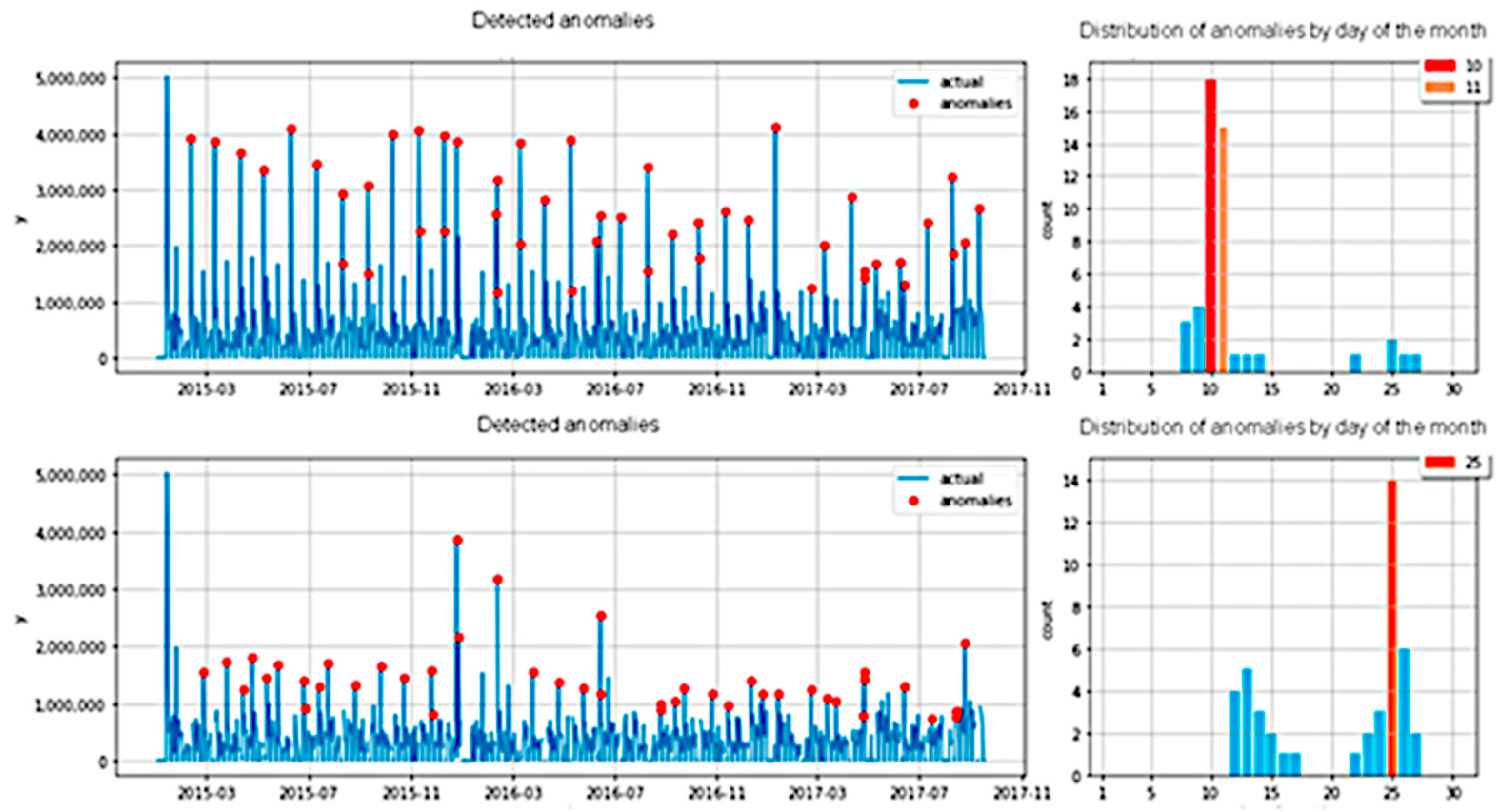
4.2. Anomaly Detection

Anomaly detection plays an essential role in time series analysis and forecasting. Training on a time series with many outliers can significantly reduce the prediction accuracy.

Anomalies can be classified into two types:

• Periodic anomalies.
• Anomalies that do not have a periodicity.

The first class can be used as an element of the feature space for further forecasting, while the second can be excluded from the sample.

CUSUM (cumulative sum) is a method that tracks variations in a process (time series) (Aue et al. 2012). It is based on the accumulation of changes in the time series from the mean. As soon as the cumulative sum exceeds the specified threshold value, this point is marked as an anomaly. The detection process is carried out through iterative learning and prediction with a moving window (Fremdt 2015). The method parameters indicated below are calculated on the training set, and anomalies are detected on the test set.

Mathematical interpretation:

$$\begin{gathered} S_i^{+}=\left(0, S_{i+1}^{+}+x_i-\left(\mu +drift\ast \sigma \right)\right) \\ {S}_i^{-}=\left(0, S_{i-1}^{-}+x_i-\left(\mu -drift\ast \sigma \right)\right) \\ Anomalies=\{1 if S_i^{+}>threshold·\sigma or S_i^{-}<-threshold·\sigma , 0 otherwise \end{gathered}$$

where:

• $S_i^{+}$—the upper limit of the cumulative sum.
• $S_i^{-}$—the lower limit of the cumulative amount.
• $x_i$—values of the time series in the test window.
• $\mu$—the average of the time series in the learning window.
• $\sigma$—standard deviation of the time series in the learning window.
• $drift$—is the number of standard deviations to summarize the changes.
• $threshold$—the number of standard deviations for the threshold value.

The CUSUM anomaly detection algorithm also helps to identify periodic emissions determined by the days of massive payments: salary, advance payment, pension, etc., and its recursive application in a sliding window helped us to extract significant and relevant signs of relevant events.

Proper labeling of the periodic anomalies is necessary for efficient generation of the feature space for the subsequent construction of a forecast. For example, we analyzed the actual values of the demand sums by days of the month for three years for two ATMs. The visualization of anomalies and their distribution is shown in Figure 1.

Figure 1. Visualization of anomalies and their distribution by day of the month.

For many anomalies, the noise in the search for periodic values is weaker than the signal. The first anomalies were marked as the transfers (weekends, holidays) and were removed from the original series. Then the search algorithm was rerun.

In this problem to be solved, it was revealed that the peak values of the anomalies were on the 10th and 11th of each month, which were interpreted as salary days. There was also a less pronounced anomaly on the 25th. This was explained by the fact that this is an advance, significantly less than the basic salary.

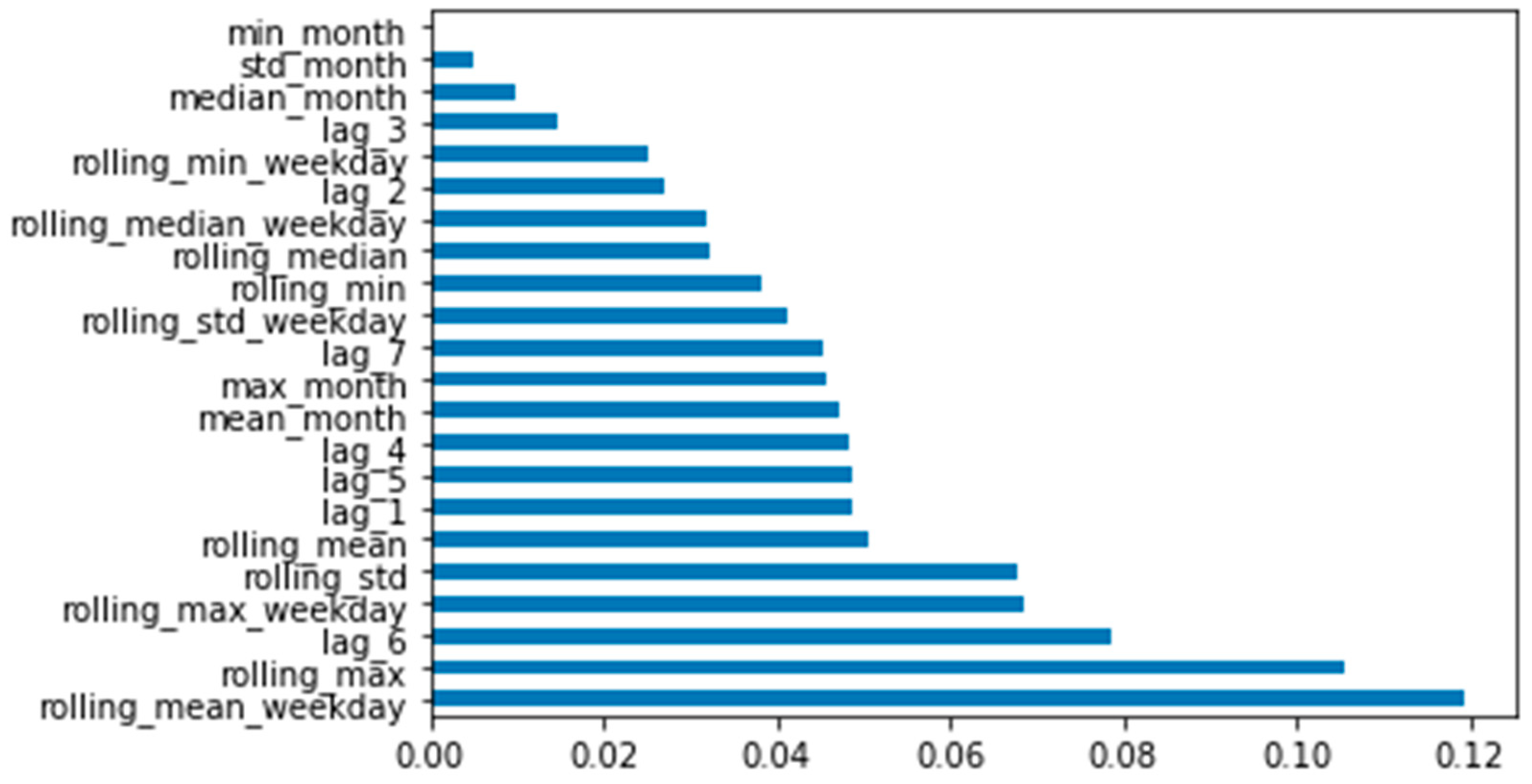
4.3. Feature Selection

Feature selection is performed in a greedy way (Das and Kempe 2011). All possible subsets of the feature space were enumerated. In this case, all possible subsets of the feature space were considered and 2ⁿ⁻¹ options were obtained (without an empty set). It is worth noting that such a feature selection method is computationally laborious. Therefore, parallelization of computations for all processors is built into this method.

When selecting features, cross-validation was used for the time series, the central meaning of which was sequential movement along with the time series, increasing the training sample. In this case, the number of folds for dividing the sample was taken as being equal to five. As a result, we obtained a histogram of the importance of features, where the x-axis was the contribution and influence of each feature on the forecast, and the y-axis lists the features that affected the forecast (Figure 2).

Figure 2. Histogram of the importance of features (see Table 2).

It can be seen from the histogram that the larger the value, the more influential the feature is in the model. The selection of features was carried out by maximizing the objective function of the error for all possible combinations of features. In problems with a small number of features, this technique is a reasonable choice since it allows one to select the most optimal set of features in the foreseeable computational time. Of course, with an increase in the number of features in the initial data, this method becomes inapplicable due to its exponential asymptotics.

This feature selection technique is resistant to a specific set of features in the input data and therefore was preferred as the most universal.

4.4. Building Models

Models based on ensembles of decision trees are used to build forecasts using a random forest and gradient boosting over decision trees. The models were implemented using the sklearn, xgboost, lightgbm, and catboost libraries (Lundberg and Lee 2017; Slack et al. 2020). The choice of the best modeling method was carried out for a given time series in cross-validation.

For most machine learning problems, it is customary to assert the independence of observations. However, for a time series, this assumption about the independence of observations is incorrect since the subsequent values of the series depend on the previous values. Therefore, the cross-validation process for time series is different. The model is trained at some interval of the series from the initial point of the series in time to some value of t. Then a forecast is made for the horizon n. For the interval of the series from t to t + n, the error on this fold is calculated.

Further, the training sample increases from the starting point of the series to the point t + n. Forecasting is carried out for the horizon n, that is, for the series interval from t + n to t + 2 × n and so on until the end of the sample is reached. The number of folds is calculated as the number of row intervals n that fit from the start to the end of the row. This approach is commonly referred to in the literature as “sliding window cross-validation” (Cerqueira et al. 2020).

4.5. Selection of Hyperparameters

It is necessary to select hyperparameters to improve the quality of predictive models. A grid is set to select the optimal values of hyperparameters (Cartesian product of all fitted parameters). The selection method is carried out to select the combination that gave the best quality in the cross-validation sample. This approach has traditionally been used in machine learning and is called grid search (Claesen and De Moor 2015). However, this approach is computationally laborious regarding time and memory, especially if the number of objects for forecasting is too large since it must retrain the model for the entire sample at each iteration. Also, this approach does not consider the results of previous iterations.

Another approach to selecting hyperparameters is the application of Bayesian optimization (Baptista and Poloczek 2018). It should be noted that this approach has shown itself well in practice. The essence of this approach lies in the fact that the best hyperparameters are predicted and selected based on the experiments already carried out, and not just the given values of the hyperparameters are enumerated.

So, as the first step, let us assume that the quality of the model is a Gaussian process from hyperparameters. The initialization of hyperparameters is randomly selected.

At step n, the first step is to select the next point $x_n$ according to (1):

$$x_n=argma{x}_x{{\displaystyle \int }}_{f\left(\widehat{x}\right)}^{\infty }\left(f\left(x\right)-\left(\widehat{x}\right)\right)\times p\left(f|x\right)$$

(1)

where:

• x—set of model hyperparameters.
• f(x) —our current guess.
• $\widehat{x}$—the current optimal set of hyperparameters.
• $p\left(f|x\right)$—conditional probability that the model is optimal provided that these hyperparameters are applied X.

On step n, at the second stage, we update the obtained assumption about the function f.

Thus, the process of iterative search for the optimal values of hyperparameters seeks improvements in their values in the most likely containing regions, taking into account the previous experiments.

5. Results and Discussion

The scenario described above has performed well on several tasks that often arise in commercial banks.

To understand what benefit this model will bring in solving a real problem (and whether it will be helpful), it is necessary to focus on some metrics of the quality of the obtained forecasts. The correct choice of metric is crucial when solving applied problems. If one chooses the wrong metric, then there is a high probability that a model that will show excellent quality on such a metric will be useless for actual use since it will not solve the problem. On the contrary, a correctly chosen metric will help to adequately assess how useful a model will be in solving a specific problem, allow the comparison of different models with each other, and ultimately enable the use of the model that best approximates the initial dependence present in data.

Often, in problems of forecasting time series, the metric MAPE (mean absolute percentage error) is used to measure the quality of the predictions:

$$MAPE=\frac{1}{t}{\displaystyle \sum }_{i=1}^t\frac{\left|{\widehat{y}}_i-y_i\right|}{y_{iisused}}$$

where:

• ${\widehat{y}}_i$—the predicted value of the time series at the time i.
• y_i—the actual value of the time series at the time i.
• t—the number of elements in the sample.

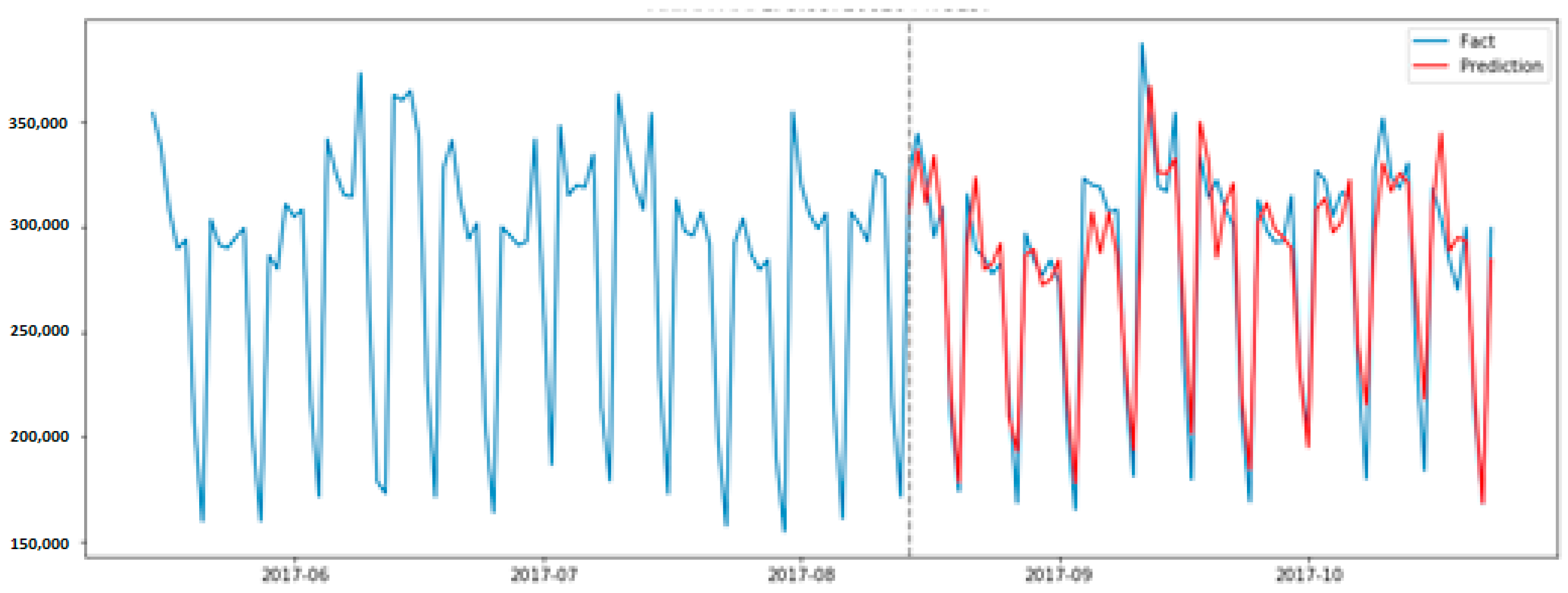
5.1. Case 1. Forecasting Demand in ATMs

Forecasting the demand for cash in ATMs is associated with their optimal loading. Optimal loading of cash should be carried out for two purposes. First, this amount should be minimal to avoid a sizeable unclaimed cash balance since the money must be circulated within the monetary system of the entire country. Secondly, the maximum should be the amount that meets customer demand and a guaranteed level of customer service quality, since insufficient funds lead to a negative customer experience. Also, the sudden use of all cash in ATMs leads to downtime, reducing the efficiency of using the ATM network and, consequently, the bank’s profit.

Using the MAPE metric, we determined that the average forecast error for a time series (a separate row for each ATM) is about 18% (Figure 3).

Figure 3. Comparison of actual and forecast values using a time series of demand for cash in one of the ATMs (blue—actual values; red—forecast).

The distribution of anomalies by days of the month for a given series is shown in Figure 4. Visualizations built using the SHAP library were used to display the influence of variables on decision-making using an algorithm in a business-friendly language (Baptista and Poloczek 2018). This method facilitated the display, in an accessible form, of the influence of variables on decision-making. At the same time, the decisive variables can be displayed in an accessible way for each device on a specific day.

Figure 4. Interpretation of a forecast on a May 1 holiday.

In order to demonstrate the applicability of the proposed method, several case studies were conducted.

On a holiday—1 May 2019 (Figure 4).

It can be seen that the following factors influenced the downward trend (blue color) of the forecast demand: no one withdraws cash, since it was already withdrawn on April 30) and decreased demand 4 and 6 days ago. The upward (red) trendwas increased demand on the pre-holiday day, April 30.

On the day of mass payments—10 July 2019 (Figure 5).

Figure 5. Interpretation of forecasts on the day of mass payments.

Based on the graph, it can be seen that the following factors influenced the increase in the forecast demand: the day of the week is Saturday, not a holiday, there was an increase in demand seven days ago, the indicator predicted this was a day of massive payments (abnormal demand).

5.2. Case 2. Forecasting the Load on Cash Centers

According to the MAPE metric, the average forecast error for this case for all series did not exceed 11% (Figure 6).

Figure 6. Actual and predicted values of the load level on the cash center.

It can be seen from the graph that the fact that May 1, 2019 is a holiday (the value of the is_holiday attribute = 1) played in the direction of decreasing (blue) the predicted load (Figure 7).

Figure 7. Interpretation of the forecast of the load on the CC on a holiday.

5.3. Case 3. Forecasting the Load on the Call Centers

For this case, the forecasting pipeline’s average error (according to the MAPE metric) did not exceed 8% across all call centers (Figure 8).

Figure 8. Visualization of the forecast of the load on the call center.

Thus, the development of predictive models of a non-stationary time series according to the above technique allows one to save labor costs for several weeks by automatically generating the feature space, selecting features, selecting the best model, and effectively selecting hyperparameters. The built-in detection of anomalies allows one to improve prediction quality on average by 10%, as measured by the MAPE metric, by identifying periodic anomalies and generating the corresponding signs (Table 3).

Table 3. Results of analyzed cases using the MAPE metric.

Case No.	MAPE Score with Anomaly Detection	MAPE Score without Anomaly Detection
1	18%	29%
2	11%	24%
3	8%	18%

6. Conclusions

The article developed a universal scenario for forecasting a non-stationary time series in automatic mode. The developed scenario for solving specific banking tasks to improve business efficiency, including optimizing demand in ATMs and forecasting the load on the call center and cash center, was considered.

New information technologies were used based on machine learning, based on the principle of training models based on available data on the operation of ATMs, to implement this task. As a result, a universal methodology and software was developed to automate the stages associated with the automatic generation of the feature space, anomaly detection, selection of hyperparameters, and training models.

Based on the above results, we can conclude that the approved methodology for constructing machine learning systems is fully applicable to creating predictive models in economics and finance. Looking back at the literature, we can confidently say that intelligent methods give a clearly expressed applied result in predictive economic and financial problems by significantly reducing the time cost of data research by automating the processes of identifying features.

Thus, we can discuss a stable and continuing trend for introducing intelligent methods in economics and finance. The results obtained in this study significantly reduce the overhead costs for servicing ATMs and carrying out cash collection due to the more accurate prediction of the moments of the required loading, and as a result improve overall logistics.

In this research, we studied the issues of forecasting a time series precisely, as it is one of the most common types of datasets in this area. By applying data mining and machine learning methods, this technique, with the necessary modifications, can be used for predictive or descriptive analysis and other data formats, but further research is needed for a more accurate conclusion.

As for directions for further research, we would like to note the following promising areas: the study of the stability and interpretability of the obtained solutions by more classical methods of mathematical statistics, the improvement of the machine learning methodology following the practice of MLOPS, the testing of the described methodology on other economic problems.

The proposed universal forecasting methodology can be built into the business model of a credit institution which is customer-focused, as it is associated with deep understanding and adequate customer satisfaction. Customer needs are met, in particular, by remote banking services (Internet banking, mobile banking), technologies for integrating banking services with other platforms and services, and the development of an ATM network.

References

1. Adeodato, Paulo, Adrian Arnaud, Germano Vasconcelos, Rodrigo Cunha, and Domingos Monteiro. 2014. NN5 Forecasting Competition-ADEODATO Paulo-CIn UFPE-BRAZIL. Available online: http://www.neural-forecasting-competition.com/NN5/ (accessed on 15 December 2021).
2. Aguilar-Rivera, Rubén, Manuel Valenzuela-Rendón, and J. J. Rodríguez-Ortiz. 2015. Genetic algorithms and Darwinian approaches in financial applications: A survey. Expert Systems with Applications 42: 7684–97. [Google Scholar] [CrossRef]
3. Aliev, Rafik Aziz, Bijan Fazlollahi, and Rashad Rafik Aliev. 2004. Soft Computing in Electronic Business. In Soft Computing and Its Applications in Business and Economics. Berlin/Heidelberg: Springer, pp. 431–46. [Google Scholar] [CrossRef]
4. Andrawis, Robert R., Amir F. Atiya, and Hisham El-Shishiny. 2011. Forecast combinations of computational intelligence and linear models for the NN5 time series forecasting competition. International Journal of Forecasting 27: 672–88. [Google Scholar] [CrossRef]
5. Arabani, Soodabeh Poorzaker, and Hosein Ebrahimpour Komleh. 2019. The Improvement of Forecasting ATMs Cash Demand of Iran Banking Network Using Convolutional Neural Network. Arabian Journal for Science and Engineering 44: 3733–43. [Google Scholar] [CrossRef]
6. Asad, Muhammad, Muhammad Shahzaib, Yusra Abbasi, and Muhammad Rafi. 2020. A Long-Short-Term-Memory Based Model for Predicting ATM Replenishment Amount. Paper present at the 2020 21st International Arab Conference on Information Technology (ACIT), Giza, Egypt, November 28–30. [Google Scholar] [CrossRef]
7. Atsalakis, George S., and Kimon P. Valavanis. 2009. Surveying stock market forecasting techniques—Part II: Soft computing methods. Expert Systems with Applications 36: 5932–41. [Google Scholar] [CrossRef]
8. Aue, Alexander, Lajos Horváth, Mario Kühn, and Josef Steinebach. 2012. On the reaction time of moving sum detectors. Journal of Statistical Planning and Inference 142: 2271–88. [Google Scholar] [CrossRef]
9. Bahrammirzaee, Arash. 2010. Comparative survey of artificial intelligence applications in finance: Artificial neural networks, expert system and hybrid intelligent systems. Neural Computing & Applications 19: 1165–95. [Google Scholar] [CrossRef]
10. Baptista, Ricardo, and Matthias Poloczek. 2018. Bayesian Optimization of Combinatorial Structures. International Conference on Machine Learning, Proceedings of Machine Learning Research. pp. 462–71. Available online: http://proceedings.mlr.press/v80/baptista18a.html (accessed on 15 December 2021).
11. Catal, Cagatay, Ayse Fenerci, Burcak Ozdemir, and Onur Gulmez. 2015. Improvement of Demand Forecasting Models with Special Days. Procedia Computer Science 59: 262–67. [Google Scholar] [CrossRef] [Green Version]
12. Cavalcante, Rodolfo C., Rodrigo C. Brasileiro, Victor LF Souza, Jarley P. Nobrega, and Adriano LI Oliveira. 2016. Computational Intelligence and Financial Markets: A Survey and Future Directions. Expert Systems with Applications 55: 194–211. [Google Scholar] [CrossRef]
13. Cerqueira, Vitor, Luis Torgo, and Igor Mozetič. 2020. Evaluating time series forecasting models: An empirical study on performance estimation methods. Machine Learning 109: 1997–2028. [Google Scholar] [CrossRef]
14. Chatterjee, Amitava, O. Felix Ayadi, and Bryan E. Boone. 2000. Artificial Neural Network and the Financial Markets: A Survey. Managerial Finance 26: 32–45. [Google Scholar] [CrossRef]
15. Chen, Shu-Heng. 2002. Genetic Algorithms and Genetic Programming in Computational Finance: An Overview of the Book. In Genetic Algorithms and Genetic Programming in Computational Finance. Boston: Springer, pp. 1–26. [Google Scholar] [CrossRef]
16. Claesen, Marc, and Bart De Moor. 2015. Hyperparameter Search in Machine Learning. arXiv arXiv:1502.02127. [Google Scholar]
17. Das, Abhimanyu, and David Kempe. 2011. Submodular meets Spectral: Greedy Algorithms for Subset Selection, Sparse Approximation and Dictionary Selection. arXiv arXiv:1102.3975. [Google Scholar]
18. Draper, Norman R., and Harry Smith. 1998. Applied Regression Analysis. Wiley Series in Probability and Statistics; New York: Wiley. [Google Scholar] [CrossRef]
19. Dymowa, Ludmila. 2011. Soft Computing in Economics and Finance. Intelligent Systems Reference Library. Berlin/Heidelberg: Springer. [Google Scholar] [CrossRef]
20. Ekinci, Yeliz, Jye-Chyi Lu, and Ekrem Duman. 2015. Optimization of ATM cash replenishment with group-demand forecasts. Expert Systems with Applications 42: 3480–90. [Google Scholar] [CrossRef]
21. Ekinci, Yeliz, Nicoleta Serban, and Ekrem Duman. 2019. Optimal ATM replenishment policies under demand uncertainty. Operational Research 21: 999–1029. [Google Scholar] [CrossRef]
22. Elmsili, B., and B. Outtaj. 2018. Artificial neural networks applications in economics and management research: An exploratory literature review. Paper present at the 4th International Conference on Optimization and Applications (ICOA), ENSET of Mohammedia, BP 159, BD Hassan II, Mohammedia, Morocco, April 26–27. [Google Scholar] [CrossRef]
23. Fremdt, Stefan. 2015. Page’s sequential procedure for change-point detection in time series regression. Statistics 49: 128–55. [Google Scholar] [CrossRef] [Green Version]
24. Hasheminejad, Seyed Mohammad Hossein, and Zahra Reisjafari. 2017. ATM management prediction using Artificial Intelligence techniques: A survey. Intelligent Decision Technologies 11: 375–98. [Google Scholar] [CrossRef]
25. Hewamalage, Hansika, Christoph Bergmeir, and Kasun Bandara. 2021. Recurrent Neural Networks for Time Series Forecasting: Current status and future directions. International Journal of Forecasting 37: 388–427. [Google Scholar] [CrossRef]
26. Hu, Yong, Kang Liu, Xiangzhou Zhang, Lijun Su, E. W. T. Ngai, and Mei Liu. 2015. Application of evolutionary computation for rule discovery in stock algorithmic trading: A literature review. Applied Soft Computing 36: 534–51. [Google Scholar] [CrossRef]
27. Jadwal, Pankaj Kumar, Sonal Jain, Umesh Gupta, and Prashant Khanna. 2018. K-Means Clustering with Neural Networks for ATM Cash Repository Prediction. Paper present at the Information and Communication Technology for Intelligent Systems (ICTIS 2017), Ahmedabad, India, March 25–26; vol. 1, pp. 588–96. [Google Scholar] [CrossRef]
28. Kamini, Venkatesh, Vadlamani Ravi, and D. Nagesh Kumar. 2014. Chaotic time series analysis with neural networks to forecast cash demand in ATMs. Paper present at the 2014 IEEE International Conference on Computational Intelligence and Computing Research, Coimbatore, India, December 18–20. [Google Scholar] [CrossRef]
29. Katarya, Rahul, and Anmol Mahajan. 2017. A survey of neural network techniques in market trend analysis. Paper present at the 2017 International Conference on Intelligent Sustainable Systems (ICISS), Tirupur, India, December 7–8. [Google Scholar] [CrossRef]
30. Khanarsa, Paisit, and Krung Sinapiromsaran. 2017. Multiple ARIMA subsequences aggregate time series model to forecast cash in ATM. Paper present at the 2017 9th International Conference on Knowledge and Smart Technology (KST), Wolfenbüttel, Germany, February 1–4. [Google Scholar] [CrossRef]
31. Kovalerchuk, Boris, and Evgenii Vityaev. 2006. Data Mining in Finance: Advances in Relational and Hybrid Methods. Berlin/Heidelberg: Springer Science & Business Media, Available online: https://play.google.com/store/books/details?id=quDlBwAAQBAJ (accessed on 15 December 2021).
32. Li, Yuhong, and Weihua Ma. 2010. Applications of Artificial Neural Networks in Financial Economics: A Survey. Paper present at the 2010 International Symposium on Computational Intelligence and Design, Hangzhou, China, October 29–31. [Google Scholar] [CrossRef]
33. Lundberg, Scott M., and Su-In Lee. 2017. A Unified Approach to Interpreting Model Predictions. arXiv arXiv:1705.07874. [Google Scholar]
34. Morariu, Nicolae, Eugenia Iancu, and Sorin Vlad. 2009. A Neural Network Model for Time-Series Forecasting. Journal for Economic Forecasting 4: 213–23. Available online: https://ipe.ro/rjef/rjef4_09/rjef4_09_13.pdf (accessed on 15 December 2021).
35. Nair, Binoy B., and V. P. Mohandas. 2014. Artificial intelligence applications in financial forecasting—A survey and some empirical results. Intelligent Decision Technologies 9: 99–140. [Google Scholar] [CrossRef]
36. Ozer, Fazilet, Ismail Hakki Toroslu, Pinar Karagoz, and Ferhat Yucel. 2019. Dynamic Programming Solution to ATM Cash Replenishment Optimization Problem. In International Conference on Intelligent Computing & Optimization. Cham: Springer, pp. 428–37. [Google Scholar] [CrossRef]
37. Ponsich, Antonin, Antonio Lopez Jaimes, and Carlos A. Coello Coello. 2013. A Survey on Multiobjective Evolutionary Algorithms for the Solution of the Portfolio Optimization Problem and Other Finance and Economics Applications. IEEE Transactions on Evolutionary Computation 17: 321–44. [Google Scholar] [CrossRef]
38. Pradeepkumar, Dadabada, and Vadlamani Ravi. 2018. Soft computing hybrids for FOREX rate prediction: A comprehensive review. Computers & Operations Research 99: 262–84. [Google Scholar] [CrossRef]
39. Rafi, Muhammad, Mohammad Taha Wahab, Muhammad Bilal Khan, and Hani Raza. 2020. ATM Cash Prediction Using Time Series Approach. Paper present at the 2020 3rd International Conference on Computing, Mathematics and Engineering Technologies (iCoMET), Sindh, Pakistan, January 29–30. [Google Scholar] [CrossRef]
40. Rajwani, Akber, Tahir Syed, Behraj Khan, and Sadaf Behlim. Regression Analysis for ATM Cash Flow Prediction. Paper present at the International Conference on Frontiers of Information Technology (FIT), Islamabad, Pakistan, December 18–20. [CrossRef]
41. Rong, Jingfeng, and Di Wang. 2021. Research on Prediction of the Cash Usage in Banks Based on LSTM of Improved Gray Wolf Optimizer. Journal of Physics: Conference Series 1769: 012031. [Google Scholar] [CrossRef]
42. Serengil, Sefik Ilkin, and Alper Ozpinar. 2019. ATM Cash Flow Prediction and Replenishment Optimization with ANN. Uluslararası Muhendislik Arastirma ve Gelistirme Dergisi 11: 402–8. [Google Scholar] [CrossRef]
43. Sezer, Omer Berat, Mehmet Ugur Gudelek, and Ahmet Murat Ozbayoglu. 2020. Financial time series forecasting with deep learning: A systematic literature review: 2005–2019. Applied Soft Computing 90: 106181. [Google Scholar] [CrossRef] [Green Version]
44. Shcherbitsky, V. V., A. A. Panachev, M. A. Medvedeva, and E. I. Kazakova. 2019. On the prediction of dispenser status in ATM using gradient boosting method. AIP Conference Proceedings 2186: 050015. [Google Scholar] [CrossRef]
45. Slack, Dylan, Sophie Hilgard, Emily Jia, Sameer Singh, and Himabindu Lakkaraju. 2020. Fooling LIME and SHAP. Paper present at the AAAI/ACM Conference on AI, Ethics, and Society, New York, NY, USA, May 19. [Google Scholar] [CrossRef]
46. Tapia, Ma Guadalupe Castillo, and Carlos A. Coello Coello. 2007. Applications of multi-objective evolutionary algorithms in economics and finance: A survey. Paper present at the 2007 IEEE Congress on Evolutionary Computation, Singapore, September 25–28. [Google Scholar] [CrossRef]
47. Tkáč, Michal, and Robert Verner. 2016. Artificial neural networks in business: Two decades of research. Applied Soft Computing 38: 788–804. [Google Scholar] [CrossRef]
48. Vangala, Sarveswararao, and Ravi Vadlamani. 2020. ATM Cash Demand Forecasting in an Indian Bank with Chaos and Deep Learning. arXiv arXiv:2008.10365. [Google Scholar]
49. Venkatesh, Kamini, Vadlamani Ravi, Anita Prinzie, and Dirk Van den Poel. 2014. Cash demand forecasting in ATMs by clustering and neural networks. European Journal of Operational Research 232: 383–92. [Google Scholar] [CrossRef]
50. Yohannes, Yisehac, and Patrick Webb. 1999. Classification and Regression Trees, CART: A User Manual for Identifying Indicators of Vulnerability to Famine and Chronic Food Insecurity. Washington, DC: International Food Policy Research Institute, Available online: https://play.google.com/store/books/details?id=7iuq4ikyNdoC (accessed on 15 December 2021).
Publisher’s Note: MDPI stays neutral with regard to jurisdictional claims in published maps and institutional affiliations.
Article Metrics
Citations
Article Access Statistics
Multiple requests from the same IP address are counted as one view.