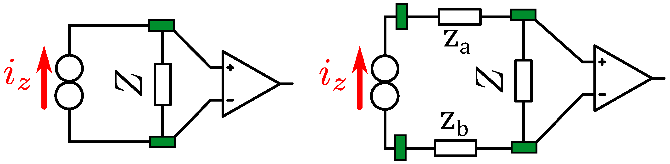
Figure 1.
Brief schematic of a bipolar measurement setup (
left) and a tetrapolar measurement setup (
right): green rectangles indicate the electrodes placed.
Z refers to the impedance under measure, while
and
refer to the bio-impedances between injection and measurement electrodes. The schematics are based on the description in [
11], assuming infinite current source output impedance, infinite instrumentation amplifier input impedance, and negligible electrode impedances.
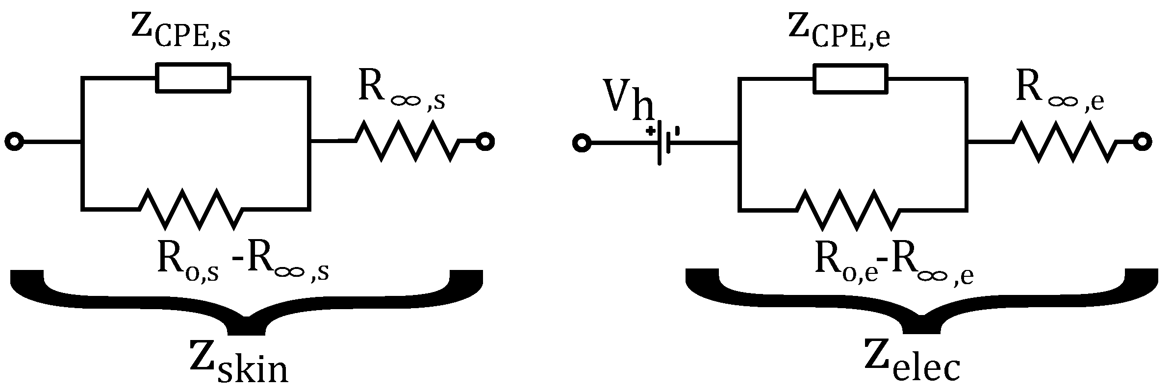
Figure 2.
Cole models of the skin (left) and electrode (right).
Figure 2.
Cole models of the skin (left) and electrode (right).
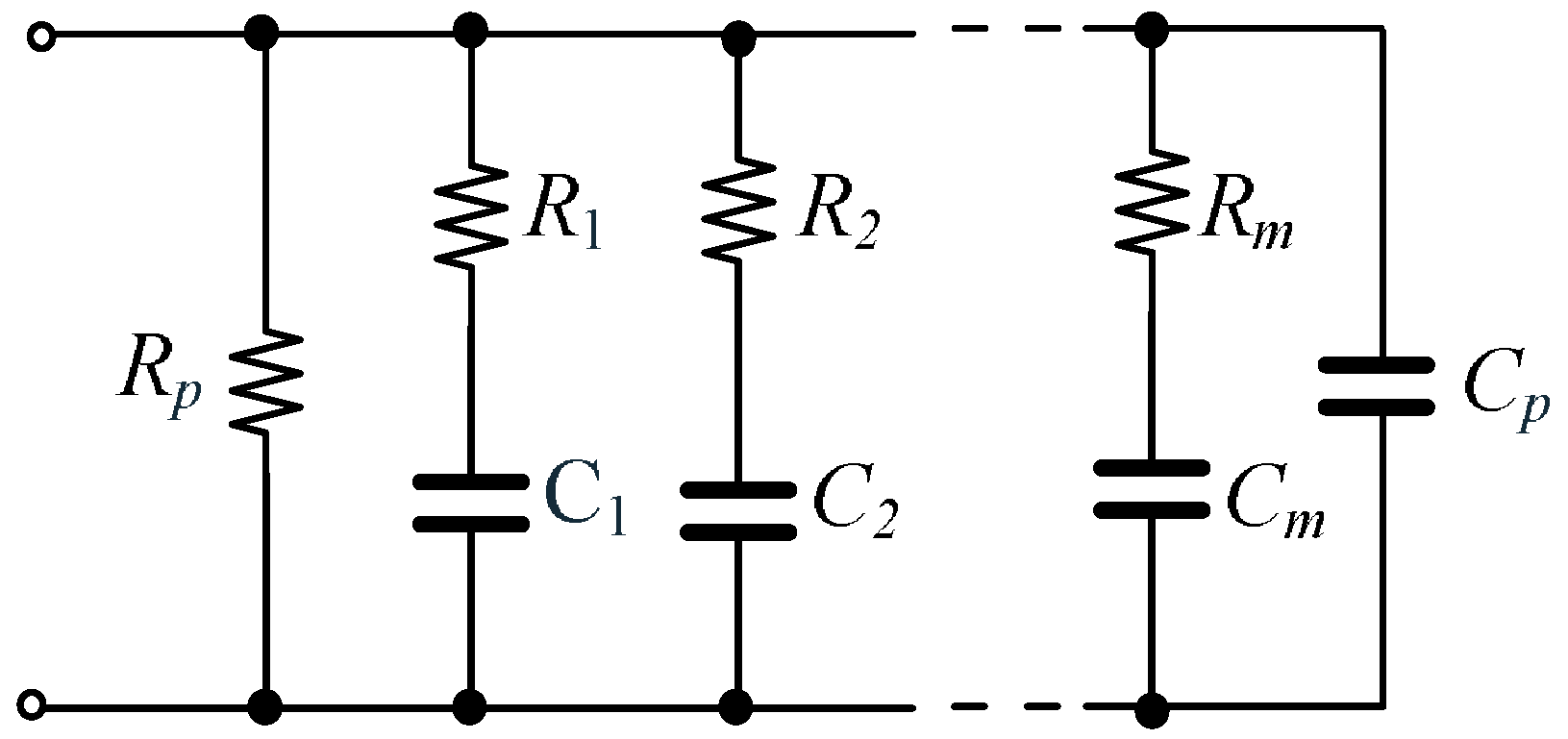
Figure 3.
RC network for approximating the behavior of fractional-order capacitors (
2) [
47].
Figure 3.
RC network for approximating the behavior of fractional-order capacitors (
2) [
47].
Figure 4.
Fractional-order capacitor emulator (versatile methodology) [
37].
Figure 4.
Fractional-order capacitor emulator (versatile methodology) [
37].
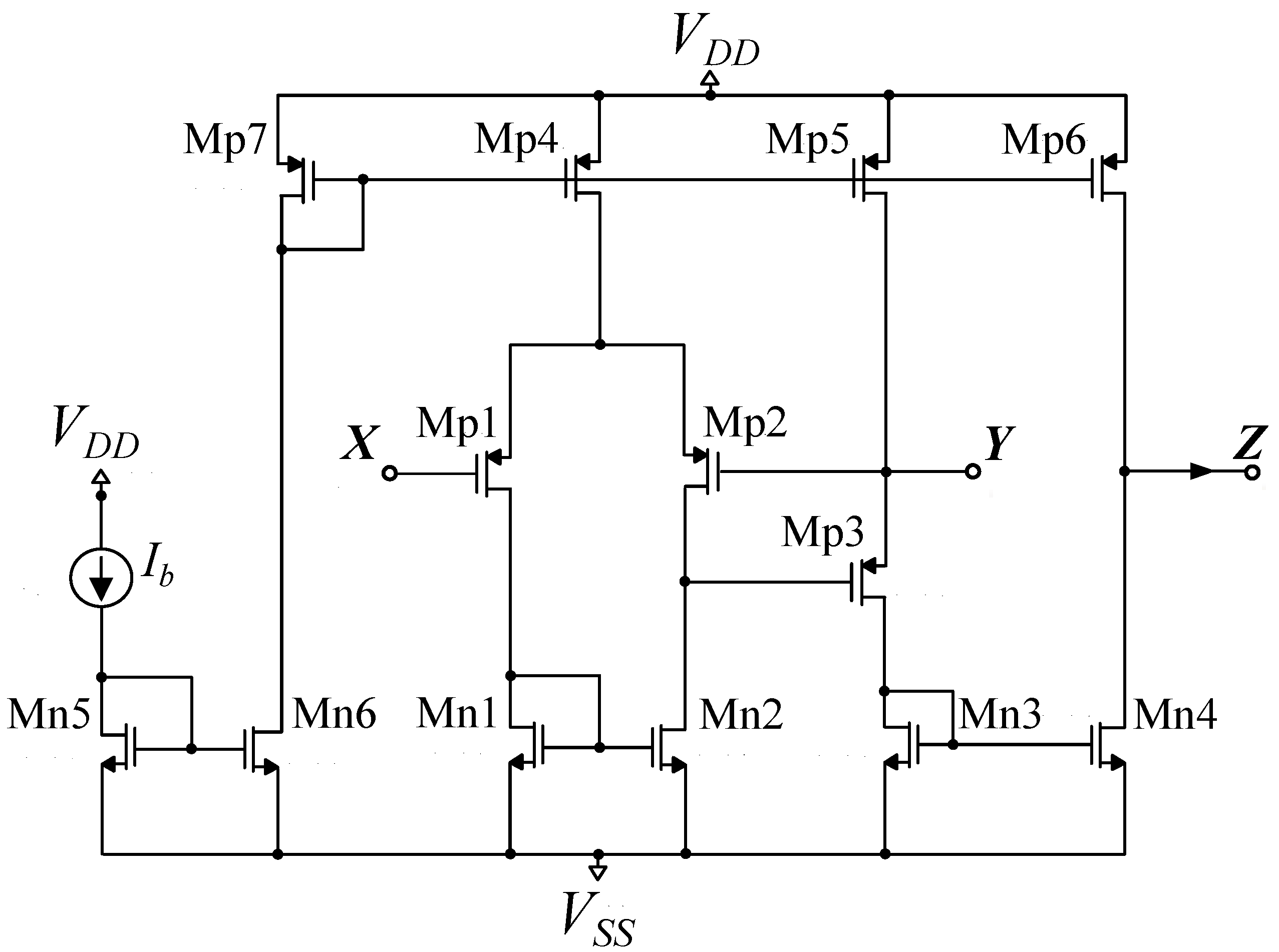
Figure 5.
Employed CCII [
37].
Figure 5.
Employed CCII [
37].
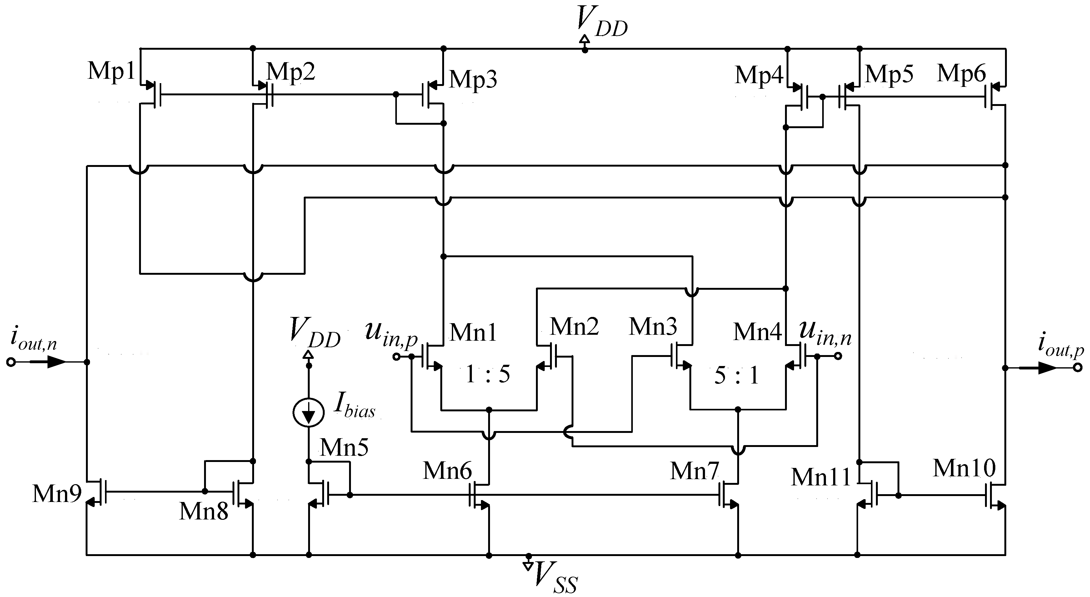
Figure 6.
Employed operational transconductance amplifier (OTA) [
37,
45].
Figure 6.
Employed operational transconductance amplifier (OTA) [
37,
45].
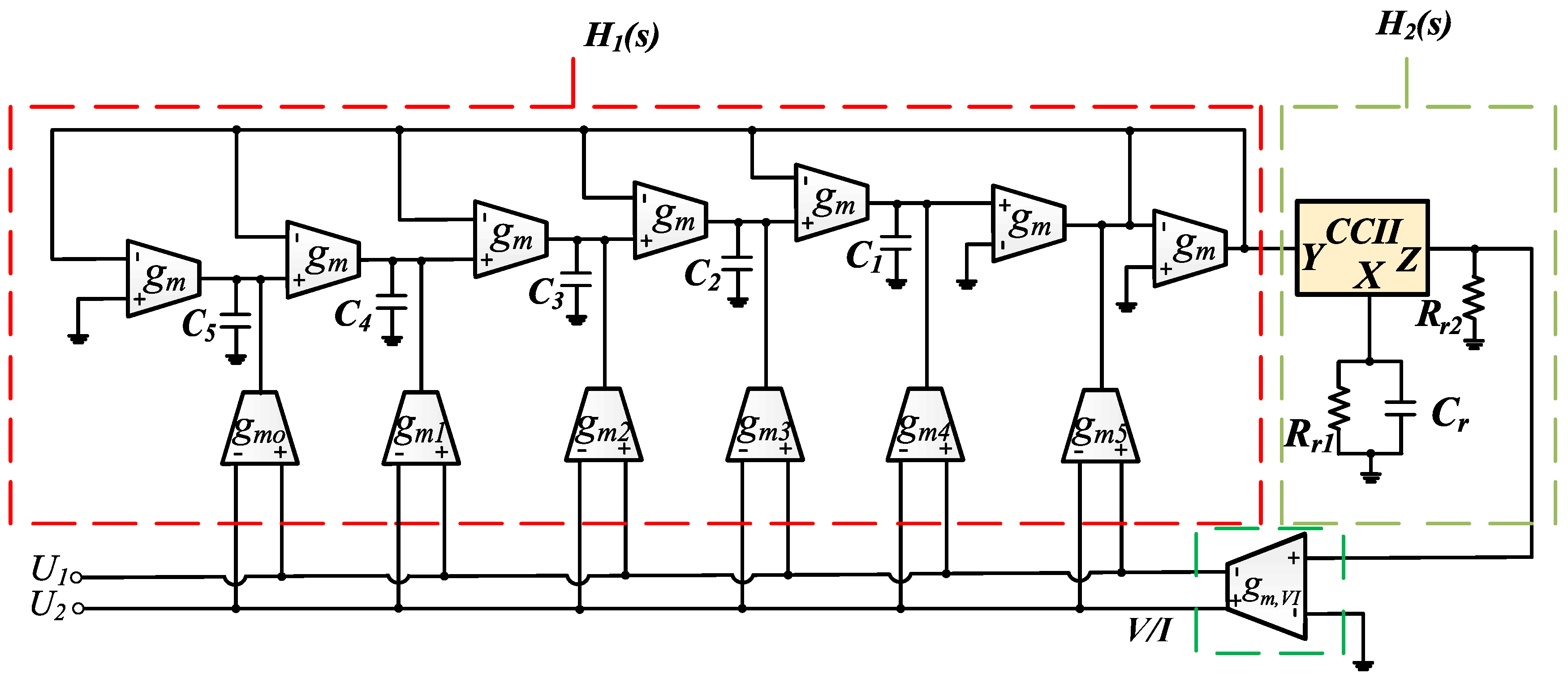
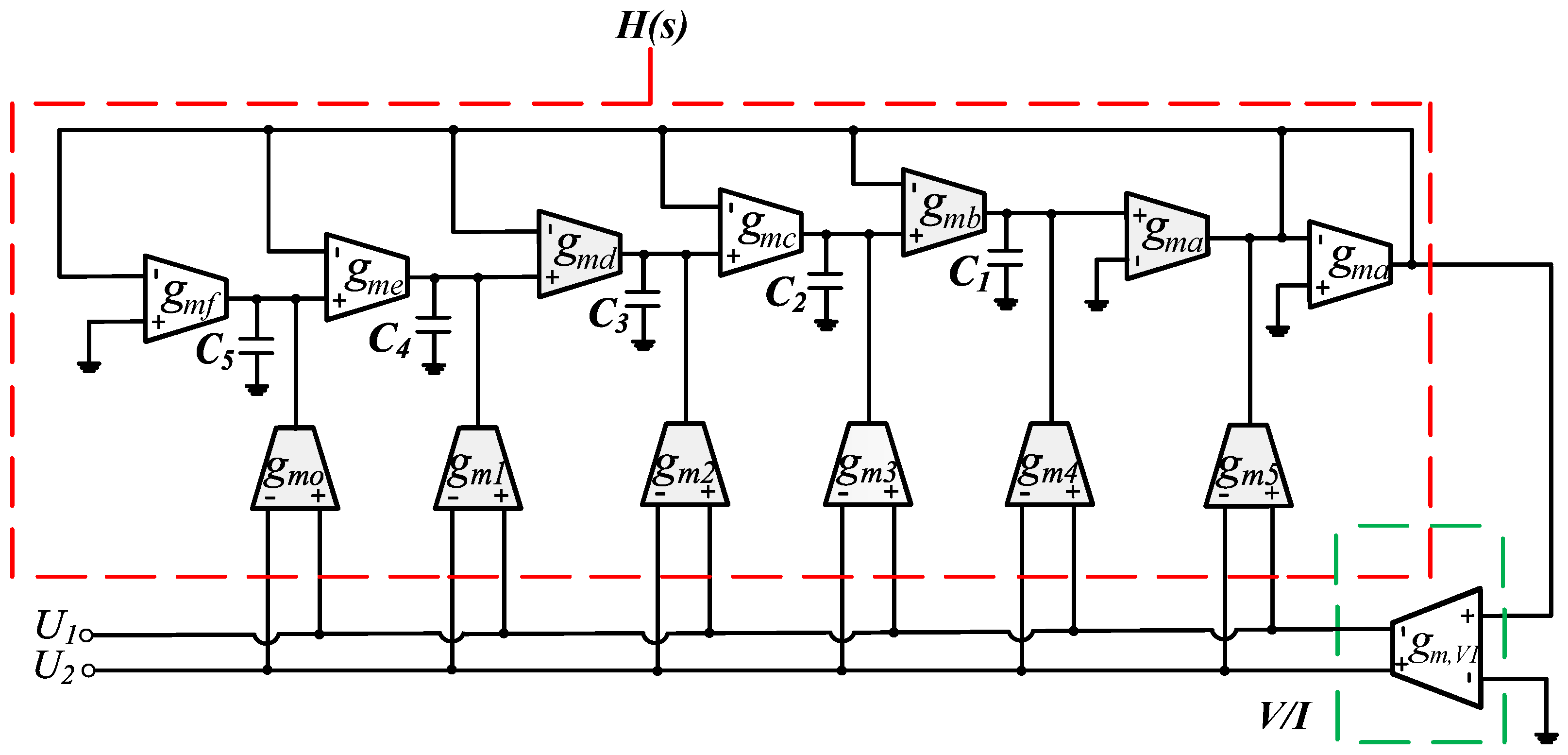
Figure 7.
Realization of fractional-order capacitor emulator (Inverse Follow-the-Leader Feedback (IFLF) methodology).
Figure 7.
Realization of fractional-order capacitor emulator (Inverse Follow-the-Leader Feedback (IFLF) methodology).
Figure 8.
Implementation of tunable resistor emulator [
37,
45].
Figure 8.
Implementation of tunable resistor emulator [
37,
45].
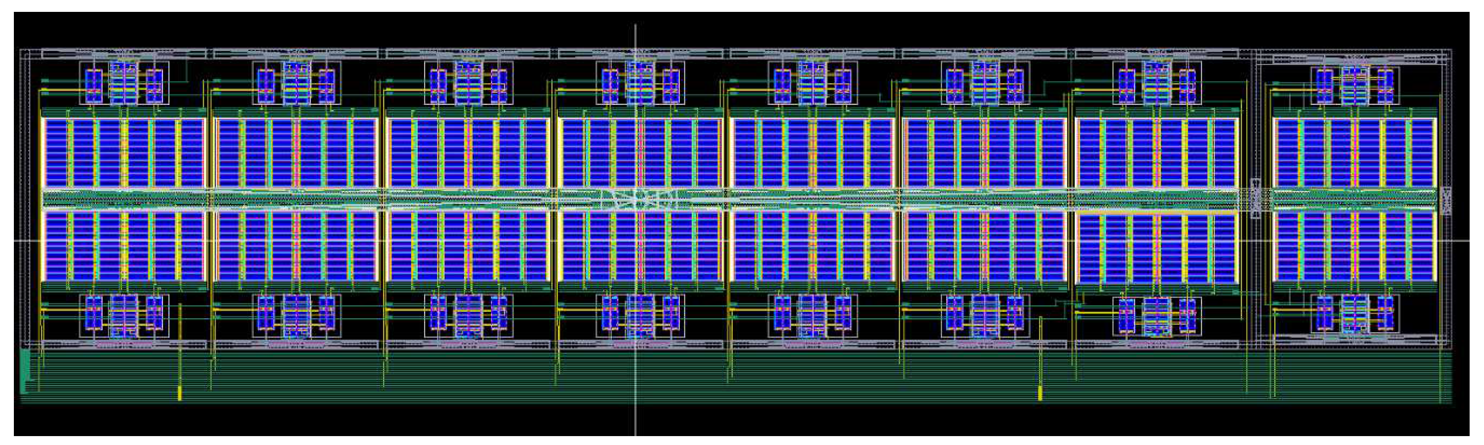
Figure 9.
Layout of the implemented fractional-order skin and electrode models (IFLF methodology).
Figure 9.
Layout of the implemented fractional-order skin and electrode models (IFLF methodology).
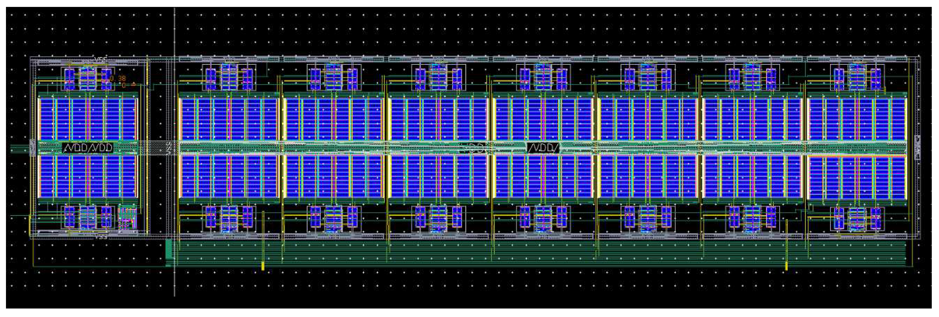
Figure 10.
Layout of the implemented fractional-order skin and electrode models (versatile methodology).
Figure 10.
Layout of the implemented fractional-order skin and electrode models (versatile methodology).
Figure 11.
Impedance magnitude (left) and phase response (right) of the fractional-order capacitor for the case of electrode model.
Figure 11.
Impedance magnitude (left) and phase response (right) of the fractional-order capacitor for the case of electrode model.
Figure 12.
Impedance magnitude (left) and phase response (right) of the fractional-order capacitor for the case of skin model.
Figure 12.
Impedance magnitude (left) and phase response (right) of the fractional-order capacitor for the case of skin model.
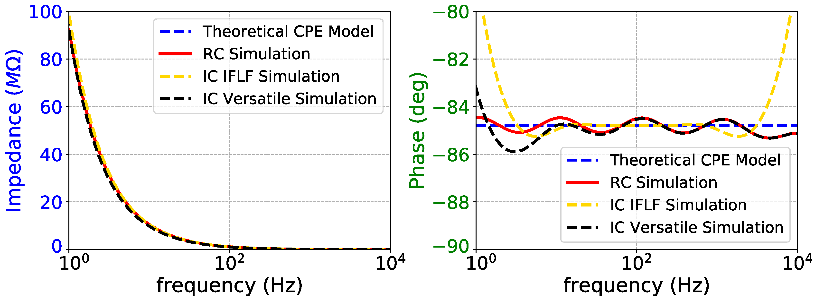
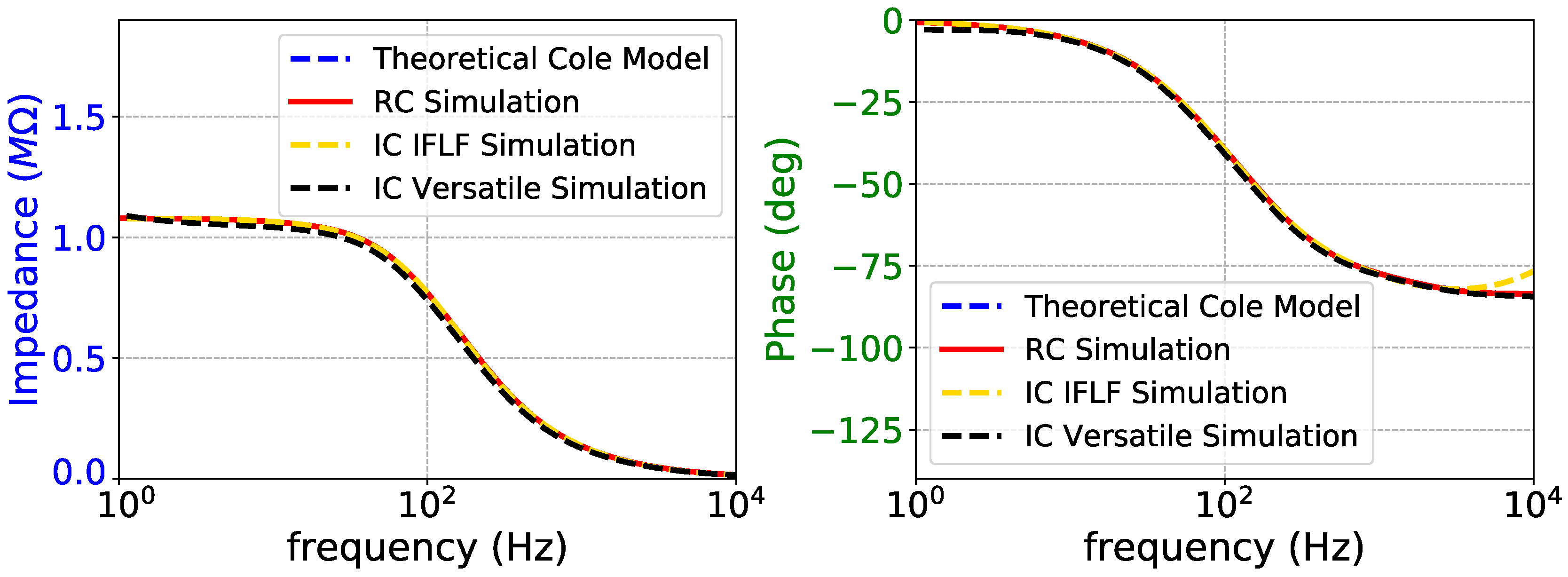
Figure 13.
Impedance magnitude (left) and phase response (right) of fractional-order electrode model.
Figure 13.
Impedance magnitude (left) and phase response (right) of fractional-order electrode model.
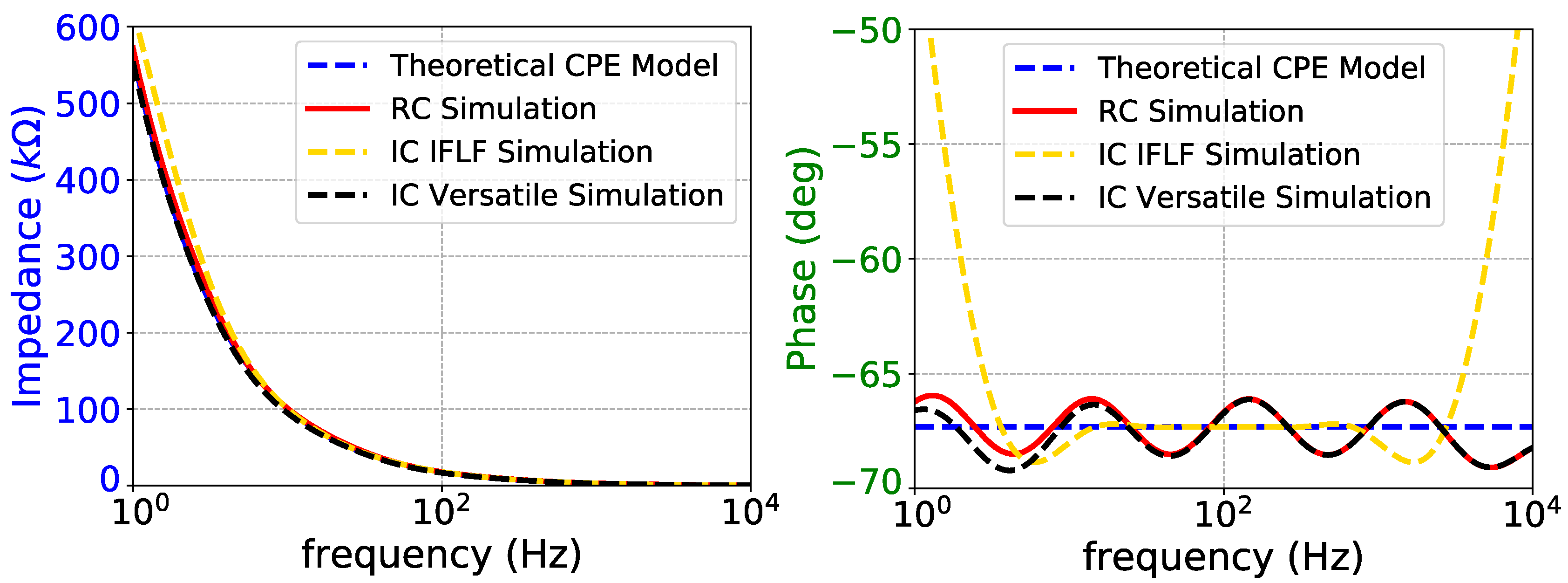
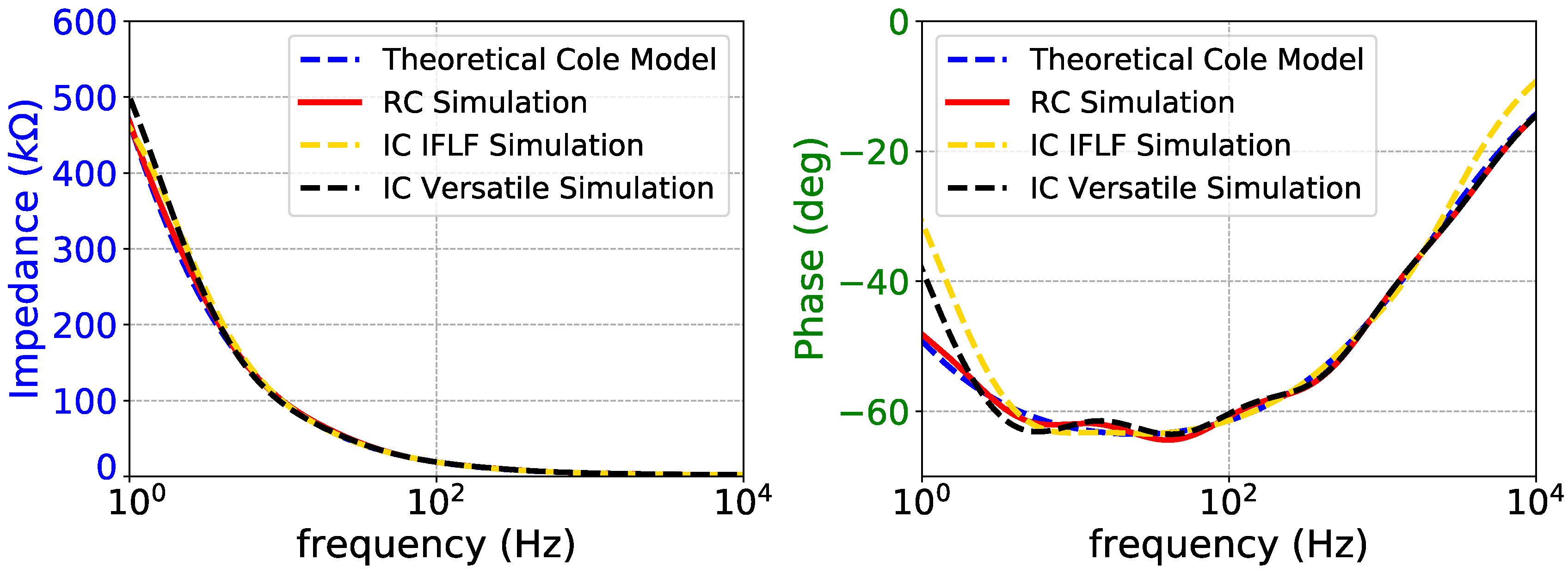
Figure 14.
Impedance magnitude (left) and phase response (right) of fractional-order skin model.
Figure 14.
Impedance magnitude (left) and phase response (right) of fractional-order skin model.
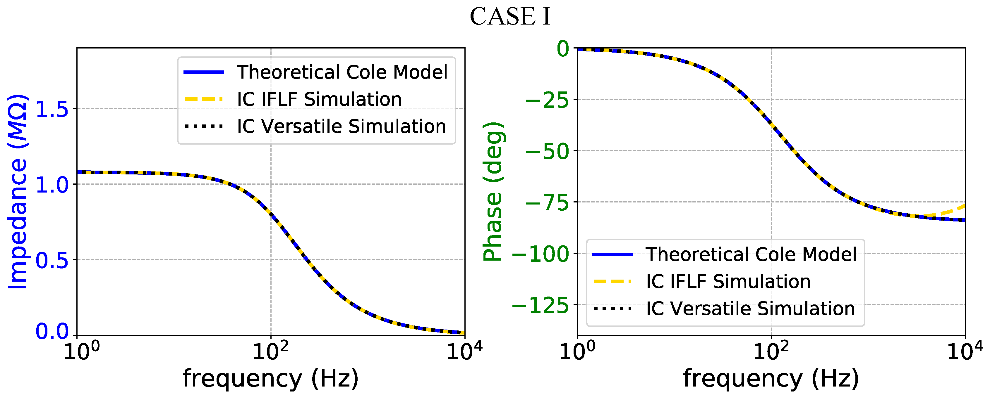
Figure 15.
Impedance magnitude (left) and phase response (right) of the case I fractional-order electrode model.
Figure 15.
Impedance magnitude (left) and phase response (right) of the case I fractional-order electrode model.
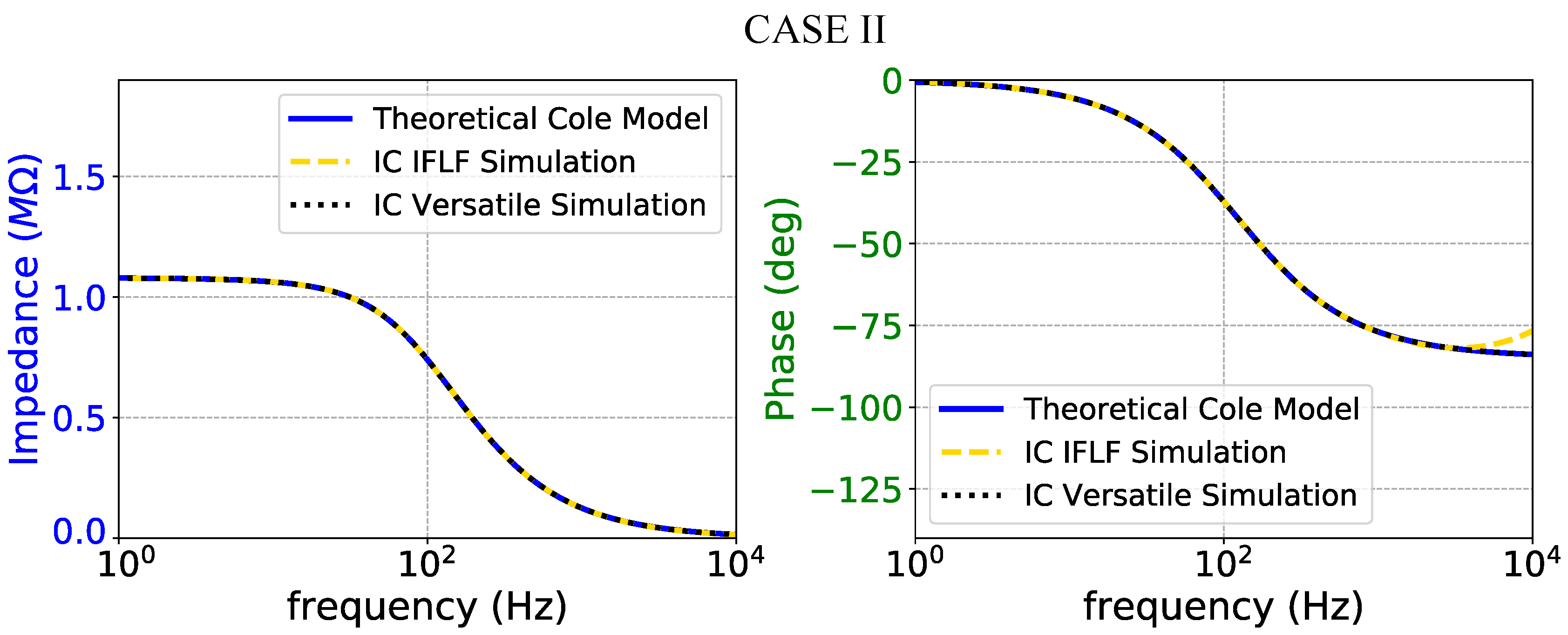
Figure 16.
Impedance magnitude (left) and phase response (right) of the case II fractional-order electrode model.
Figure 16.
Impedance magnitude (left) and phase response (right) of the case II fractional-order electrode model.
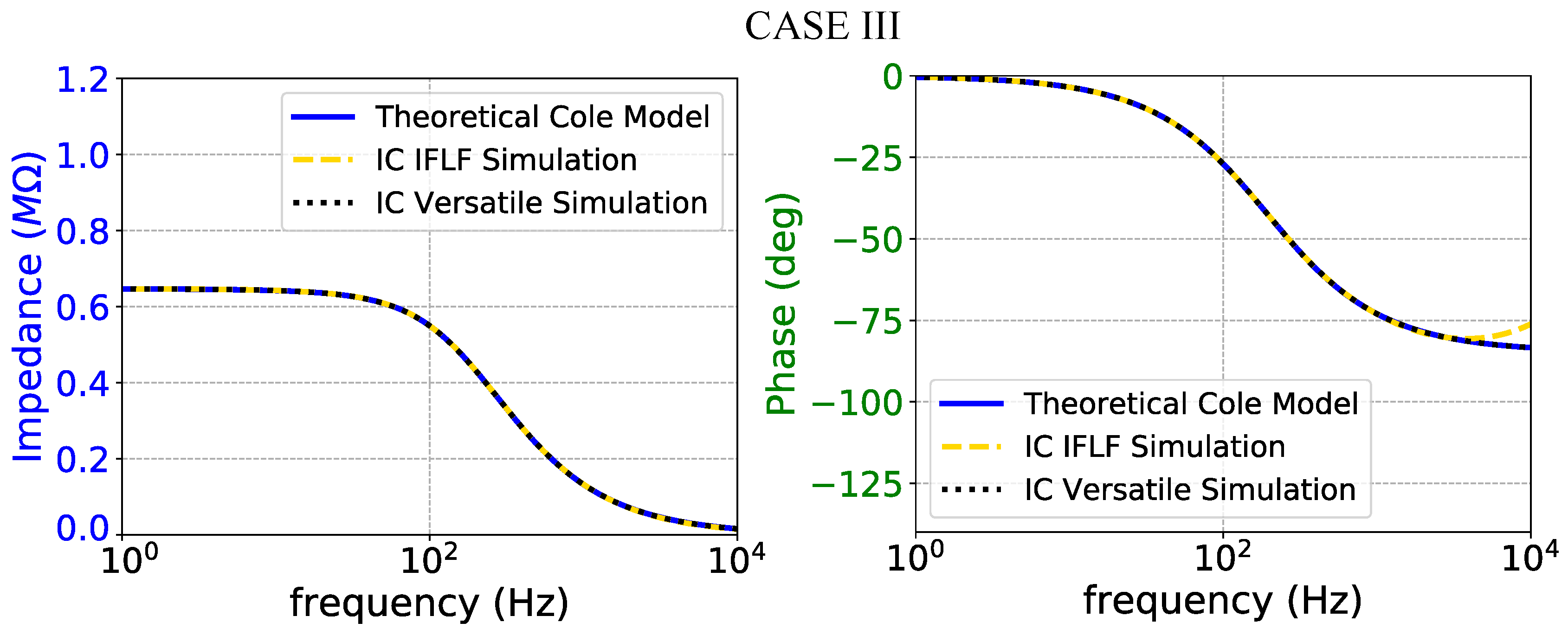
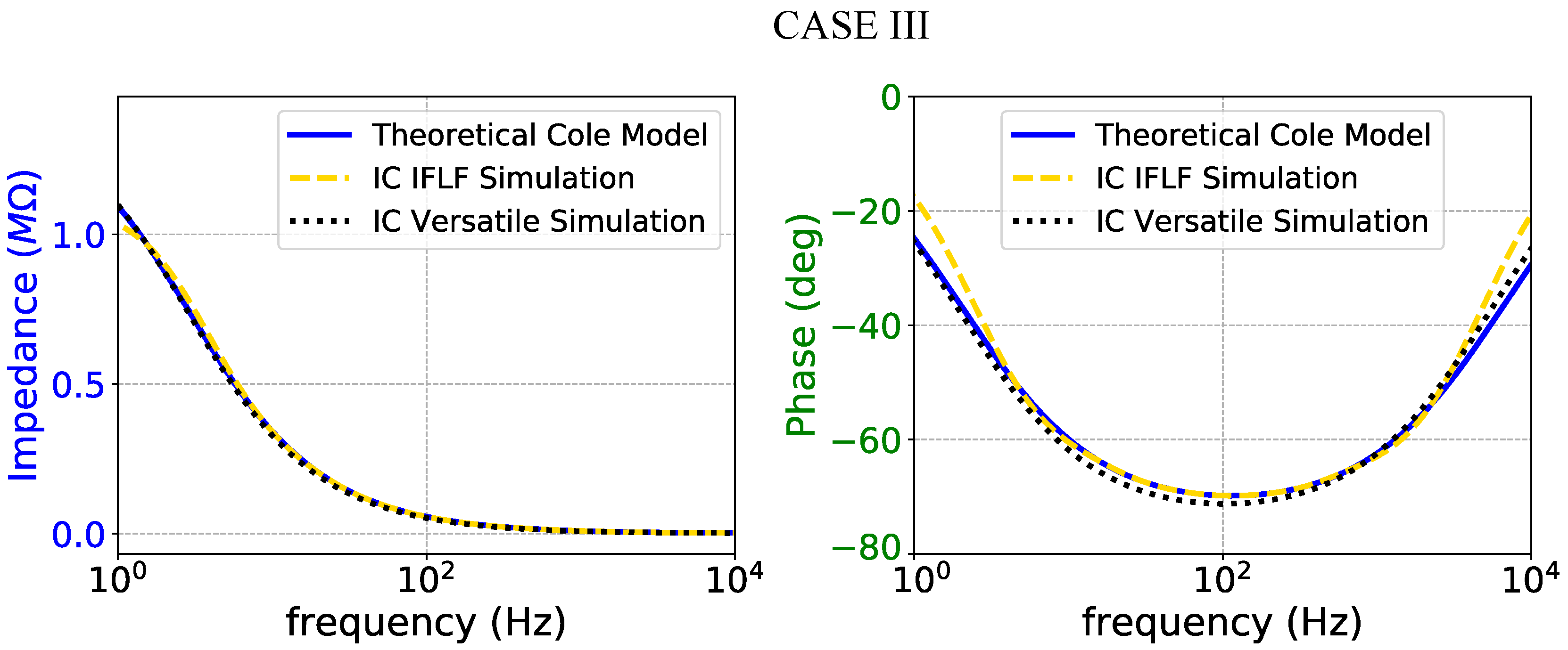
Figure 17.
Impedance magnitude (left) and phase response (right) of the case III fractional-order electrode model.
Figure 17.
Impedance magnitude (left) and phase response (right) of the case III fractional-order electrode model.
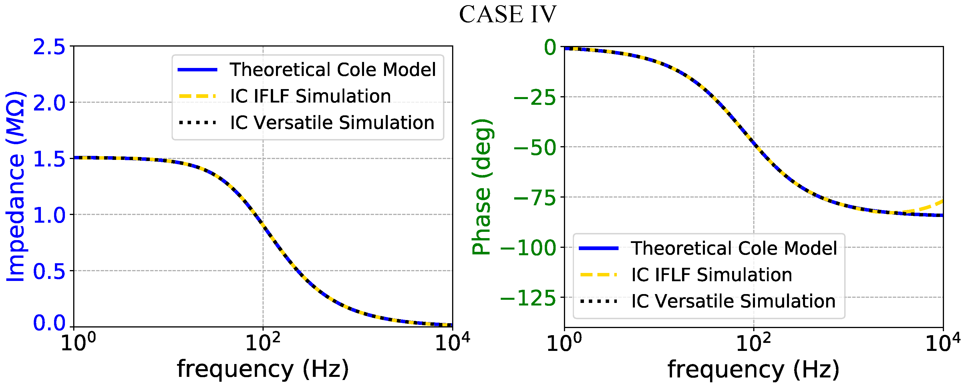
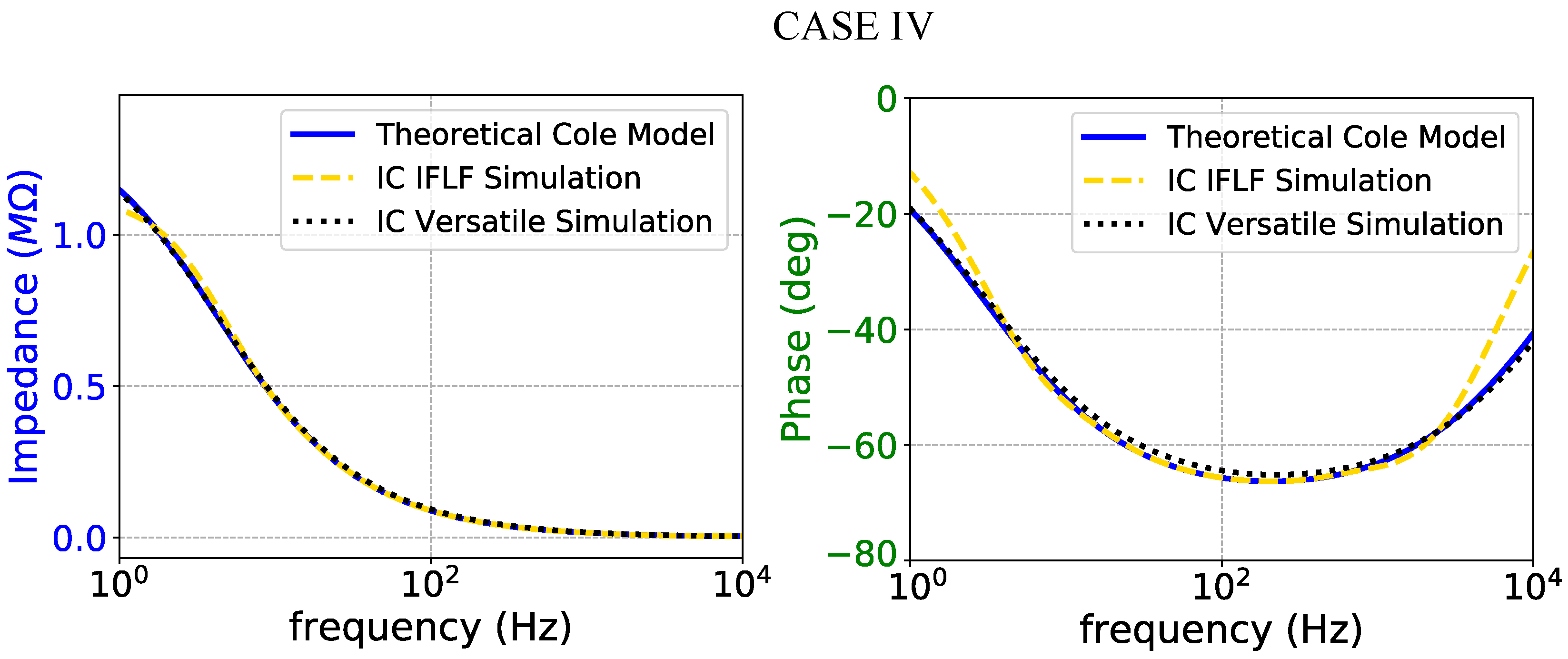
Figure 18.
Impedance magnitude (left) and phase response (right) of the case IV fractional-order electrode model.
Figure 18.
Impedance magnitude (left) and phase response (right) of the case IV fractional-order electrode model.
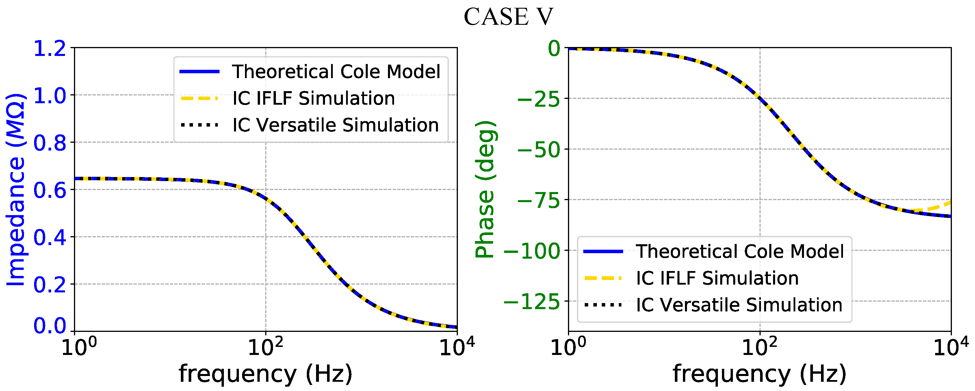
Figure 19.
Impedance magnitude (left) and phase response (right) of the case V fractional-order electrode model.
Figure 19.
Impedance magnitude (left) and phase response (right) of the case V fractional-order electrode model.
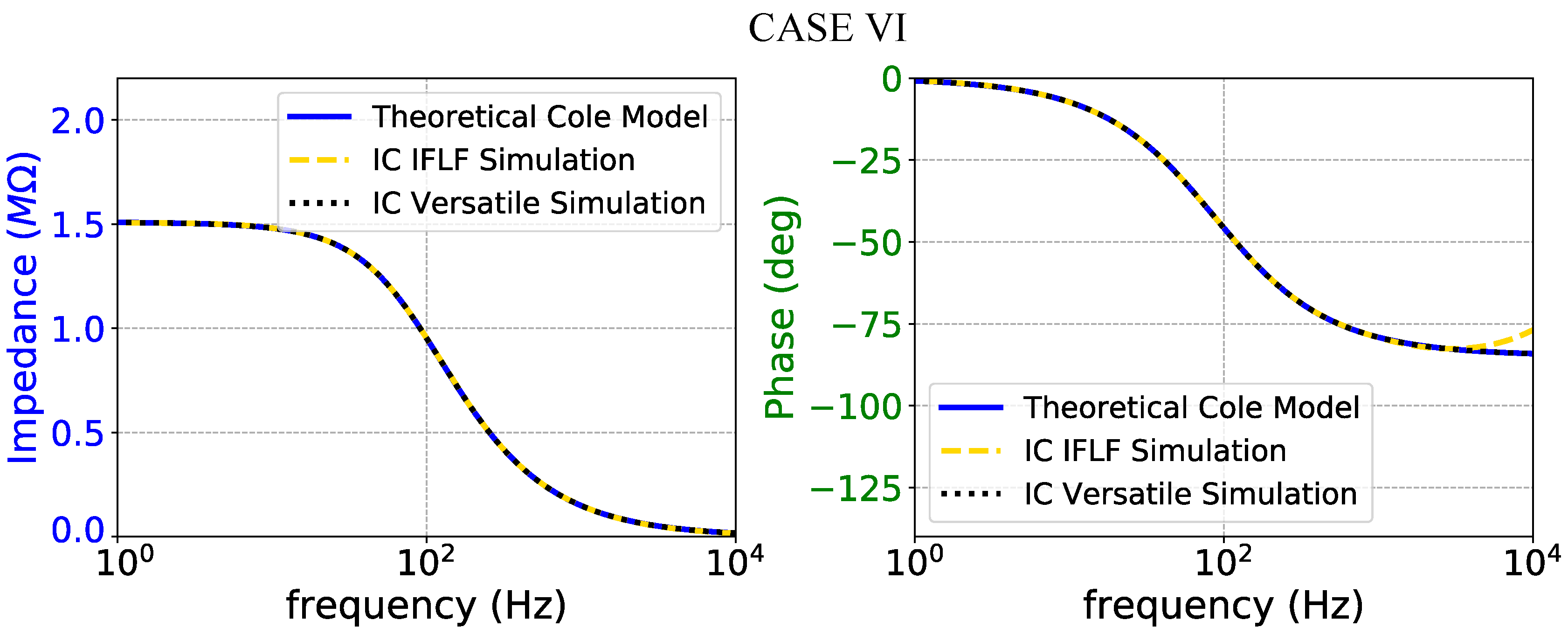
Figure 20.
Impedance magnitude (left) and phase response (right) of the case VI fractional-order electrode model.
Figure 20.
Impedance magnitude (left) and phase response (right) of the case VI fractional-order electrode model.
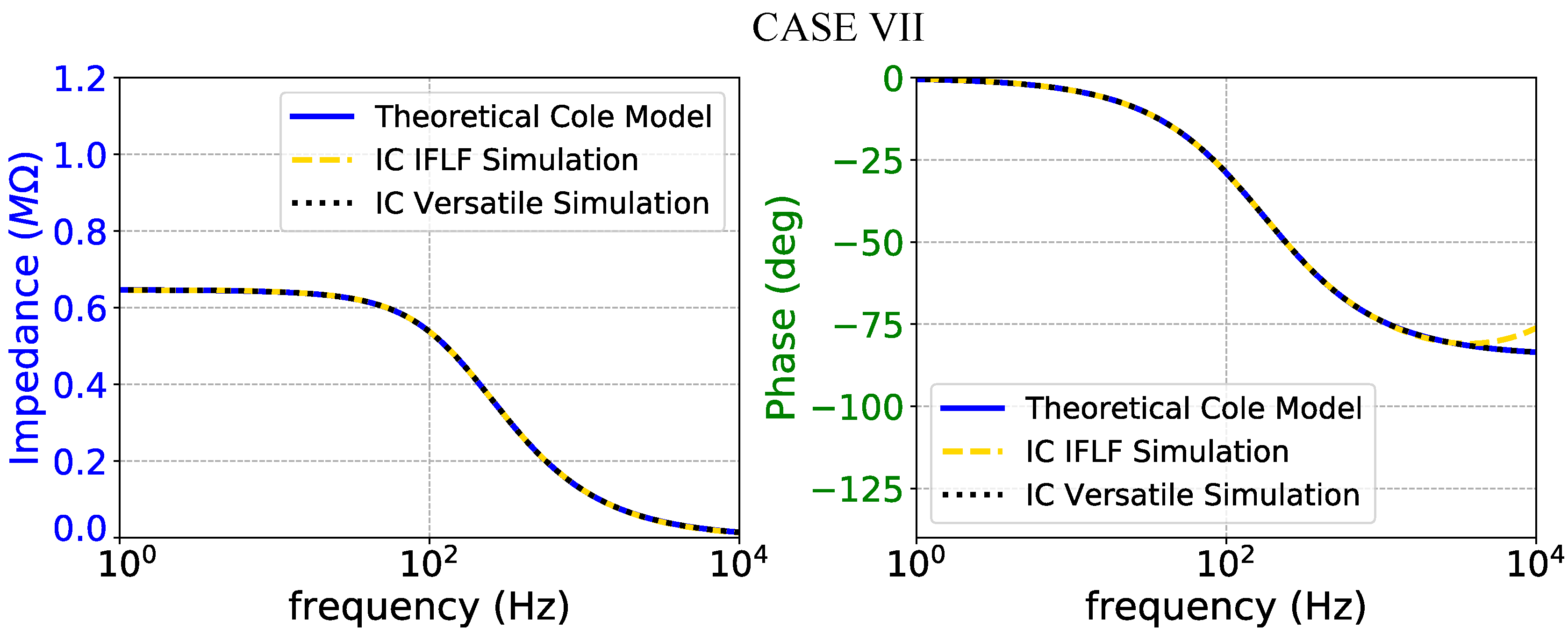
Figure 21.
Impedance magnitude (left) and phase response (right) of the case VII fractional-order electrode model.
Figure 21.
Impedance magnitude (left) and phase response (right) of the case VII fractional-order electrode model.
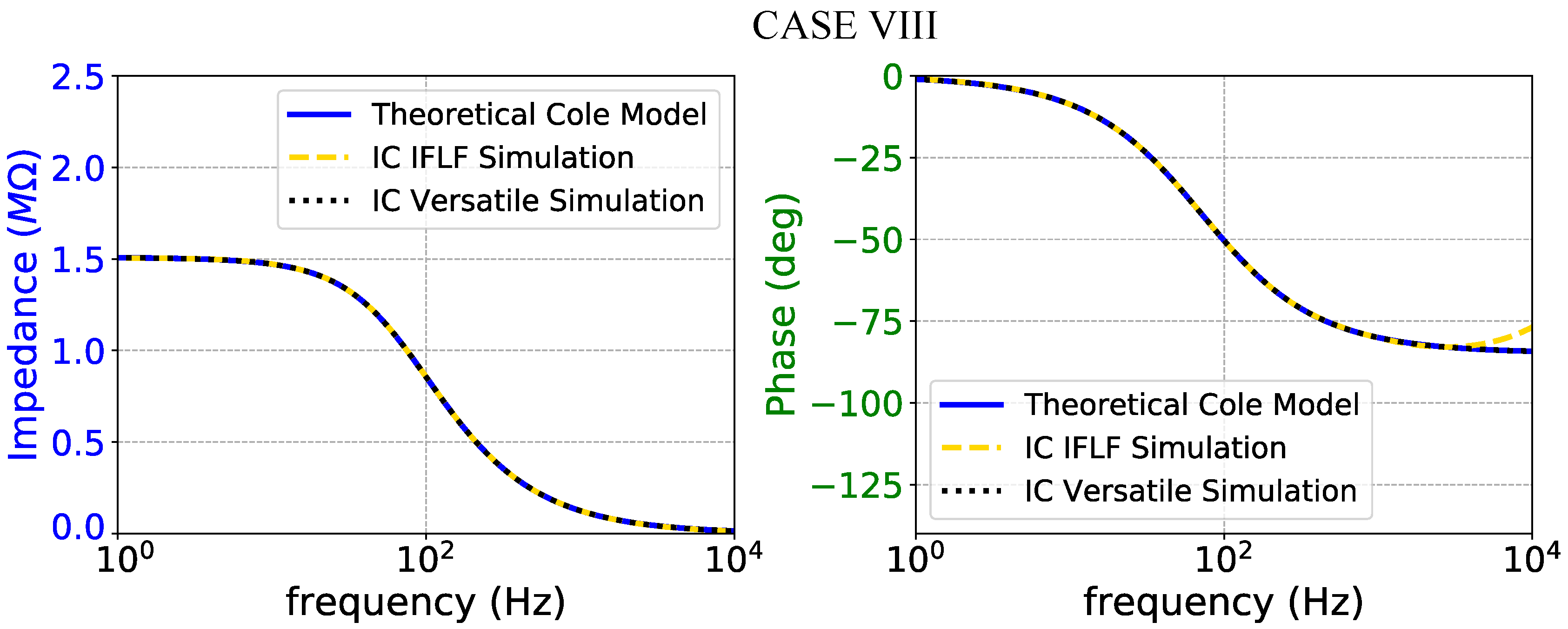
Figure 22.
Impedance magnitude (left) and phase response (right) of the case VIII fractional-order electrode model.
Figure 22.
Impedance magnitude (left) and phase response (right) of the case VIII fractional-order electrode model.
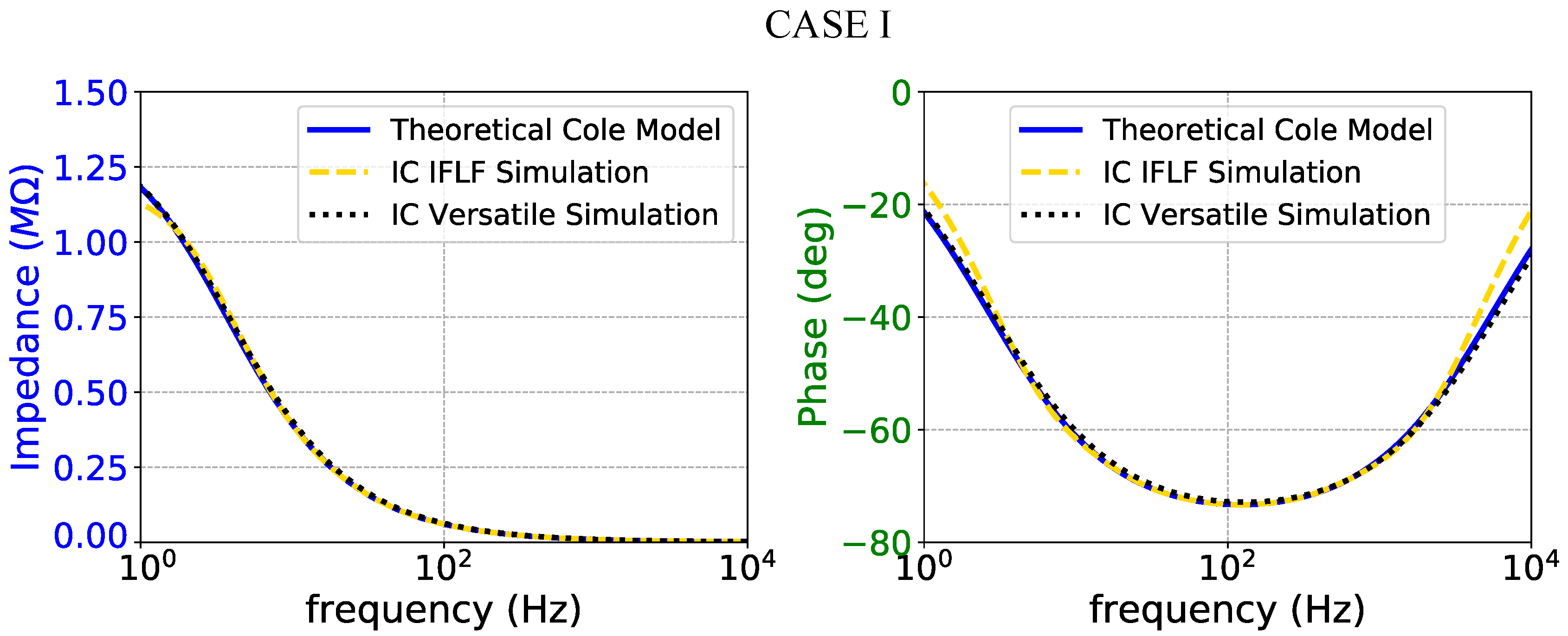
Figure 23.
Impedance magnitude (left) and phase response (right) of the case I fractional-order skin model.
Figure 23.
Impedance magnitude (left) and phase response (right) of the case I fractional-order skin model.
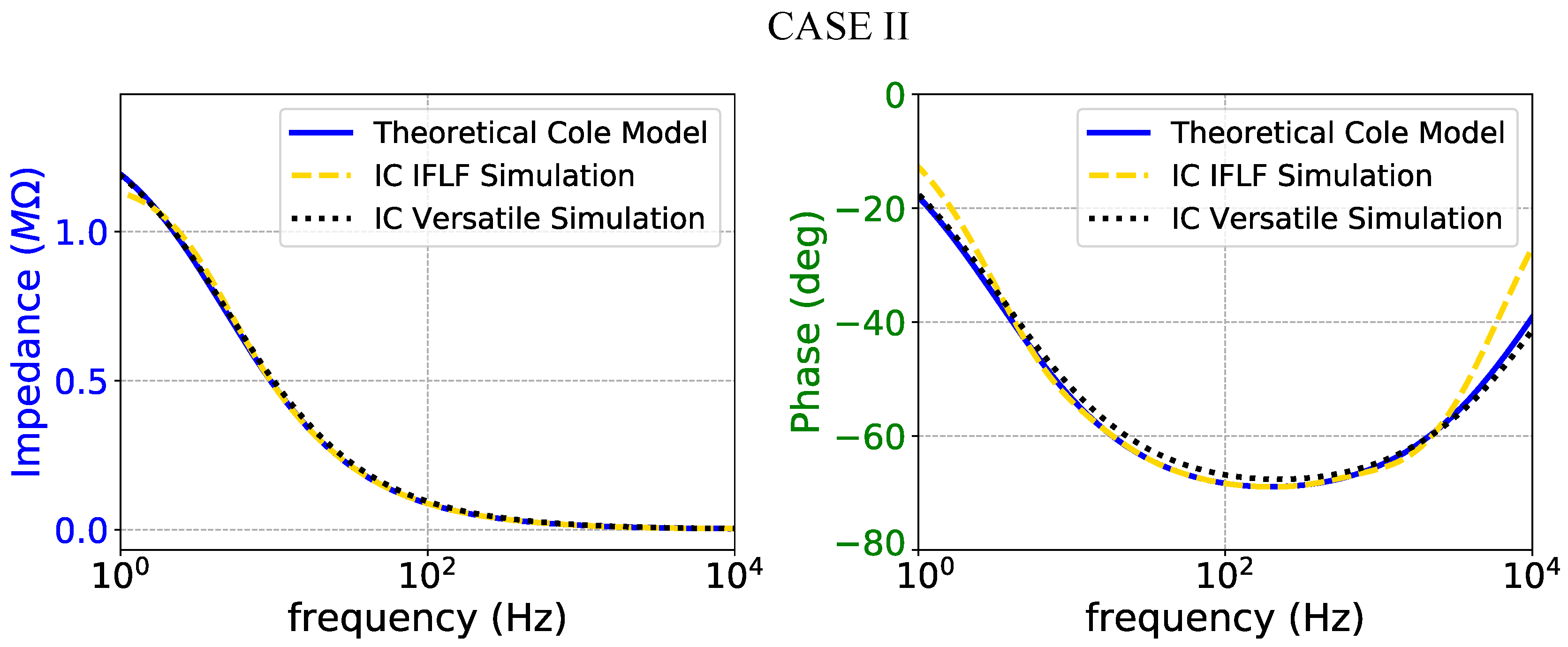
Figure 24.
Impedance magnitude (left) and phase response (right) of the case II fractional-order skin model.
Figure 24.
Impedance magnitude (left) and phase response (right) of the case II fractional-order skin model.
Figure 25.
Impedance magnitude (left) and phase response (right) of the case III fractional-order skin model.
Figure 25.
Impedance magnitude (left) and phase response (right) of the case III fractional-order skin model.
Figure 26.
Impedance magnitude (left) and phase response (right) of the case IV fractional-order skin model.
Figure 26.
Impedance magnitude (left) and phase response (right) of the case IV fractional-order skin model.
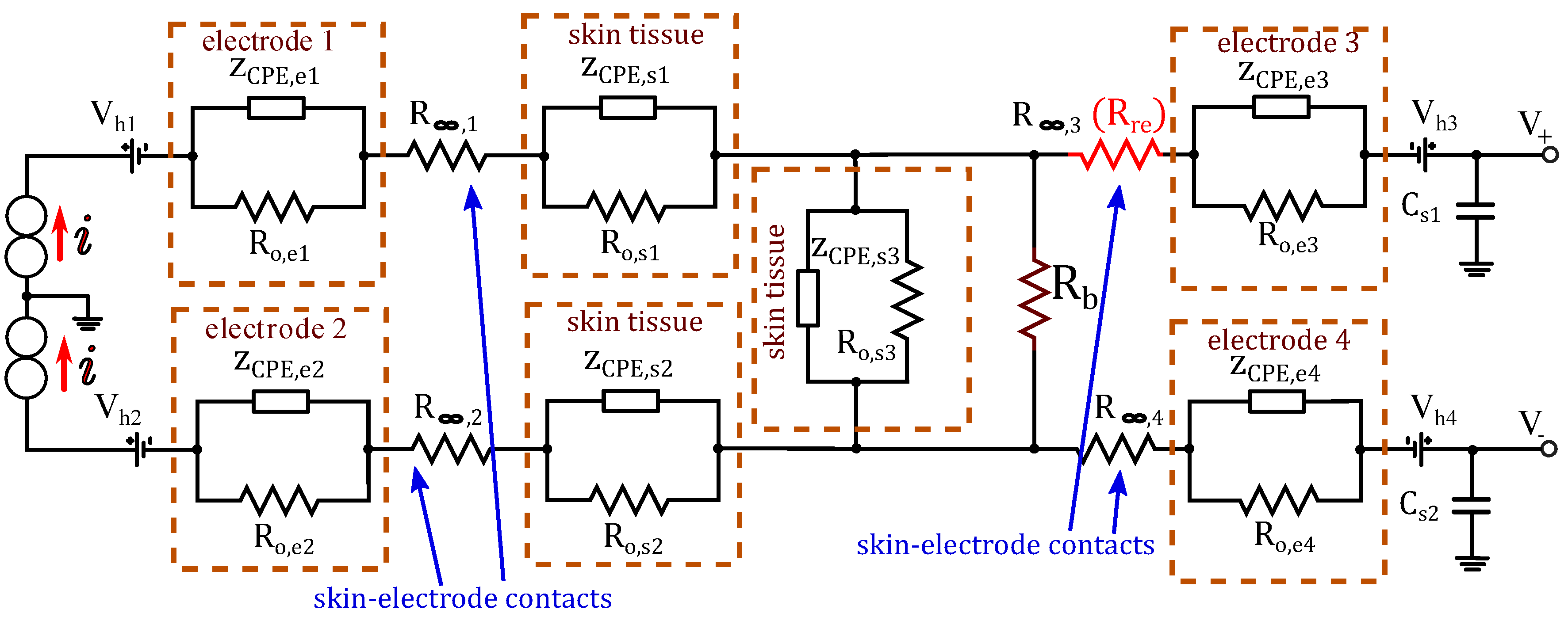
Figure 27.
Tetrapolar setup cases.
Figure 27.
Tetrapolar setup cases.
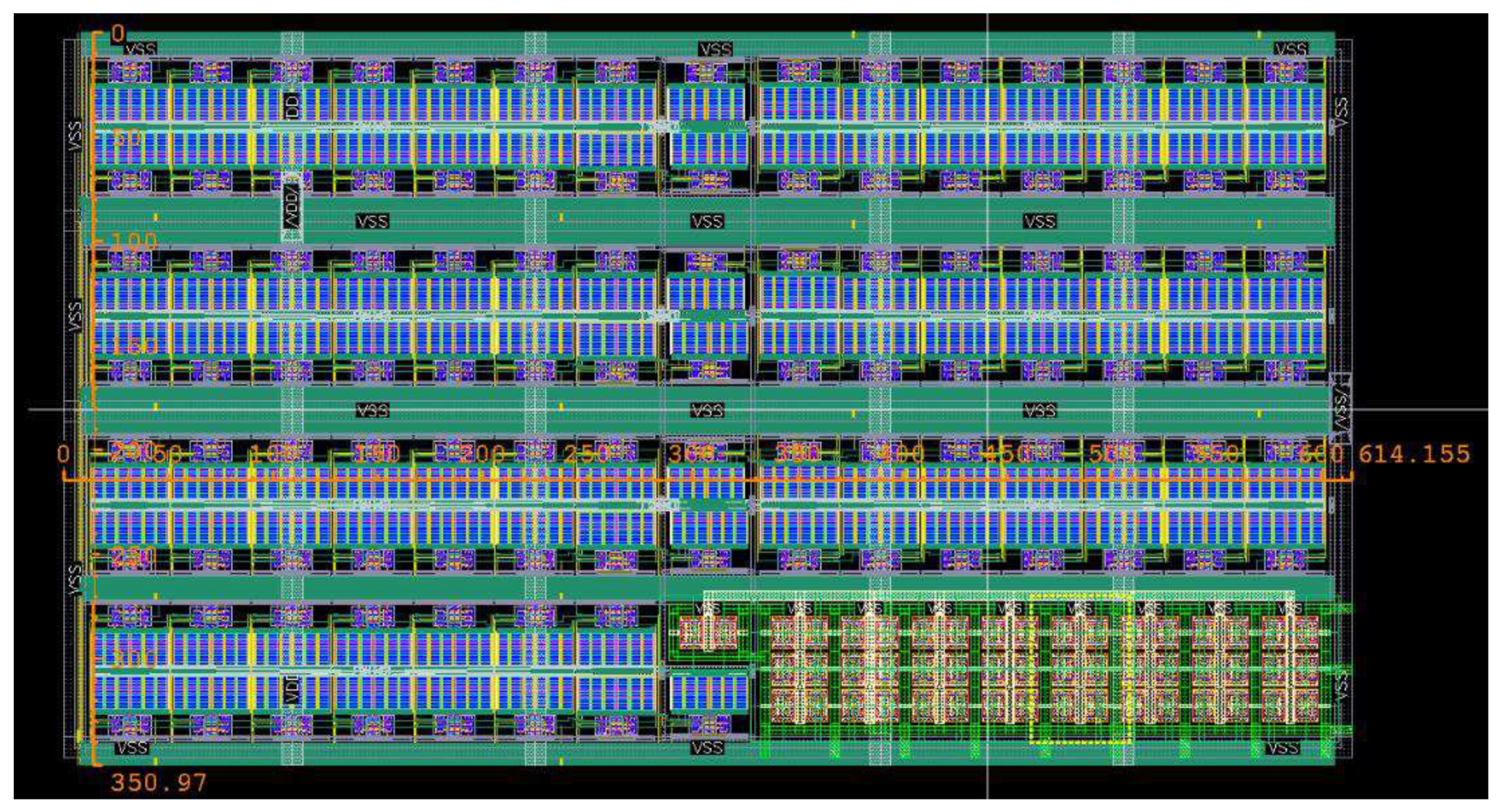
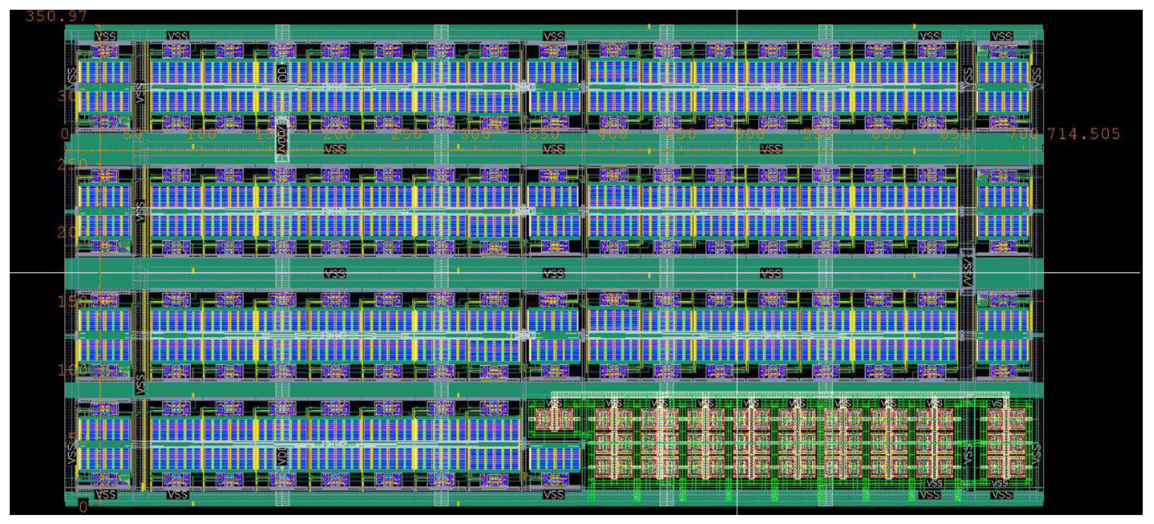
Figure 28.
Layout design of the implemented tetrapolar bioimpedance measurement.
Figure 28.
Layout design of the implemented tetrapolar bioimpedance measurement.
Figure 29.
Layout design of the implemented tetrapolar bioimpedance measurement.
Figure 29.
Layout design of the implemented tetrapolar bioimpedance measurement.
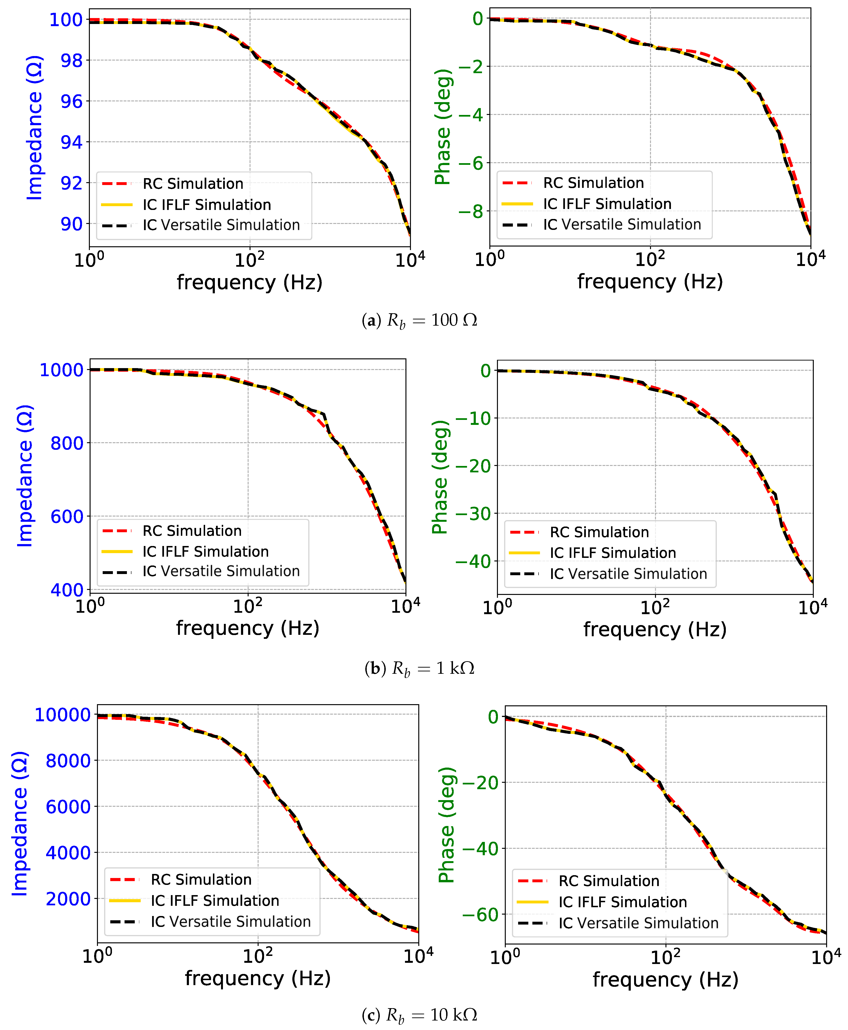
Figure 30.
AC magnitude and phase impedance measurements for (a) Rb = 100 Ω, (b) Rb = 1 kΩ, and
(c) Rb = 10 kΩ: all electrode and contact impedances are equal (R∞ = 1.5 kΩ). The corresponding RC
network approximations are included for comparison.
Figure 30.
AC magnitude and phase impedance measurements for (a) Rb = 100 Ω, (b) Rb = 1 kΩ, and
(c) Rb = 10 kΩ: all electrode and contact impedances are equal (R∞ = 1.5 kΩ). The corresponding RC
network approximations are included for comparison.
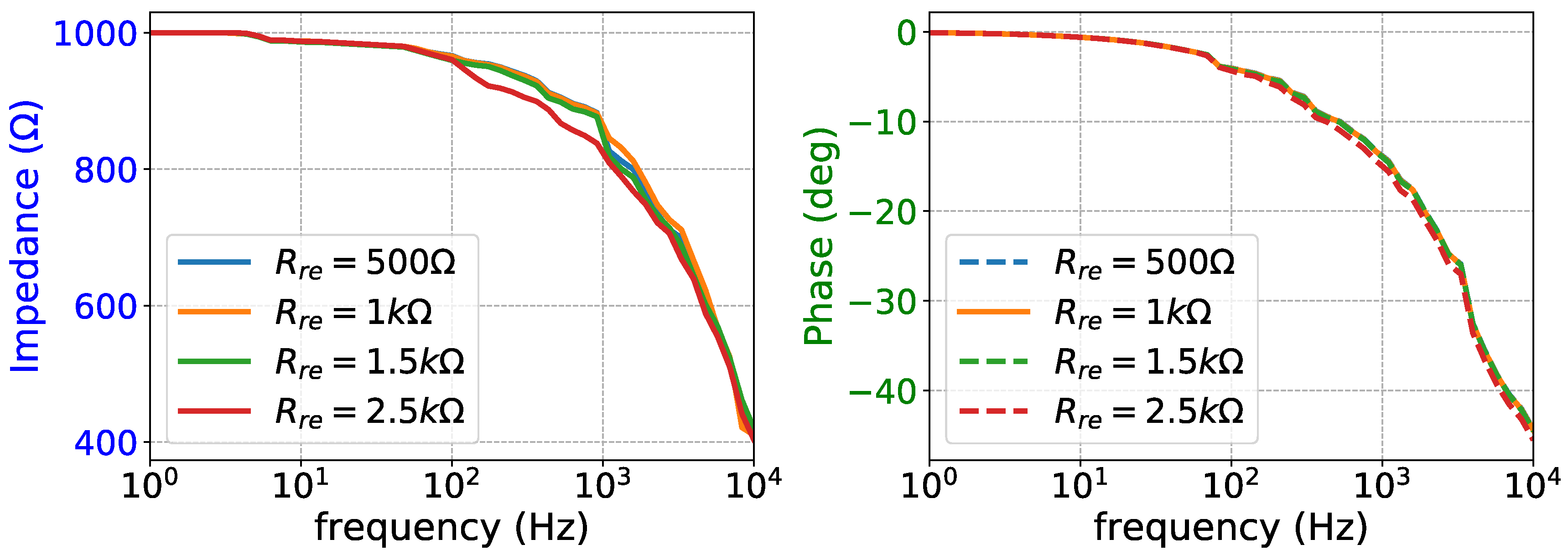
Figure 31.
AC magnitude (left) and phase (right) impedance measurements for deviated shunt impedance of the positive voltage electrode (versatile design).
Figure 31.
AC magnitude (left) and phase (right) impedance measurements for deviated shunt impedance of the positive voltage electrode (versatile design).
Figure 32.
AC magnitude (left) and phase (right) impedance measurements for deviated shunt impedance of the positive voltage electrode (IFLF design).
Figure 32.
AC magnitude (left) and phase (right) impedance measurements for deviated shunt impedance of the positive voltage electrode (IFLF design).
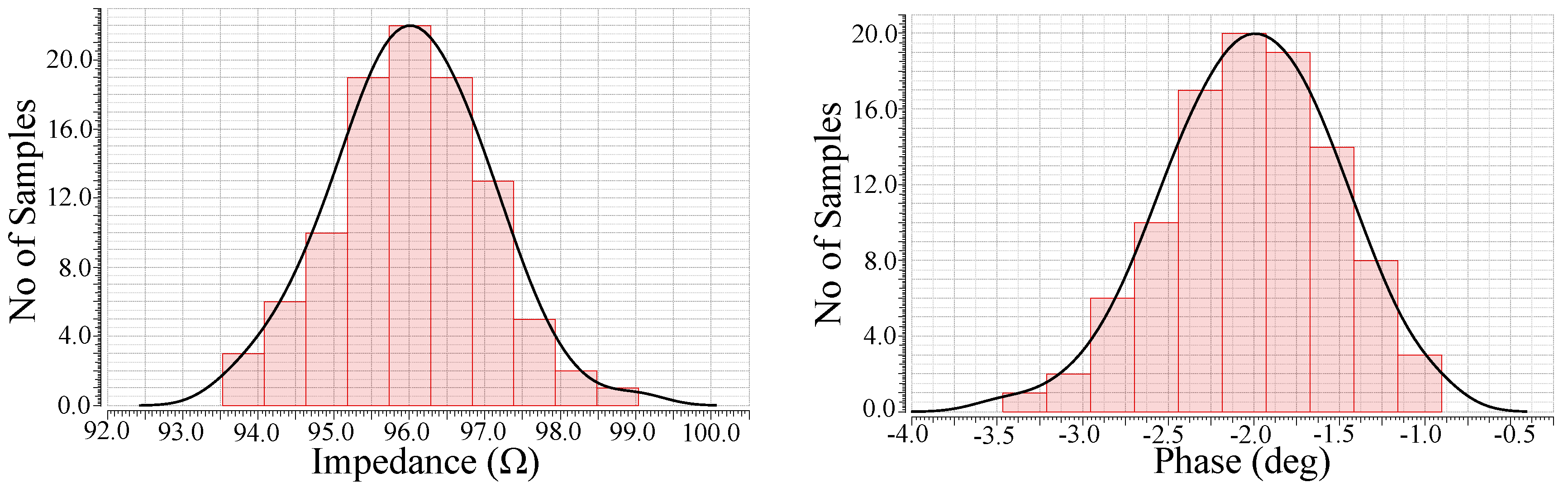
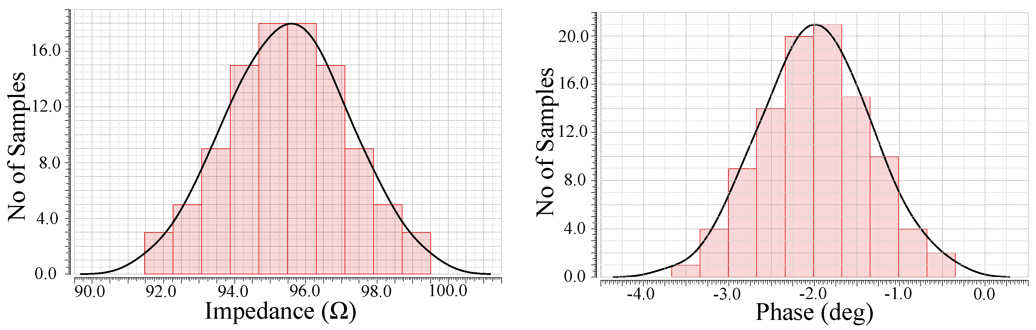
Figure 33.
Sensitivity performance of magnitude for target impedance using Monte-Carlo analysis (versatile design).
Figure 33.
Sensitivity performance of magnitude for target impedance using Monte-Carlo analysis (versatile design).
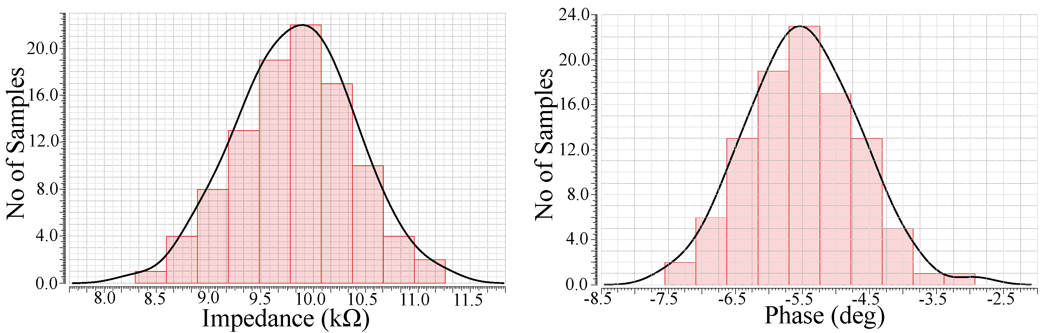
Figure 34.
Sensitivity performance of magnitude for target impedance using Monte-Carlo analysis (IFLF design).
Figure 34.
Sensitivity performance of magnitude for target impedance using Monte-Carlo analysis (IFLF design).
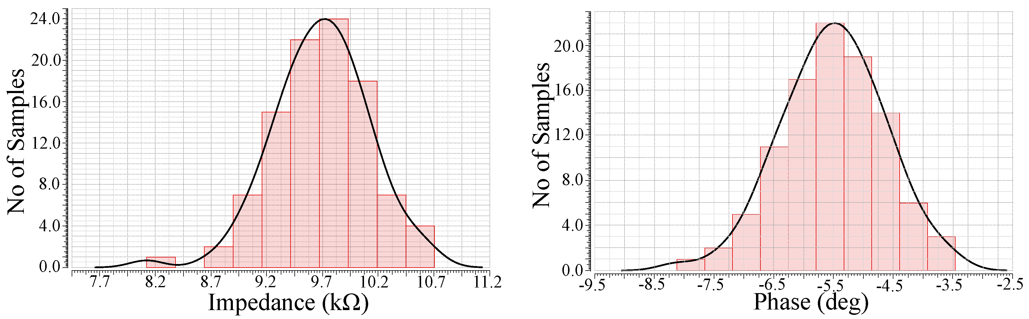
Figure 35.
Sensitivity performance of magnitude for target impedance k using Monte-Carlo analysis (versatile design).
Figure 35.
Sensitivity performance of magnitude for target impedance k using Monte-Carlo analysis (versatile design).
Figure 36.
Sensitivity performance of phase for target impedance k using Monte-Carlo analysis (versatile design).
Figure 36.
Sensitivity performance of phase for target impedance k using Monte-Carlo analysis (versatile design).
Table 1.
Skin (upper arm) and electrode Cole model typical parameter values [
16,
31].
Table 1.
Skin (upper arm) and electrode Cole model typical parameter values [
16,
31].
| Parameter | (k) | (M) | (s) | a | C (nF/sec) |
|---|
| Skin | 1.86 | 1.39 | 0.53 | 0.749 | 447 |
| Electrode | 0.21 | 1.08 | 1.41 | 0.942 | 1.92 |
Table 2.
Indicative skin and electrode Cole model parameter range [
16,
31,
32,
33,
34].
Table 2.
Indicative skin and electrode Cole model parameter range [
16,
31,
32,
33,
34].
| Parameter | (M) | a | C (nF/sec) |
|---|
| Skin | 0.64–1.46 | 0.63–0.86 | 61.2–1042.1 |
| Electrode | 0.65–2.09 | 0.8–0.99 | 1.39–2.09 |
Table 3.
Passive element values for approximating the fractional-order capacitors.
Table 3.
Passive element values for approximating the fractional-order capacitors.
| Electrode Element | Value | Skin Element | Value |
|---|
| pF | | nF |
| pF | | nF |
| pF | | nF |
| pF | | nF |
| pF | | nF |
| pF | | nF |
| M | | M |
| M | | k |
| M | | |
| k | | k |
| 100 k | | |
| G | | M |
Table 4.
Parameters for the implementation of expression H(s) (
12).
Table 4.
Parameters for the implementation of expression H(s) (
12).
| Electrode Parameter | Value | Skin Parameter | Value |
|---|
| | | |
| | | |
| | | |
| | | |
| | | |
| | | |
| | | |
| | | |
| | | |
| | | |
| | | |
| | | |
| | | |
Table 5.
MOS transistors dimensions—OTA and CCII.
Table 5.
MOS transistors dimensions—OTA and CCII.
| OTA | W/L (μm/μm) | CCII | W/L (μm/μm) |
|---|
| , | | , , | |
| – | | , | |
| – | | | |
| – | | - | |
| – | | | |
| , | | – | – |
Table 6.
Values of the capacitors of
Figure 4.
Table 6.
Values of the capacitors of
Figure 4.
| Element | Value | Element | Value |
|---|
| pF | | pF |
| pF | | nF |
| nF | | nF |
Table 7.
Values of the scaling factors .
Table 7.
Values of the scaling factors .
| Electrode Model Scaling Factor | Value | Skin Model Scaling Factor | Value |
|---|
| | | |
| | | |
| | | |
| | | |
| | | |
| | | |
Table 8.
Values of the capacitors of
Figure 7.
Table 8.
Values of the capacitors of
Figure 7.
| Element | Value | Element | Value |
|---|
| pF | | pF |
| pF | | nF |
| nF | - | - |
Table 9.
Values of transcoductance for the skin model of
Figure 7.
Table 9.
Values of transcoductance for the skin model of
Figure 7.
| Parameter | Value | Parameter | Value |
|---|
| nS | | nS |
| nS | | nS |
| nS | | nS |
| 55.37 μS | - | - |
Table 10.
Values of the scaling factors .
Table 10.
Values of the scaling factors .
| Electrode Model Scaling Factor | Value | Skin Model Scaling Factor | Value |
|---|
| | | |
| | | |
| | | |
| | | |
| | | |
| | | |
Table 11.
Electrode Cole parameters values for different cases, .
Table 11.
Electrode Cole parameters values for different cases, .
| Case/Parameter | (M) | (nF/sec) |
|---|
| Case I | 1.08 | 1.75 |
| Case II | 2.09 | 1.39 |
| Case III | 0.65 | 1.92 |
| Case IV | 1.51 | 1.92 |
| Case V | 0.65 | 1.75 |
| Case VI | 1.51 | 1.75 |
| Case VII | 0.65 | 2.09 |
| Case VIII | 1.51 | 2.09 |
Table 12.
Skin Cole parameters values for different cases, M.
Table 12.
Skin Cole parameters values for different cases, M.
| Case/Parameter | | (nF/sec) |
|---|
| Case I | 0.86 | 65.2 |
| Case II | 0.81 | 61.2 |
| Case III | 0.82 | 88.9 |
| Case IV | 0.78 | 73.1 |


