Abstract
Voltage-mode and current-mode fractional-order filter topologies, which are capable of realizing various types of transfer functions, are introduced in this paper. Thanks to the employment of the transconductance parameter of the MOS transistors, the derived filter structures offer the benefit of the electronic adjustment of their frequency characteristics. With regards to the literature, the number of MOS transisitors is minimized leading to significant reduction of the circuit complexity and power dissipation. Simulation results, derived using the Design Kit of the 0.35 μm Austria Mikro Systeme CMOS process and the Cadence IC design suite, confirm the correct operation of the presented filter structures.
1. Introduction
Owing to the interdisciplinary nature of fractional-order calculus [1,2,3], the development of fractional-order filters has gained a significant research interest because of the offered more precise gradient of the transition from pass-band to stop-band, with regards to their integer-order counterparts. This originates from the fact that the slope of the attenuation of an order filter, with n integer and , is equal to dB/Oct., instead of dB/Oct. slope realized by the corresponding integer-order filters [4]. Another benefit of the fractional-order filters is their capability of performing scaling of the realized time-constants due to their dependence on the order of the filter. This is a very attractive feature in the case of biomedical applications, where very large values of time-constants are required [5].
Due to the absence of commercially available fractional-order capacitors [6,7,8], fractional-order filters can be derived through: (a) the substitution of the conventional (i.e., integer-order) capacitors in the well-known integer-order filters with RC networks (e.g., Foster or Cauer) [9,10], and (b) the implementation of the rational integer-order transfer functions, which are derived through the substitution of the Laplacian fractional-order operator with a suitable expression offered by approximation formulas such as Oustaloup, Continued Fraction Expansion, Matsuda, El-Khazali etc. [11,12,13,14,15,16]. Comparing the aforementioned methods, the main derivation is that the first one offers a quick design procedure but the resulting filter structures suffer from the absence of electronic tuning of the employed RC networks; the second one offers fully electronic tunability of the characteristics of the fractional-order filters. On the other hand, the active component count is much higher in this case and, consequently, the circuit complexity and the power dissipation are both increased [5].
Fractional-order filters, implemented using various types of active elements such as Operational Amplifiers (op-amps), Operational Transconductance Amplifiers (OTAs), second generation Current Conveyors (CCIIs), Current-Feedback Operational Amplifiers (CFOAs) and current-mirrors (CMs), have been already proposed in the literature [17,18,19,20,21,22,23,24,25,26,27,28,29,30,31,32,33,34,35,36]. All of them suffer from the increased number of MOS transistors which are required for implementing the active elements. In addition, only the filter realizations performed with OTAs or CMs offer the benefit of the electronic adjustment of the frequency characteristics, due to the employment of the transconductance parameter () of the MOS transistors.
The contribution made in this work is the introduction of fractional-order voltage-mode and current-mode filter topologies, constructed from a minimum number of MOS transistors with regards to those required in the already published topologies. The proposed structures are capable of providing low-pass, high-pass, and band-pass filter functions and, consequently, they are multi-function schemes being attractive due to their design versatility and flexibility. Due to the realization of time-constants through the employment of the electronically controlled transconductance parameter, their characteristic frequencies can be electronically adjusted by the corresponding dc bias currents.
The paper is organized as follows: a short introduction on the fractional-order filter characteristics is given in Section 2, while the proposed implementations are presented in Section 3. Their performance evaluation is provided in Section 4, through simulation results obtained using the Cadence IC design suite and the MOS transistor parameters provided by the Austrian Mikro Systeme (AMS) CMOS 0.35 μm Design Kit.
2. Fractional-Order Filters
The transfer function of a fractional low-pass filter of order is
with variable being the time-constant, associated to the pole frequency () through the relationship: [31].
Setting in (1), the expressions of the gain and phase responses are given by (2) and (3), respectively
The maximum gain of the filter is equal to 1 for , while the slope of the stop-band attenuation is equal to dB/Oct. Defining as half-power frequency () the frequency where a 3 dB drop from the maximum gain is observed, the expressions of this frequency as well as of the phase at this frequency, derived from (2) and (3), are provided by the Equations (4) and (5), respectively
According to (4), the pole frequency is different from the half-power frequency and not equal, as in the case of conventional integer-order filters. As the half-power frequency depends on the order of the filter, scaling of the time-constant is possible by adjusting the order of the filter. For example, this is very useful in biomedical applications where extremely small cut-off frequencies are required.
A fractional high-pass filter of order is described by the the transfer function in (6)
The expressions of the magnitude and phase responses are
The maximum gain of the filter is equal to 1 for while the slope of the gradient from stop-band to pass-band is equal to dB/Oct.
The half-power frequency is given by the expression in (9)
and the observations made in the case of the low-pass filter, about the dependence of the half-power frequency on the order, are still valid. The phase at this frequency is given by (10)
A fractional-order band-pass filter is described by the transfer function
where the order of the band-pass filter is equal to . The slope of the gradient at low frequencies is dB/Oct., while at high-frequencies the slope becomes dB/Oct., giving the capability of implementing asymmetric band-pass filters with controlled slopes in both low and high frequency ranges.
The peak frequency of the band-pass filter () is calculated through the condition: , while the lower () and upper () cut-off frequencies are calculated by setting: . Moreover, the realized quality factor (Q) is given by the formula: [36].
3. Proposed Implementations
3.1. Voltage-Mode Filters
As it was mentioned in Section 1, OTA-C implementations are attractive due to the offered electronic tuning which originates from the control of the transconductance parameter by the associated bias current [37]. Considering that the impedance of a fractional-order capacitor is given by (12)
with being the pseudo-capacitance expressed in Farad/sec, and that the transconductance of OTAs is , then the OTA-C filters depicted in Figure 1a,b implement the transfer functions in (1) and (6), respectively. The realized time-constant is given by the formula:
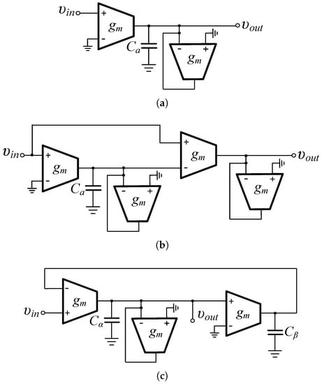
Figure 1.
Realization of voltage-mode fractional-order (a) low-pass, (b) high-pass, and (c) band-pass filters using OTAs as active elements.
The two-integrator loop OTA-C filter in Figure 1c implements the following band-pass filter function
with the time-constant given by the formula:
In order to reduce the MOS transistor count, the proposed topology is demonstrated in Figure 2a [38]. Considering that transistors Mp1-Mp2 are matched, with transconductance parameter equal to , the derived transfer functions are:
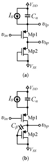
Figure 2.
Proposed voltage-mode fractional-order (a) low-pass and high-pass, and (b) band-pass filter topologies.
Comparing (1) with (14) and (6) with (15), it is readily observed that the topology in Figure 2a implements low-pass and high-pass filter functions, with the time-constant given by (16)
3.2. Current-Mode Filters
The implementation of current-mode low-pass and high-pass filters, using OTAs as active elements, is demonstrated in Figure 3a,b, where the topologies implement the transfer functions in (14) and (15), respectively. The implementation of the band-pass filter is performed by the topology in Figure 3c, which realizes the transfer function in (13).
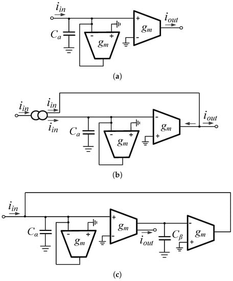
Figure 3.
Realization of current-mode fractional-order (a) low-pass, (b) high-pass, and (c) band-pass filters using OTAs as active elements.
The proposed current-mode low-pass filter structure is depicted in Figure 4a. Applying the Kirchhoff’s current law (KCL) at the input terminal and taking into account the current-mirror operation, implemented by transistors Mn1–Mn2, it is derived that
with being the current that flows through the capacitor , given by the formula
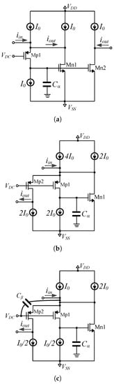
Figure 4.
Proposed current-mode fractional-order (a) low-pass, (b) high-pass, and (c) band-pass filters.
Considering that is the transconductance of Mn1–Mn2, the output current is expressed as
Using (19)–(21) it is derived that the topology in Figure 4a implements the transfer function in (14) with a time-constant given by (22)
Let us consider the topology in Figure 4b; applying the KCL at the input terminal and assuming that Mp1–Mp2 are matched transistors forming a current-mirror with ac current equal to , it is obtained that
In addition, the current that flows through the capacitor is
Inspecting (25) it is readily obtained that the topology in Figure 4b implements a high-pass filter function with the time-constant given by (22).
The topology in Figure 4c is derived by adding an extra fractional-order capacitor () in the topology of Figure 4b. The KCL at the input node takes the form
The current that flows through the capacitor is still given by (24), while for the capacitor the following expression is valid
4. Simulation and Comparison Results
The behavior of the proposed topologies will be evaluated using the Cadence IC design suite and the Design Kit provided by the AMS 0.35 m CMOS process. The power supply voltages were V. Considering the fourth-order Foster-II network given in Figure 5 and using the Continued Fraction Expansion approximation with center frequency 10 Hz and the Matlab code introduced in [39], then the values of the passive element values of the RC network for approximating fractional-order capacitances () of orders with values 85.4 nF/sec, 37.4 nF/sec, and 16.3 nF/sec, are provided in Table 1.
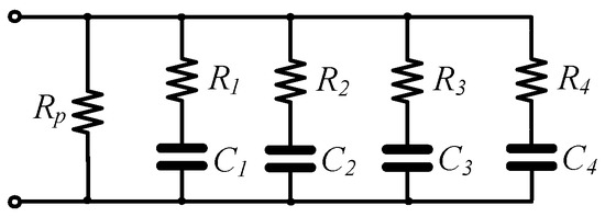
Figure 5.
RC network for approximating the fractional-order capacitors in the proposed fractional-order filter topologies.

Table 1.
Values of passive elements of the network in Figure 5.
Considering MOS transistors biased in the sub-threshold region, their transconductance is given by (29)
where 1 < n < 2 is the sub-threshold slope factor of a MOS transistor, is the thermal voltage (26 mV @ 27 C), and is the bias current [40,41]. Thus, the realized-time constants are electronically adjusted, offering the capability of electronic adjustment of the frequency characteristics of the realized filter functions.
4.1. Voltage-Mode Filters
Assuming a dc bias current equal to = 10 nA, the aspect ratio of Mp1–Mp2 in Figure 2 was chosen to be 100 m/1 m, in order to guarantee operation in the sub-threshold region.
The obtained frequency magnitude and phase responses of the low-pass and high-pass filters are provided in Figure 6, while the corresponding theoretically predicted plots are given by dashes. The most important performance characteristics are given in Table 2 and Table 3, along with the theoretical values given between parentheses.
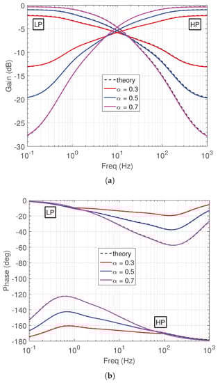
Figure 6.
Simulated frequency responses of the proposed voltage-mode low-pass and high-pass filters in Figure 2a (a) gain, and (b) phase.
Table 2.
Frequency characteristics of the low-pass filter in Figure 2a.
Table 3.
Frequency characteristics of the high-pass filter in Figure 2a.
The electronic tuning capability of the filter structure in Figure 2a has been evaluated by considering the set of bias currents nA. The obtained frequency responses are depicted in Figure 7, where the values of the half-power frequency were Hz for the low-pass filter and Hz for the high-pass filter.
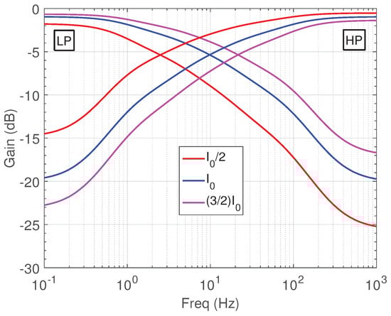
Figure 7.
Demonstration of the electronic tuning capability of the filter structure in Figure 2a.
According to (4), (9), (16) and (29), the half-power frequencies and , which correspond to bias currents and , are related according to the expression given by (30)
Therefore, the theoretically predicted values will be Hz and Hz, respectively, confirming the aforementioned feature.
The effects of MOS transistor parameters mismatch, as well as those of the process parameter variations, have been evaluated using the Monte Carlo analysis tool (N = 100 runs) offered by the Analog Design Environment of the Cadence software. The derived statistical plots for order are provided in Figure 8, while the values of standard deviation of the half-power frequency were Hz for the low-pass filter and Hz for the high-pass filter, confirming that the proposed structure has reasonable sensitivity characteristics.
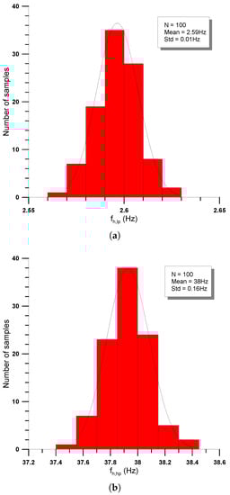
Figure 8.
Statistical plots about the sensitivity of the half-power frequency in the case of the voltage-mode (a) low-pass, and (b) high-pass filters of order .
In order to estimate which circuit element contributes to the maximum error, a sensitivity analysis has been performed through the Cadence software. According to this analysis, it is derived that the deviations in the measurement of the half-power frequency as well as of the maximum gain in both low-pass and high-pass filter topologies of Figure 2a, are caused by transistor Mp1.
The evaluation of the performance of the band-pass filter in Figure 2b has been performed by considering that the orders () are . The derived frequency responses are depicted in Figure 9, while the results in Table 4 confirm the correct operation of the filter.
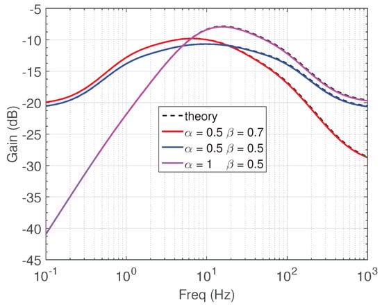
Figure 9.
Frequency responses of the band-pass filter in Figure 2b for various orders.
Table 4.
Frequency characteristics of the band-pass filter in Figure 2b.
4.2. Current-Mode Filters
The power supply voltages and capacitor values which will be considered in the performance evaluation of the current-mode filters will be the same as in the case of the voltage-mode filters. In addition, the value of the dc voltage will be equal to 150 mV.
The frequency responses of the current-mode low-pass (Figure 4a) and high-pass (Figure 4b) filters are provided in Figure 10. The results in Table 5 and Table 6, where the theoretically predicted values are given between parentheses, confirm the accurate operation of the proposed filters.
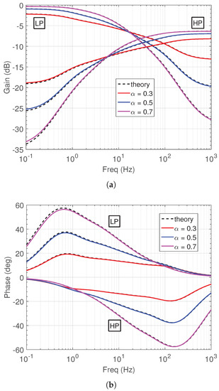
Table 5.
Frequency characteristics of the low-pass filter in Figure 4a.
Table 6.
Frequency characteristics of the high-pass filter in Figure 4b.
The electronic tuning capability of the filters for is demonstrated in Figure 11, where for bias currents nA, for the low-pass filter the corresponding half-power frequencies were Hz, while for the high-pass filter the derived half-power frequencies were Hz. These results are close to the results Hz and Hz, which are derived according to (30).
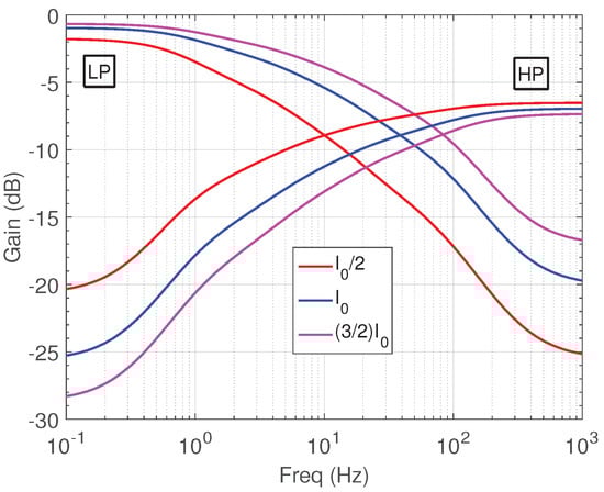
Figure 11.
Demonstration of the electronic tuning capability of the current-mode low-pass and high-pass filters.
The sensitivity behavior of the filters has been evaluated using the Monte Carlo analysis tool (N = 100 runs) and the derived values of standard deviation of the half-power frequency were Hz for the low-pass filter and Hz for the high-pass filter. The obtained statistical plots for order are provided in Figure 12.
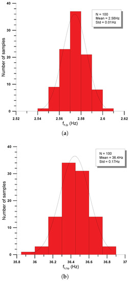
Figure 12.
Statistical plots about the sensitivity of the half-power frequency in the case of the current-mode (a) low-pass, and (b) high-pass filters of order .
Performing also a sensitivity analysis, the obtained results showed that for the low-pass filter topology in Figure 4a, the obtained error in the measurement of the half-power frequency is caused by Mn1, while transistors Mn1 and Mn2 equally contribute in the error of the low frequency gain. In the case of the high-pass filter circuit of Figure 4b, transistors Mp1 and Mp2 equally contribute to the derived deviations in the measurement of the half-power frequency as well as of the high frequency gain.
The frequency responses of band-pass filter functions that correspond to orders () equal to are presented in Figure 13, while the corresponding simulated values of the most important characteristics are given in Table 7.
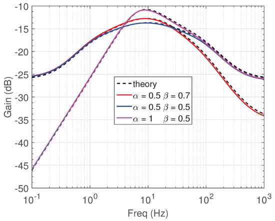
Figure 13.
Frequency responses of the current mode band-pass filter for various orders.
Table 7.
Frequency characteristics of the current-mode band-pass filter.
4.3. Comparison Results
In order to perform a comparison between the MOS transistor count needed for implementing the OTA-C filters and the proposed structures, let us consider the typical OTA topology provided in Figure 14. Here 9 MOS transistors are required for its implementation and the dc power dissipation, considering that , is equal to .
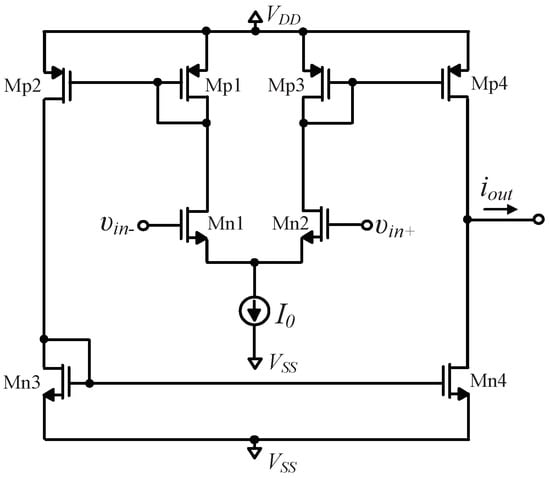
Figure 14.
Typical OTA structure.
The derived comparison results between the proposed voltage-mode and current-mode filters are summarized in Table 8 and Table 9, respectively. According to the provided results, it is concluded that both types of implementations offer reduced MOS transistor count, which means reduced circuit complexity, and lower dc power dissipation.
Table 8.
Comparison between the MOS transistor count and dc power dissipation for the proposed voltage-mode filters.
Table 9.
Comparison between the MOS transistor count and dc power dissipation for the proposed current-mode filters.
5. Conclusions
The proposed voltage-mode and current-mode filter structures offer significant reduction of circuit complexity and dc power dissipation, with regards to their OTA-C counterparts. In the case of voltage-mode filters, the reduction in the number of transistors is 83.3%, 91.6%, and 88.9% for low-pass, high-pass and band-pass filters, respectively. The achieved reduction of the dc power dissipation is 75%, 87.5%, and 83.3%, respectively. In the case of current-mode filters, the corresponding factors are 61.1% MOS transistor count reduction for both low-pass and high-pass filters, while for the band-pass filters, the corresponding value is 74.1%. With regards to the power dissipation, the corresponding factors are 25% for both low-pass and high-pass filters, and 50% for the band-pass filter. Therefore, the proposed structures are attractive candidates for implementing fractional-order filters with low complexity and reduced power dissipation.
Author Contributions
Conceptualization, C.P., A.S.E. and B.M.; methodology, C.P. and A.S.E.; validation, P.B.; formal analysis, P.B.; investigation, C.P. and P.B.; writing—original draft preparation, C.P. and P.B.; writing—review and editing, A.S.E. and B.M.; supervision: C.P.
Funding
This research received no external funding.
Acknowledgments
This work is supported by the General Secretariat for Research and Technology (GSRT) and the Hellenic Foundation for Research and Innovation (HFRI). This article is based upon work from COST Action CA15225, a network supported by COST (European Cooperation in Science and Technology).
Conflicts of Interest
The authors declare no conflict of interest.
Abbreviations
The following abbreviations are used in this manuscript:
| MOS | Metal-Oxide-Semiconductor |
| CMOS | Complementary Metal-Oxide-Semiconductor |
| IC | Integrated Circuit |
| RC | Resistor Capacitor |
| OP-AMP | Operational Amplifier |
| OTA | Operational Transconductance Amplifier |
| CCII | Second-generation Current Conveyor |
| CFOA | Current Feedback Operational Amplifier |
| CM | Current-Mirrors |
References
- Hidalgo-Reyes, J.; Gómez-Aguilar, J.F.; Escobar-Jiménez, R.F.; Alvarado-Martínez, V.M.; López-López, M.G. Classical and fractional-order modeling of equivalent electrical circuits for supercapacitors and batteries, energy management strategies for hybrid systems and methods for the state of charge estimation: A state of the art review. Microelectron. J. 2019, 85, 109–128. [Google Scholar] [CrossRef]
- Morales-Delgado, V.F.; Gómez-Aguilar, J.F.; Taneco-Hernández, M.A.; Escobar-Jiménez, R.F. Fractional operator without singular kernel: Applications to linear electrical circuits. Int. J. Circuit Theory Appl. 2018, 46, 2394–2419. [Google Scholar] [CrossRef]
- Sun, H.G.; Zhang, Y.; Baleanu, D.; Chen, W.; Chen, Y.Q. A new collection of real world applications of fractional calculus in science and engineering. Commun. Nonlinear Sci. Numer. Simul. 2018, 64, 213–231. [Google Scholar] [CrossRef]
- Elwakil, A.S. Fractional-order circuits and systems: An emerging interdisciplinary research area. IEEE Circuits Syst. Mag. 2010, 10, 40–50. [Google Scholar] [CrossRef]
- Tsirimokou, G.; Psychalinos, C.; Elwakil, A. Design of CMOS Analog Integrated Fractional-Order Circuits: Applications in Medicine and Biology; Springer: Berlin/Heidelberger, Germany, 2017. [Google Scholar] [CrossRef]
- Agambayev, A.; Farhat, M.; Patole, S.P.; Hassan, A.H.; Bagci, H.; Salama, K.N. An ultra-broadband single-component fractional-order capacitor using MoS2-ferroelectric polymer composite. Appl. Phys. Lett. 2018, 113, 093505. [Google Scholar] [CrossRef]
- Biswas, K.; Caponetto, R.; Di Pasquale, G.; Graziani, S.; Pollicino, A.; Murgano, E. Realization and characterization of carbon black based fractional order element. Microelectron. J. 2018, 82, 22–28. [Google Scholar] [CrossRef]
- Caponetto, R.; Di Pasquale, G.; Graziani, S.; Murgano, E.; Pollicino, A. Realization of Green Fractional Order Devices by using Bacterial Cellulose. AEU Int. J. Electron. Commun. 2019, 112, 152927. [Google Scholar] [CrossRef]
- Carlson, G.; Halijak, C. Approximation of fractional capacitors (1/s)ˆ(1/n) by a regular Newton process. IEEE Trans. Circuit Theory 1964, 11, 210–213. [Google Scholar] [CrossRef]
- Valsa, J.; Vlach, J. RC models of a constant phase element. Int. J. Circuit Theory Appl. 2013, 41, 59–67. [Google Scholar] [CrossRef]
- Oustaloup, A.; Levron, F.; Mathieu, B.; Nanot, F.M. Frequency-band complex noninteger differentiator: Characterization and synthesis. IEEE Trans. Circuits Syst. I Fundam. Theory Appl. 2000, 47, 25–39. [Google Scholar] [CrossRef]
- Krishna, B. Studies on fractional order differentiators and integrators: A survey. Signal Process. 2011, 91, 386–426. [Google Scholar] [CrossRef]
- Matsuda, K.; Fujii, H. H∞ optimized wave-absorbing control-Analytical and experimental results. J. Guid. Control Dyn. 1993, 16, 1146–1153. [Google Scholar] [CrossRef]
- El-Khazali, R. On the biquadratic approximation of fractional-order Laplacian operators. Analog. Integr. Circuits Signal Process. 2015, 82, 503–517. [Google Scholar] [CrossRef]
- AbdelAty, A.; Elwakil, A.; Radwan, A.; Psychalinos, C.; Maundy, B. Approximation of the fractional-order Laplacian sα as a weighted sum of first-order high-pass filters. IEEE Trans. Circuits Syst. II Express Briefs 2018, 65, 1114–1118. [Google Scholar] [CrossRef]
- Tsirimokou, G.; Kartci, A.; Koton, J.; Herencsar, N.; Psychalinos, C. Comparative study of discrete component realizations of fractional-order capacitor and inductor active emulators. J. Circuits Syst. Comput. 2018, 27, 1850170. [Google Scholar] [CrossRef]
- Adhikary, A.; Sen, S.; Biswas, K. Practical realization of tunable fractional order parallel resonator and fractional order filters. IEEE Trans. Circuits Syst. I Regul. Pap. 2016, 63, 1142–1151. [Google Scholar] [CrossRef]
- Baxevanaki, K.; Kapoulea, S.; Psychalinos, C.; Elwakil, A.S. Electronically tunable fractional-order highpass filter for phantom electroencephalographic system model implementation. AEU Int. J. Electron. Commun. 2019, 110, 152850. [Google Scholar] [CrossRef]
- Bertsias, P.; Psychalinos, C.; Elwakil, A.; Safari, L.; Minaei, S. Design and application examples of CMOS fractional-order differentiators and integrators. Microelectron. J. 2019, 83, 155–167. [Google Scholar] [CrossRef]
- Bertsias, P.; Psychalinos, C.; Maundy, B.J.; Elwakil, A.S.; Radwan, A.G. Partial fraction expansion-based realizations of fractional-order differentiators and integrators using active filters. Int. J. Circuit Theory Appl. 2019, 47, 513–531. [Google Scholar] [CrossRef]
- Dimeas, I.; Tsirimokou, G.; Psychalinos, C.; Elwakil, A.S. Experimental verification of fractional-order filters using a reconfigurable fractional-order impedance emulator. J. Circuits Syst. Comput. 2017, 26, 1750142. [Google Scholar] [CrossRef]
- Dvorak, J.; Langhammer, L.; Jerabek, J.; Koton, J.; Sotner, R.; Polak, J. Synthesis and Analysis of Electronically Adjustable Fractional-Order Low-Pass Filter. J. Circuits Syst. Comput. 2018, 27, 1850032. [Google Scholar] [CrossRef]
- Freeborn, T.J.; Maundy, B.; Elwakil, A.S. Field programmable analogue array implementation of fractional step filters. IET Circuits Devices Syst. 2010, 4, 514–524. [Google Scholar] [CrossRef]
- Jerabek, J.; Sotner, R.; Dvorak, J.; Polak, J.; Kubanek, D.; Herencsar, N.; Koton, J. Reconfigurable fractional-order filter with electronically controllable slope of attenuation, pole frequency and type of approximation. J. Circuits Syst. Comput. 2017, 26, 1750157. [Google Scholar] [CrossRef]
- Kapoulea, S.; Psychalinos, C.; Elwakil, A.S. Single active element implementation of fractional-order differentiators and integrators. AEU Int. J. Electron. Commun. 2018, 97, 6–15. [Google Scholar] [CrossRef]
- Kaskouta, E.; Kamilaris, T.; Sotner, R.; Jerabek, J.; Psychalinos, C. Single-Input Multiple-Output and Multiple-Input Single-Output Fractional-Order Filter Designs. In Proceedings of the 2018 41st International Conference on Telecommunications and Signal Processing (TSP), Athens, Greece, 4–6 July 2018; pp. 1–4. [Google Scholar]
- Khateb, F.; Kubánek, D.; Tsirimokou, G.; Psychalinos, C. Fractional-order filters based on low-voltage DDCCs. Microelectron. J. 2016, 50, 50–59. [Google Scholar] [CrossRef]
- Koton, J.; Kubanek, D.; Sladok, O.; Vrba, K.; Shadrin, A.; Ushakov, P. Fractional-Order Low-and High-Pass Filters Using UVCs. J. Circuits Syst. Comput. 2017, 26, 1750192. [Google Scholar] [CrossRef]
- Koton, J.; Kubanek, D.; Herencsar, N.; Dvorak, J.; Psychalinos, C. Designing constant phase elements of complement order. Analog Integr. Circuits Signal Process. 2018, 97, 107–114. [Google Scholar] [CrossRef]
- Langhammer, L.; Sotner, R.; Dvorak, J.; Domansky, O.; Jerabek, J.; Uher, J. A 1+ α Low-Pass Fractional-Order Frequency Filter with Adjustable Parameters. In Proceedings of the 2017 40th International Conference on Telecommunications and Signal Processing (TSP), Barcelona, Spain, 5–7 July 2017; pp. 724–729. [Google Scholar]
- Radwan, A.G.; Soliman, A.M.; Elwakil, A.S. First-order filters generalized to the fractional domain. J. Circuits Syst. Comput. 2008, 17, 55–66. [Google Scholar] [CrossRef]
- Said, L.A.; Ismail, S.M.; Radwan, A.G.; Madian, A.H.; El-Yazeed, M.F.A.; Soliman, A.M. On the optimization of fractional order low-pass filters. Circuits Syst. Signal Process. 2016, 35, 2017–2039. [Google Scholar] [CrossRef]
- Sotner, R.; Jerabek, J.; Petrzela, J.; Domansky, O.; Tsirimokou, G.; Psychalinos, C. Synthesis and design of constant phase elements based on the multiplication of electronically controllable bilinear immittances in practice. AEU Int. J. Electron. Commun. 2017, 78, 98–113. [Google Scholar] [CrossRef]
- Sotner, R.; Polak, L.; Jerabek, J.; Petrzela, J. Simple two operational transconductance amplifiers-based electronically controllable bilinear two port for fractional-order synthesis. Electron. Lett. 2018, 54, 1164–1166. [Google Scholar] [CrossRef]
- Tsirimokou, G.; Psychalinos, C.; Elwakil, A.S.; Salama, K.N. Electronically tunable fully integrated fractional-order resonator. IEEE Trans. Circuits Syst. II Express Briefs 2018, 65, 166–170. [Google Scholar] [CrossRef]
- Tsirimokou, G.; Psychalinos, C.; Elwakil, A.S. Fractional-order electronically controlled generalized filters. Int. J. Circuit Theory Appl. 2017, 45, 595–612. [Google Scholar] [CrossRef]
- Mohan, P.A. VLSI Analog Filters: Active RC, OTA-C, and SC; Springer Science & Business Media: Berlin/Heidelberger, Germany, 2012. [Google Scholar]
- Bertsias, P.; Psychalinos, C.; Elwakil, A.; Maundy, B. Simple Multi-Function Fractional-Order Filter Designs. In Proceedings of the 2019 8th International Conference on Modern Circuits and Systems Technologies (MOCAST), Thessaloniki, Greece, 13–15 May 2019; pp. 1–4. [Google Scholar]
- Tsirimokou, G. A systematic procedure for deriving RC networks of fractional-order elements emulators using MATLAB. AEU Int. J. Electron. Commun. 2017, 78, 7–14. [Google Scholar] [CrossRef]
- Vittoz, E.; Fellrath, J. CMOS analog integrated circuits based on weak inversion operation. IEEE J. Solid-State Circuits 1977, 12, 224–231. [Google Scholar] [CrossRef]
- Enz, C.C.; Krummenacher, F.; Vittoz, E.A. An analytical MOS transistor model valid in all regions of operation and dedicated to low-voltage and low-current applications. Analog Integr. Circuits Signal Process. 1995, 8, 83–114. [Google Scholar] [CrossRef]
© 2019 by the authors. Licensee MDPI, Basel, Switzerland. This article is an open access article distributed under the terms and conditions of the Creative Commons Attribution (CC BY) license (http://creativecommons.org/licenses/by/4.0/).