Trading off Network Density with Frequency Spectrum for Resource Optimization in 5G Ultra-Dense Networks

Abstract

To effectively increase the capacity in 5G wireless networks requires more spectrum and denser network deployments. However, due to the increasing network density, the coordination of network and spectrum management becomes a challenging task both within a single operator’s network and among multiple operators’ networks. In this article, we develop new radio resource management (RRM) algorithms for adapting the frequency spectrum and the density of active access nodes in 5G ultra-dense networks (UDNs) to the traffic load and the user density in different geographical areas of the network. To this end, we formulate a network optimization problem where the allocation of spectrum bandwidth and the density of active access nodes are optimized to minimize a joint cost function, and we exploit Lagrange duality techniques to develop provably optimal network-scheduling algorithms. In particular, we develop density algorithms for two application scenarios. The first scenario solves the resource management problem for an operator of an ultra-dense network with exclusive access to a pool of frequency resources, while the second scenario applies to the management of the network density of collocated UDNs that belong to multiple operators sharing the same frequency spectrum. Simulation results demonstrate how effectively the algorithms can adapt the allocation of the spectrum allocation and the density of active access nodes over space and time.

1. Introduction

One of the main envisaged means to increase a cellular network’s capacity significantly beyond 4G’s capabilities (up to the projected and widely echoed 1000-fold increase in one decade), is by densification of the radio access networks (RAN) resources [1]. The densification of RAN is effectively achieved by means of ultra-dense networks (UDNs) consisting of access nodes (ANs), such as pico base stations (BSs), each implementing a small cell. Shrinking the size of cells and deploying denser networks has a twofold benefit: it enables a better reuse of the available frequency spectrum across geographical areas, hence higher spectral efficiency; and it allows reducing the number of users simultaneously competing to access the resources of a pico BS, thereby significantly improving the (peak and average) data rate achievable by the individual user. In particular, it has been shown that to the extent that the power-law path-loss models hold, the signal to interference ratio (SIR) of a user can be preserved as the network density increases [2]. In other words, a cell can shrink almost indefinitely without sacrificing the user SIR until nearly every AN serves a single user or is idle. It has been also shown that an increase of the network density implies linear gains in terms of spectral area efficiency and a reduction of the total transmit power in the network in proportion to the densification factor and the distance-based propagation loss [3].

RAN densification is not only widely believed to bring substantial gains in network data throughput but also to provide an additional degree of freedom to trade infrastructure with spectrum resources [4]. On the other hand, massive connectivity brings new hurdles in terms of time characteristics of the traffic demand, with frequent and bursty traffic surges, due to new applications and trends, rapidly occurring for short periods with no predictable patterns. It also introduces significant signaling overhead which in cases of multi-operator scenarios prohibits efficient distribution of control for flexible spectrum sharing and radio resource allocation coordination. Today’s 4G RRM protocols and access mechanisms with their associated control signaling, developed for relatively low-density networks, will no longer be adequate to address densification challenges and meet 5G requirements [1]. The main challenge is to enable multiple ANs to achieve faster coordination at low to moderate cost. One promising solution for implementing such dense networks is the cloud radio access network (CRAN) architecture [5]. A CRAN is formed by a central processing unit, where a set of densely deployed radio access units, or remote radio units, are connected to, forming a distributed antenna system. The central processing unit provides base-band processing and common control which allows for tight interference coordination between of the radio access units, higher system capacity, and thus can meet the requirements defined for 5G communication systems. On the other hand, such a dense deployment introduces infrastructure and spectrum operational costs and tradeoffs [6]. The cost associated with the infrastructure is typically expressed in terms of energy efficiency and is effectively achieved by means of optimal switching-off schemes of the access nodes [7,8]. In general, proper tradeoff between spectrum provision and densification provides more degrees of freedom for meeting user rate targets [9]. Assuming that the central processing units are also connected to each other through a backhaul and/or backbone supporting fast coordination among them [10,11], optimal energy- and spectrum-efficient tradeoff among multiple operators can be performed [7,12].

Leveraging these concepts, this article presents novel RRM algorithms for adapting and optimizing the allocation of spectrum bandwidth and the density of active ANs in ultra-dense 5G networks. The fundamentals of this research work are based on new analytical models (cf. [2,13] and Section 2.2) characterizing the achievable spectral efficiency of a RAN as a function of the density of ANs, the density of active users, and the large-scale fading. Through these models the average user data rate offered by a network becomes a function of the network density and the frequency bandwidth, thereby enabling us to jointly optimize both variables to support a certain user traffic demand.

In particular, in this study we extend our prior work [4,14] to a rigorous optimization framework based on Lagrange duality techniques and devise provably optimal RRM algorithms for two application scenarios: (a) the resource management problem in an ultra-dense network operated by a single network operator; and (b) the resource management problem for multiple operators of co-located UDNs sharing a common pool of frequency resources. As a result, the first contribution is a new network optimization algorithm that jointly optimizes the allocation of frequency spectrum bandwidth and the density of active small cells for UDNs. The optimization goal of the algorithm is to minimize a network cost function (e.g., the network operational cost or the energy cost) while providing a requested average peak traffic demand of active users. The second contribution is related to an RRM algorithm that is used to jointly control the density of active ANs and their frequency bandwidth for $N>1$ system operators of co-located UDNs sharing a common pool of frequency resources. More specifically, in this article it is shown that spectrum can be traded with network density to meet the traffic demands of all mobile network operators (MNO) while optimizing the network operation of individual MNOs. The contribution of this article is that it expands our prior article [14] to address both exclusive and non-exclusive spectrum sharing among multiple operators.

An outline of the article is as follows: Section 2 presents the basic concepts, assumptions and models of the proposed radio resource management approach, while Section 3 describes the joint network density and spectrum optimization problem for each one of the application scenarios and the corresponding devised algorithms that solve scenarios’ problems. Section 4 presents numerical examples, and the article concludes in Section 5.

2. Basic Concepts, Assumptions and Models

Based on an initial description of the fundamental tradeoffs that can be exploited in this system and the associated optimization mechanisms, we first determine the achievable average user capacity as a function of the network density and the user density; then we define models to characterize the time and spatial variation of the average traffic demand in the network. Finally, we exploit these models to define traffic demand constraints that captures the coupling between average traffic demand, network density and bandwidth in UDNs.

2.1. Flexible RRM Algorithms

In the prior article [4] it has been reasoned that UDNs require new flexible RRM algorithms that jointly optimize the allocation of radio resources for a massive number of ANs per area, such as frequency bandwidth and transmission power budget. Such algorithms, which are intrinsically scalable and require low computational cost and signaling overhead, typically aim at optimizing a network-wide performance metric rather than a single-cell performance metric. To this end, we have in our prior work [4,15] proposed a new concept for radio resource management comprising a network scheduling algorithm performed by two logical steps as shown in Figure 1. The first step is a network density scheduler tasked to determine the degree of concentration or the density of resources to be scheduled and used in a region of the network at a given time, i.e., the number of ANs, the size of frequency spectrum, transmission power etc. The density of resources can be expressed in terms of a ratio, e.g., the number of the scheduled active ANs over the total number of the deployed ANs in a region. For illustrative purposes, in Figure 1 the density of resources for different regions are represented in scales of gray values ranging from light gray, representing low network density, to dark gray, representing high network density. Given the scheduled density of a region, the second step is a network resource scheduler tasked to determine which ANs in the region of the network should be scheduled and which spectrum frequencies each of them will use. This step encompasses, for instance, algorithms to dynamically switch on/off ANs. It is also associated with algorithms that adapt the spectrum bandwidth used by the ANs to meet local changes in traffic load, user mobility etc., while maintaining the density as determined by the first step.

While the general framework is presented in [15], in this article the density scheduling, which mainly explores the tradeoff between frequency spectrum and network density, is analyzed in detail and algorithms for single-operator and multi-operator use cases are devised. This tradeoff is exemplified in Figure 2 illustrating the average data date as function of the scheduled network density (horizontal axis) for different bandwidths (20 MHz in blue, 5 MHz in black). The figure further shows the resource allocation tradeoff between scheduled network density (AN/km${}^2$) and frequency bandwidth to provide a requested average user traffic demand. In particular, depending on the optimization metric one can choose any combination of the scheduled AN density and frequency bandwidth along the line connecting points A and B. The values of point A correspond to a solution of minimum density and maximum bandwidth, while the values of point B represents a solution of maximum density and minimum bandwidth. Therefore, the tradeoff between spectrum and network density is represented by the Pareto boundary (i.e., the segment A-B in this example) comprising all configurations of bandwidth and density of ANs that can be selected by an MNO to optimize the network operation according to a specific optimization criterion. This concept is extended to multiple MNOs, that share frequency spectrum, where it is shown that spectrum can be traded with network density to meet the traffic demands of all MNOs while optimizing the network operation of individual MNOs.

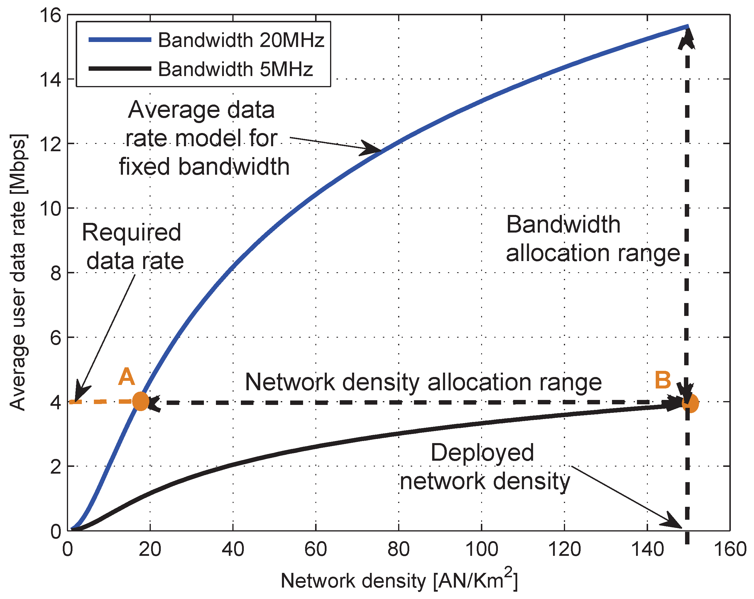
2.2. User Capacity in Dense Networks

We consider the downlink (DL) of a radio communication system with a network deployment, where the spatial location of ANs and active users in the network follows an homogeneous Poisson Point Process (PPP) with density ${\lambda }_b$ and ${\lambda }_u$, respectively. It has to be noted that PPPs possess the property of complete spatial randomness serving as reference when summary statistics are studied. In [16] it is shown that the locations of all cellular BSs in an area of 2.5 km × 2 km in a central park of London exhibit a rather random location than a nice deterministic pattern. In general, homogeneous PPP models permit statements about entire classes of wireless networks, and in particular UDNs. We also assume a path-loss attenuation with a distance dependent decay exponent $\alpha >2$ and users associated with the closest AN, so that the boundaries of the ANs coverage areas form a two-dimensional Voronoi tessellation. More specifically, users are connected to the AN providing the maximum reference signal received power (RSRP), e.g., as in the Long-Term Evolution (LTE) system. ANs with users in their coverage area transmit with fixed (unitary) power or are turned off otherwise. Under these assumptions, the ergodic user capacity per spectrum unit can be expressed as

$$\begin{array}{c}\hfill c({\lambda }_b,\alpha )=\mathbb{E}[\ln (1+SINR)][\mathrm{nats}/\mathrm{s}/\mathrm{Hz}],\end{array}$$

(1)

where the average is taken over the spatial distribution of the AN deployment and the distribution of the fading channel [13] Theorem 3. When ANs are distributed according to a Poisson Point Process with density ${\lambda }_b$, it was proven in [13] that for an interference-limited system (thermal noise power neglected) with interference following an exponential distribution (i.e., interference experiences only Rayleigh fading with no shadowing), the average ergodic capacity of the typical user becomes independent on the AN density ${\lambda }_b$ as

$$\begin{array}{c}\hfill c({\lambda }_b,\alpha )\equiv c(\alpha )=\underset{0}{\overset{\infty }{\int }}\frac{1}{1+{\rho }_t{(e^t-1)}^{2/\alpha }}\mathrm{d}t,\end{array}$$

(2)

where ${\rho }_t$ is a constant defined as ${\rho }_t={\int }_{{(e^t-1)}^{-2/\alpha }}^{\infty }\frac{1}{1+u^{\alpha /2}}\mathrm{d}u$. For instance, for $\alpha =4$, $c({\lambda }_b,\alpha )\approx$ 1.49 nats/s/Hz regardless of the AN density. This result proves that the overall sum throughput and area spectral efficiency of the network increase linearly with the AN density, since the number of users per area achieving c is exactly ${\lambda }_b$, assuming that the user density ${\lambda }_u$ is sufficiently large such that there is at least one user per cell.

Leveraging on these results from [13], Park et al. [17] have analyzed the asymptotic behavior of UDNs where the AN density is expected to be larger than the user density, i.e., ${\lambda }_b>>{\lambda }_u$, thereby resulting in ANs being switched off when not serving any user in their coverage area. In particular, by combining the results in [2] Proposition 1 with [13] Theorem 3, Equation (2) can be rewritten as

$$\begin{array}{c}\hfill c({\lambda }_b,{\lambda }_u,\alpha )=\underset{0}{\overset{\infty }{\int }}\frac{1}{1+{\rho }_t{(e^t-1)}^{2/\alpha }(1-p_{\mathrm{off}}({\lambda }_b,{\lambda }_u))}\mathrm{d}t,\end{array}$$

(3)

where $p_{\mathrm{off}}({\lambda }_b,{\lambda }_u)$ denotes the probability of an AN being turned off as a function of the AN density ${\lambda }_b$. Assuming that also the user location is distributed according to a Poisson Point Process with density ${\lambda }_b$, the probability p is approximated as (cf. [2] Proposition 1)

$$\begin{array}{c}\hfill p_{\mathrm{off}}({\lambda }_b,{\lambda }_u)={\left(1+\frac{{\lambda }_u}{3.5{\lambda }_b}\right)}^{-3.5}.\end{array}$$

(4)

The result in Equation (4) follows from the probability density function of the size of a typical Voronoi cell $f_X(x)=\frac{{3.5}^{3.5}}{\mathsf{\Gamma }(3.5)}{x}^{2.5}{e}^{-2.5x}$, where X denotes the size of the typical Voronoi cell normalized by $1/{\lambda }_b$, and $\mathsf{\Gamma }(·)$ is a Gamma function, derided in [18] through the Monte Carlo method.

On the other hand, for a regular grid of cells and users uniformly distributed, the probability of a cell being inactive and switched off becomes

$$\begin{array}{c}\hfill p_{\mathrm{off}}({\lambda }_b,{\lambda }_u)={\left(1+\frac{1}{{\lambda }_b}\right)}^{{\lambda }_u},\end{array}$$

(5)

where ${\lambda }_b\ge 1$ indicates the number of deployed ANs and ${\lambda }_u$ the number of users.

Based on Equations (3) and (4) and by defining ${\rho }_0={\int }_0^{\infty }\frac{1}{1+u^{\alpha /2}}\mathrm{d}u$, the following approximation for the average ergodic capacity of the typical user in UDNs is proposed in [17]

$$\begin{array}{c}\hfill c({\lambda }_b,{\lambda }_u,\alpha )\approx \log \left(1+{\left(\frac{{\lambda }_b}{{\rho }_0{\lambda }_u}\right)}^{\alpha /2}\right),{\lambda }_b>>{\lambda }_u.\end{array}$$

(6)

where Equation (6) supposedly approximates Equation (2) for ${\lambda }_b>>{\lambda }_u$. The above approximation can equivalently be based on Equations (3) and (5) since a regular grid of ANs is a special case of spatial randomness.

It must be noted that Equation (1) is not averaged over the multiple access of users (e.g., scheduling at the base station) and therefore represents the user spectral efficiency, not the user rate. Hence, the analysis of the average Ergodic user capacity implicitly assumes that each base station can serve all users in its coverage area with at least 1Hz of spectrum. To account for the multiple access of users with a fixed amount of spectrum, we shall next consider that each base station serves at least one user 1 Hz at any given time selected according to a uniform randomly scheduler. The average Ergodic user rate with uniformly random scheduler can be derived based on the user spectral efficiency $c({\lambda }_b,{\lambda }_b,\alpha )$, the fraction of BSs a user may access ${\lambda }_b/{\lambda }_u$, and the probability of an AN being in ON state $1-p_{\mathrm{off}}$ from Equation (5), as follows

$$\begin{array}{c}\hfill \begin{array}{c}r\left({\lambda }_b,{\lambda }_u,\alpha \right)=\left(1-p_{\mathrm{off}}\right)\frac{{\lambda }_b}{{\lambda }_u}c\left({\lambda }_b,{\lambda }_u,\alpha \right)\approx \frac{{\lambda }_u}{{\lambda }_b}\frac{{\lambda }_b}{{\lambda }_u}c\left({\lambda }_b,{\lambda }_u,\alpha \right)=c\left({\lambda }_b,{\lambda }_u,\alpha \right)\hfill \end{array}\end{array}$$

(7)

where $1-p_{\mathrm{off}}=1-{\left(1+1/{\lambda }_b\right)}^{{\lambda }_u}\approx {\lambda }_u/{\lambda }_b$, as derived in [19], and $c\left({\lambda }_b,{\lambda }_u,\alpha \right)$ is the user capacity approximation of Equation (6). This approximation of the multiple access, which suggests that in the ultra-dense network regime (i.e., ${\lambda }_b>>{\lambda }_u$) the multiple access of users can be simplified assuming that there is on average at most one user served per AN, yields a concave rate function for ${\lambda }_b>>{\lambda }_u$, which conveniently allows to formulate convex problems (cf. [17]).

2.3. Traffic Model

In this section, we describe traffic models that characterize the time and spatial variation of the traffic intensity demand in UDNs. To that end, we first describe traffic models developed by the EARTH project [20] to capture temporal variations of the traffic demand of a radio access network over a day. Then we extend these models to capture spatial correlation of the traffic demand in a geographical area by defining a traffic intensity map.

2.3.1. Long-Term Large-Scale Traffic Model

The EARTH project [20] has developed traffic models to determine the average served traffic on a certain time of the day in a given deployment scenario. By abstracting the models from the current cell planning maps in Europe, the methodology proposed by the EARTH project allows to deduce the daily variations as the actual traffic demand in a given area through the following steps:

• Define the average served data rates per user;
• Define the percentage of active users;
• Derive the deployment-specific peak data rate per unit area (Mbps/km${}^2$), given the population densities of the respective deployment scenario;
• Determine the deployment-specific data rates per unit area for a given time of the day with the aid of a daily traffic profiles.

(1) Data rate per user: The EARTH project has defined three traffic intensity profiles, or traffic profiles for simplicity, which correspond to different volumes of data rates generated by the users:

• High traffic intensity profile: 2.0 Mbps/user;
• Medium traffic intensity profile: 0.5 Mbps/user;
• Low traffic intensity profile: 0.1 Mbps/user.

(2) Percentage of active users: The percentage of the data subscribers active in the busy/peak hours in 2010 was roughly 10–30%, with an expected growth the ratio of broadband data subscribers of the whole population that by 2018 may exceed $25\%$ in the most mature European markets; however, conservative expectations calculate with $10\%$ as European average. The recommended aggregate reference values by the EARTH project are as follows:

• Percentage of radio broadband data subscribers: $10\%$ of the whole population;
• Percentage of active users in busy/peak hours: $20\%$ of the users;

Therefore, the number of active users amount to $2\%$ of the whole population in the busy/peak hours, which corresponds to roughly 10 users with active data connection in a typical 4G urban cell.

(3) Peak data rates in busy hours: As the data volume per subscriber does not depend on the deployment scenario, the normalized traffic values in

Table 1. EARTH traffic model for data traffic peaks in busy hours for different deployment scenarios.

Deployment	Population Density (citizens/Km${}^2$)	Traffic Profile (Mbps/Km${}^2$)
		High	Medium	Low
Dense urban	3000	120.0	30.0	6.0
Urban	1000	40.0	10.0	2.0
Sub-urban	500	20.0	5.0	1.0
Rural	100	4.0	1.0	0.2

are proportional to the population density. Given the population densities, the traffic demand per subscriber (high, medium, or low) and the number of active subscribers, the peak traffic demand per km${}^2$ of the considered deployment scenarios are listed in Table 1.

(4) Data rates over 24 h: The EARTH project [20] found that the daily variation of the number of active users scales with the daily variation of the traffic. The same normalized traffic profile is assumed for all deployments. Consequently, is assumed that the number of active users is scaled to match the traffic variations, while the average rates per active user remain fixed.

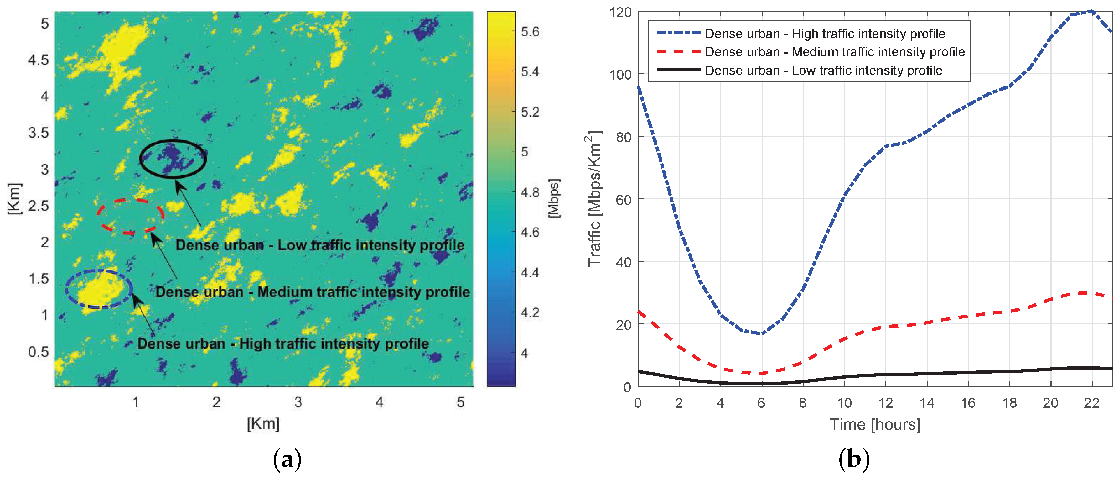
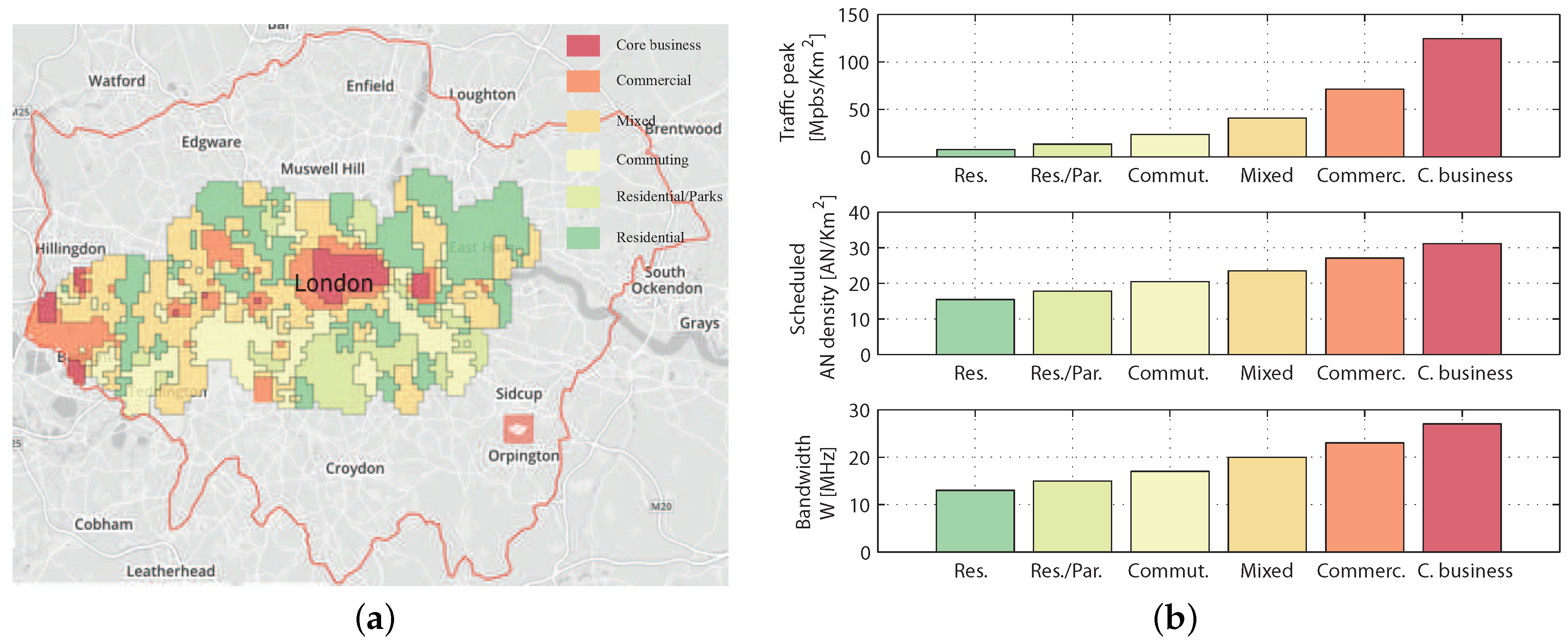
2.3.2. Traffic Intensity Maps

We extend the EARTH traffic models to capture the spatial variations of the traffic demand of the network deployment in Table 1. To that end, we assume a heterogeneous user behavior and, for a given time in the day, we create a traffic intensity map representing a temporal snapshot of the traffic intensity in a geographical area characterizing the spatial correlation of traffic.

A traffic intensity map is readily derived by multiplying a user density map with the estimated average user traffic peak reference value in the corresponding hour to which the traffic map refers to. We assume that active users in geographical region are log-normally distributed around a large-scale mean ${\lambda }_u$ and with a small-scale standard deviation ${\sigma }_u$ adjusted to achieve the peak values of the user distribution with a reasonable probability (cf. [21,22]).

Assuming that the density of active users ${\lambda }_u$ is scaled to match the traffic variations, while the average rates per active user remain fixed, the traffic density maps are created by multiplying the user densities and per-user traffic intensities. An example of a traffic map is showed in Figure 3a representing a temporal snapshot of a 5 km × 5 km dense urban deployment, where the traffic profiles ranges from high to low in different areas. Figure 3b shows the daily variations of the traffic peak for three areas with high, medium, and low traffic.

2.4. Traffic Constraints

For a given frequency bandwidth W, the two models of average user spectral efficiency and average user traffic demand can be combined into the following average user rate constraint

$$\begin{array}{c}\hfill t_u\le Wc({\lambda }_b,\alpha ).\end{array}$$

(8)

stating that the average user data rate supplied by the network (in the right-hand side) shall be grater or equal to the average user traffic demand $t_u$ (bps) (in the left-hand side). Thus, the density of the active ANs ${\lambda }_b$ and the associated frequency spectrum bandwidth W can be optimized to fulfill the average traffic demand of the users.

3. Joint Network Density and Frequency Spectrum Optimization

In this section, we exploit the models introduced in Section 2 to develop new radio resource management algorithms to schedule the density of active ANs and the frequency bandwidth required in an ultra-dense network to support a given user traffic demand. In particular, we develop RRM algorithms for two application scenarios: (a) in Section 3.1 we consider the resource management problem for network operator owning a dedicated pool of frequency resources; (b) in Section 3.2, we consider the resource management problem for multiple network operators with co-located network deployment sharing a common frequency pool of frequency resources.

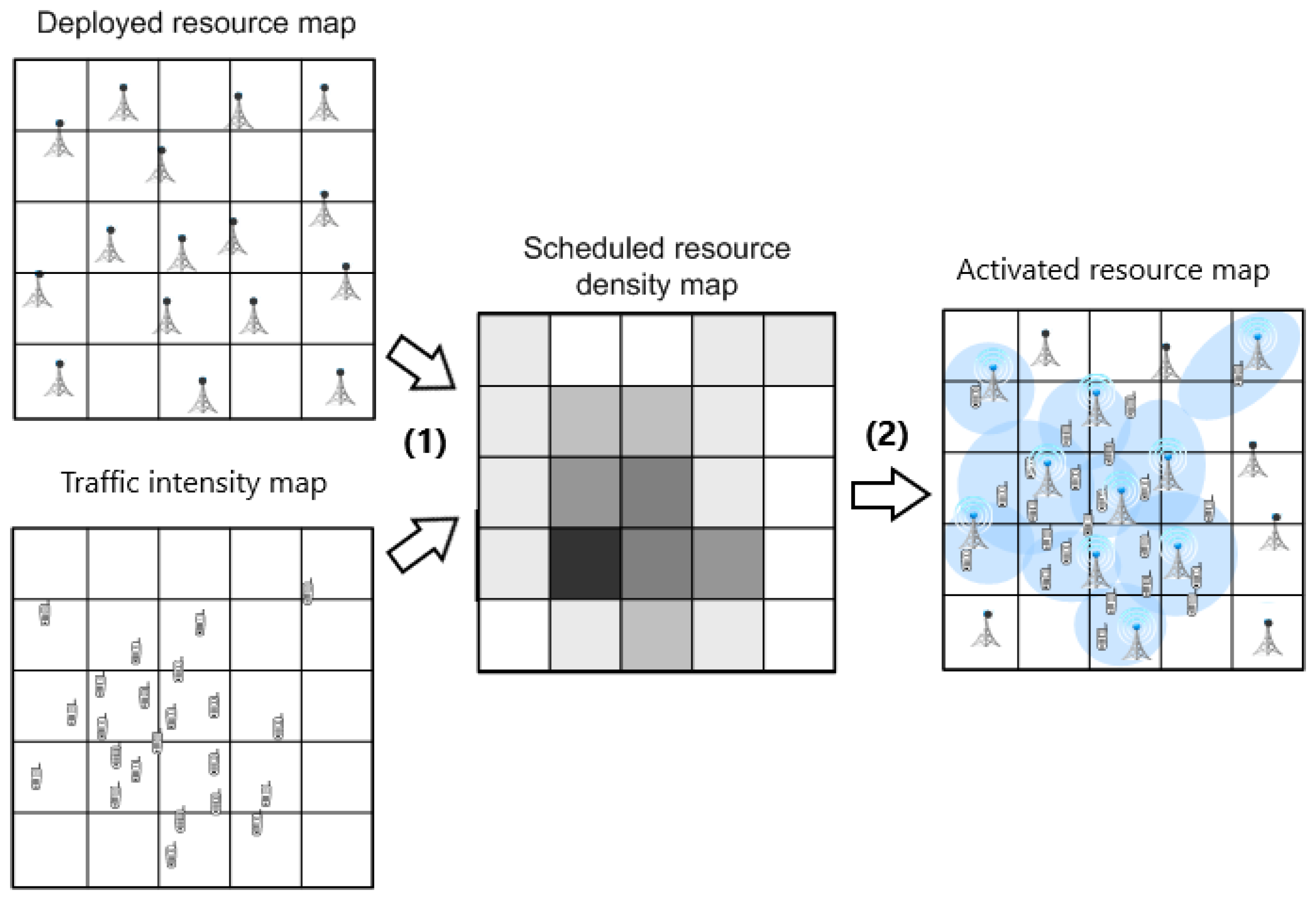
3.1. Network Density and Spectrum Scheduler

We consider a network deployment with deployed access node density ${\lambda }_{b,\max }$ (number of AN/Km${}^2$), density of active users ${\lambda }_u$ (number of UE/Km${}^2$), and maximum available bandwidth per access nodes $W_{\max }$. Using the traffic constraint Equation (8), we formulate a joint the network density and spectrum scheduling problem as

$$\begin{array}{c}\hfill \begin{array}{cc}{\displaystyle \mathrm{minimize}}\hfill & c_b{\lambda }_b+c_{w}W\hfill \\ \mathrm{subject}\mathrm{to}\hfill & t_u\le W\log \left(1+{\left(\frac{{\lambda }_b}{{\rho }_0{\lambda }_u}\right)}^{\frac{\alpha }{2}}\right)\hfill \\ & {\lambda }_b\le {\lambda }_{b,\max },W\le W_{\max },\hfill \end{array}\end{array}$$

(9)

where the optimization variables are the scheduled density of active ANs ${\lambda }_b$ and the allocated frequency bandwidth W. The objective of this problem is to minimize a network-wide cost function that depends on a cost $c_b$ associated with the network infrastructure and a cost $c_w$ associated with the use of frequency bandwidth. The values $c_b$ and $c_w$ can model network operational costs (e.g., the running cost of ANs and spectrum leasing), energy costs (e.g., the energy cost of ANs and spectrum), or other cost functions.

The outcome of the problem  (9) is the optimal density ${\lambda }_b^{\star }$ of active ANs and the optimal frequency bandwidth $W^{\star }$ that the system operator needs to use in a certain geographical region so as to meet the user traffic demand, as summarized by the following proposition.

Proposition 1.

Problem (9) is not jointly convex in the variables ${\lambda }_b$ and W. An equivalent convex formulation can be found through a variable transformation ${\lambda }_b\to e^{{\tilde{\lambda }}_b}$, $W\to e^{\tilde{W}}$ and a log-transformation of the constraint function, as follows

$$\begin{array}{c}\hfill \begin{array}{cc}\mathrm{minimize}\hfill & c_b{e}^{{\tilde{\lambda }}_b}+c_w{e}^{\tilde{W}}\hfill \\ \mathrm{subject}\mathrm{to}\hfill & \log (t_u)\le \tilde{W}+\log \left[\log \left(1+{\left(\frac{e^{{\tilde{\lambda }}_b}}{{\lambda }_u}\right)}^{\frac{\alpha }{2}}\right)\right]\hfill \\ & {\tilde{\lambda }}_b\le \log ({\lambda }_{b,\max }),\tilde{W}\le \log (W_{\max }).\hfill \end{array}\end{array}$$

(10)

Problem (10) admits a globally optimal solution that correspond to the global optimal solution of the original problem (9), which can be achieved through the distributed RRM Algorithm 1.

Proof. 

See Appendix A. □

The network resource density scheduler in Figure 1 is therefore implemented by an instance of Algorithm 1. In a subsequent step, the network resource scheduler determines the allocation of frequency resources (e.g., which resource blocks and which frequency band) to be used by the active AN, and will control the ON/OFF operation of ANs in the region so as to track local traffic changes in a fast time-scale, while maintaining the scheduled network density over a slower time-scale [4].

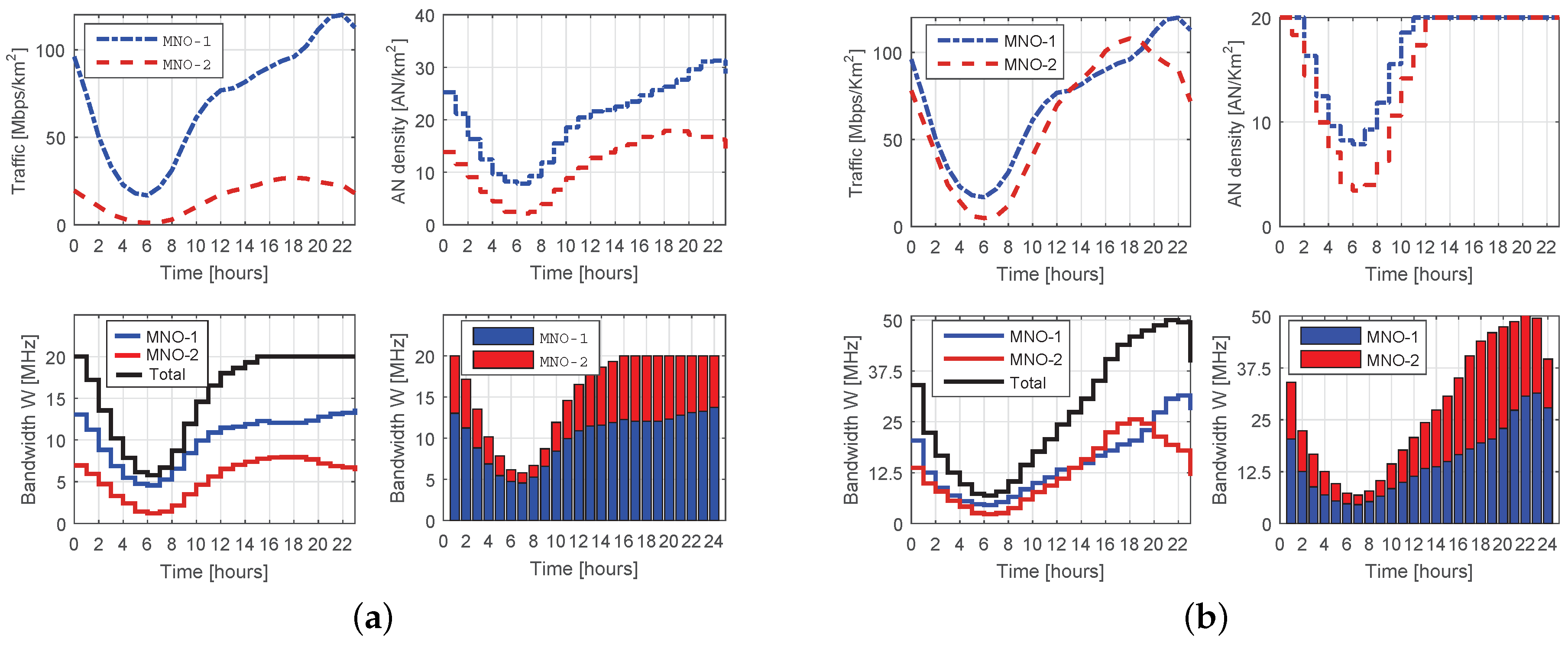
3.2. Multi-Operator Spectrum Sharing

The framework of Section 3.1 is herewith extended to the resource management problem associated with multi-operator spectrum sharing in UDNs. To that end, we hereafter consider $N>1$ operators with co-located network deployments in a geographical area with density ${\lambda }_{b,n}$ (number of AN/Km${}^2$), respectively, sharing a common pool of frequency bandwidth of size $W_{\max }$. We further assume that each operator has a user density ${\lambda }_{u,n}$ (number of UE/Km${}^2$) with average traffic density demand $t_{u,n}$ (bps/user). Under these assumptions, we consider two types of spectrum sharing scenarios based on: exclusive spectrum allocation where each operator is allocated a portion $W_n$ of the available frequency bandwidth $W_{\max }$ for exclusive use, hence ${\sum }_n{W}_n\le W_{\max }$; and non-exclusive spectrum allocation, where each operator is allocated a portion $W_n$ of the available frequency bandwidth $W_{\max }$ that may partly or fully overlap with the spectrum allocation of another operator. The objective of the problem in both scenarios is to minimize a network-wide cost function that depends on operators’ cost $c_{b,n}$ associated with the network infrastructure and a cost $c_{w,n}$ associated to the use of frequency bandwidth.

Algorithm 1 Jointly optimal frequency bandwidth and network density scheduler.

Initialize: $t=0$; ${\lambda }_b^{(0)}=\mathrm{const}.;$$W^{(0)}=\mathrm{const}.;$$ϵ$ sufficiently small constant. repeat   Update primal variable as: $$\begin{array}{ccc}\hfill {\lambda }_b^{(i)}& =& \min \left\{\frac{{\mu }^{(i-1)}}{c_1}\left[\frac{\alpha }{2}\frac{{\left(\frac{{\lambda }_b^{(i-1)}}{{\rho }_0{\lambda }_u}\right)}^{\frac{\alpha }{2}}}{1+{\left(\frac{{\lambda }_b^{(i-1)}}{{\rho }_0{\lambda }_u}\right)}^{\frac{\alpha }{2}}}\frac{1}{\log \left(1+{\left(\frac{{\lambda }_b^{(i-1)}}{{\rho }_0{\lambda }_u}\right)}^{\frac{\alpha }{2}}\right)}\right],{\lambda }_{b,\max }\right\},\hfill \end{array}$$ (11) $$\begin{array}{ccc}\hfill W^{(i)}& =& \min \left\{\frac{{\mu }^{(i-1)}}{c_2},W_{\max }\right\}\end{array}$$ (12)   Update dual variable as: $$\begin{array}{c}\hfill {\mu }^{(i)}={\left[{\mu }^{(i-1)}+ϵ\left(\log (t_u)\log \left(W^{(i)}\log \left(1+{\left(\frac{{\lambda }_b^{(i)}}{{\rho }_0{\lambda }_u}\right)}^{\frac{\alpha }{2}}\right)\right)\right)\right]}^{+},\end{array}$$ (13) until convergence.

3.2.1. Exclusive Spectrum Allocation

With exclusive spectrum allocation, problem (9) can be generalized to a joint network density and spectrum sharing problem to be solved by each operator as

$$\begin{array}{c}\hfill \begin{array}{ccc}{\displaystyle \mathrm{minimize}}\hfill & \sum _{n=1}^N{c}_{b,n}{\lambda }_{b,n}+c_{w,n}{W}_n\hfill & \\ {\displaystyle \mathrm{subject} \mathrm{to}}\hfill & t_{u,n}\le W_n\log \left(1+{\left(\frac{{\lambda }_{b,n}}{{\rho }_n{\lambda }_{u,n}}\right)}^{\frac{\alpha }{2}}\right)\hfill & n=1,\cdots ,N,\hfill \\ & \sum _{n=1}^N{W}_n\le W_{\max },\hfill & \\ & {\lambda }_{b,n}\le {\lambda }_{b,n,\max }\hfill & n=1,\cdots ,N,\hfill \end{array}\end{array}$$

(14)

where the optimization variables ${\lambda }_{b,n}$ and $W_n$ denote the network density and the fraction of bandwidth allocated to operator n, respectively. The first set of constraints represent the traffic demand per operator, while the inequality ${\sum }_{n=1}^N{W}_n\le W_{\max }$ assures an exclusive allocation of spectrum among the operators. The values $c_{b,n}$ and $c_{w,n}$ can model network operational costs (e.g., the running cost of ANs and spectrum leasing), energy costs (e.g., the energy cost of ANs and spectrum), or other cost functions.

The outcome of the problem (14) is the optimal density ${\lambda }_{b,n}^{\star }$ of active ANs and the optimal frequency bandwidth $W_n^{\star }$ that the network operator needs to use in a geographical region so as to meet region’s user traffic demand, as summarized by the following proposition.

Proposition 2.

Problem (14) is not jointly convex in the variables ${\lambda }_{b,n}$ and $W_n$. An equivalent convex formulation can be found through a variable transformation ${\lambda }_{b,n}\to e^{{\tilde{\lambda }}_{b,n}}$, $W_n\to e^{\widetilde{W_n}}$ and a log-transformation of the constraint function, as follows

$$\begin{array}{c}\hfill \begin{array}{ccc}{\displaystyle \mathrm{minimize}}\hfill & \sum _{n=1}^N{c}_{b,n}{e}^{{\tilde{\lambda }}_{b,n}}+c_{w,n}{e}^{{\tilde{W}}_n}\hfill & \\ {\displaystyle \mathrm{subject} \mathrm{to}}\hfill & \log (t_{u,n})\le {\tilde{W}}_n+\log \left[\log \left(1+{\left(\frac{e^{{\tilde{\lambda }}_{b,n}}}{{\rho }_n{\lambda }_{u,n}}\right)}^{\frac{\alpha }{2}}\right)\right]\hfill & \forall n,\hfill \\ & \log \left(\sum _{n=1}^N{e}^{{\tilde{W}}_n}\right)\le \log (W_{\max }),\hfill & \\ & {\tilde{\lambda }}_{b,n}\le \log ({\lambda }_{b,n,\max })\hfill & \forall n.\hfill \end{array}\end{array}$$

(15)

Problem (15) admits a globally optimal solution that correspond to the global optimal solution of the original problem (14), which can be achieved through the distributed RRM Algorithm 2.

Proof. 

See Appendix A. □

Algorithm 2 Jointly network density and spectrum sharing.

Initialize: $t=0$; ${\lambda }_{b,n}^{(0)}=\mathrm{const}.;$$W_n^{(0)}=\mathrm{const}.;$${\rho }_n=\mathrm{const}.;$$ϵ$ sufficiently small constant. repeat   Update primal variable as: $${\lambda }_{b,n}^{(i)}=\min \left\{\frac{{\mu }_n^{(i-1)}}{c_{b,n}}\left[\frac{\alpha }{2}\frac{{\left(\frac{{\lambda }_{b,n}^{(i-1)}}{{\rho }_n{\lambda }_{u,n}}\right)}^{\frac{\alpha }{2}}}{1+{\left(\frac{{\lambda }_{b,n}^{(i-1)}}{{\rho }_n{\lambda }_{u,n}}\right)}^{\frac{\alpha }{2}}}\frac{1}{\log \left(1+{\left(\frac{{\lambda }_{b,n}^{(i-1)}}{{\rho }_n{\lambda }_{u,n}}\right)}^{\frac{\alpha }{2}}\right)}\right],{\lambda }_{b,\max }\right\},$$ (16) $$W_n^{(i)}=\min \left\{\frac{{\mu }_n^{(i-1)}}{c_{w,n}+{\omega }^{(i-1)}{\sum }_{j=1}^N{W}_j^{(i-1)}},W_{\max }\right\}$$ (17)   Update dual variable as: $${\mu }_n^{(i)}={\left[{\mu }_n^{(i-1)}+ϵ\left(\log (t_{u,n})-\log \left(W_n^{(i)}\log \left(1+{\left(\frac{{\lambda }_{b,n}^{(i)}}{{\rho }_n{\lambda }_{u,n}}\right)}^{\frac{\alpha }{2}}\right)\right)\right)\right]}^{+},$$ (18) $${\omega }^{(i)}={\left[{\omega }^{(i-1)}+ϵ\left(\log \left(\sum _{n=1}^N{W}_n^{(i)}\right)-\log (W_{\max })\right)\right]}^{+}.$$ (19) until convergence.

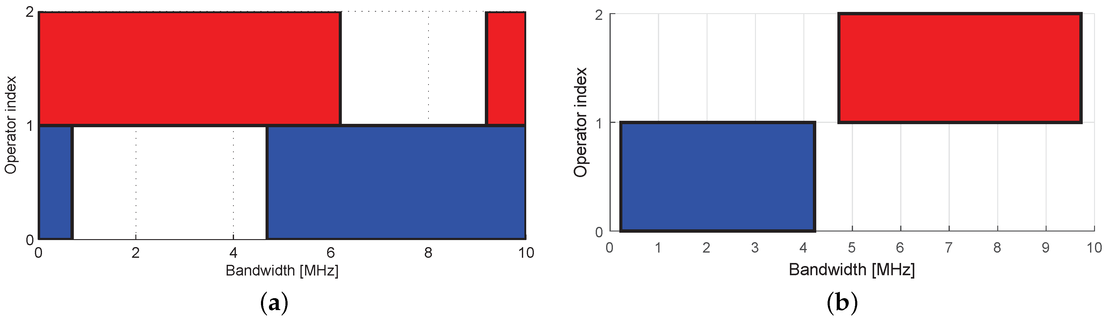
3.2.2. Non-Exclusive Spectrum Allocation

To capture non-exclusive spectrum allocation among different operators we introduce the variables $W_{n,n}$ and $W_{n,j}$ indicating the fraction of the frequency bandwidth $W_n$ that an operator n is allocated in exclusive and non-exclusive manner with respect to a second operator j, respectively, as well as the variables $t_{n,n}$ and $t_{n,j}$ indicating the fraction of the traffic density $t_{u,n}$ of operator n served within $W_{n,n}$ and $W_{n,j}$, respectively.

Thus, we formulate the multi-operator network density and frequency spectrum scheduling with non-exclusive spectrum allocation for the case of two operators as

$$\begin{array}{c}\hfill \begin{array}{ccc}{\displaystyle \mathrm{minimize}}\hfill & \sum _{n=1}^2{c}_{b,n}{\lambda }_{b,n}+c_{w,n}{W}_n\hfill & \\ \mathrm{subject}\mathrm{to}\hfill & t_{n,n}\le W_{n,n}\log \left(1+{\left(\frac{{\lambda }_{b,n}}{{\lambda }_{u,n}}\right)}^{\frac{\alpha }{2}}\right)\hfill & n=1,2,\hfill \\ & t_{n,j}\le W_{n,j}\log \left(1+{\left(\frac{{\lambda }_{b,n}}{{\lambda }_{u,n}}\right)}^{\frac{\alpha }{2}}\right)\hfill & n,j=1,2,j\ne n,\hfill \\ & \sum _{j=1}^2{t}_{n,j}\le t_{u,n}\hfill & n=1,2,\hfill \\ & \sum _{j=1}^2{W}_{n,j}=W_n\hfill & n=1,2,\hfill \\ & W_{1,2}=W_{2,1},\hfill & \\ & {\lambda }_{b,n}\le {\lambda }_{b,n,\max }\hfill & n=1,2,\hfill \end{array}\end{array}$$

(20)

where the variables ${\lambda }_{b,n}$ and $W_n$ denote the network density and the fraction of bandwidth scheduled for operator i, respectively. The first set of inequalities relates a portion of traffic to spectrum allocated for exclusive use to each operator, while the second set of inequalities relates the remaining portion of traffic of each operator to shared spectrum. In problem (20), the portion of traffic that each operator serves with spectrum allocated for exclusive and non-exclusive are additional optimization variables, whose sum is bounded by the total traffic demand of the operator.

Similarly to problem (9), the first set of constraints represent the traffic demand per operator, while the inequality ${\sum }_{n=1}^N{W}_n\le W_{\max }$ assures an orthogonal allocation of spectrum to the various operators within the frequency bandwidth $W_{\max }$.

Similar to previous formulations, the problem (20) is not a convex optimization. However, an equivalent convex formulation can be found through the variable transformation $x\to e^{\tilde{x}}$, and a log-transformation of the constraints as follows

$$\begin{array}{c}\hfill \begin{array}{ccc}{\displaystyle \mathrm{minimize}}\hfill & \sum _{n=1}^2{c}_{b,n}{e}^{{\tilde{\lambda }}_{b,n}}+c_{n,w}{e}^{{\tilde{W}}_n}\hfill & \\ \mathrm{subject}\mathrm{to}\hfill & \log (t_{b,n})\le {\tilde{W}}_{n,n}+\log \left[\log \left(1+{\left(\frac{e^{{\tilde{\lambda }}_{b,n}}}{{\lambda }_{u,n}}\right)}^{\frac{\alpha }{2}}\right)\right]\hfill & n=1,2,\hfill \\ & \log (e^{{\tilde{t}}_{n,j}})\le {\tilde{W}}_{n,j}+\log \left[\log \left(1+{\left(\frac{e^{{\tilde{\lambda }}_{b,n}}}{{\lambda }_{u,n}}\right)}^{\frac{\alpha }{2}}\right)\right]\hfill & n,j=1,2,j\ne n\hfill \\ & \log (\sum _{j=1}^2{e}^{{\tilde{t}}_{n,j}})\le \log (t_{u,n})\hfill & n=1,2,\hfill \\ & \log (\sum _{j=1}^2{e}^{{\tilde{W}}_{n,j}})\le {\tilde{W}}_n,\hfill & n=1,2,\hfill \\ & {\tilde{W}}_{1,2}={\tilde{W}}_{2,1},\hfill \\ & {\tilde{\lambda }}_{b,n}\le \log ({\lambda }_{b,n,\max })\hfill & n=1,2.\hfill \end{array}\end{array}$$

(21)

Thus, the global optimal solution to the spectrum sharing problem (20) can be found by solving problem (21).

3.2.3. Frequency Spectrum Location

In the previous subsection, we derived two different schemes, an exclusive and a non-exclusive, for the allocation of the density of active ANs and the frequency bandwidth. These schemes target UDNs in the case of multiple system operators with network deployments co-located in the same geographical area sharing a common frequency pool of frequency spectrum resources. In this section, we will address how to determine the exact allocation of frequency bands among the operators based on the frequency bandwidth derived by the global optimum. The frequency bandwidth derived by solving the optimization problem corresponds to the amount of frequency resources $W_n$ an operator, n, may request to meet the traffic demands on its network from a total frequency bandwidth $W_{max}$.

The exact allocation of frequency bands requires a sorting function, $\zeta$, that defines an order among the operators, for instance, based on the operators’ requested bandwidth, $W_1,W_2,\cdots ,W_N$. The sorting is a permutation (a reordering) of the values $W_1,W_2,\dots ,W_N$ (e.g., ascending or descending). To this end, we let $W_i$ be the requested bandwidth of operator i, and let $\zeta$ be any permutation of the set $W_1,W_2,\dots ,W_N$ such that

$$\begin{array}{c}\hfill W_{\zeta (1)}\ge \cdots \ge W_{\zeta (N)}.\end{array}$$

(22)

For example, operators can be sorted in ascending or descending order of their frequency spectrum demand, in a predefined order, etc. Ties are broken by applying multiple ordering criteria, for instance, frequency spectrum demand followed by network identifier order. The sorting criteria used by the sorting function, $\zeta (i)$, constitute a kind of an etiquette operation protocol. The output of the sorting function is used to further assign an operator to portions of the frequency pool. Following the order of the operators as determined by $W_{\zeta (i)}$ the allocation of the spectrum interval $[{\phi }_{\zeta (i)}^{begin},{\phi }_{\zeta (i)}^{end}]$ for the ith operator can be iteratively derived by Algorithm 3. The variables ${\phi }_{\zeta (i)}^{begin}$, ${\phi }_{\zeta (i)}^{center}$, and ${\phi }_{\zeta (i)}^{end}$ denote the starting, center and ending frequency of the spectrum interval of the ith operator respectively and with ${\phi }_{\zeta (0)}^{end}=0$. The ith iteration step concludes with a frequency spectrum wrap-around for those intervals exceeding the boundaries of the spectrum bandwidth i.e., ${\phi }_{\zeta (i)}^{begin}<0$ and ${\phi }_{\zeta (i)}^{end}>W$ then spectrum intervals are adjusted by ${\phi }_{\zeta (i)}^{begin}=W_{\max }+{\phi }_{\zeta (i)}^{begin}$ and ${\phi }_{\zeta (i)}^{end}={\phi }_{\zeta (i)}^{end}-W_{max}$ respectively.

Algorithm 3 Resource scheduling of frequency spectrum.

Find a permutation $\zeta$ on the set of operators’ requested bandwidth $W_1,W_2,\dots ,W_N$ such that $W_{\zeta (1)}\ge \cdots \ge W_{\zeta (N)}$ Initialize: $i=0$, ${\phi }_{\zeta (0)}^{end}=0$. repeat   $i=i+1$   Compute the location of the spectrum band as: $$\begin{array}{c}\hfill {\phi }_{\zeta (i)}^{center}={\phi }_{\zeta (i-1)}^{end}+\frac{W_{\zeta (i)}{W}_{max}}{2{\sum }_{j=1}^N{W}_j},\\ \hfill {\phi }_{\zeta (i)}^{begin}={\phi }_{\zeta (i)}^{center}-\frac{W_{\zeta (i)}}{2},\\ \hfill {\phi }_{\zeta (i)}^{end}={\phi }_{\zeta (i-1)}^{center}+\frac{W_{\zeta (i)}}{2}\end{array}$$ (23)   if ${\phi }_{\zeta (i)}^{begin}<0$ then    ${\phi }_{\zeta (i)}^{begin}=W_{max}+{\phi }_{\zeta (i)}^{begin}$   else if ${\phi }_{\zeta (i)}^{end}>W_{max}$ then    ${\phi }_{\zeta (i)}^{end}={\phi }_{\zeta (i)}^{end}-W_{max}$   end if until i==N.

Figure 4 illustrate two examples of this method. Figure 4a illustrates an example with non-exclusive spectrum use allocated in a descending order of demand, while Figure 4b illustrates an example with exclusive spectrum use allocated in ascending order of demand where the system operators share the spectrum according to their spectrum request. The spectrum allocation in Figure 4 is therefore implemented by an instance of Algorithm 3, which can be performed in a centralized manner, by a control entity, or a distributed manner, by each operator independently, assuming that operators exchange their frequency bandwidth demands.

4. Numerical Results

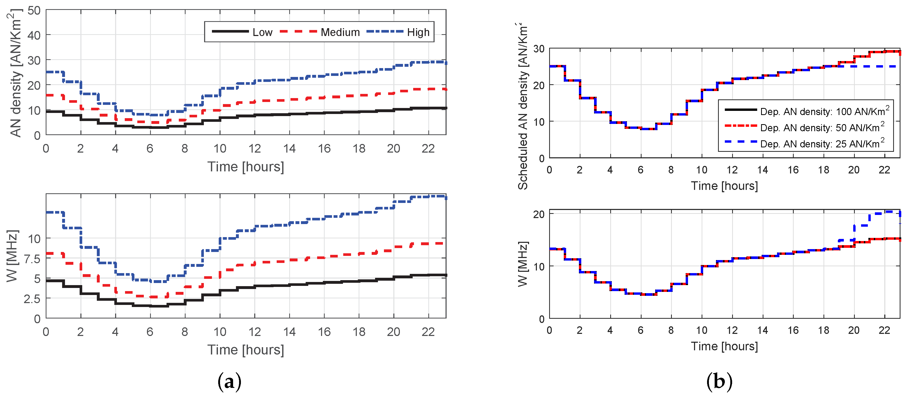
4.1. Network Density and Frequency Bandwidth Optimization

In this section, we present some illustrative results of Algorithm 1 when it is used to jointly optimize the allocation of frequency spectrum bandwidth and the density of active ANs over a day. The algorithm effectively implements a network density scheduler which optimization goal is to minimize a network cost function (e.g., the network operational cost or the energy cost) while providing a requested average peak traffic demand of active users. An illustration of the devised solution is given in Figure 5 depicting two MNOs, where the density scheduler of each MNO optimizes the density of active ANs and their allocation of frequency bandwidth. In this example, the network scheduler of the first operator “MNO-1” optimizes for each three geographical sub-regions, labeled 1.1 to 1.3, of the network to meet the corresponding traffic intensity demands. In similar manner operates the network scheduler of the second operator “MNO-2” for the three geographical sub-regions, labeled 2.1 to 2.3, under its control. Assuming the same cost function is used for all regions, the region with lower traffic demand is allocated less frequency bandwidth and scheduled to use a smaller density of active ANs. In each region, ANs are dynamically switched ON/OFF to follow fast and local variations in user mobility and traffic demand, while keeping the overall density of scheduled ANs constant. It should be noted that while the scheduled frequency bandwidth and AN density are adapted on a relatively slow time-scales (tens of minutes to hours) by the density scheduler (cf. Figure 1), the ANs in a region of the system are dynamically switched ON/OFF on a faster time-scale by a resource scheduler (cf. Figure 6b) to track local variations in user mobility and traffic demand while keeping the overall density of scheduled ANs constant.

Figure 6 illustrates how the network resource density scheduler can track long-term large-scale changes in the average traffic demand over time. To this end, we resort to traffic models proposed by the EARTH project [20] (cf. Section 2.3) which characterize the variation of the traffic intensity in time domain (e.g., one day variation) for various deployment scenarios. The numerical results follow the typical 1-day traffic intensity profile (Mbps/Km${}^2$) of a dense urban area with high (in blue dash-dotted line), medium (in red dashed line),and low (in black solid line) traffic profiles as shown in Figure 3b. The network deployment in a dense urban area corresponds to a population density of 3000 citizens/Km${}^2$. Given the population density, the traffic demand per subscriber (high, medium or low), the number of active subscribers corresponding to $2\%$ of the population density, and the peak traffic demand per km${}^2$ of the urban dense deployment, as listed in Table 1, the traffic profile over 24 h is calculated as a percentage of the traffic peak (with traffic peak corresponding to $100\%$).

The two plots of Figure 6a illustrates the scheduled access node density (AN/Km${}^2$) (upper plot) and frequency spectrum bandwidth (MHz) (lower plot), respectively, required to meet the traffic intensity demand at each hour of the day. In this example, we assume that the system operator has available a bandwidth $W_{\max }$ = 20 MHz and deployed a network with access nodes density ${\lambda }_{b,dep}$ = 50 AN/Km${}^2$ (corresponding to roughly 140 m inter-site distance). The path-loss attenuation between an AN and a user is modeled with a distance dependent decay exponent of $\alpha =4$. In hours of light traffic intensity, the scheduled AN density and the scheduled bandwidth are both within the deployed resource limits. When the traffic intensity exceeds a certain value (e.g., at 12 a.m. for high traffic profile in this example), the full bandwidth is $W_{\max }$ is allocated to active access points, and further increases in traffic intensity demand are compensated by increasing the scheduled network density.

Figure 6b analyzes the impact of the deployed network density by considering an dense urban scenario with high traffic profile and three network deployments with uniform distribution of ANs with average inter-site distance of ISD${}^{(1)}=250$ m, ISD${}^{(2)}=140$ m, and ISD${}^{(3)}=100$ m, respectively, corresponding to deployed network densities of ${\lambda }_{b,dep}^{(1)}=25$ AN/Km${}^2$, ${\lambda }_{b,dep}^{(2)}=50$ AN/Km${}^2$, ${\lambda }_{b,dep}^{(3)}=100$ AN/Km${}^2$, respectively. In this example, we assume that the system operator has available a sufficiently large bandwidth $W_{\max }$ = 100 MHz so that the limiting factor in the optimization is the deployed network density. The results show that, beyond a certain traffic intensity, the sparser network deployment requires hours with high traffic load to be fully used, and an increase traffic demand is compensated by scheduling more frequency bandwidth. Denser network deployments, on the other hand, are characterized by the same allocation of resources as the deployed resource limits are never fully used.

The traffic models of EARTH project [20] have been further extended to capture spatial variation of traffic through the definition of traffic intensity maps (cf. Section 2.3). A traffic intensity map is therefore a temporal snapshot of the traffic intensity in a geographical area characterizing the spatial correlation of traffic. The combination of traffic intensity maps and the typical time profile of the traffic peak demand of the EARTH project [20] yields a full characterization of the traffic intensity in space and time. Figure 7a illustrates and example of traffic intensity map for a metropolitan area. The city area is divided into clusters, each characterized by a different traffic intensity as listed in the top most plot of Figure 7b. In this example, we have generated the traffic intensity of each cluster through the model in Section 2.3, by partitioning the traffic intensity map of Figure 3a into six clusters of different traffic intensity, and associating each traffic intensity to each cluster of Figure 7a. It must be noted that the association of the traffic intensity to the cluster types of Figure 7a is arbitrary. The ordering of traffic intensity, as well as the traffic intensity values, may change at different time of the day. For this simulation setup, Figure 7b shows the scheduled access node density (AN/Km${}^2$) and frequency spectrum bandwidth (MHz) required to meet the traffic intensity demand of each cluster assuming that the system operator has available a bandwidth $W_{\max }$ = 50 MHz and deployed a radio access network with AN density ${\lambda }_{b,dep}=50$ AN/Km${}^2$ throughout the city area.

4.2. Network Density and Spectrum Sharing Optimization

The proposed joint network density and spectrum sharing Algorithm 2 is evaluated by means of simulations for an example scenario of $N=2$ RAN operators of co-located (but not shared) UDN deployments (cf. [20]) sharing a common pool of frequency resources (cf. Section 3.2). The general framework, which is given in [4], allows for an implementation of the algorithm in either a centralized fashion, with a resource density scheduler acting as a spectrum manager that determines the allocation of frequency spectrum for different network operators, or a distributed fashion, with network density schedulers of different operators coordinating to determine the optimal allocation of frequency spectrum and AN density for a certain geographical area. The latter is also illustrated in Figure 5.

Based on the same traffic, network deployment and path-loss assumptions as for a single operator’s network density and frequency bandwidth optimization, Figure 8 shows a numerical example of joint network density scheduling and spectrum sharing for two network operators with co-located (but not shared) RAN deployments in a dense urban area (cf. [20]) sharing a bandwidth $W_{\max }=20$ MHz. In particular, it shows the simulation results for two different density deployments and spectrum sharing scenarios with different traffic mixtures [14]. The upper left plots of Figure 8a,b show the typical time profile of the traffic demand (in (Mbps/km${}^2$)) for each operator over a day, the upper right plots depict the corresponding scheduled network densities (in (AN/km${}^2$)) for each network operator, while the lower left plots show the corresponding frequency bandwidth (in (MHz)) allocated to each operator. Finally, the lower right plots of Figure 8a,b illustrate how the available frequency bandwidth $W_{\max }$ can be split among the two system operators based on the allocation of the distributed RRM Algorithm 2. Figure 8a illustrates a scenario of an operator with high traffic profile “MNO-1” and an operator with medium traffic profile “MNO-2” in a dense urban area sharing a bandwidth that is restricted to $W_{\max }$ = 20 MHz. In Figure 8b each operator employs a high traffic profile and a UDN density of 20 AN/km${}^2$. It can be noticed that when the cumulative peak traffic is sufficiently low, a portion of the available frequency bandwidth remains unallocated to any operator, while in hours of the day when the cumulative peak traffic exceeds a certain value, the entire frequency bandwidth is split among the two system operators. In the peak/busy hours, the proposed algorithm provides higher spectral efficiency by scheduling higher density of ANs to be used by each system operator.

5. Conclusions

In this research work we have exploited a network optimization problem where the allocation of spectrum bandwidth and the density of active ANs are jointly optimized to minimize a network operational cost, and we have used Lagrange duality techniques to develop provably optimal RRM algorithms. The new RRM algorithms have been applied and evaluated on two application scenarios: (a) the resource management problem for an operator of an ultra-dense network with exclusive access to a pool of frequency resource; and (b) the resource management problem for multiple operators of co-located UDNs sharing a common pool of frequency resources. The feasibility of the algorithms’ joint network density and spectrum sharing approach for adapting the spectrum and network resources to operators’ traffic load over the duration of a day has been demonstrated by means of simulations.

References

1. Andrews, J.G.; Buzzi, S.; Choi, W.; Hanly, S.V.; Lozano, A.; Soong, A.C.K.; Zhang, J.G. What will 5G be? IEEE J. Sel. Areas Commun. 2014, 32, 1065–1082. [Google Scholar] [CrossRef]
2. Yu, A.M.; Kim, S.L. Downlink capacity and base station density in cellular networks. In Proceedings of the IEEE WiOpt Workshop on Spatial Stochastic Models for Wireless Networks, Tsukuba, Japan, 13–17 May 2013. [Google Scholar]
3. Galiotto, C.; Marchetti, N.; Doyle, L. The role of total transmit power on the linear area spectral efficiency gain of cell splitting. IEEE Commun. Lett. 2013, 17, 2256–2259. [Google Scholar] [CrossRef]
4. Koudouridis, G.P.; Soldati, P. Spectrum and Network Density Management in 5G Ultra-Dense Networks. IEEE Wirel. Commun. 2017, 24, 30–37. [Google Scholar] [CrossRef]
5. Hadzialic, M.; Dosenovic, B.; Dzaferagic, M.; Musovic, J. Cloud-RAN: Innovative Radio Access Network Architecture. In Proceedings of the Electronics in Marine-2013, Zadar, Croatia, 25–27 September 2013; pp. 115–120. [Google Scholar]
6. Eramo, V.; Listanti, M.; Lavacca, F.G.; Iovanna, P.; Bottari, G.; Ponzini, F. Trade-Off Between Power and Bandwidth Consumption in a Reconfigurable Xhaul Network Architecture. IEEE Access 2016, 4, 9053–9065. [Google Scholar] [CrossRef]
7. Oikonomakou, M.; Antonopoulos, A.; Alonso, L.; Verikoukis, C. Evaluating Cost Allocation Imposed by Cooperative Switching Off in Multioperator Shared HetNets. IEEE Trans. Veh. Technol. 2017, 66, 11352–11365. [Google Scholar] [CrossRef] [Green Version]
8. Antonopoulos, A.; Kartsakli, E.; Bousia, A.; Alonso, L.; Verikoukis, C. Energy-efficient infrastructure sharing in multi-operator mobile networks. IEEE Commun. Mag. 2015, 53, 242–249. [Google Scholar] [CrossRef] [Green Version]
9. Yang, Y.; Sung, K.W. Tradeoff between Spectrum and Densification for Achieving Target User Throughput. In Proceedings of the 2015 IEEE 81st Vehicular Technology Conference (VTC Spring), Glasgow, UK, 11–14 May 2015; pp. 1–6. [Google Scholar]
10. Mesodiakaki, A.; Adelantado, F.; Alonso, L.; Renzo, M.D.; Verikoukis, C. Energy- and Spectrum-Efficient User Association in Millimeter-Wave Backhaul Small-Cell Networks. IEEE Trans. Veh. Technol. 2017, 66, 1810–1821. [Google Scholar] [CrossRef] [Green Version]
11. Eramo, V.; Listanti, M.; Lavacca, F.; Iovanna, P. Dimensioning models of optical WDM rings in xhaul access architectures for the transport of Ethernet/CPRI traffic. Appl. Sci. 2018, 8, 612. [Google Scholar] [CrossRef]
12. Stine, J.A.; Bastidas, C.E.C. Enabling Spectrum Sharing via Spectrum Consumption Models. IEEE J. Sel. Areas Commun. 2015, 33, 725–735. [Google Scholar] [CrossRef]
13. Andrews, J.G.; Baccelli, F.; Ganti, R.K. A tractable approach to coverage and rate in cellular networks. IEEE Trans. Commun. 2011, 59, 3122–3134. [Google Scholar] [CrossRef]
14. Koudouridis, G.P.; Soldati, P. Joint network density and spectrum sharing in multi-operator collocated ultra-dense networks. In Proceedings of the 2018 7th International Conference on Modern Circuits and Systems Technologies (MOCAST), Thessaloniki, Greece, 7–9 May 2018; pp. 1–4. [Google Scholar]
15. Koudouridis, G.P.; Soldati, P.; Lundqvist, H.; Qvarfordt, C. User-centric scheduled ultra-dense radio access networks. In Proceedings of the 23rd International Conference on Telecommunications (ICT 2016), Thessaloniki, Greece, 16–18 May 2016; pp. 1–7. [Google Scholar]
16. Haenggi, M. Stochastic Geometry for Wireless Networks; Cambridge University Press: Cambridge, UK, 2013. [Google Scholar]
17. Park, J.; Kim, S.L.; Zander, J. Asymptotic behavior of ultra-dense cellular networks and its economic impact. In Proceedings of the 2014 IEEE Global Communications Conference, Austin, TX, USA, 8–12 December 2014; pp. 4941–4946. [Google Scholar]
18. Ferenc, J.S.; Neda, Z. On the size distribution of Poisson Voronoi cells. Phys. A Stat. Mech. Appl. 2007, 385, 531–533. [Google Scholar] [CrossRef]
19. Koudouridis, G.P.; Soldati, P. Capacity model for network density scheduling in small cell networks. In Proceedings of the 2016 23rd International Conference on Telecommunications (ICT), Thessaloniki, Greece, 16–18 May 2016; pp. 1–6. [Google Scholar]
20. Auer, G.; Blume, O.; Giannini, V.; Godor, I.; Imran, M.A.; Jadin, Y.; Katranaras, E.; Olsson, M.; Sabella, D.; Skillermark, P.; et al. EARTH Deliverable D2.3: Energy Efficiency Analysis of the Reference Systems, Areas of Improvements and Target Breakdown; Technical Report, Seventh Framework Programme; INFSO-ICT-247733 EARTH. 31 January 2012. Available online: https://cordis.europa.eu/docs/projects/cnect/3/247733/080/deliverables/001-EARTHWP6D62b.pdf (accessed on 25 October 2018).
21. Gotzner, U. Spatial Traffic Distribution in Cellular Networks. In Proceedings of the IEEE Vehicular Technology Conference, Ottawa, ON, Canada, 21 May 1998. [Google Scholar]
22. Furuskär, A.; Almgren, M.; Johansson, K. An infrastructure cost evaluation of single- and multi-access networks with heterogeneous traffic density. In Proceedings of the Vehicular Technology Conference (VTC-Spring), Stockholm, Sweden, 30 May–1 June 2005; pp. 3166–3170. [Google Scholar]
23. Bertsekas, D.P. Nonlinear Programming; Athena Scientific: Belmont, MA, USA, 1995. [Google Scholar]
Figure 1. Illustration of logical steps of a network scheduling algorithm in ultra-dense networks (UDNs): (1) a first step determines the density of the scheduled access nodes (ANs) in a region i.e., how many ANs should be active in the region; (2) a second step determines which of the deployed ANs should be activated based on said network scheduled density.
Technologies 06 00114 g001
Figure 2. Illustration of the average data date model of Section 2.2 as function of the network density (horizontal axis) for different bandwidths (20 MHz in blue, 5 MHz in black). The figure further illustrates the resource allocation tradeoff between network density (AN/km 2 ) and frequency bandwidth to provide a requested average user traffic demand.
Technologies 06 00114 g002
Figure 3. Examples of traffic intensity map and temporal traffic profile. (a) Traffic intensity map for an urban dense deployment. (b) Traffic time profile for three sub-regions of the traffic intensity map all corresponding to urban dense deployments with high, medium, and low peak traffic intensity.
Technologies 06 00114 g003
Figure 4. Example of spectrum allocation at an instance of time for two different network operator that signal information related to a spectrum request. In this example the two network operators share a spectrum bandwidth of a size equal to 10 MHz. In case (a), which shows an example of non-exclusive spectrum allocation, the two network operators have a spectrum bandwidth request of 6 and 7 MHz. In case (b), which shows an example of exclusive spectrum allocation, the two network operators have a spectrum bandwidth request of 4 and 5 MHz, respectively. (a) Non-exclusive spectrum sharing. (b) Exclusive spectrum sharing.
Technologies 06 00114 g004
Figure 5. Example of joint optimization of scheduled network density and spectrum for multiple sub-regions of two different MNOs with different traffic conditions.
Technologies 06 00114 g005
Figure 6. Example of resource density scheduler allocation in UDNs assuming a 1-day traffic intensity profiles from the EARTH project [20], with limitations in bandwidth (a) or deployed network density (b). (a) Resource density scheduling for different deployed network densities assuming a sufficiently large bandwidth (here W max = 100 MHz). (b) Resource density scheduling for different deployed network densities assuming a sufficiently large bandwidth (here W max = 100 MHz).
Technologies 06 00114 g006
Figure 7. An illustration of the resource density scheduler allocation for an ultra-dense network deployed in a metropolitan area characterized by a traffic intensity map. The city area is divided into clusters representing regions with similar traffic intensity at a given time of the day. (a) Example of traffic intensity map for a metropolitan area (cf. http://senseable.mit.edu/manycities/). The city is divided into clusters representing different types of areas. Each cluster is associated with a traffic intensity. (b) Traffic intensity of each cluster and the corresponding resource allocation for the radio access network determined by the resource density scheduler.
Technologies 06 00114 g007
Figure 8. An illustration of the resource density scheduler allocation for spectrum sharing in UDNs among two network operators for different traffic intensity profile scenarios over 1-day [14]. The allocation depends on the traffic intensity profile of each operator, the deployed network density, and the total shared bandwidth. (a) Traffic intensity profiles, network densities and bandwidth allocations for an operator with high traffic profile “MNO-1” and an operator with medium traffic profile “MNO-2” in a dense urban area sharing a bandwidth W max = 20 MHz. (b) Traffic profiles, network densities and bandwidth allocations for two operators with high traffic profiles in a dense urban area with network densities of 20 AN/km 2 .
Technologies 06 00114 g008