Abstract
In the present paper, we propose a control chart based on extended exponentially weighted moving average (EEWMA) statistic to detect a quick shift in the mean. The mean and variance expression of the proposed EEWMA statistic are derived. The proposed EEWMA statistic is unbiased and simulation results show a smaller variance as compared to the traditional EWMA. The performance of the proposed control chart with the existing chart based on the EWMA statistic is evaluated in terms of average run length (ARL). Various tables were constructed for different values of parameters. The comparison of the EEWMA control chart with the traditional EWMA and Shewhart control charts illustrates that the proposed control chart performs better in terms of quick detection of the shift. The working procedure of the proposed control chart was also illustrated by simulated and application data.
1. Introduction
Statistical Process Control (SPC) is widely used in manufacturing industries to maintain the stability of the process by reducing variability in the production process. There are two main causes of variation; one known as common cause of variation and the other known as an assignable cause of variation. The common or natural cause of variation is not possible to control without changing the process. A process working in the presence of that cause is said to be in control. The process is said to be out of control if the assignable cause of variation is present in the production process. To identify that type of variation, a device used in SPC is known as the control chart. Mainly two types of control charts are used; one is known as memory-less control charts introduced by Walter Shewhart around 1920, and another type is termed memory type control charts.
Roberts [1] proposed the exponentially weighted moving average (EWMA) control charts, which are useful in detecting the smaller shift in the manufacturing process as compared to Shewhart control charts. The EWMA statistic utilizes current as well as past information, so it performs better than a statistic that utilizes only the current information. This statistic is helpful in detecting small to moderate shifts. Using the same statistic, many researchers have developed control charts to monitor the manufacturing process. For example, Steiner [2] found that an EWMA control chart with time-varying control limits quickly detects the shift in process mean as compared to an EWMA control chart with asymptotic control limits. Eyvazian et al. [3] proposed exponential weighted moving sample variance for monitoring the process variability which shows smaller average run lengths (ARLs) as compared to the other methods. Yang et al. [4] used a nonparametric EWMA sign chart for monitoring the process mean which shows better performance in term of smaller ARLs. Abbas et al. [5] proposed the mixture of cumulative sum and EWMA control charts and proved that the mixed CUSUM-EWMA control chart performs better than individual CUSUM and EWMA control charts. Abbas et al. [6] developed an EWMA control chart using a regression estimator for a single auxiliary variable to improve the efficiency of the control chart by reducing its variability. Aslam et al. [7] used an EWMA statistic for exponential distribution after normal approximation, and improved the result in terms of smaller ARLs. Hariba and Tukaram [8] developed an economic design of an EWMA control chart and showed that as the shift in process mean increases, the sample size required to detect the shift decreases. Still, there is opportunity to introduce a statistic which can capitalize on the given information and is helpful in early detection of the shift.
The EWMA statistic is widely used for shift detection in ongoing process either to monitor qualitative or quantitative physical phenomena. Here in this paper, we present a generalized form of the existing EWMA statistic. The traditional EWMA statistic becomes the special case of our proposed extended exponentially weighted moving average (EEWMA) statistic. This proposed statistic is based on current as well past information obtained from the variable of interest, along with their weights and past information of the proposed statistic. The mean and variance of the proposed statistic were derived mathematically to establish control limits for monitoring the process mean. It is of interest to note that the EEWMA control chart outperforms the other competitor control charts for smaller size shifts.
The rest of the paper is organized as follows. In Section 2, we discuss the mean and variance of the EWMA statistic. In Section 3, we provide the basic structure of the proposed EEWMA control chart. Section 4 is devoted to an ARL comparison of control charts. In Section 5, the results of the simulation study are discussed, while Section 6 consists of an example that describes the implementation of the proposed EEWMA control chart. Finally, concluding remarks are discussed in Section 7.
2. The Classical EWMA Control Chart
Let be a sequence of independent and identical distributed random variables taken from a normal population with mean and variance . Then, the EWMA statistic with a smoothing constant is:
where represents as statistic termed the exponentially weighted moving average (EWMA), and the range of the smoothing constant is A smaller value of the smoothing constant indicates that less weight is given to the current value of the variable of interest and more weight to the previous value of the statistic. If , the EWMA statistic reduces to a statistic that uses only current information. The quantity denotes the previous value of the statistic and its initial value is taken as the target mean or the average of a preliminary phase I sample. For an in-control process, the mean and variance of the EWMA statistic provided by Reference [1] are:
where and represent the target mean and variance of respectively. If these values are unknown, we estimate them from preliminary samples.
3. Design of the Proposed Control Chart
The Shewhart type control chart uses all the information available in the current sample, whereas EWMA control charts are established in such a way that the most recent subgroup is given the most weight and the rest of the observations are given geometrically decreasing weights. In our paper, we propose an extended EWMA statistic that gives positive weight to the current observation and negative weight to the preceding observations, thus resulting in a smaller variance of the proposed statistic.
Let be a sequence of independent and identical distributed random variables taken from a normal population with mean and variance . Then the EEWMA statistic with smoothing constants is:
where .
In the proposed statistic the sum of weights is unity. The quantity represents the previous value of the variable and denotes the previous value of the statistic. The value of are taken as the target mean.
3.1. Derivation of the Mean and Variance of the EEWMA Statistic
In this section, we derive the mean and the variance of the proposed EEWMA statistic. We have:
Taking expectation on both sides of Equation (1), we obtain:
Replacing
By applying sum of the finite geometric series formula, we obtain:
As we know that
So,
Taking variance on both sides of Equation (4):
Replacing
By applying the sum of the finite geometric series formula, we obtain:
If , the EEWMA statistic reduces to the EWMA statistic. For in control process the mean and variance of EEWMA statistic are given below.
where represent the target mean and variance of , respectively. The variance of the EEWMA statistic is reduced to the variance of the EWMA statistic by letting . For the variance of the EEWMA statistic approaches ; for the variance of the EEWMA statistic gives negative results. The variance expression is valid if . Hence, the control limits of the EEWMA statistic are:
where denotes the mean of the in-control process, is the control coefficient, and its value is determined such that the in-control average run length (ARL) of the EEWMA control chart is the desired ARL. There are other ways to declare the process to be out of control, such as six points increasing values in a row. The ARL is a common measure used to rate the efficiency of a control chart that follows a geometric distribution. Therefore, in the computing the ARLs, we note the first point to be out of control. The following algorithm (Algorithm 1) is used to find the control chart coefficient and ARLs.
| Algorithm 1: Monte Carlo Simulation R Program for in-control process of an EEWMA control chart |
| The algorithmic steps involved in the Monte Carlo Simulation R program are given below. (1) Computation of the proposed EEWMA statistic . (1.1) Fix the value of the in-control ARL, say , and smoothing constants . (1.2) Generate , a random sample of size 1 at each subgroup from normal distribution having specified parameters for the in-control process; that is, Generate 2500 such subgroups. (1.3) Compute the EEWMA statistic . (2) Compute the variable control limits. (2.1) Set up the value of the control chart coefficient such that the in-control ARL of the EEWMA control chart reaches the desired value of . (2.2) Calculate from 2500 subgroups. (2.3) Declare the process to be in control if ; otherwise, declare the process to be out of control. (2.4) If the process is in control, repeat steps 1.1–2.3. If the process is declared out of control, then count the number of subgroups as the run length; i.e., the process remains in control before it is declared to be out of control. (3) Compute the average run length (ARL). (3.1) Repeat steps 1.1–2.4 for a large number of times (for example, 10,000) to calculate the in-control ARL. If the calculated in-control ARL is equal to the specified , then stop the process and go to Algorithm 2. Otherwise, change the values of the control chart coefficient and repeat steps 1.1–3.1. |
| Algorithm 2: Monte Carlo Simulation R Program for shifted process of an EEWMA control chart in which the mean is shifted from |
| The algorithmic steps involved in the Monte Carlo Simulation R program are given below. (1) Compute the proposed EEWMA statistic . (1.1) Specify the values of smoothing constants and shift (1.2) Generate , a random sample of size 1 at each subgroup from normal distribution considering a mean shift; that is, Generate 2500 such subgroups. (1.3) Compute EEWMA statistic . (2) Compute the variable control limits (2.1) Take the value of the control coefficient from the output of Algorithm 1. (2.2) Calculate from 2500 subgroups. (2.3) Declared the process to be in control if ; otherwise, declared it to be out of control. (2.4) If the process is in control, repeat steps 1.1–2.3. If the process is declared as out of control, then count the number of subgroups as the run length; i.e., the process remains in control before it is declared to be out of control. (3) Compute the average run length (ARL1) for the shifted process. (3.1) Repeat steps 1.1–2.4 a large number of times (for example, 10,000) to calculate the ARL for the shifted process. |
3.2. Results and Discussion
Table 1, Table 2, Table 3, Table 4, Table 5 and Table 6 represent the ARLs for different values of smoothing constants when . The values of were chosen in such a way that While selecting the values of , it was observed that proposed control chart provided smaller ARLs for all shifts in the process mean as compared to the Shewhart and existing EWMA control charts when the value of was close to zero (e.g., 0.01, 0.02, etc.). Similarly, the proposed control chart performed better as compared to the Shewhart and existing EWMA control charts for smaller shifts only in the process mean, when the chosen value of was close to From these tables, we note the following trends in ARL1:

Table 1.
The average run length (ARL), standard deviation of run length (SDRL) values of the proposed extended exponentially weighted moving average (EEWMA) and exponentially weighted moving average (EWMA) control charts for various shifts when

Table 2.
The ARL, SDRL values of the proposed EEWMA and EWMA control charts for various shifts when .

Table 3.
The ARL, SDRL values of the proposed EEWMA and EWMA control charts for various shifts when .

Table 4.
The ARL, SDRL values of the proposed EEWMA and EWMA control charts for various shifts when .

Table 5.
The ARL, SDRL values of the proposed EEWMA and EWMA control charts for various shifts when .

Table 6.
The ARL, SDRL values of the proposed EEWMA and EWMA control charts for various shifts when .
- When the ARL is close to .
- For a fixed value of , the values of ARL1 increase as the smoothing constant increases.
- For other fixed values, the values of ARL1 increase as the value of increases. For example, when the value of ARL1 is 106.32; the value of ARL1 is 129.52 when .
- We also note that a large shift in process is detected more quickly. For example, when the value of ARL1 is and for it is just .
- From these tables we observed that if the value of is large, the decreasing trend of ARL1 is large. For example, when , the value of ARL1 decreases to of ARL0 for and for , while the value of ARL1 decreases to of ARL0 for and for when .
4. Advantages of the Proposed Control Chart
In this section, we discuss the comparison of the EEWMA control chart with the EWMA control chart proposed by Reference [1] and the Shewhart control chart. The efficiency of the proposed control chart was also determined in terms of the ARL. The proposed control chart detects the process shift earlier than the other studied control charts.
4.1. EEWMA Control Chart versus EWMA Control Chart
Here we discuss the advantages of the EEWMA control chart as compared to the EWMA control chart. We calculated the value of ARLs for the existing EWMA control chart when , given in Table 1, Table 2, Table 3, Table 4, Table 5 and Table 6. We observed that the values of ARL1 for the EEWMA control chart were smaller at every value of the shift parameter For example when , the value of ARL1 for the proposed control chart was , while it was for the existing EWMA chart. This shows the greater efficiency of the proposed chart to detect a smaller shift in the process as compared to the EWMA control chart.
4.2. EEWMA Control Chart versus Shewhart Control Chart
Here we discuss the advantages of the EEWMA control chart as compared to the Shewhart control chart. For the EEWMA control chart has smaller ARLs in comparison to the Shewhart control chart. We calculated the values of the ARLs of the Shewhart control chart for pre-specified values of , given in Table 7. We observed that the value of ARL1 for the EEWMA control chart was smaller at every value of the shift parameter For example, when , the value of ARL1 for the proposed control chart was , while it was for the Shewhart control chart. This shows the greater efficiency of the proposed chart to detect an early shift in the process as compared to the Shewhart control chart. A comparison of these charts in terms of the ARLs are also shown in Figure 1 and Figure 2 for pre-specified values of From these graphs, we can see that values of the ARLs for the proposed chart are relatively smaller at every value of the shifted parameter

Table 7.
The average run length (ARL), Standard Deviation of run length (SDRL) values of the Shewhart control chart for various shifts.
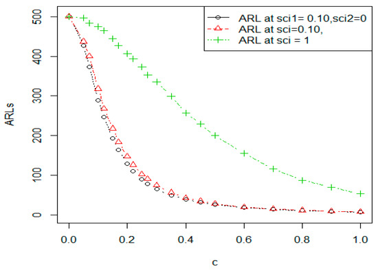
Figure 1.
Graph of comparison of ARLs when .
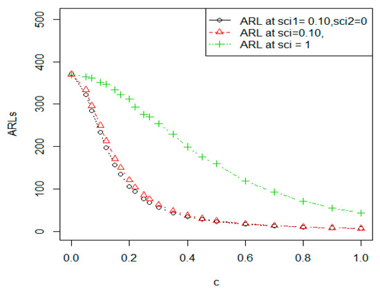
Figure 2.
Graph of comparison of ARLs when .
5. Simulation Study
In order to see the working procedure of the proposed control chart, a simulation study was carried out. For this purpose, we generated 25 observations from a standard normal distribution with a mean of 0 and a standard deviation of 1 for in-control process, and the next 25 observations were generated from the shifted process with mean = 0 + c* standard deviation, where . The estimated values of the proposed EEWMA statistic were computed for the selected levels of the proposed control chart parameters with . Similarly estimated values of the existing EWMA statistic were computed with control chart parameters The data and values of the proposed and existing statistics are listed in Table 8, and plotted values of these statistics are shown in Figure 3 and Figure 4. In Figure 3, we noted that the proposed EEWMA control chart detected a shift at the 47th sample, while in Figure 4, the EWMA control chart could not detect the shift. Hence, this shows that the proposed EEWMA control chart has a greater ability to detect smaller shifts earlier, as compared to the EWMA control chart.

Table 8.
Simulated data.
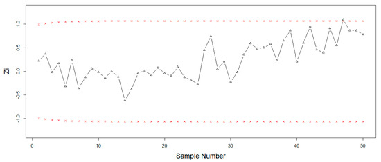
Figure 3.
Graph of simulated data of the proposed EEWMA control chart when .
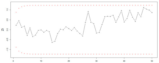
Figure 4.
Graph of simulated data of the EWMA control chart when .
.
.
6. Health-Related Application
Here, we made a comparison of both charts by using application data taken from Santiago and Smith [9]. Data concerned with urinary tract infections (UTIs) were acquired from a hospital. The management of the hospital wanted to know the number of patients being discharged from the hospital who had acquired a urinary tract infection, as a way to rapidly detect the increase in infection rate or, conversely, to observe whether the process resulted in a reduction of infection. As there are different reasons for infection in males and females, this example focused on males. The data entries are listed in Table 9, which follows an exponential distribution with mean time between male UTI patients at 0.21 days or about 5 h. The transformed data into normal distribution was plotted for both EEWMA and EWMA control charts, as shown in Figure 5 and Figure 6. However, the fit in the tails of the distribution is poor, affecting the ability of the control chart to detect process shifts [9]. Both of these graphs shows that the process is in control.

Table 9.
Data of urinary tract infections in patients.
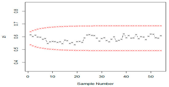
Figure 5.
Graph of real data of the proposed EEWMA control chart when .
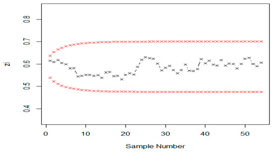
Figure 6.
Graph of real data of the EWMA control chart when .
7. Concluding Remarks
In this paper we presented an EEWMA control chart with the assumption that the quality characteristic of interest follows a normal distribution. ARL tables were constructed for various values of smoothing constants and shifts in the mean. Comparisons were made with EWMA and Shewhart control charts in term of ARL, which showed the ability to detect a shift in the mean more quickly. Application of the EEWMA control chart was also illustrated with the same case study data. The EEWMA control chart can be used in industry for monitoring manufacturing processes. The proposed statistic used in the construction of the control chart can be further extended to the hybrid exponentially weighted moving average statistic Haq [10,11] in future research. The comparison of the proposed chart with an EWMA chart with six or more increasing values in a row can also be studied in future research. The proposed control chart can also be extended by considering the most desirable control chart parameter in future research.
Author Contributions
Conceived and designed the experiments, M.N., M.A. (Muhamma Azam), N.K., and M.A. (Muhammad Aslam); Performed the experiments, M.N., M.A. (Muhamma Azam), N.K., and M.A. (Muhammad Aslam); Contributed reagents/materials/analysis tools, M.N., M.A. (Muhamma Azam), N.K., and M.A. (Muhammad Aslam); Wrote the paper, M.N., M.A. (Muhamma Azam), N.K., and M.A. (Muhammad Aslam).
Funding
This work was supported by the Deanship of Scientific Research (DSR), King Abdulaziz University, Jeddah. The author, M.A. (Muhammad Aslam) acknowledges the DSR technical support with thanks.
Acknowledgments
The authors are deeply thankful to the editor and the reviewers for their valuable suggestions to improve the quality of this manuscript.
Conflicts of Interest
The authors declare no conflict of interest.
References
- Roberts, S. Control chart tests based on geometric moving averages. Technometrics 1959, 1, 239–250. [Google Scholar] [CrossRef]
- Steiner, S.H. EWMA control charts with time-varying control limits and fast initial response. J. Qual. Technol. 1999, 31, 75–86. [Google Scholar] [CrossRef]
- Eyvazian, M.; Naini, S.J.; Vaghefi, A. Monitoring process variability using exponentially weighted moving sample variance control charts. Int. J. Adv. Manuf. Technol. 2008, 39, 261–270. [Google Scholar] [CrossRef]
- Yang, S.-F.; Lin, J.-S.; Cheng, S.W. A new nonparametric EWMA sign control chart. Expert Syst. Appl. 2011, 38, 6239–6243. [Google Scholar] [CrossRef]
- Abbas, N.; Riaz, M.; Does, R.J. Mixed exponentially weighted moving average–cumulative sum charts for process monitoring. Qual. Reliab. Eng. Int. 2013, 29, 345–356. [Google Scholar] [CrossRef]
- Abbas, N.; Riaz, M.; Does, R.J. An EWMA-type control chart for monitoring the process mean using auxiliary information. Commun. Stat. Theory Methods 2014, 43, 3485–3498. [Google Scholar] [CrossRef]
- Aslam, M.; Azam, M.; Jun, C.-H. A new control chart for exponential distributed life using EWMA. Trans. Inst. Meas. Control 2015, 37, 205–210. [Google Scholar] [CrossRef]
- Hariba, P.S.; Tukaram, S.D. Economic design of a nonparametric EWMA control chart for location. Production 2016, 26, 698–706. [Google Scholar] [CrossRef]
- Santiago, E.; Smith, J. Control charts based on the exponential distribution: Adapting runs rules for the t chart. Qual. Eng. 2013, 25, 85–96. [Google Scholar] [CrossRef]
- Haq, A. A new hybrid exponentially weighted moving average control chart for monitoring process mean. Qual. Reliab. Eng. Int. 2013, 29, 1015–1025. [Google Scholar] [CrossRef]
- Haq, A. A new hybrid exponentially weighted moving average control chart for monitoring process mean: Discussion. Qual. Reliab. Eng. Int. 2017, 33, 1629–1631. [Google Scholar] [CrossRef]
© 2018 by the authors. Licensee MDPI, Basel, Switzerland. This article is an open access article distributed under the terms and conditions of the Creative Commons Attribution (CC BY) license (http://creativecommons.org/licenses/by/4.0/).