Model Selection and Quality Estimation of Time Series Models for Artificial Technical Surface Generation

Abstract

Standard compliant parameter calculation in surface topography analysis takes the manufacturing process into account. Thus, the measurement technician can be supported with automated suggestions for preprocessing, filtering and evaluation of the measurement data based on the character of the surface topography. Artificial neuronal networks (ANN) are one approach for the recognition or classification of technical surfaces. However the required set of training data for ANN is often not available, especially when data acquisition is time consuming or expensive—as e.g., measuring surface topography. Thus, generation of artificial (simulated) data becomes of interest. An approach from time series analysis is chosen and examined regarding its suitability for the description of technical surfaces: the ARMAsel model, an approach for time series modelling which is capable of choosing the statistical model with the smallest prediction error and the best number of coefficients for a certain surface. With a reliable model which features the relevant stochastic properties of a surface, a generation of training data for classifiers of artificial neural networks is possible. Based on the determined ARMA-coefficients from the ARMAsel-approach, with only few measured datasets many different artificial surfaces can be generated which can be used for training classifiers of an artificial neural network. In doing so, an improved calculation of the model input data for the generation of artificial surfaces is possible as the training data generation is based on actual measurement data. The trained artificial neural network is tested with actual measurement data of surfaces that were manufactured with varying manufacturing methods and a recognition rate of the according manufacturing principle between 60% and 78% can be determined. This means that based on only few measured datasets, stochastic surface information of various manufacturing principles can be extracted in a way that a distinction of these surfaces is possible by an ANN. The ARMAsel approach is proven to provide the relevant stochastic information for the training of the ANN with artificially generated lapped, reamed, ground, horizontally milled, milled and turned surface profiles.

1. Introduction

In surface topography analysis, parameter calculation (such as Ra/Sa, Rz/Sz, Rk/Sk etc.) according to ISO-standards [1,2,3,4] can be challenging for the user. Assistance software systems such as “OptAssyst” can be useful tools for the selection of measurement parameters that are compliant to the existing standardization [5,6]. Correctly applied evaluation procedures are essential in order to achieve a comparability of the results generated by varying measuring instruments [7].

A surface topography measurement device can be used for a broad variety of measurement tasks. The measurement parameters have to be chosen accordingly to the surface type of the measuring object. An automated classification of measurement objects would lead to a safer choice of those parameters. For an automated classification of surface topography data, a method based on artificial neural networks (ANN) can be an option (among other approaches e.g., based on signal processing [8,9]). Neural networks have the advantage that they do not have to be parameterized manually. Since the amount of data required for successful training is large (thousands of measurements), and measurement of topographies is time consuming (and expensive), the generation of artificial training data (simulated data) represents a valid alternative.

With artificially generated surfaces, much training data can be generated at low costs. For its generation, however, information representing the desired surface needs to be provided. Generally, for the description of rough surfaces different approaches have been utilized in the past: amongst others, functional surface characterization and feature-based parameters are a current trend to extract information from a surface [10]. Relevant information for the generation of surfaces has been provided by moving average (MA) models with a defined power spectrum (PSD) [11], auto-regressive (AR) models [12], models based on the autocorrelation function and FFT [7] and probability density functions for simulating a desired height distribution (see [13] for a review). A common approach is the (manual) specification of a defined auto-correlation function (ACF) or power spectral density (PSD), as for example suggested by Wu [14]. The reason is that both the PSD and ACF contain integral information about the surface characteristics as they are related by the Fourier Transform [15]. Jacobs et al. provided a detailed examination of the application of the PSD in surface topography measurement [16]. Krolczyk et al. used the PSD function for the comparison of different surfaces [17].

With the approach described by Wu also a simulation of surfaces that have a non-Gaussian height distribution is possible, a type of surface which has as well been addressed in various other studies [18,19,20]. Generally, the manufacturing principle does not only influence the height distribution but also other surface texture features such as the directionality (see e.g., [21]). Other approaches for the modeling of surface roughness are the extraction of information of a time series by if-then-rules [22], the use of stochastic surface features [23] and models for non-linear dynamical systems [24].

A successfully trained classifier for surface type recognition for a two-class-problem based on artificially generated ground and honed surfaces, which can be applied to measurement data with an appropriate classification rate, has been shown in previous work. For the calculation of the profiles which served as training data, a model based on a known autocorrelation function (ACF) was chosen as input data [7]. The disadvantage of the model presented in [7] is that it is not based on real measurement data and that it requires manual parametrization.

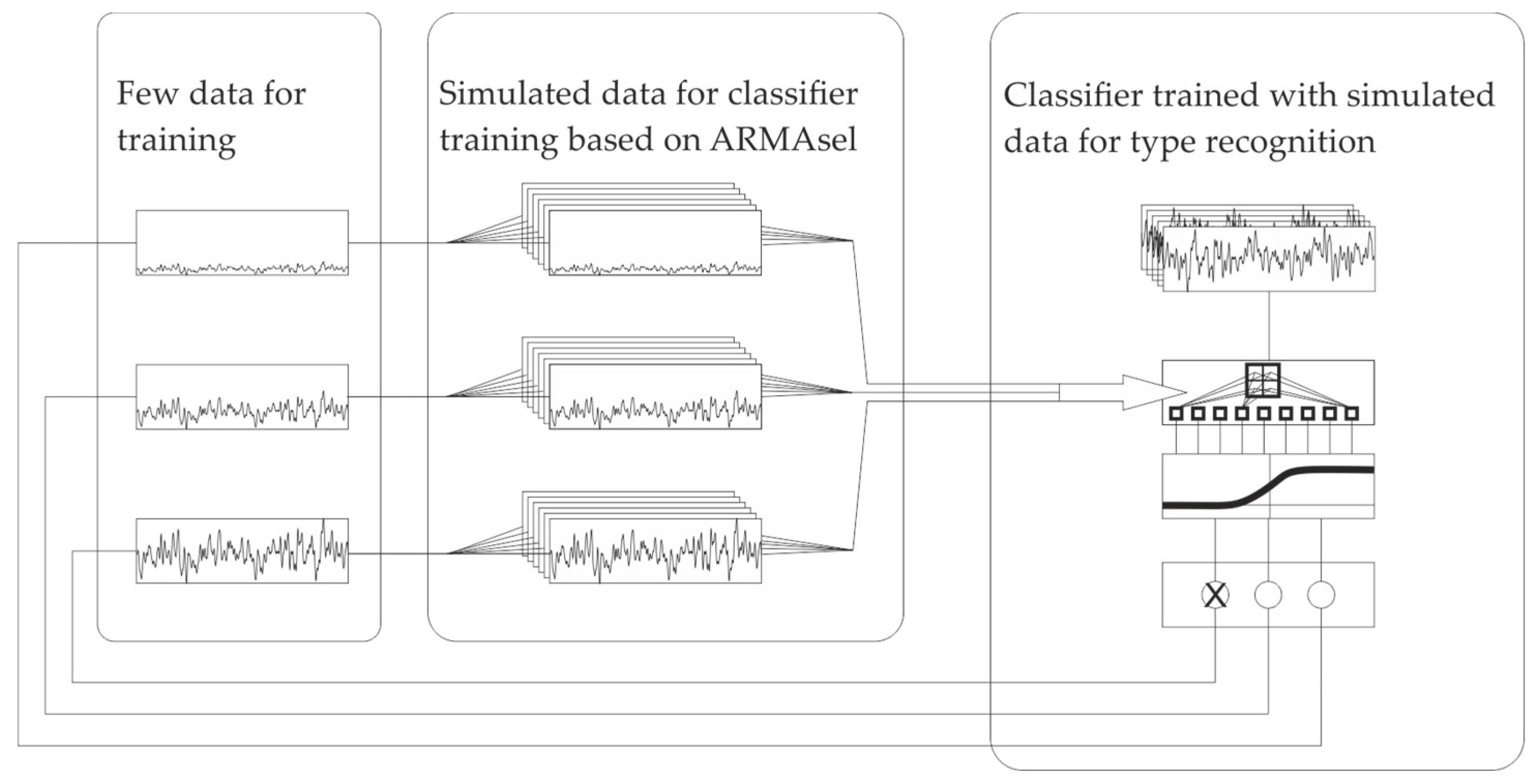
Hence, we propose a method that simulates the training data for the classifiers based on the measurement data of component surfaces. The calculated time series model coefficients from few sample data can serve as input for the generation of artificial surfaces that are then used for the training of classifiers for an ANN (Figure 1). Auto-regressive (AR), moving average (MA) and auto-regressive moving average (ARMA) models have been previously applied for the characterization of rough surfaces and the statistical description of roughness (see e.g., [11,12,25]). We propose an approach based on the ARMAsel model presented by Broersen [26] which can find the best possible time series model for an accurate description of a measured surface.

With the time series model, the frequency properties of the surface can be calculated. Thus, it is possible to provide a statistical description of real engineering surfaces which serves as input data for a sound calculation of artificial surfaces. An improved description of technical roughness compared to intuitively selected models and numbers of parameters can be achieved. The quality of the models is evaluated and recommendations for the description of roughness are presented.

Amongst others, Seewig proposed the combined auto-regressive moving average (ARMA) model, which describes a roughness profile $r$ by the $N_{AR}$ auto-regressive coefficients $A{R}_j$, the $N_{MA}$ moving average coefficients $M{A}_j$ and a Gaussian-distributed noise vector $n$ [25]:

$$r_k+{\displaystyle \sum _{j=1}^{N_{AR}}{r}_{k-j}}\cdot A{R}_j=n_k+{\displaystyle \sum _{j=1}^{N_{MA}}{n}_{k-j}}\cdot M{A}_j$$

(1)

By setting $A{R}_j=0$, the model can be transformed into a moving-average model and by $M{A}_j=0$ into an auto-regressive model. Thus, the ARMA-model represents a superposition of both approaches. As a rule of thumb, 5–10 coefficients are sufficient for the modeling of rough surfaces [25,27], but there exist approaches for choosing the optimal number of coefficients. One of those is investigated in the following paragraphs.

Thus, the description of known surfaces with time series models is analyzed in depth. In doing so, different AR-, MA- and ARMA-models are used to determine the most accurate description of different types of rough surfaces which were manufactured with a broad range of manufacturing principles. The optimal model and number of coefficients is chosen. The objectives are achieved by utilizing the ARMAsel-model [26] which is described in the following Section 2 and applied to surfaces with varying manufacturing methods in Section 3. The resulting coefficients provide an accurate description of the statistical properties of a certain manufacturing principle whose quality is examined in Section 4. This information can be used for the generation of multiple artificial surfaces with the same statistical properties which serve as training data for an ANN described in Section 5.

2. The ARMAsel-Approach

The ARMAsel-approach was suggested by Broersen and is capable of automatically selecting a time series model based on statistical criterions [26]. Different AR-, MA- and ARMA-models with a varying number of coefficients are calculated and the prediction error of all models is determined in order to select the model that features the smallest prediction error [26]. The prediction error $PE(N_{AR})$ for an AR-model of the order $N_{AR}$ can be determined based on the residual variance $res(N_{AR})$ and $K$ data points [26,28]:

$$PE(N_{AR})=\left\{res(N_{AR})\right\}{\displaystyle \prod _{j=1}^{N_{AR}}\frac{1+1/(K+1-j)}{1-1/(K+1-j)}}$$

(2)

The MA-model of the order $N_{MA}$ and the ARMA-model of the orders $(N_{AR},N_{AR}-1)$ can be evaluated based on the number of parameters $N$ [26,29]:

$$PE(N)=\left\{res(N)\right\}\frac{1+N/K}{1-N/K}$$

(3)

The selected model (referred as ARMAsel) of all calculated AR-, MA- and ARMA-processes is the one with the smallest prediction error and thus its determination relies solely on statistical properties [26]. The definition of the ARMAsel-approach is provided for arbitrary time series. However, an application for the description of roughness has not yet been examined extensively. In the following section, the algorithms will be applied for the description of varying rough surfaces with different roughness parameters. In doing so, the best possible model for the most accurate statistical description of a present surface is estimated. This determined model serves as initial point for the calculation of the AR-, MA- or ARMA-coefficients and a subsequent generation of artificial surfaces with desired stochastic properties.

3. Applying the ARMAsel Algorithm for the Description of Rough Surfaces

As stated, an examination of the ARMAsel-approach is useful as the best model with the smallest prediction error and the required number of parameters can be chosen automatically based on objective criteria. Thus, an improved description of technical roughness compared to traditional models and their parameters, which are often being selected intuitively, can be achieved.

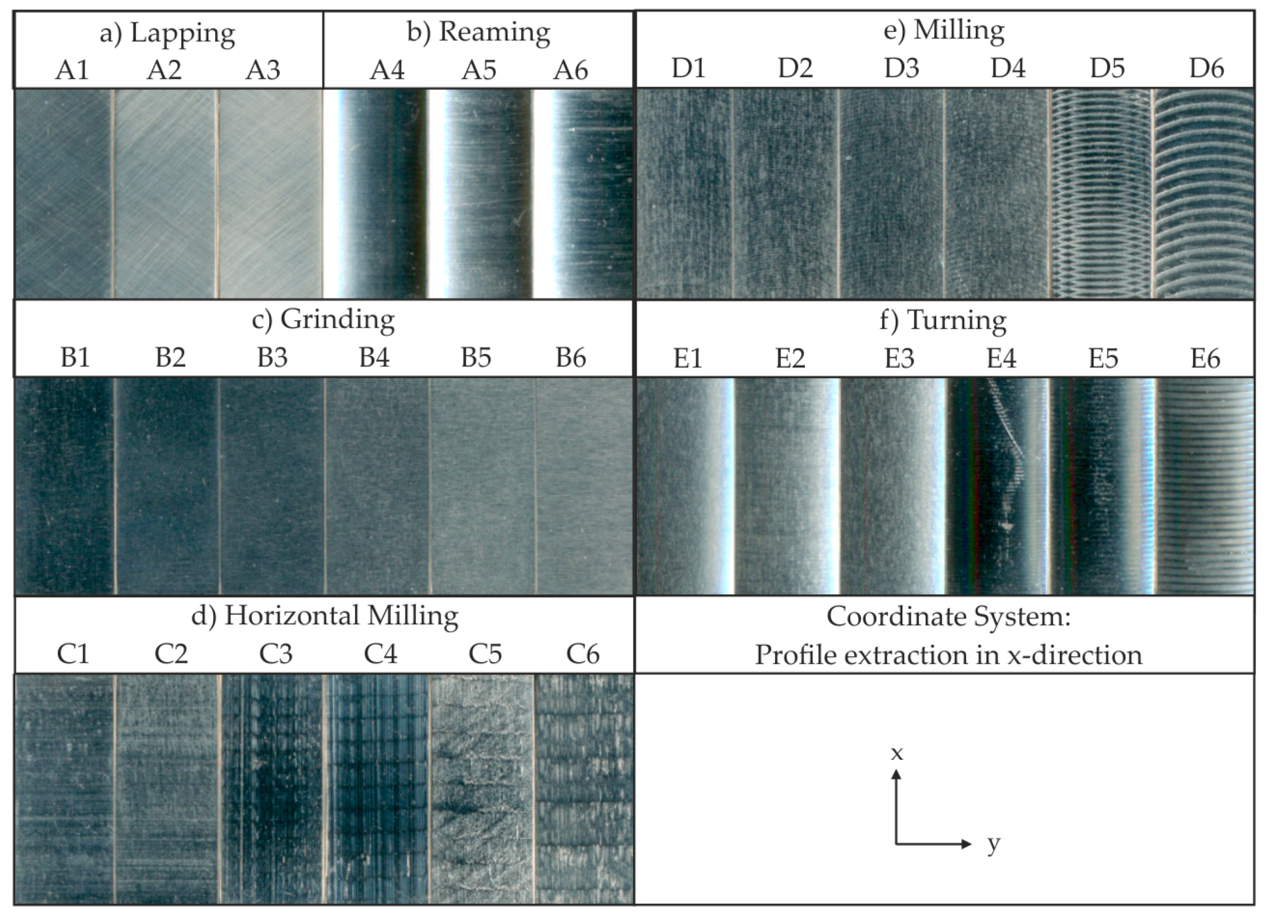
In order to test the model with a broad range of different surfaces, the roughness specimens set Rubert 130 was chosen, which features typical engineering surfaces and represents the most relevant manufacturing principles: Turning, Milling, Horizontal Milling, Grinding, Lapping and Reaming [30]. The different manufacturing principles are given in varying degrees of roughness, leading to a total number of 30 different rough surfaces (see [30]) from six classes. All 30 samples and their nomenclature are shown in Figure 2 and were measured with a stylus instrument (Hommel Nanoscan) with a 5 µm stylus tip. The measured dataset was filtered and examined with the ARMAsel algorithm by Broersen [26,28,31,32]. The required ARMAsel algorithms and their implementation are available within the ARMASA-toolbox for MatLab [33].

For the examination, 50 different evaluation positions on each of the 30 samples with a lateral distance of 200 µm to each other and an evaluation length of 4 mm were considered and used as input data of the ARMAsel algorithm. For the evaluation, the selection of the best model, the prediction errors of the best AR-, MA- and ARMA-model and the chosen number of AR- and MA-coefficients were considered. Thus, the result for each sample A1–E6 are the 50 chosen models for all 4 mm evaluation profiles, the prediction error for the varying time series models and the according AR-, MA- or ARMA-coefficients for each evaluation. Due to the filtering process before the evaluation with the ARMAsel-algorithm, waviness components are removed from the measured dataset and are not modeled with the stochastic models. The default filter wavelength is chosen to ${\lambda }_c=0.8\mathrm{mm}$. For some rough structures that have characteristic long-wave machining marks based on the feed-rate, the filter wavelength is adjusted so that the features which are characteristic for the considered manufacturing process are not removed from the dataset (this affects the profiles C3–C6 and D6).

3.1. Lapped Surfaces (A1–A3)

The three different lapped surfaces shown in Figure 2 were evaluated with the ARMAsel algorithm. The surface Lapping A1 is the finest surface, whereas the surface Lapping A3 is the one with the biggest roughness (Figure 3a,b). The results for the selected models with the smallest prediction error (Figure 3c), the absolute values of the prediction errors (Figure 3d) for the selected models and for the best AR-, MA- and ARMA-models are given in Figure 3 as well as the selected number of parameters for each model category (Figure 3e). There, the model selection of the profiles A1–A3 is indicated as well as the prediction error of the varying time series models. All results are presented as mean value and standard deviation of all evaluations of the 50 evaluation areas which feature a length of 4 mm each and thus cover the whole measuring length of approximately 14 mm. The results show that AR-, MA- and ARMA-models are suitable for a description of lapped surface roughness and feature similar values of the prediction error. For the description of the fine roughness, the AR-model is the model which is chosen the most often. Figure 3 illustrates the whole measuring length of the profiles Lapping A1 and Lapping A3 and displays the according results of the different time series models for all 50 evaluations of each sample.

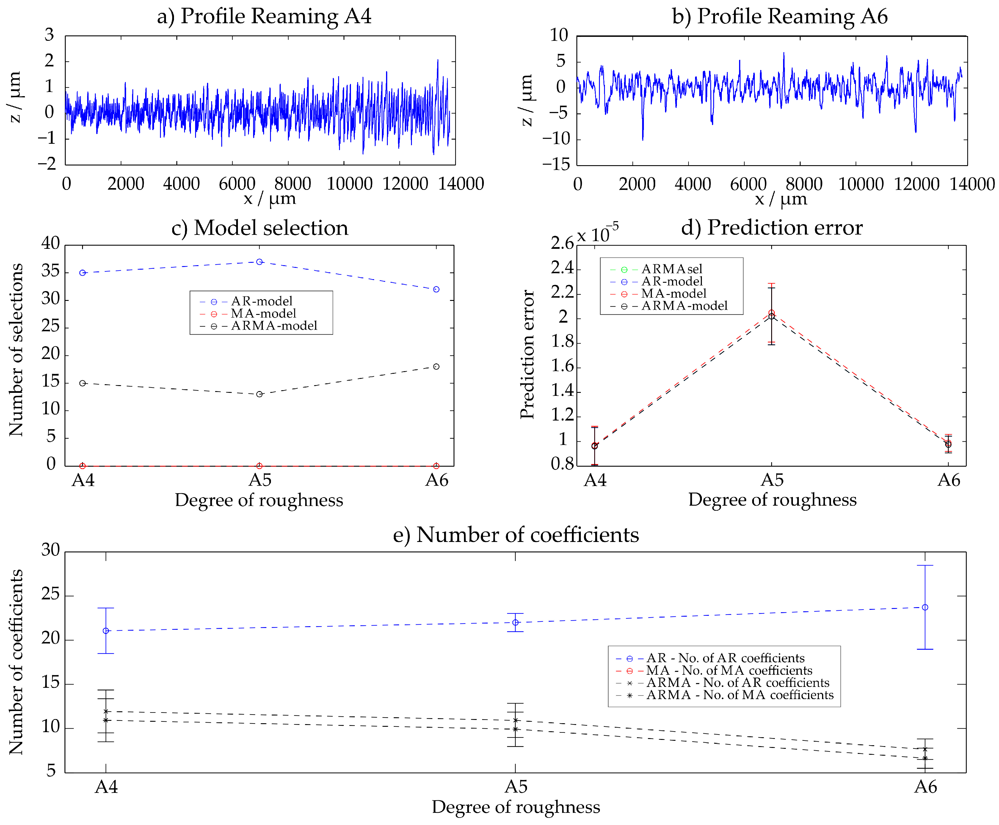
3.2. Reamed Surfaces (A4–A6)

Three different reamed surfaces A4–A6 of the Rubert roughness specimens were examined. The detailed results are given in Figure 4 for all 50 evaluations of each sample. Generally, all three different models AR, MA and ARMA lead to comparable prediction errors for all three surfaces. The surfaces have a stochastic character and can thus be described easily with the different statistical models. The following tendency can be observed: the rougher the profile is, the fewer coefficients of the ARMA-model are required for the description. As models, both AR- and ARMA-models are selected as models with the smallest prediction error.

3.3. Ground Surfaces (B1–B6)

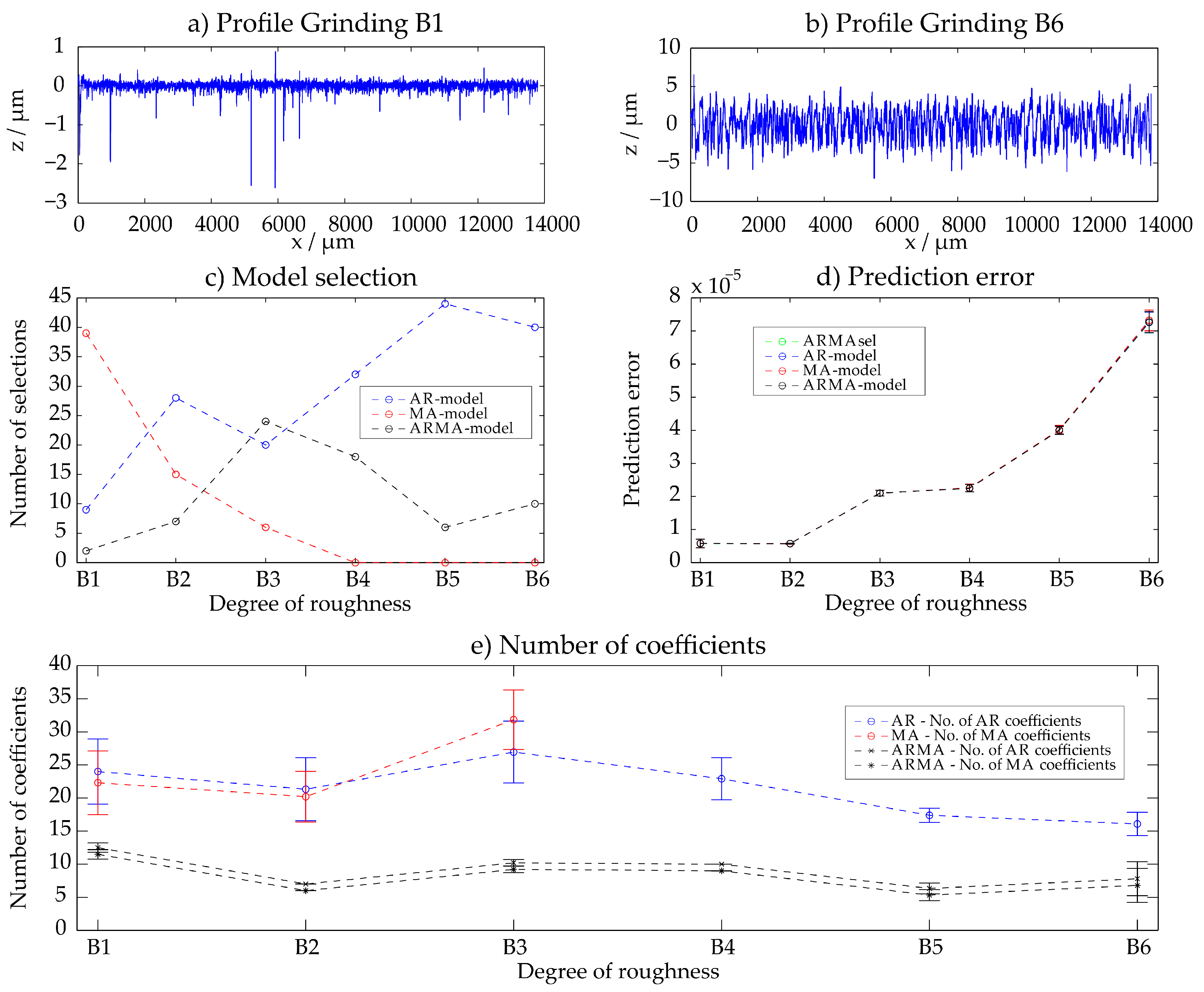
The Rubert set of roughness specimens contains six different ground surfaces B1–B6. The observation can be made that for finer surfaces the MA-model has the smallest prediction error, whereas for rough surfaces an AR-model is more suitable. This effect might as well be caused by the discontinuities of the profile B1 (see Figure 5a). As an example, for the sample B6 the AR-model has the smallest prediction error in about 40 of the 50 evaluated areas. All results are illustrated in Figure 5. For the rougher surfaces, the prediction error increases as shown in Figure 5d. The number of coefficients generally decreases with increasing roughness (Figure 5e). Also here, due to the stochastic character of the surface, a small number of parameters is sufficient for an adequate stochastic description.

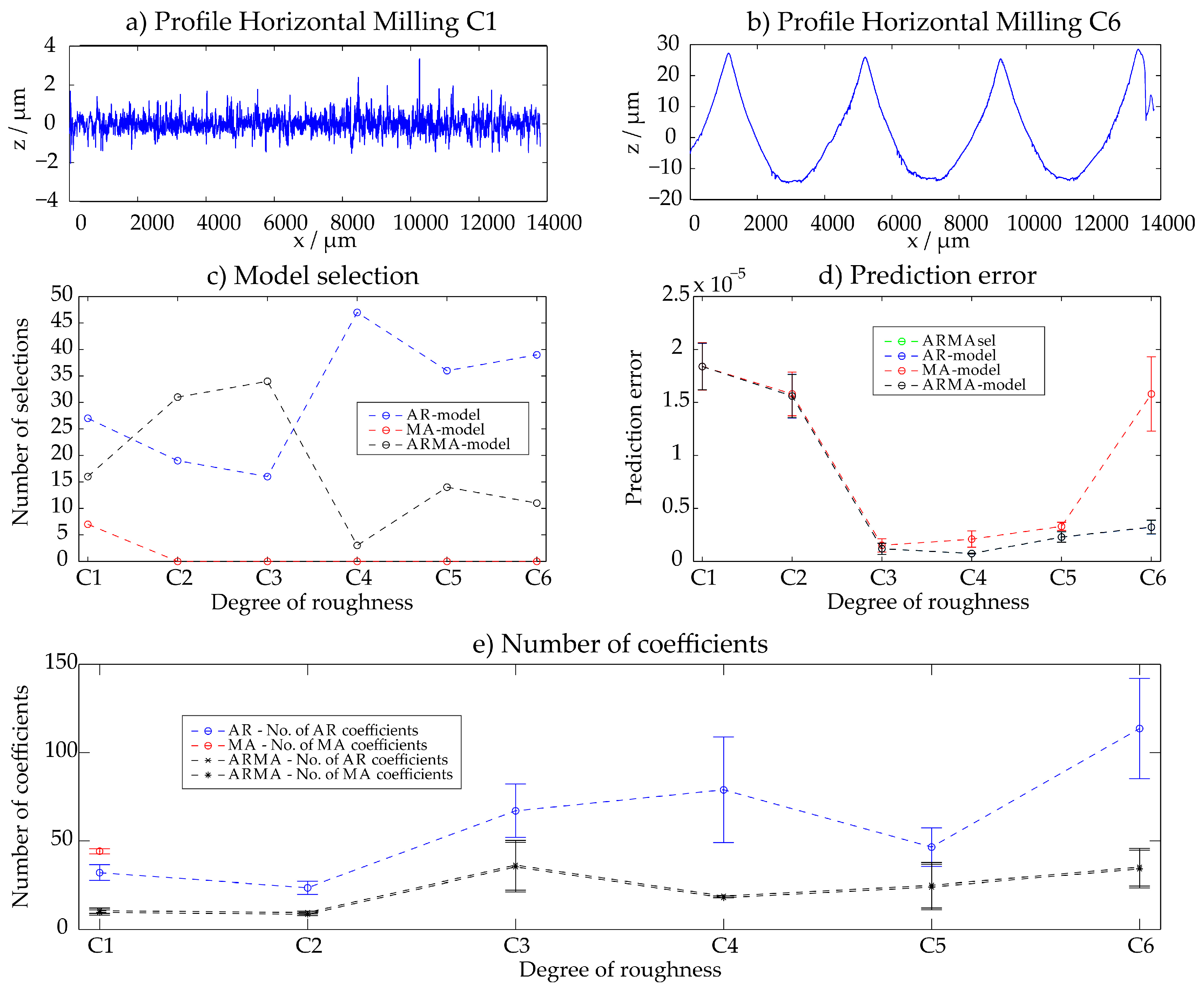
3.4. Horizontally Milled Surfaces (C1–C6)

The manufacturing method of horizontal milling was as well examined with six different samples C1–C6 and 50 evaluations each. Contrary to the manufacturing principles which lead to a stochastic surface, the number of required coefficients increases with a rougher surface. The reason is that the deterministic shape of the grooves becomes more and more visible with increasing roughness. The results are given in Appendix A. For the finer surfaces, all three approaches lead to similar results. For rougher surfaces, the AR- and ARMA-model feature the smallest prediction error. As the rough surfaces manufactured with horizontal milling exhibit long-wave components, the filter wavelengths of the samples Horizontal Milling C3–C6 were adapted to larger values.

3.5. Milled Surfaces (D1–D6)

Fine and rough milled surfaces D1–D6 were examined. All results are summarized in Appendix A. Similar results as with the horizontal milling process can be observed: with increasing roughness the deterministic structure is more significant and also more parameters are necessary for the description. AR-, MA- and ARMA-processes have all similar prediction errors. The filter wavelength in the pre-processing of the sample Milling D6 was increased, analogously as for samples C3–C6.

3.6. Turned Surfaces (F1–F6)

For the six different turned surfaces, the AR-model and ARMA-model are selected. The prediction error of the AR- and ARMA-models is similar and also the MA-model does not differ significantly for most surfaces. The results are summarized in Appendix A. For fine surfaces, many parameters are required for an accurate description due to the high complexity of the surface. For rougher surfaces, the deterministic pattern of the surface leads in contrast to other manufacturing principles to a reduced number of parameters. This indicates that the complexity of a surface has a higher impact on the number of parameter than its character.

Generally, it can be shown that for all examined surfaces, an adequate stochastic description of the surface properties is possible based on the ARMAsel approach. In order to evaluate the quality of the selected models, further considerations have to be taken into account.

4. Model Evaluation

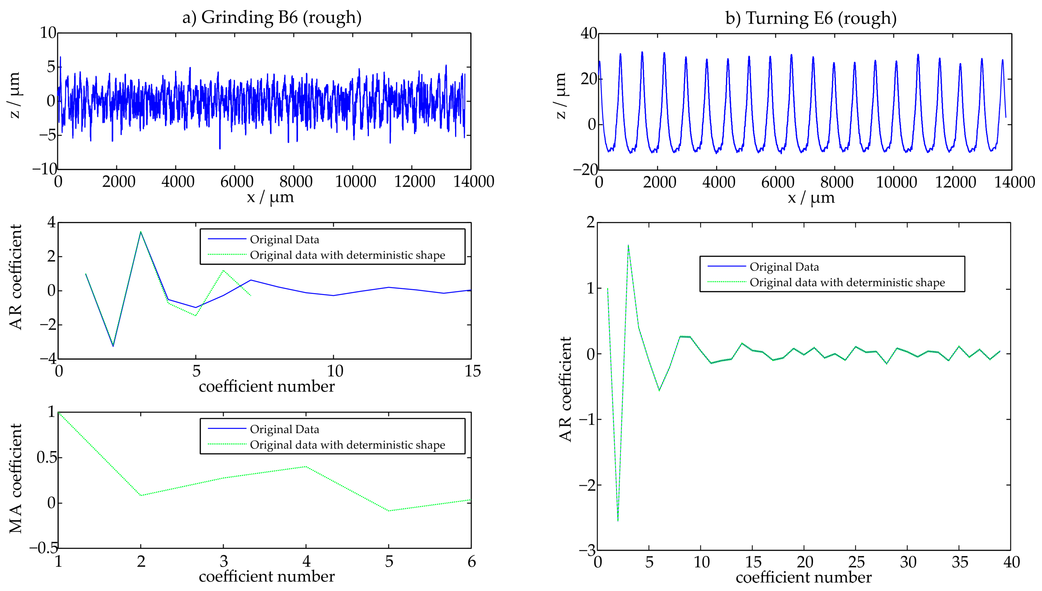
In order to examine the quality of the calculated models, different criteria are suggested. As a first quality indication, the stability of the calculated coefficients is determined. In doing so, the values of the AR- and MA-coefficients are analyzed. These coefficients are determined for a selected profile. Then, this profile is superposed with a long-wave sinusoidal structure that features a wavelength of 8 mm and the values of the coefficients are determined once more. When the coefficients are compared, the robustness of the model can be evaluated. If the two sets of coefficients are in good agreement, the model is robust. When the coefficients differ significantly, the model is not robust as small form distortions should only change the coefficients with a low index. Figure 6 illustrates the comparison for a stochastic ground surface (B6) and a more deterministic turned surface (E6). The coefficients are determined before and after adding the sinusoidal wave. This is done to characterize the effect of the deterministic structure on the model. An exemplified evaluation of one 4 mm extract of the measured profile is illustrated in Figure 6 for the profiles B6 and E6.

When for example the stochastic profile Grinding B6 is examined, the coefficients do change as the ARMA-model is chosen instead of the AR-model and only few coefficients are necessary for the description of the surface. For the deterministic surface however the coefficients do not change as significantly, as the same model is chosen and the profile already features deterministic characteristics before the sinusoidal wave is added. Also, the number of coefficients is significantly higher than for the ground profile.

As a second criterion, the quality estimation of the proposed models is performed by the evaluation of the power-spectral-density (PSD). The PSD can be obtained directly from the roughness profile $\overrightarrow{z}=z_n,n=1,\dots ,N$ based on its discrete Fourier transform (DFT) with the coefficients $X_k$:

$$X_k={\displaystyle \sum _{n=0}^{N-1}{z}_n^{}\cdot e^{\frac{-i\cdot 2\pi \cdot k\cdot n}{N}}},n=1,\dots ,N,k=0,\mathrm{\dots },N-1.$$

(4)

The PSD of the profile $PSD{P}_k$ can be calculated from the DFT as follows [34]:

$$PSD{P}_k=\frac{1}{2\pi \cdot N}{\left|X_k\right|}^2,k=1,\dots ,\frac{N}{2}+1.$$

(5)

In the given definition a factor of 2 needs to be applied in order to ensure the total power conservation as only one half of the frequencies need to be examined for real-valued signals [34]:

$$PSD{P}_k=2\cdot PSD{P}_k,k=2,\dots ,\frac{N}{2}+1.$$

(6)

With the normalized frequencies:

$$\overrightarrow{\omega }=\frac{{\omega }_k}{\pi },{\omega }_k=(k-1)\cdot \frac{2\pi }{N},k=1,\dots ,\frac{N}{2}+1.$$

(7)

and the logarithmic definition of the power:

$$P\overrightarrow{S}D1=PSD{1}_k,PSD{1}_k=10\cdot {\log }_{10}\left(PSD{P}_k\right)k=1,\dots ,\frac{N}{2}+1.$$

(8)

the normalized PSD $PS{D}_P$ which is based on the profile is defined as:

$$PS{D}_P=\left(\overrightarrow{\omega },P\overrightarrow{S}D1\right).$$

(9)

The PSD can as well be obtained from the ARMA-coefficients (see e.g., [35]). When the two PSDs are compared with each other, a quality criterion for the ARMA-Model and its coefficients can be obtained. The PSD based on the ARMA-coefficients can be calculated with the variance ${\sigma }_e^2$ of the stochastic input signal and the coefficients $A{R}_j$ and $M{A}_j$ [32,35]:

$$P\overrightarrow{S}D2=\frac{{\sigma }_e^2}{2\pi }\cdot \frac{{\left|1+{\displaystyle \sum _{j=1}^{N_{MA}}M{A}_j}\cdot e^{-i\omega j}\right|}^2}{{\left|1+{\displaystyle \sum _{j=1}^{N_{ARA}}A{R}_j}\cdot e^{-i\omega j}\right|}^2}.$$

(10)

When this second PSD is as well normalized:

$$P\overrightarrow{S}D2=PSD{2}_k,PSD{2}_k=10\cdot {\log }_{10}\left(PSD{2}_k\right)k=1,\dots ,\frac{N}{2}+1,$$

(11)

a direct comparison to the PSD obtained from the profile is possible in order to perform a model evaluation.

For the determination of both PSDs the same frequencies are used in order to ensure the best possible comparability. Then for the comparison, the average squared deviation between the two PSDs is calculated for all 50 calculated PSDs of each evaluated profile extract and is defined as an evaluation criterion:

$$dev=\frac{{\displaystyle \sum _{j=1}^{N/2+1}{\left(PSD{1}_j-PSD{2}_j\right)}^2}}{N/2+1}.$$

(12)

The results of the deviations for the examined profiles are given in

Table 1. Averaged squared deviations between PSD functions in (db/rad)².

	1 (Fine)	2	3	4	5	6 (Rough)
Lapping A1–A3	793.43 ± 145.66	442.52 ± 126.41	241.82 ± 92.57	-	-	-
Reaming A4–A6	-	-	-	125.79 ± 54.51	252.67 ± 186.56	450.03 ± 241.73
Grinding B1–B6	599.20 ± 168.52	449.88 ± 130.49	190.59 ± 81.91	107.40 ± 40.61	120.47 ± 75.34	254.55 ± 167.72
Horizontal Milling C1–C6	128.49 ± 53.65	119.42 ± 65.36	633.30 ± 308.22	845.03 ± 386.99	2365.10 ± 799.30	1375.94 ± 539.69
Milling D1–D6	118.06 ± 38.05	176.06 ± 98.03	317.77 ± 212.99	756.30 ± 398.38	1455.34 ± 479.92	2335.25 ± 688.24
Turning E1–E6	126.57 ± 44.75	132.47 ± 73.99	192.15 ± 127.93	1287.04 ± 418.82	1864.56 ± 522.53	2594.69 ± 802.70

. There, the value of $dev$ is presented as a mean value and standard deviation of all 50 evaluation areas of each sample. It can be observed that there is no direct correlation between the degree of roughness and the deviation. However, it can be stated that the more stochastic surfaces do have a better agreement between the two PSD functions. Generally the ground surfaces show the best compliance, whereas the turned surfaces which have a very distinct deterministic structure feature the highest deviations of the PSDs.

This observation can be verified when the different PSDs are directly compared as shown exemplary in Figure 7. When the stochastic ground surface is examined, there is a high compliance between the two sets of PSDs, whereas when the deterministic turned surface is evaluated, the difference between the two sets of PSDs is significant. Figure 7 illustrates and compares all 50 evaluated PSD functions for the two surfaces.

Based on the PSD of a surface, for example also its ACF can be calculated trough an inverse Fourier transform. The ACF can then also be used for generation of artificial surface data which has the same statistical properties such as the original measured dataset [7]. As shown the approach of the time series model determination works especially accurate for stochastic surfaces. Deterministic surfaces lead to higher deviations between the PSD functions of the determined coefficients and the profile.

In the following, the profile generation based on the determined AR-, MA- and ARMA-coefficients is examined. As the ARMAsel algorithm allows the determination of an optimum time series model for a given surface and thus includes all relevant stochastic surface properties, it can be applied for the training of classifiers for an artificial neural network (ANN) as a big number of test profiles can be generated based on the given stochastic properties. With the quality of the ANN, it can also be examined in which way a single profile is characteristic for an entire manufacturing process.

5. Training of Classifiers with Simulated Data

The techniques described in the previous sections can be used to generate a variety of profiles with the predefined characteristics of technical surfaces using only one measurement as input. The idea behind this approach is to train classification systems for the recognition of technical surface types, for example in order to support measurement technicians, even when only a small amount of training data is available [7]. Artificial neural networks (ANN) are an approach to the implementation of classifiers based only on measurement data sets and are therefore an alternative to signal processing approaches. Specifically convolutional neural networks (CNN) are successfully used to classify images, for example for the recognition of handwriting [36] or for recognizing objects in images [37]. Since profiles extracted from technical surfaces can be interpreted as 1D-grayscale images, the transfer of these techniques is evident.

5.1. Training Data Generation

The techniques described above (Section 1, Section 2 and Section 3) are applied for the generation of artificial data sets with the characteristics of the examined lapped, reamed, ground, horizontally milled, milled and turned surfaces of Section 3. This means, the Rubert standard 130 is selected as data population source: the standard features six different manufacturing processes, each in three to six degrees of roughness (two times three degrees, four times six degrees, in total 30 different samples from six processes as shown in Figure 2). For each of the 30 samples the 50 different evaluation areas that were extracted from different locations of a tactile measured dataset used with the ARMAsel algorithm. In doing so, the stochastic properties of the surface as described in Section 3. For the generation of artificial test profiles, the AR-, MA- or ARMA-coefficients of the first profile were chosen. The coefficients of the selected model (ARMAsel) with the smallest prediction error did serve as input parameters for the training data generation. A gaussian-distributed random number is generated with the length of $n$ profile points and is normalized with the number of profile points:

$${\overrightarrow{z}}_{rnd}=z_{rnd}(i),i=1,2,\dots ,n,z_{rnd}(i)=\frac{z_{\sigma }}{n}.$$

(13)

$z_{\sigma }$ is a normal-distributed random value. With the $N_{AR}$ AR-coefficients $A{R}_j,j=1,2,\dots ,N_{AR}$ and the $N_{MA}$ MA-coefficients $M{A}_j,j=1,2,\dots ,N_{MA}$ of the ARMAsel-model, the transfer function $G(z)$ in the $z$-domain of the relevant stochastic surface characteristics is calculated as:

$$G(z)=\frac{{\displaystyle \sum _{j=1}^{N_{MA}}M{A}_j\cdot z^{-j+1}}}{1+{\displaystyle \sum _{j=2}^{N_{AR}}A{R}_j\cdot z^{-j+1}}}.$$

(14)

In order to simulate the training profiles according to the transfer function, the convolution theorem is used and the randomly distributed initial data is filtered with the function defined in Equation (14). The resulting profile ${\overrightarrow{z}}_{test}=z_{test}(i),i=1,2,\dots ,n$ is normalized to the interval [−1, 1]. Afterwards, the test profiles are converted into a [0, 255] grayscale image.

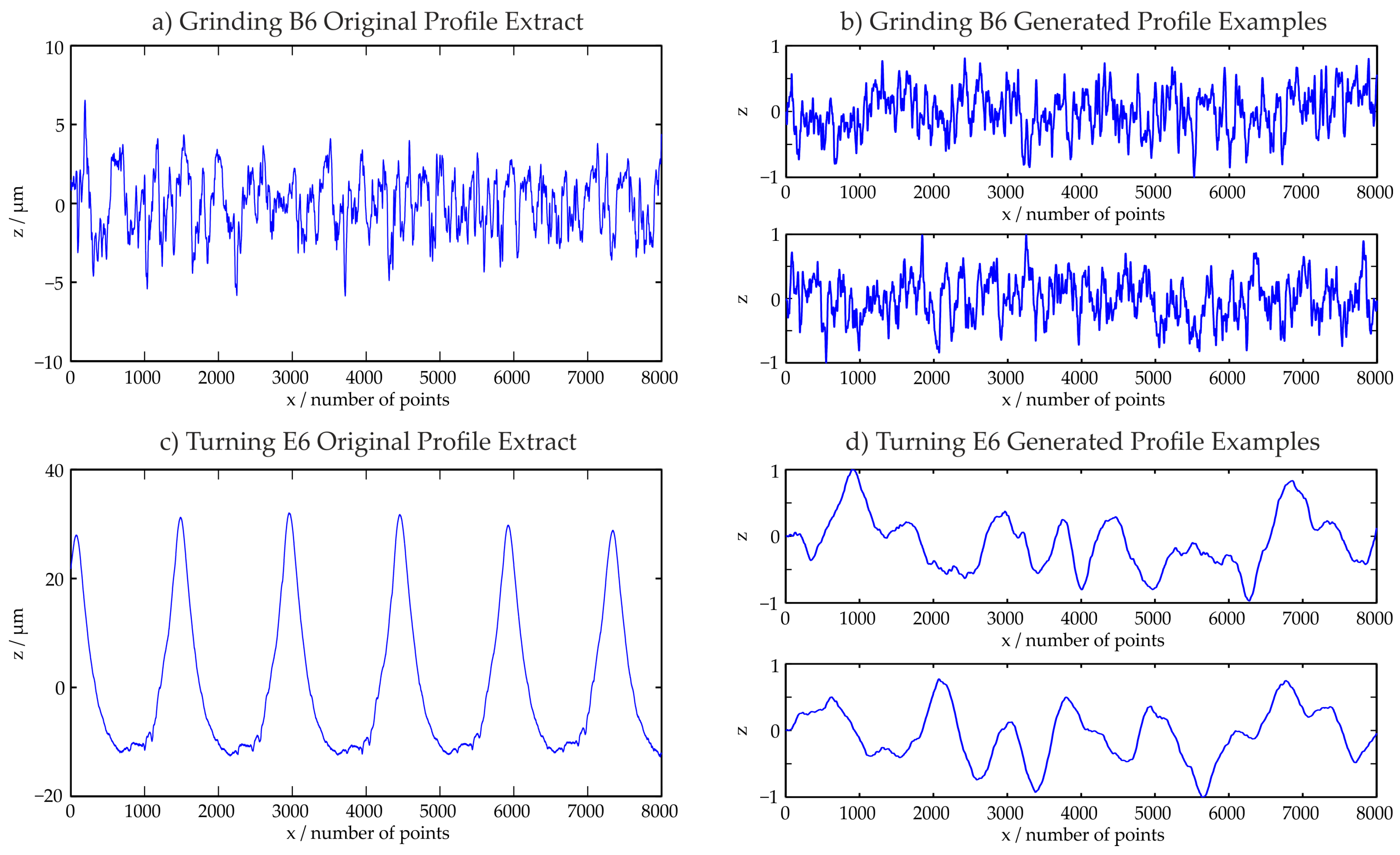
Figure 8 shows examples for generated training profiles. Figure 8a displays the first evaluation area of the profile type Grinding B6 which was utilized for the training data generation. In Figure 8b, two examples for resulting, normalized generated profiles are shown. When a very deterministic profile as the profile Turning E6 in Figure 8c is used, the resulting profiles shown in Figure 8d differ more from the original profile. This is in compliance with the observations made during the model quality estimation in Section 4. The time series models are most accurate for the description of stochastic surface structures.

In total, 7000 profiles are generated for each degree of each manufacturing process (30 × 7000 = 210,000 datasets), which are split into 5000 profiles per class for training (overall 150,000 profiles) and 2000 profiles for testing (overall 60,000 profiles). The 30 × 50 = 1500 actual measured extracts of the Rubert samples are kept for test after training the CNN. In this way it can be examined whether the stochastic data of a single measurement which can be representative for an entire manufacturing process or not. This can be measured with the recognition rate of the actual measured profiles. The CNN architecture is described in the following.

5.2. CNN Architecture, Traning, and Weights Discussion

For the classification task, a multi-layer Convolutional Neuronal Network (CNN) is used, similar to the ones applied to the recognition of features in images. The convolution operators (or their learned weights) serve to detect features in the data, regardless of their spatial position. This applies well for technical surfaces, which are mostly stochastic and/or periodic, thus making the spatial position of a feature irrelevant. The idea behind a multi-layer approach is that on the early layers simple features such as edges are learned. On the deeper layers these simple elements are combined to more complex structures. Since no highly complex structures are expected in the data and training effort increases with additional levels, only three layers are selected. The convolutional operators are followed by a layer for classification.

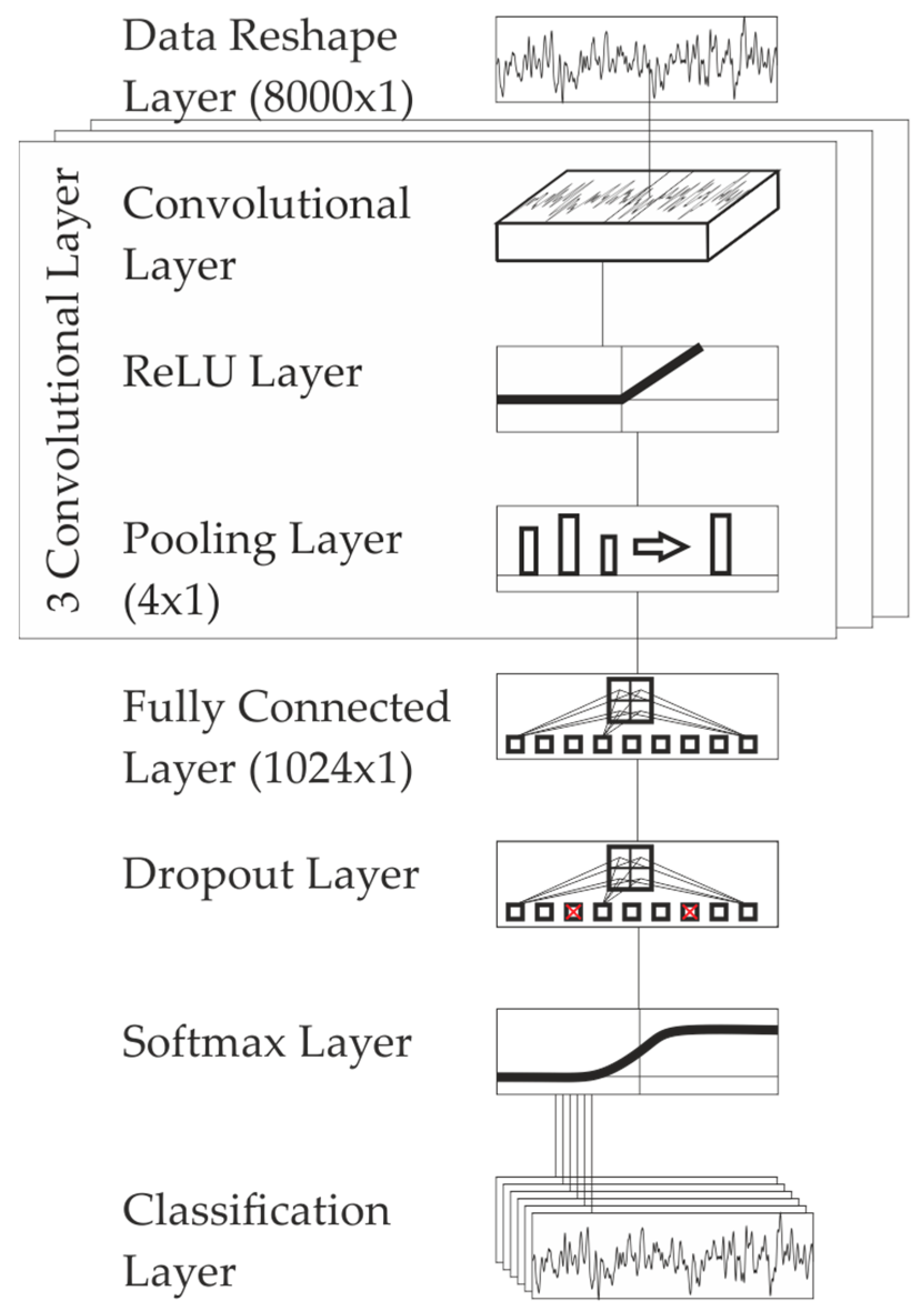
The architecture of the selected convolutional neural networks is as follows: as pre-processing, the generated profiles (see Section 5.1) are normalized and converted to 8-Bit-grayscale image [0, 255] of the size 8000 × 1. This is done in order to eliminate the influence of the absolute signal amplitude in the data, hence putting a focus on the relative parts of the signal.

The preprocessed profile data is fed to the first convolutional layer with 16 filters of size 10 × 1, followed by a rectified linear unit (ReLU) Layer and a max-pooling operator with size 4 and a stride 4, which reduces the first-layer data vector to a vector of size 2000 × 1. The 2nd and 3rd layer are structured in a similar way: the 2nd and 3rd convolution is each being followed by a ReLU layer and max-pooling operator, thus the final feature vector size is 125 × 1 (the original data is reduced by 4^{(nlayers−1)} = 16). The combination of convolution, ReLU layer and pooling is expected to preserve important information while reducing the overall data volume, resulting in a reduction of computation time [38]. The filter sizes are 10 × 1, the number of filters is 32 in the 2nd and 64 in the 3rd layer. The idea behind the constant filter sizes, in combination with the pooling layer is to see local features on the first layer of the CNN and more global features on the third layer of the CNN. The 16 × 125 feature vector is mapped to a 1024 × 1 fully connected layer, which is followed by a dropout layer with 20% dropout probability. The dropout layer is introduced with the idea to prevent overfitting in the model [39]. A visualization of the architecture is given in Figure 9. After the dropout-layer, a SoftMax layer is introduced for classification, which maps the output of the dropout layer to the range [0, 1].

The architecture is implemented in and trained with Python 3.5.4 and Tensorflow [40] version 1.3.0. The training process featured 2000 and 20,000 steps, with 200 randomly chosen training samples per step and a learning rate of 0.001.

Variations in the CNN architecture and training parameters were taken into account, such as varying layers (2 two and three layers), varying filter sizes (range: 5 × 1–5ilities0 × 1), varying filter numbers (2–64 filters), varying sizes for the fully connected layer (128–2048), varying dropout probab (10–20%), varying number of training samples per iteration (50–500), varying training steps (500–20,000), but resulted in similar or slightly worse classification performance, and are thus no subject to further discussions.

5.3. Classification Performance

Two different sets of training data are considered: First, all the available training data of all samples (30 × 5000 = 150,000 profiles) is used for training the CNN. In doing so it is checked if the (preprocessed and scaled) simulated data is of sufficient quality for training the classifiers and thus representing the real data. For this case, it is expected that the CNN will receive a high classification rate, close to our previous results (~80%) [7].

In the 2nd experiment, the set of training data is reduced to simulated data from the middle degree of roughness (4th degree for 6 degrees, 2nd grade for 3 degrees) which leads to 6 classes, each with 5000 training samples and 30,000 overall profiles for training. This is done to investigate if the CNN can learn a generalized surface model for a manufacturing process from limited training data. The classifiers trained with simulated data are applied to the 50 actually measured profiles that were extracted from the measurement data of each of the 30 the Rubert standards (1500 profiles in total).

5.3.1. Classification Performance with the Full Set of Training Data

First, the full set of training samples, generated from one evaluation area each of all 30 samples is being used for training (in total 150,000 profiles), and then applied to the real measurement data set (50 profiles on 30 samples = 1500 profiles total). The overall classification rate of the trained classifier is defined as the number of correctly classified samples, divided by the total number of samples. Since the number of samples per class differs (150 for classes Lapping and Reaming and 300 for the remaining classes), the average or mean classification performance, defined as the mean of classification performance of all classes is calculated as a 2nd metric.

With 2000 training steps, an overall classification rate of 70.13% (mean of classification performance 68.77%) is achieved. This improves to 78.13% (mean of classification performance: 77.61%) when training for 20,000 steps, which hints that after 2000 steps the CNN training process is not yet finished. The classification rate is lower than the 86.88% percent classification achieved with a simulation model for technical surfaces based on a defined PSD function presented in the previous work [7]. However, in the previous study only two classes—compared to six in the present study—and thus a considerably simpler task were examined. Overall, the classification performance above 70% is more than 4× higher than a naïve (random) estimator which is 1/6 = 16.67%, but can still be subject to improvement. The classification performance varies between the classes (see

Table 2. Classification performance of the CNN trained with the full training set A1–E6 with actual measurement data after 2000 training steps (upper row) and 20,000 steps (lower row).

	Lapping as	Reaming as	Grinding as	Horizontal Milling as	Milling as	Turning as
Lapping in % (n)	100 (150)	0 (0)	27.33 (82)	0 (0)	0 (0)	0 (0)
	98.67 (148)	0 (0)	1.33 (4)	0 (0)	0 (0)	0 (0)
Reaming in % (n)	0 (0)	24 (36)	0 (0)	14.67 (44)	5 (15)	0 (0)
	0 (0)	51.33 (77)	0 (0)	14 (42)	3.66 (11)	0 (0)
Grinding in % (n)	0 (0)	0.66 (1)	61.67 (185)	50 (16,67)	6.67 (20)	0 (0)
	1.33 (2)	0.66 (1)	96 (288)	7.33 (22)	8.67 (26)	0 (0)
Horizontal Milling in % (n)	0 (0)	16.67 (25)	3.67 (11)	68.33 (205)	2.67 (8)	0 (0)
	0 (0)	16.67 (25)	1.67 (5)	76.33 (229)	13 (39)	0 (0)
Milling in % (n)	0 (0)	58.67 (88)	7.33 (22)	0.33 (1)	58.67 (176)	0 (0)
	0 (0)	28.67 (43)	1 (3)	2.33 (7)	43.33 (130)	0 (0)
Turning in % (n)	0 (0)	0 (0)	0 (0)	0 (0)	27 (81)	100 (300)
	0 (0)	2.67 (4)	0 (0)	0 (0)	31.33 (94)	100 (300)

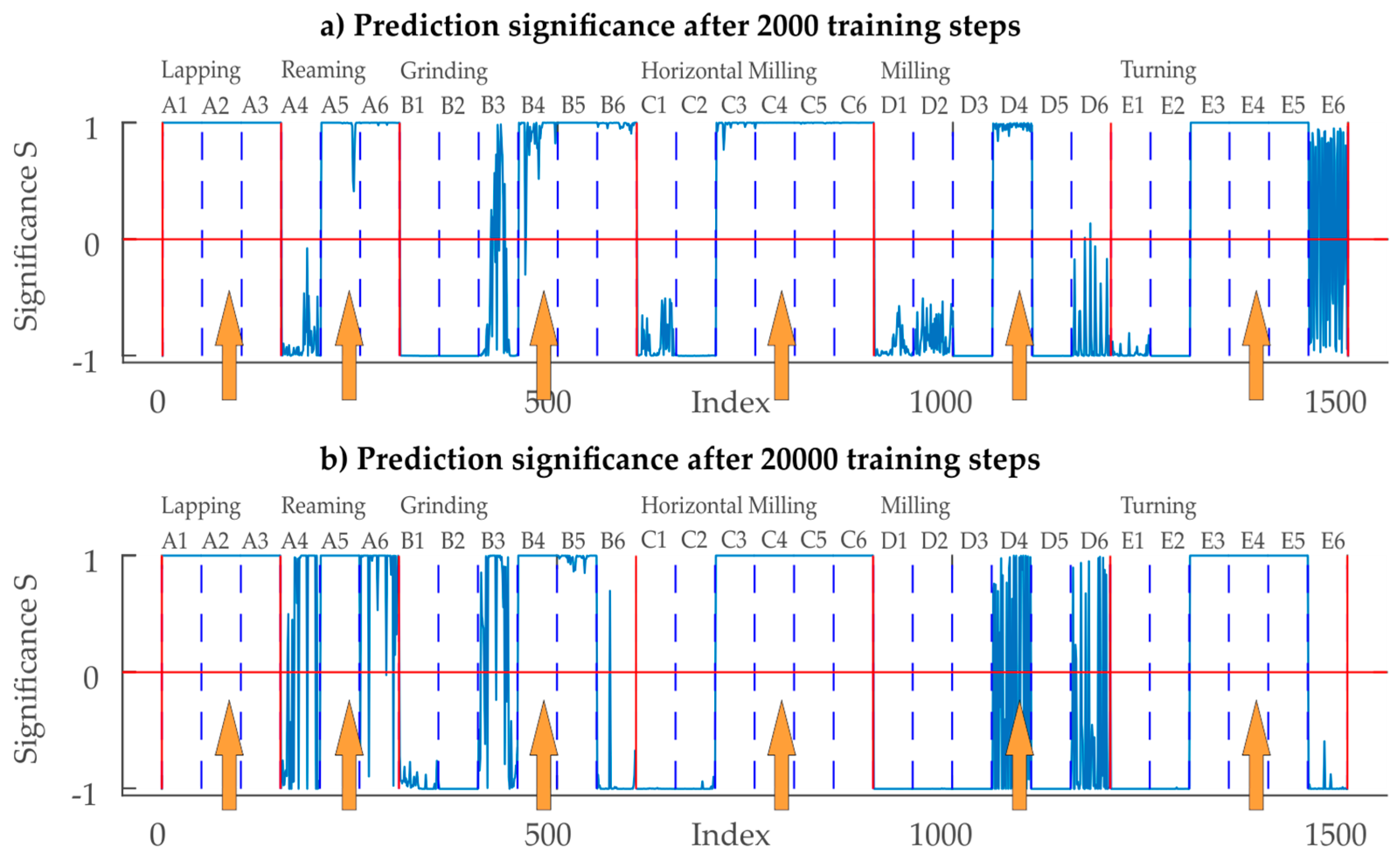
and Figure 10), and with increasing number of training steps (first and 2nd entry in each cell in Table 2). In order to quantify how distinct a classification is, a metric based on the output vector of the SoftMax layer for each sample is introduced. For the prediction significance $S$ (shown in Figure 10 and Figure 11) two cases are distinguished: If the input profile is classified correctly, the significance value $S$ of the $k$-th recognition is defined as the difference between the maximum of the SoftMax-vector and the 2nd largest value in the SoftMax-vector. Else, if the sample is classified incorrectly, the significance value $S$ is defined as the difference between the maximum of the SoftMax-vector and the prediction probability of the true class in the SoftMax-vector. Thus, with the given definition, the prediction significance provides a normalized measure between −1 and 1. A prediction significance of 1 means that the best possible prediction is present. A negative number indicates that the sample is incorrectly classified. An absolute value of $S$ close to zero indicates that the classification is ambiguous.

All three roughness degrees A1–A3 from the class Lapping were identified correctly (~100% performance) with a significance close to 1. For the class Reaming, only 24% of the samples A4–A6 are classified correctly after 2000 steps which increases to 51% after 20,000 training steps. Of all the classes, Reaming classification performed worst and solutions for a better distinction of reamed and milled surfaces are subject to future work. The significance of the prediction for Reaming increases with the number of training steps, meaning that after 20,000 steps, the significance is close to either +1 or −1. With fewer training steps, almost 60% of the Reaming data is misclassified as milled surfaces. This means that there are stochastic similarities between the two classes which should be examined further, especially since Grinding is not misclassified as Reaming. This decreases to 29% with the additional training. Another 16.67% is misclassified as Horizontal Milling, independent of the number of training steps. 62% and 96% of the grinding samples are correctly classified after 2000 and 20,000 steps respectively. 27% of the grinding samples are confused as Lapping samples (after 2000 steps), which decreases to 1% with additional training, thus resulting in the close to perfect classification performance. Horizontal Milling is correctly classified with a 68% and 76% percentage, with 14% of the data being confused as Reaming, independent of the amount of training. Initially 17% are confused as Grinding, which drops to 7% with additional training. Milling is a problematic type of surface for the CNN-classificator trained with artificial data: Only 59% and 43% are classified correctly (after 2000 and 20,000 steps), thus making Milling the only class whose classification performance dropped with additional training. Misclassified samples are confused as Turning surfaces with a probability of 27% and 31%. Turning is classified correctly for 100% of the data, independent of the training steps. When looking at the classification significance, an increased number of training steps not only results in more correctly classified samples, but also in higher significances.

5.3.2. Classification Performance with Reduced Set of Training Data

In Figure 11 the orange arrows indicate the selected profiles for the training data. Results for the CNN trained with only a part of the training data differ largely from the previous one: With 2000 training steps, an overall classification rate of 56% (mean of classification performance 61%) is achieved. This drops to 53% (mean of classification performance 59%) when training for 20,000 steps, which hints that training is completed after 2000 steps. The classification performance varies again between the classes (see

Table 3. Classification performance of the CNN trained with the reduced training set with actual measurement data after 2000 training steps (upper row) and 20,000 steps (lower row).

	Lapping as	Reaming as	Grinding as	Horizontal Milling as	Milling as	Turning as
Lapping in % (n)	100 (150)	0 (0)	46 (138)	8.33 (25)	0 (0)	0 (0)
	100 (150)	0 (0)	40.33 (121)	0 (0)	0 (0)	0 (0)
Reaming in % (n)	0 (0)	66.67 (100)	0 (0)	16.67 (50)	18 (54)	0 (0)
	0 (0)	83.33 (125)	16.33 (49)	16.67 (50)	50 (150)	0 (0)
Grinding in % (n)	0 (0)	33.33 (50)	54 (162)	8.33 (25)	32 (96)	33.33 (100)
	0 (0)	14 (21)	43.33 (130)	16.67 (50)	0 (0)	33.33 (50)
Horizontal Milling in % (n)	0 (0)	0 (0)	0 (0)	66.67 (200)	16 (48)	8 (24)
	0 (0)	2.67 (4)	0 (0)	66.67 (200)	11.33 (34)	16.67 (50)
Milling in % (n)	0 (0)	0 (0)	0 (0)	0 (0)	17.33 (52)	0 (0)
	0 (0)	0 (0)	0 (0)	0 (0)	12 (36)	0 (0)
Turning in % (n)	0 (0)	0 (0)	0 (0)	0 (0)	16.67 (50)	58.67 (176)
	0 (0)	0 (0)	0 (0)	0 (0)	26.67 (80)	50 (150)

and Figure 11): All three grades from the class Lapping were identified correctly (100% performance) when training for 2000/20,000 steps. This result is similar to the classification performance with the full training set, hinting that the identification of lapped surfaces is suitable for CNNs. For the class Reaming, 67% of the samples are classified correctly when training for 2000 steps. When looking at the significance one can see that two grades for Reaming are classified correctly (Figure 11, A5 & A6) while the finest Reaming grade (A4) is confused as Grinding. Further training (20,000 steps) increases the detection rate to 83%. The class Grinding is classified correctly in about 54% (43.33% for 20,000 training steps) of the samples, but also misclassified as Lapping in about another 46% (40% for 20,000 training steps) of the cases. The misclassified profiles are exclusively related to the finer Grinding samples (B1–B3). Both manufacturing principles generate surfaces that have a very stochastic character, which is an explanation for the wrong classifications. Horizontal Milling is correctly classified at a 67% (67%) rate for 2000 (20,000) training steps. The finer Horizontal Milling grades (C1 & C2) are problematic for classification since they are confused as Lapping (8%/0%), Reaming (17%/17%) and Grinding (8%/17%). Classification performance for the class Milling is worst with just 17% (12%), which might be related to the fact that this manufacturing principle features some stochastic as well as deterministic features. The class Turning is identified correctly in just above 59% (50%) of the cases. The misclassified samples in the class Horizontal Milling are mainly confused as Grinding, and Horizontal Milling. As the manufacturing principles Turning, Horizontal Milling and Milling all feature periodic deterministic structures, also in-between these classes, some wrong classifications can be expected.

In summary, only Milling (and Grinding after 20,000 training steps) was classified incorrectly by more than 50%. For five of six classes, application of the CNN-based classifier resulted in a better performance than a naïve guess. All the process-grades used for training data generation (indicated with an arrow in Figure 11) were identified close to 100% correctly. This shows that the character of the same machining process, but different roughness, differs considerably. Investigations of these scale effects and their consideration in the CNN are subject to future work. The generalization of the stochastic properties of a single evaluation area of one roughness degree to different process degrees is only valid for Lapping. Reaming, Grinding, Horizontal Milling, Turning and Milling showed problems in generalization, especially with the tending to finer grades. This means that the degree of roughness of these manufacturing principles has an influence on the stochastic properties of the surfaces.

However, with just one dataset of each manufacturing principle, a CNN could be trained that featured a recognition rate of approximately 60%. This means that based on this small database extracted from the ARMAsel approach, already an artificial neural network with classification performance close to 4× high than a naïve guess could be created, which is a promising result. A discussion and analysis of the weights in the CNN is omitted, since the visual interoperation of the weights is not possible. The next step in the classification process is to apply the obtained classifier to a larger number of different technical surfaces and samples in order to check whether a similar classification rate can be achieved. To use and distribute the system successfully, a classification rate of about 90% is desirable. Thus for the required enhancement of the classification rate, both the approach for data generation and the structure of the CNN are subject to future improvement. One approach can be the transformation of the surfaces from spatial to frequency domain and training of the classifier based on the PSD. Also a combined approach using both the spatial and frequency domain as input data is possible.

6. Conclusions

A routine was examined to determine the best possible time series model for the description of rough surfaces. With this model, the PSD and ACF of the surface could be calculated and the determined coefficients of the times series models were used as input data for the generation of artificial surfaces with desired stochastic properties.

This can enhance a previously described method [7] for training classifiers of ANNs: in order to generate more realistic training data for the ANN, surface profiles of various manufacturing principles were generated based on actual measurement data, without the requirement for manual input. Based on the ARMAsel algorithm [26], a systematic investigation of the description of rough surfaces with the aid of time series models was conducted. This was done by examining a broad range of surface types. In doing so, the chosen models, their number of parameters and the resulting prediction errors were determined at different evaluation positions. The AR-model and ARMA-model most often lead to the smallest prediction error, the MA-model leads to similar results for some surfaces and is best suitable for the description of fine, stochastic surfaces.

Regarding the description of rough surfaces with time series models, the following conclusions were drawn: for the required number of parameters, the complexity of the roughness structure is the most relevant influence. Moreover, for most surface types, finer surfaces require more parameters as more frequencies are present. More stochastic profiles usually obtain a reduced number of parameters in comparison to deterministic profiles. When the quality of the models is estimated, the best results were achieved for stochastic surfaces. Surfaces which feature deterministic patterns caused by the manufacturing process could not be fully described with the proposed stochastic models, required more coefficients and exhibited a higher difference between the PSDs extracted from the profile and the coefficients.

Based on the calculated AR-, MA- and ARMA-models an improved generation of artificial technical surfaces compared to previous work [7] was proposed. In doing so, the stochastic profile data was obtained from measured datasets. The described method can assist in an automated recognition of manufacturing principles of technical surfaces which can support the operators of measuring instruments in the evaluation process with suggestions for evaluation parameters. With only one 4 mm profile extract for each class of all manufacturing principles and the according ARMA-coefficients, training data for a CNN was generated which was able to determine the manufacturing principle of actual measurement data with a rate of approximately 78%. Thus, much stochastic surface information of various manufacturing principles was obtained with only very few measured data.

The classification performance dropped to about 60% when only one sample per class was used for data simulation, which is still about 4× higher than a naïve classifier. The Lapping processes were recognized reliably for varying degrees of roughness. Other manufacturing principles indicated a variation of the stochastic properties with the degree of roughness.

With the given results, it was shown that the ARMAsel approach can be used to extract the stochastic information of varying technical surfaces. This information allows a reliable artificial surface data generation. The resulting simulated profiles were used for training classifiers that achieved a high recognition rate and can serve as a framework for an automated determination of surface evaluation parameters. One current drawback is the lack of a larger validation set of independent test samples for classification. Thus, the current approach should be validated with a broader data base.

In upcoming studies, surfaces which feature deterministic and long-wave structures should be examined more in depth. As areal surface topography measurement is a subject of growing interest, the stochastic properties of 3D-topographies should as well be examined by an extension of the proposed methods.