A Novel Kernel-Based Regularization Technique for PET Image Reconstruction

Abstract

Positron emission tomography (PET) is an imaging technique that generates 3D detail of physiological processes at the cellular level. The technique requires a radioactive tracer, which decays and releases a positron that collides with an electron; consequently, annihilation photons are emitted, which can be measured. The purpose of PET is to use the measurement of photons to reconstruct the distribution of radioisotopes in the body. Currently, PET is undergoing a revamp, with advancements in data measurement instruments and the computing methods used to create the images. These computer methods are required to solve the inverse problem of “image reconstruction from projection”. This paper proposes a novel kernel-based regularization technique for maximum-likelihood expectation-maximization ($\kappa$-MLEM) to reconstruct the image. Compared to standard MLEM, the proposed algorithm is more robust and is more effective in removing background noise, whilst preserving the edges; this suppresses image artifacts, such as out-of-focus slice blur.

1. Introduction

Efforts are underway to improve the image reconstruction quality achieved by positron emission tomography (PET) [1]. The purpose of PET is to provide 3D imaging of the administered tracer distribution, which is believed to be associated with the distribution of activity of certain molecular mechanisms underlying pathology or disease models [2]. More detailed PET scans require the injection of a small amount of biologically-relevant material, such as glucose or oxygen, that has marked radionuclides [3]. All of the isotopes used are radioactive with a rapid decomposition time by positron emission. The most common isotope employed in PET is fluorine-18 [4]. This tracer is very useful because of its long half-life (110 min) and because it disintegrates by emitting positrons having a low positron energy that contributes to high-resolution imaging acquisition. The molecule accumulates in cells that are most metabolically active, or if the molecule is receptor-specific, it collects in cells where the receptors are present. This evaluation of the cellular and physiological function by nuclear medicine can be effectively used to locate and determine the extent of a disease in the body. Nowadays, a major set of PET applications is in oncology [5], cardiac imaging [6], and brain imaging [7]. With the developments of specific radiotracers, several applications of PET in neurology have been found during the last few years, such as dopamine neurotransmitter imaging in Parkinson’s disease and tau imaging [8] in Alzheimer’s disease. PET works by a radioactive tracer that has been introduced into the body, decaying to emit a positron $\beta +$, which can only travel a few millimeters (the positron range [9]), before colliding with an electron. The antimatter–matter collision annihilates both particles and results in a pair of 511-keV gamma photons that travel in nearly opposite directions. A pair of detectors is connected by a line of response (LOR) and is tuned to pick up photons within a coincidence-timing window.

The annihilation events can be stored in list-mode format or in a 3D matrix according to the position of their corresponding line of response. The process of acquiring the projection data is called emission scan. The histogram data are said to lie in a sinogram or projection domain, and the object to be scanned is said to lie in an image domain. The emission tomography uses the projection data to reconstruct the spatial distribution of the radioisotope by taking into account the geometric factors, noise properties, and physical effects. To estimate the radioactivity distribution accurately, we must consider the effects of the attenuation that result from the photoelectric absorption effects as a consequence of the interaction of the emitted gamma photons through the subject matter and the gantry.

The PET image is reconstructed from the acquired projection data, but as the count of the projection data declines, there is an increase in noise in the reconstructed PET image. The most simple method used to reconstruct the PET image is the analytical method called filtered back-projection (FBP) [10]. Yet, because of the Poisson-distributed noise that is characteristic of projection data, FBP-reconstructed PET images are often of low quality. Alongside regular reconstruction methods, noise smoothing can be performed in the pre-reconstruction phase of the sinogram domain [11,12,13,14,15], in the post-reconstruction phase of the image [16,17,18], or during the iterative process of statistically-based reconstruction [19]. An alternative method that incorporates prior knowledge into de-noising images is non-local means (NLM) [20,21]. In general, applying denoising methods correctly and accurately post-reconstruction is more difficult than within the reconstruction.

This paper uses the maximum-likelihood expectation-maximization (MLEM) algorithm to reconstruct PET images [22,23]. Using MLEM for PET image reconstruction that has a noisy dataset results in a noisy image. Therefore, to improve the quality of the image, we propose a novel kernel-based image regularization technique. Of the various possible options of the kernel function, an exponentially-modified Gaussian kernel was used [24,25,26]; this is comparable to conventional MLEM reconstruction in terms of simplicity. Noise is modeled in the projection domain, where independent Poisson random variables effectively model the PET data. The results indicated that the proposed kernel-based MLEM ($\kappa$-MLEM) method provides effective reconstruction and resolution results that exceed those generated by conventional MLEM and advanced pre-reconstruction methods.

In Section 2 of this paper, the novel MLEM kernel-based regularization image reconstruction method is outlined. Section 3 presents the PET setup and the evaluation criteria for the quality of the reconstruction. Results are presented in Section 4, together with a comparison of the $\kappa$-MLEM and other methods. Section 5 is the conclusion.

2. Materials and Methods

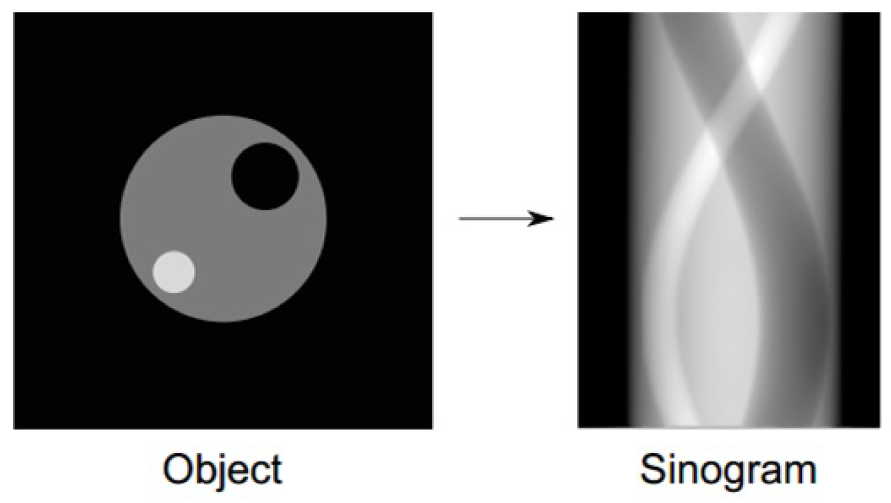
2.1. Data Acquisitions and Sinograms

PET scans detect vast numbers of pairs of annihilation photons. The total number of pairs of photons measured by a particular detector pair is proportional to the integrated radioactivity that occurs along the line joining the detector pair. LORs pass through a single point in the patient body and trace a sinusoid curve in the raw data histogram; hence the term sinogram for the raw data format. A simple example of an object in the spatial domain and its corresponding sinogram are illustrated in Figure 1.

2.2. PET Data Corrections

Collecting PET data is not a perfect process. The photons emitted within the patient are attenuated by photoelectric interactions; the efficiency of detector elements is variable, and together with recording true coincidence events, random and scattered coincidences are accrued. To create a clinically-valuable image and reliable quantitative information, these artifacts and errors need to be corrected.

Attenuation correction (AC) is the most important data adjustment [27]. The effect of encountering dense or a greater quantity of material on the path between the annihilation site and the detector leads to photon absorption or scattering. The result is an attenuation of photons in those environments compared to photons that do not encounter such material. Images that are reconstructed from projection data of photons in less dense areas of the body (e.g., the lungs) appear dark, as they have emitted more photons than the surrounding tissue (e.g., the mediastinum), which is dense.

Random coincidences are also corrected [28]. These need to be estimated and minimized from the collected measurements in each LOR to find the sum of scattered and true coincidences, which is necessary for quantitative measurement.

2.3. Maximum-Likelihood Expectation-Maximization Algorithm

Following the acquisition and correction of PET data in the sinograms, an estimate of the in vivo tracer distribution needs to be determined. This is a mathematically complex stage, and is covered in detail in [29,30,31]. It is assumed that the object being imaged has a radionuclide distribution represented by the matrix $x_j$, where the index j denotes the location of an individual volume element (“voxel”) in the object.

The purpose of the tomographic reconstruction algorithm is to calculate the radionuclide image $x_j$ from the set of counts $b_i$ recorded by the external detector array circling the patient, where the index i identifies the position of each detector element used in making our measurement from the patient. In this mathematical derivation, the radionuclide image $x_j$ is represented as a matrix in which each matrix element $x_j$ represents the radionuclide concentration at a point identified by the index j. Similarly, the recorded radionuclide projection data $b_i$ are represented as a matrix, in which each matrix element $b_i$ identifies both the angle and the location of the detector, where the data are recorded.

We assume that we know the probability $P_{ij}$ of a photon emitted in voxel j being detected by detector i. The value of the detection probability $P_{ij}$ is directed by physical phenomena, such as the geometric efficiency of the collimator, the attenuation provided by the material surrounding the radioactive voxel j, and the detection efficiency of the imaging system.

The behavior of the imaging system can be represented by using a matrix equation that couples the radionuclide concentration $x_j$ in the object to the complete set of detector measurements $b_i$ using the known value of the probability elements $P_{ij}$:

$$\left[\begin{array}{c}{b}_1\\ b_2\\ \cdots \\ b_i\\ \cdots \\ b_M\end{array}\right]=\left[\begin{array}{cccccc}{P}_{11}& P_{12}& \cdots & P_{1j}& \cdots & P_{1N}\\ P_{21}& P_{22}& \cdots & P_{2j}& \cdots & P_{2N}\\ \cdots & \cdots & \cdots & \cdots & \cdots & \cdots \\ P_{i1}& P_{i2}& \cdots & P_{ij}& \cdots & P_{MN}\\ \cdots & \cdots & \cdots & \cdots & \cdots & \cdots \\ P_{M1}& P_{M2}& \cdots & P_{Mj}& \cdots & P_{MN}\end{array}\right]·\left[\begin{array}{c}{x}_1\\ x_2\\ \cdots \\ x_j\\ \cdots \\ x_N\end{array}\right]$$

(1)

As the values of $b_i$ can be measured with the detector array and since the value of the probability elements $P_{ij}$ can be calculated from the physics of the imaging system, the matrix equation Equation (1) can be mathematically inverted to solve for the radionuclide distribution $x_j$. In reference to matrix Equation (1), the radionuclide concentration $x_j$ is unknown, but a solution can be assumed. Consequently, $x_j$ is the best estimate of the true radionuclide distribution.

Since the probability matrix $P_{ij}$ is known, it is possible to estimate the detector counts ($b_i$) that would be obtained for the estimated radionuclide distribution $x_j$ using the forward projection operation:

$$b_i=\sum _{j=1}^N{P}_{ij}{x}_j$$

(2)

Reconstruction is primarily founded on a mathematical model that relates parameters to the observed and unobserved data. The mathematical model is based on the notion that emissions occur according to a spatial Poisson point process inside the region of interest in the source. For each detector position i, the appropriate model is a Poisson-distributed random variable $b_i$ [22]. The probability matrix $P_{ij}$ is known from the detector array geometry, the attenuation provided by the material system and the detection efficiency of the imaging system. Suppose $y_i$ is the expected values of Poisson-distributed random variables $b_i$ where:

$$P\left(b_i\right|y_i)=e^{-y_i}\frac{{\left(y_i\right)}^{b_i}}{b_i!}$$

(3)

The expectation of the detected data is combined with the model parameters:

$$y_i=E\left[b_i\right]=\sum _{j=1}^N{x}_j{P}_{ij}$$

(4)

Since the variables ${\lambda }_{ij}$—the number of emissions in voxel j detected in detector i—are independent Poisson-distributed random variables with the mean,

$$E\left[{\lambda }_{ij}\right]=x_j{P}_{ij},$$

(5)

the likelihood function is then:

$$L\left(x\right)=\prod _{j=1}^N\prod _{i=1}^M{e}^{-x_{ij}}\frac{{\left(x_{ij}\right)}^{{\lambda }_{ij}}}{{\lambda }_{ij}!}$$

(6)

Although the sum in (6) is complicated, it shows that the log-likelihood is concave as a function of x:

$$l\left(x\right)=logL\left(x\right)=\prod _{j=1}^N\prod _{i=1}^M-x_j{P}_{ij}+{\lambda }_{ij}log{x}_j+{\lambda }_{ij}log{P}_{ij}-log{\lambda }_{ij}!$$

(7)

The E-step is computed as:

$${\lambda }_{ij}^{[k+1]}=E[{\lambda }_{ij}|b_i,x^{\left[k\right]}]$$

(8)

Since we know that ${\lambda }_{ij}$ are Poisson-distributed random variables with mean $x_{ij}^{\left[k\right]}$ and $b_i={\sum }_{j=1}^N{\lambda }_{ij}$, also Poisson with mean $y_i^{\left[k\right]}={\sum }_{j=1}^N{x}_{ij}^{\left[k\right]}$, after some manipulations:

$${\lambda }_{ij}^{[k+1]}=\frac{b_i{x}_{db}^{\left[k\right]}}{{\sum }_{\acute{j}=1}^N{x}_{i\acute{j}}^{\left[k\right]}},j=1,2,\cdots ,N;i=1,2,\cdots ,M$$

(9)

In the M-step, we maximize

$$\begin{array}{c}0=\frac{\partial }{\partial x_j}\sum _{j=1}^N\sum _{i=1}^M-x_j{P}_{ij}+{\lambda }_{ij}^{[k+1]}log{x}_j+{\lambda }_{ij}^{[k+1]}log{P}_{ij}-log{\lambda }_{db}^{[k+1]}!\hfill \\ \hfill & \hfill \to x_j^{[k+1]}=\sum _{i=1}^M{\lambda }_{ij}^{[k+1]}{P}_{ij}\end{array}$$

(10)

Combining the E and the M steps:

We start the algorithm with an initial guess $x_j^{\left[0\right]}$, and then, in each iteration, if $x_j^{\left[k\right]}$ denotes the current estimate of $x_j$, the new estimate is defined as:

$$x_j^{[k+1]}=x_j^{\left[k\right]}\sum _{i=1}^M\frac{b_i{P}_{ij}}{{\sum }_{\acute{j}=1}^N{x}_{\acute{j}}^{\left[k\right]}{P}_{i\acute{j}}}$$

(11)

The MLEM algorithm is summarized as:

• Start with an initial estimate $x_j^{\left[0\right]}$ satisfying $x_j^{\left[0\right]}>0,j=1,2,\cdots N$,
• If $x_j^{\left[k\right]}$ denotes the estimate of $x_j$ at the $k^{\mathrm{th}}$ iteration, define a new estimate $x_j^{[k+1]}$ by using Equation (11),
• If the required accuracy for the numerical convergence has been achieved, then stop.

2.4. Regularization

The expectation maximization algorithm is ill-conditioned, which means that enforcing the maximization of the likelihood function may result in a solution with severe oscillations and noisy behavior.

2.4.1. The Non-Local Means Filter

The $NLM$ algorithm is a nonlinear spatial filter that uses a weighted average of the intensity of adjacent pixels to adjust the intensity value of each pixel [20,21]. While comparisons of neighboring pixels can be performed between pixels separated in the image by any distance, for the benefit of computation speed, comparisons are typically limited to a narrow search window around the pixel undergoing value adjustment.

Mathematically, this method can be described as:

$$y\left[k\right]=\frac{1}{C_N}\sum _{n\in SW}W[k-n]·x[k-n]$$

(12)

where $y\left[k\right]$ is the new pixel value at coordinate k, $C_N$ is a normalization constant, $SW$ is the search window centered at k, $x[k-n]$ is the original pixel value at the ($k-n$) coordinate within the search window, and $W[k-n]$ is the weight given the intensity value of $x[k-n]$. The weights are calculated as:

$$W[k-n]=exp(-\sum _{m\in P}{K}_G{[\frac{x[k-m]-x\left[\right(k-n)-m]}{h}]}^2)$$

(13)

where P is the patch size around each pixel that is being compared, $K_G$ is a Gaussian kernel used to reduce the weight in the similarity calculation given to patch pixels further from the center, and h adjusts the intensity similarity-to-weight relationship.

2.4.2. The Anisotropic filtering

The anisotropic filter ($AF$) attempts to avoid the blurring effect of the Gaussian by convolving the image x at j only in the direction orthogonal to $Dx\left(j\right)$. The idea of such a filter goes back to [32]. It is defined by:

$$A{F}_{h}x\left(j\right)=\int G_h\left(t\right)x(j+t\frac{Dx{\left(j\right)}^{\perp }}{\left|Dx\right(j\left)\right|})dt$$

(14)

for j such that $Dx\left(j\right)\ne 0$ and where ${(j,l)}^{\perp }=(-l,j)$ and $G_h$ is the one-dimensional Gaussian function with variance $h^2$. The image method noise of an anisotropic filter $A{F}_h$ [20] is $x\left(j\right)-A{F}_{h}x\left(j\right)=-\frac{1}{2}{h}^2\left|Dx\right|curv\left(x\right)\left(j\right)+o\left(h^2\right)$, where h is a filtering parameter (which usually depends on the standard deviation of the noise), and $curv\left(x\right)\left(j\right)$ denotes the curvature, the signed inverse of the radius of curvature of the level line passing by j. This method noise is zero wherever x behaves locally like a straight line and large in curved edges or texture. Consequently, the straight edges are well restored, while flat and textured regions are degraded.

An extended discussion of the anisotropic filter for attenuation correction in PET can be found in [11].

2.4.3. Proposed Kernel-Based Exponentially-Modified Gaussian Regularization

Inspired by the kernel-based image representation for PET images [25], we propose a new kernel-based image regularization technique to improve the PET image reconstruction. We define $x_j$ as a feature map for pixel j that is the output of the kernel, which is a mixture of two sets of information. The first set is the input image, which has a matrix of pixels, where a pixel consists of an integer value between zero and 80. The second set is the convolution kernel, which consists of a single matrix of floating point numbers.

Convolution can be considered a mixing of information. This is achieved by taking an image box from the input image that is the size of the kernel. This experiment uses a $256\times 256$ image and a $7\times 7$ kernel, so it would take $7\times 7$ boxes. An element-wise multiplication with the image box and convolution kernel is performed, and the sum of this multiplication results in a single pixel of the feature map, as depicted in Figure 2, by using a $3\times 3$ kernel.

The image intensity at pixel j is represented by a linear combination of the kernels,

$$x_j=\sum _{l=1}^N\kappa (j,l)·{\chi }_l$$

(15)

where N is the total number of pixels in the image and $\chi$ is the kernel coefficient image. $\kappa (·,·)$ is a kernel function encoding image prior information.

$$x=K\chi$$

(16)

In Equation (16), each column of K can be considered as a basis function for image representation. We proposed to use kernels including the exponentially-modified Gaussian [33]:

$$\kappa (x;\mu ,\sigma ,\delta )=\frac{\delta }{2}{e}^{\frac{\delta }{2}(2\mu +\delta {\sigma }^2-2x)}erfc(\frac{\mu +\delta {\sigma }^2-x}{\sqrt{2}\sigma })$$

(17)

where erfc is the complementary error function, defined as erfc$\left(x\right)=\left(2\sqrt{\pi }\right)·{\int }_x^{\infty }{e}^{-t^2}dt$, and $\sigma$, $\mu$, and $\delta$ are the kernel parameters in the respective kernels.

In most instances, the kernel in the image is center-originated, indicating that the center point of a kernel is $\kappa (0,0)$. For example, if the kernel size is five, then the array index of five elements will be $-2$, $-1$, 0, 1, and 2. The origin is located at the middle of the kernel.

Because PET projection data $b_i$ are well modeled as independent Poisson random variables with the log-likelihood function [34], the expectation $E\left[b_i\right]$ can be related to the unknown emission image $x_j$ through:

$$y_i=E\left[b_i\right]=\sum _{j=1}^N{x}_j{P}_{ij}+r$$

(18)

with P being the detection probability matrix and r the expectation of random and scattered events. Substituting Equation (16) into (18), we obtain the following kernel-based forward projection model:

$$E\left[b_i\right]=\sum _{j=1}^{N}K{\chi }_j{P}_{ij}+r$$

(19)

Combining the kernel-based projection model and the standard MLEM algorithm [22] given in Equation (11), it can be directly applied to find the $ML$ estimate of $\chi$ because of (20). The resulting kernelized EM update of $\chi$ at iteration ($k+1$) is:

$${\chi }_j^{[k+1]}=K{\chi }_j^{\left[k\right]}\sum _{i=1}^M\frac{b_i{P}_{ij}}{{\sum }_{j^{\prime }=1}^{N}K{P}_{i{j}^{\prime }}{\chi }_{j^{\prime }}^{\left[k\right]}+r}$$

(20)

3. Computer Simulation

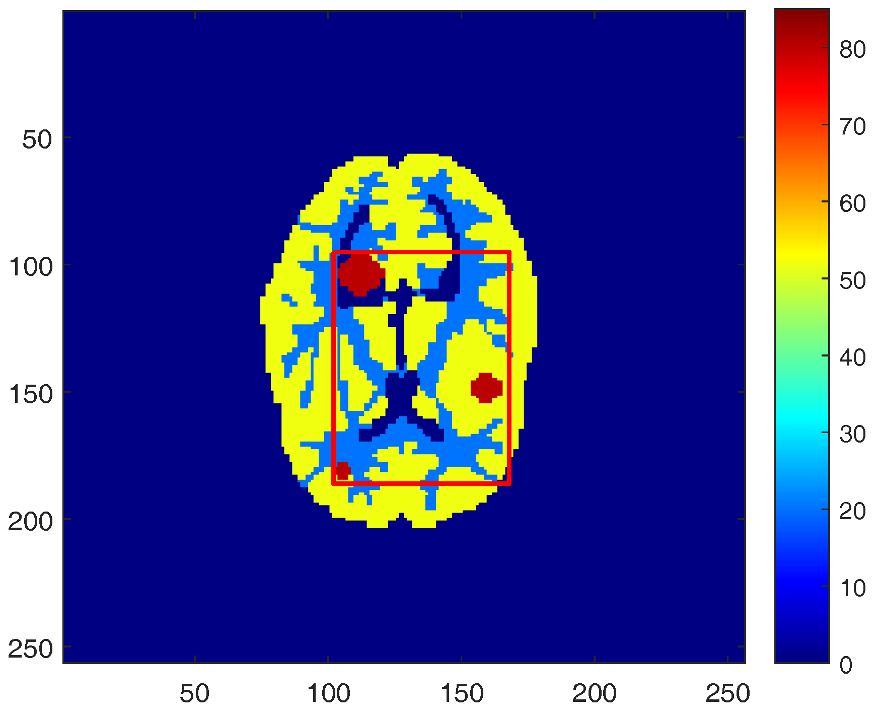
3.1. Simulated PET Data (Setup)

To assess the overall performance of the proposed kernel regularization algorithm, we simulated a PET scanner in a 2D mode, which has 420 crystals in each ring with each crystal having a cross-section of $6.3\times 6.3{\mathrm{mm}}^2$. A Hoffman brain phantom (Figure 3) [35] was used to simulate the radioactivity distribution in a single slice of PET tracer through grey matter, white matter, and three tumors. The digital design of the tumors in the phantom provides essential information about the reconstructed images. To create a projection data, the simulated phantom image was forward projected using the system matrix to generate the noise-free projection data. Once the simulated noise-free sinograms were produced, a $30\%$ uniform background was added to simulate mean randoms and scatters. The fraction of random and scatter was determined by counting them and dividing them by the total number of counts. Independent Poisson noise was then introduced to the projection data with the expected total number of events set to $300$k. All images were represented by $256\times 256$ pixels with a pixel size of $3\times 3{\mathrm{mm}}^2$. All of the codes in the following experiments are implemented in MATLAB R2013a and run on a desktop computer with i5-6600 @ 3.30 GHz 3.31 GHz Intel Core CPU and 8 GB memory.

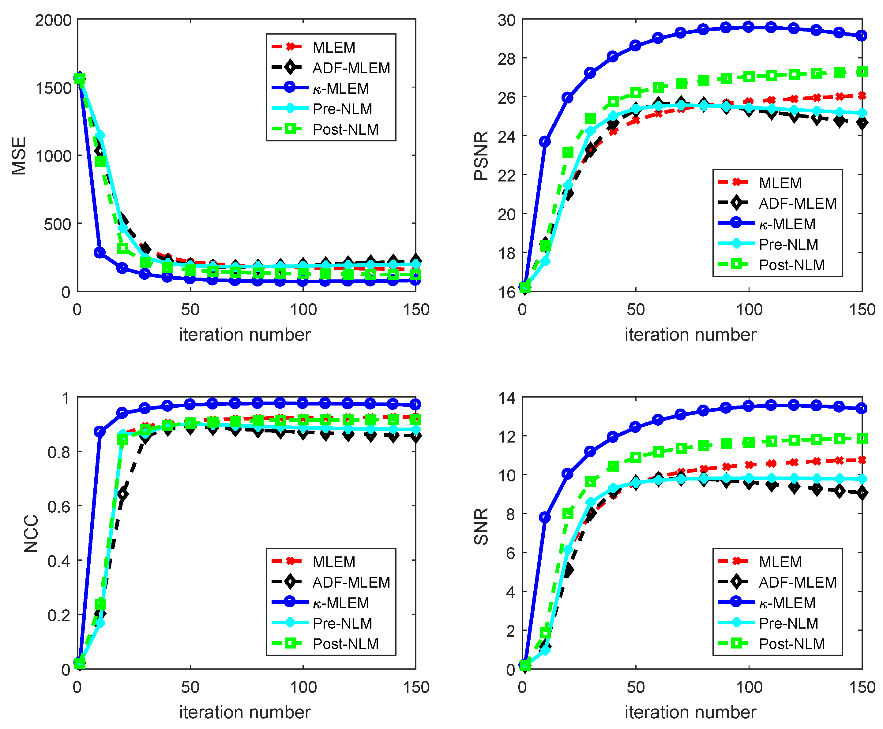
3.2. Quality Evaluation

To evaluate the reconstructed results objectively, four image quality measurement parameters were computed. These are listed below.

The mean square error is defined as [36]:

$$MSE=\frac{1}{MN}\sum _{j=1}^M\sum _{i=1}^N{(x_{j,i}-x_{j,i}^{\prime })}^2$$

(21)

The peak signal-to-noise ratio is defined as [37]:

$$PSNR=10log\frac{{255}^2}{MSE}$$

(22)

The signal-to-noise ratio is defined as [38]:

$$SNR=\frac{{\sum }_{j=1}^M{\sum }_{i=1}^N{[x_{j,i}^{\prime }]}^2}{{\sum }_{j=1}^M{\sum }_{i=1}^N{[x_{j,i}-x_{j,i}^{\prime }]}^2}$$

(23)

Normalized cross-correlation is defined as [39]:

$$NCC=\frac{{\sum }_{j=1}^M{\sum }_{i=1}^N(x_{j,i}{x}_{j,i}^{\prime })}{{\sum }_{j=1}^M{\sum }_{i=1}^N{x}_{j,i}^2}$$

(24)

The test image’s grey level value is denoted by x, with $x^{\prime }$ being the same value in the reconstructed image. The lower MSE and greater PSNR, SNR, and normalized cross-correlation (NCC) values indicate that the resulting reconstructed image is closer to the test image. The iteration number is a further criterion that contributes to the iterative reconstruction algorithm, with smaller iterations being preferable. Filled contour plots displaying isolines of the reconstructed images and the plot of the profiles of reconstructed images’ comparisons were also used.

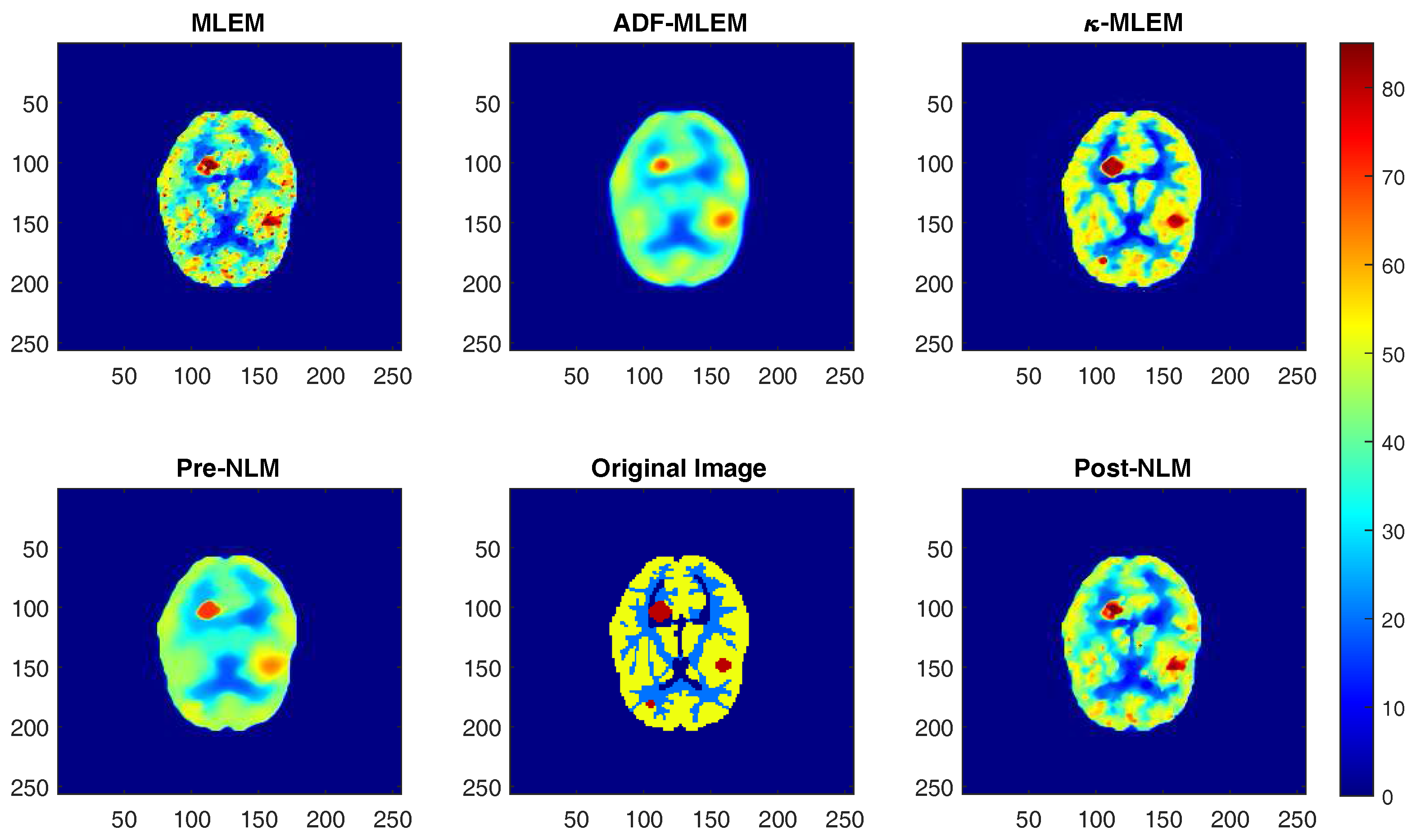
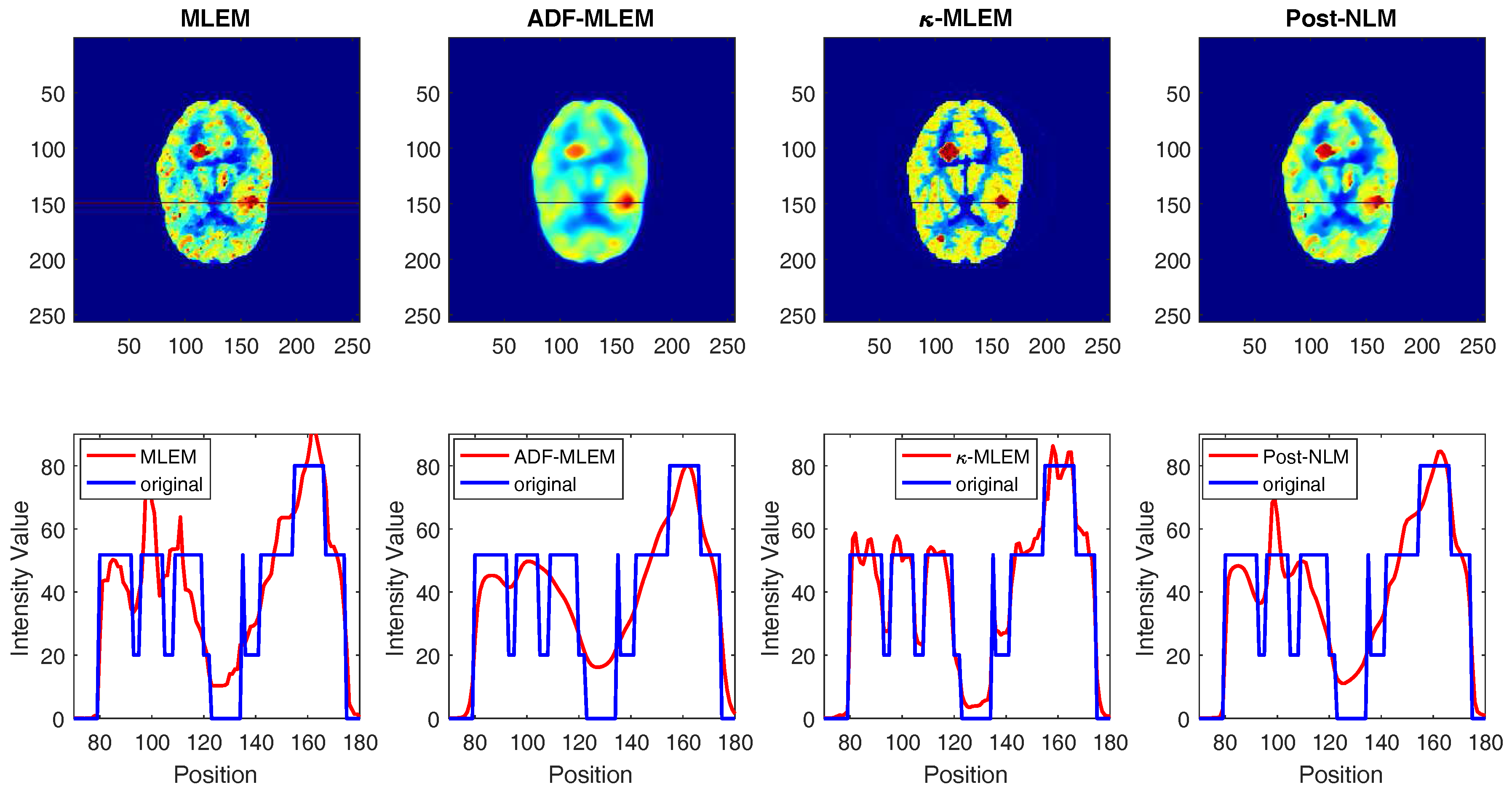
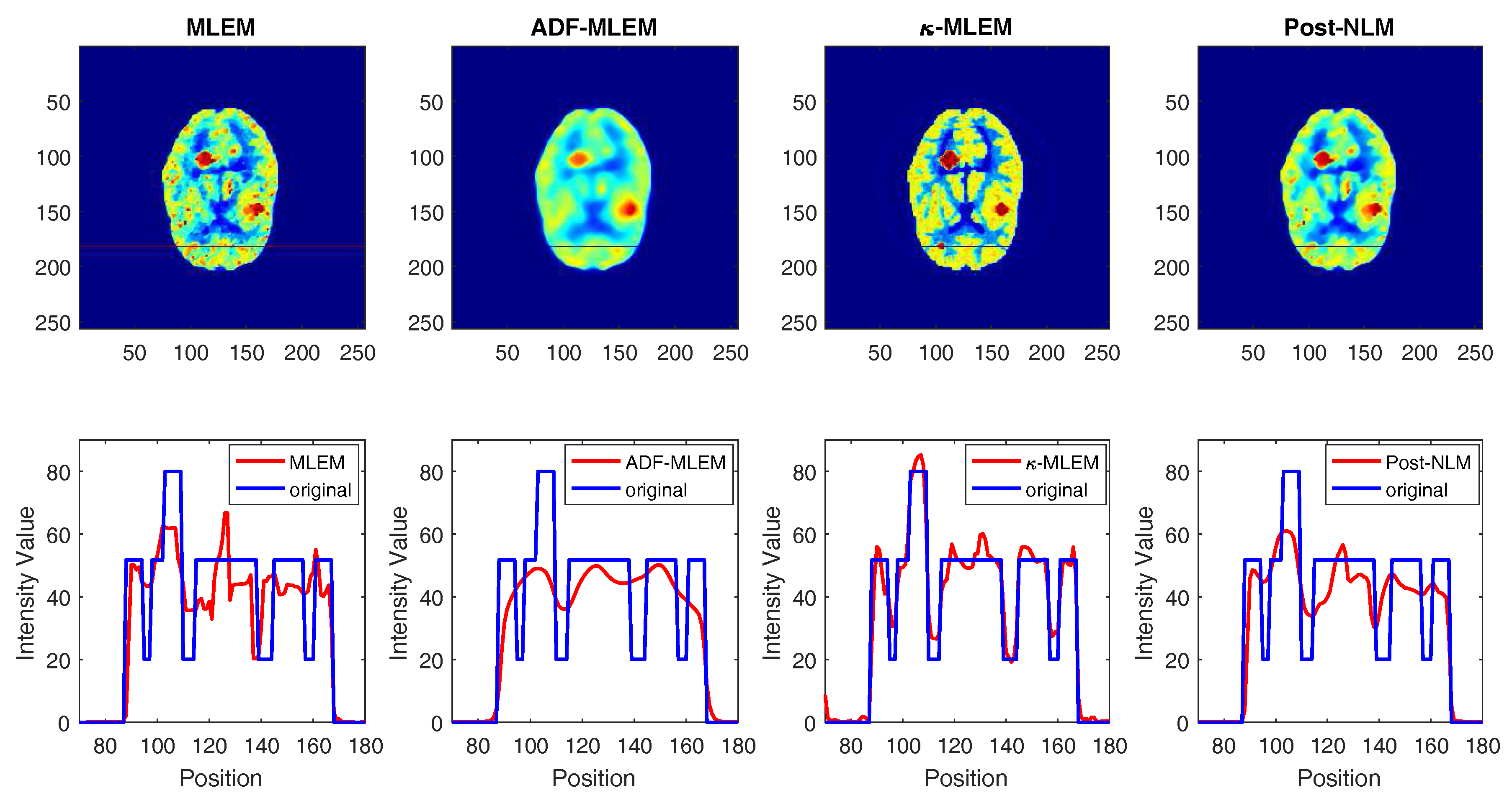
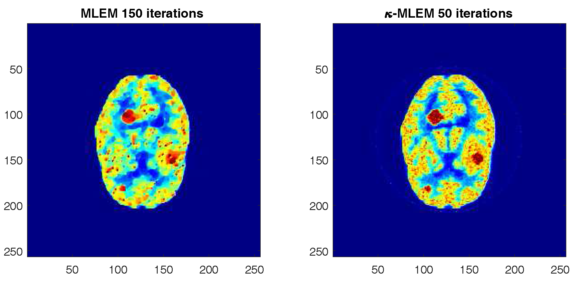
4. Results and Discussion

In this study, the experimental kernel-based MLEM ($\kappa$-MLEM) algorithm was compared against conventional MLEM [22], the penalized likelihood reconstruction regularized by anisotropic diffusion filter (ADF) [17], the MLEM precondition reconstruction algorithm that was regularized by non-local means (pre-NLM) and post-reconstruction de-noising methods applied post-MLEM (post-NLM) [20]. One hundred and fifty iterations were applied to the MLEM algorithm used in each of the regularization-based methods. Apart from the conventional MLEM algorithm, spatial smoothing was used to enhance the quality of the image. All images were sized at $256\times 256$ pixels. The box and neighborhood size were $7\times 7$.

We applied our technique to the Hoffman brain phantom, reconstructing the phantom erroneous projections. Figure 4 shows the reconstructed images.

As is shown, the visual quality of the reconstructed image of the phantom using the $\kappa$-MLEM algorithm is comparable to the other methods. Indeed, compared to some, the experimental algorithm preserves edges better. There is less noisy projection data, and the reconstruction is more accurate. The method was able to detect the three tumors of different sizes, the smallest of which was not picked up by ADF and pre-NLM and only faint in the post-NLM and conventional MLEM images. Sensitive and reliable visualization of brain tumors is important for medical diagnosis and prognosis.

The effectiveness of noise removal for the test algorithm was comparable to that of the post-NLM method; however, the intensity in the region of interest was appreciably higher in the latter. Compared to the other methods, the $\kappa$-MLEM method generates a superior intensity profile, whilst preserving the edges.

The SNR, MSE, PSNR, and NCC quality measurements of the reconstructed images derived from the proposed algorithm and the other four reconstruction algorithms for the tumor regions of interest (ROIs) of the Hoffman brain phantom selected with a rectangle in (Figure 3) are shown in Figure 5. The minimum MSE achieved by all of the different methods for all iterations are shown Figure 5a. The peak signal-to-noise ratio (PSNR) for each iteration is presented in Figure 5b. The normalized cross-correlation (NCC) and the signal-to-noise ratio values are shown in Figure 5c,d, respectively. These data indicate that the measurements provided by $\kappa$-MLEM are of a higher quality than the other methods tested. Compared to the performance parameters of the other regularization methods, those of the proposed method were enhanced—especially at the lower number of iterations—and remained almost constant after 100 iterations; for the conventional ADF-MLEM and pre-NLM, however, the performance parameters began to decrease after 80 iterations. The data presented in these images indicate that the $\kappa$-MLEM-generated images have the highest PSNR, SNR, and NCC at all iterations and have a lower MSE; thus, the method outperforms the other methods, and this effect is heightened as the iterations increase. We can see the post-NLM algorithm is clearly demonstrating a better performance than all of the other alternative techniques and a performance quite close to the $\kappa$-MLEM method. Indeed, the quality measurements of conventional MLEM at 150 iterations are not dissimilar to those of $\kappa$-MLEM at 50 iterations (Figure 6). The lowest threshold number of iterations the technique needs to create an acceptable reconstructed image is 20, making it fast as well as efficient. $\kappa$-MLEM is also effective in removing star artifacts that are commonly generated by the conventional MLEM algorithm.

The 1D line profile is the horizontal line that crosses the image in the two tumors, as shown in Figure 7 for the middle tumor and in Figure 8 for the small tumor. Noisy images in uniform regions are shown as spikes, as indicated by the conventional MLEM and post-NLM images; on the other hand, $\kappa$-MLEM line profiles are closer to being noise-free. The experimental method also nullifies aerial pixels, redistributing their values to pixels within the phantom. $\kappa$-MLEM reconstructed the ideal profile more effectively than the other methods, and the image produced was a close approximation of the original phantom image.

To evaluate the performance of our proposed algorithm in the detection of tumors, we compare the size of tumors of the original phantom and tumors of reconstructed images from different algorithms. The reconstruction outcomes of the simulated phantom yielded the two rectangular areas in Figure 9, which highlight the two smaller tumors. Subsequently, we used a threshold equal to $75\%$ to segment the tumors in PET images. The proposed algorithm successfully preserved the edges of tumors. For example, the middle tumor edges were effectively preserved when applying the proposed algorithm, whereas artifacts and deviations were more likely to occur with the NLM-MLEM and conventional MLEM algorithm and appear distorted with the ADF-MLEM algorithm, as shown in Figure 9. Furthermore, the intensity distribution within the middle tumor was made more homogeneous by the proposed algorithm as compared to the conventional MLEM algorithm. In addition to this, the proposed algorithm could enable the detection of the small tumor with the same size of the original tumor, unlike other algorithms, which did not show tumors at all.

5. Conclusions

The new reconstruction algorithm presented in this paper aims to improve the noise in PET images. Based on conventional MLEM, the experimental algorithm uses a box-kernel of the exponentially-modified Gaussian. The kernelized image model can incorporate prior information in the forward projection model $\kappa$-MLEM. The achievements of $\kappa$-MLEM were quantitatively superior, and there was a significant reduction in noise at matched contrast when tested against conventional MLEM and NLM regularization-based methods in PET simulations. Promising results were also achieved when the algorithm was used to reconstruct a Hoffman phantom brain with tumors of varying sizes. We believe that our method can make an important contribution to the diagnosis and prognosis of brain tumors and has an application in clinical, education, and medical research.

References

1. Turkington, T.G. Introduction to PET instrumentation. J. Nucl. Med. Technol. 2001, 29, 4–11. [Google Scholar] [PubMed]
2. Pike, V.W. PET radiotracers: Crossing the blood—Brain barrier and surviving metabolism. Trends Pharmacol. Sci. 2009, 30, 431–440. [Google Scholar] [CrossRef] [PubMed]
3. Miele, E.; Spinelli, G.P.; Tomao, F.; Zullo, A.; De Marinis, F.; Pasciuti, G.; Rossi, L.; Zoratto, F.; Tomao, S. Positron Emission Tomography (PET) radiotracers in oncology—Utility of 18F-Fluoro-deoxy-glucose (FDG)-PET in the management of patients with non-small-cell lung cancer (NSCLC). J. Exp. Clin. Cancer Res. 2008, 27, 52. [Google Scholar] [CrossRef] [PubMed]
4. Smith, T. The rate-limiting step for tumor [18 F] fluoro-2-deoxy-D-glucose (FDG) incorporation. Nucl. Med. Biol. 2001, 28, 1–4. [Google Scholar] [CrossRef]
5. Peller, P.; Subramaniam, R.; Guermazi, A. PET-CT and PET-MRI in Oncology; Springer: Berlin, Germany, 2012. [Google Scholar]
6. Machac, J. Cardiac positron emission tomography imaging. Semin. Nucl. Med. 2005, 35, 17–36. [Google Scholar] [CrossRef] [PubMed]
7. Gunn, R.N.; Slifstein, M.; Searle, G.E.; Price, J.C. Quantitative imaging of protein targets in the human brain with PET. Phys. Med. Biol. 2015, 60, R363–R411. [Google Scholar] [CrossRef] [PubMed]
8. Fodero-Tavoletti, M.T.; Okamura, N.; Furumoto, S.; Mulligan, R.S.; Connor, A.R.; McLean, C.A.; Cao, D.; Rigopoulos, A.; Cartwright, G.A.; O’Keefe, G.; et al. 18F-THK523: A novel in vivo tau imaging ligand for Alzheimer’s disease. Brain 2011, 134, 1089–1100. [Google Scholar] [CrossRef] [PubMed]
9. Levin, C.S.; Hoffman, E.J. Calculation of positron range and its effect on the fundamental limit of positron emission tomography system spatial resolution. Phys. Med. Biol. 1999, 44, 781–799. [Google Scholar] [CrossRef] [PubMed]
10. Macovski, A. Medical Imaging Systems; Prentice Hall: Upper Saddle River, NJ, USA, 1983. [Google Scholar]
11. Demirkaya, O. Anisotropic diffusion filtering of PET attenuation data to improve emission images. Phys. Med. Biol. 2002, 47, N271–N278. [Google Scholar] [CrossRef] [PubMed]
12. Li, T.; Li, X.; Wang, J.; Wen, J.; Lu, H.; Hsieh, J.; Liang, Z. Nonlinear sinogram smoothing for low-dose X-ray CT. IEEE Trans. Nucl. Sci. 2004, 51, 2505–2513. [Google Scholar]
13. Balda, M.; Hornegger, J.; Heismann, B. Ray contribution masks for structure adaptive sinogram filtering. IEEE Trans. Med. Imaging 2012, 31, 1228–1239. [Google Scholar] [CrossRef] [PubMed]
14. Bian, Z.; Ma, J.; Huang, J.; Zhang, H.; Niu, S.; Feng, Q.; Liang, Z.; Chen, W. SR-NLM: A sinogram restoration induced non-local means image filtering for low-dose computed tomography. Comput. Med. Imaging Graph. 2013, 37, 293–303. [Google Scholar] [CrossRef] [PubMed]
15. Mokri, S.S.; Saripan, M.; Marhaban, M.; Nordin, A.; Hashim, S. Hybrid registration of PET/CT in thoracic region with pre-filtering PET sinogram. Radiat. Phys. Chem. 2015, 116, 300–304. [Google Scholar] [CrossRef]
16. Christian, B.T.; Vandehey, N.T.; Floberg, J.M.; Mistretta, C.A. Dynamic PET denoising with HYPR processing. J. Nucl. Med. 2010, 51, 1147–1154. [Google Scholar] [CrossRef] [PubMed]
17. Chan, C.; Meikle, S.; Fulton, R.; Tian, G.J.; Cai, W.; Feng, D.D. A non-local post-filtering algorithm for PET incorporating anatomical knowledge. In Proceedings of the 2009 IEEE Nuclear Science Symposium Conference Record (NSS/MIC), Orlando, FL, USA, 24 October–1 November 2009; pp. 2728–2732. [Google Scholar]
18. Kazantsev, D.; Arridge, S.R.; Pedemonte, S.; Bousse, A.; Erlandsson, K.; Hutton, B.F.; Ourselin, S. An anatomically driven anisotropic diffusion filtering method for 3D SPECT reconstruction. Phys. Med. Biol. 2012, 57, 3793–3810. [Google Scholar] [CrossRef] [PubMed]
19. Tang, J.; Nett, B.E.; Chen, G.H. Performance comparison between total variation (TV)-based compressed sensing and statistical iterative reconstruction algorithms. Phys. Med. Biol. 2009, 54, 5781–5804. [Google Scholar] [CrossRef] [PubMed]
20. Buades, A.; Coll, B.; Morel, J.M. A review of image denoising algorithms, with a new one. Multiscale Model. Simul. 2005, 4, 490–530. [Google Scholar] [CrossRef]
21. Chun, S.Y.; Fessler, J.A.; Dewaraja, Y.K. Non-local means methods using CT side information for I-131 SPECT image reconstruction. In Proceedings of the 2012 IEEE Nuclear Science Symposium and Medical Imaging Conference Record (NSS/MIC), Anaheim, CA, USA, 27 October–3 November 2012; pp. 3362–3366. [Google Scholar]
22. Shepp, L.A.; Vardi, Y. Maximum likelihood reconstruction for emission tomography. IEEE Trans. Med. Imaging 1982, 1, 113–122. [Google Scholar] [CrossRef] [PubMed]
23. Dempster, A.P.; Laird, N.M.; Rubin, D.B. Maximum likelihood from incomplete data via the EM algorithm. J. R. Stat. Soc. Ser. B 1977, 39, 1–38. [Google Scholar]
24. Jiao, J.; Markiewicz, P.; Burgos, N.; Atkinson, D.; Hutton, B.; Arridge, S.; Ourselin, S. Detail-preserving pet reconstruction with sparse image representation and anatomical priors. In Proceedings of the International Conference on Information Processing in Medical Imaging, Isle of Skye, UK, 28 June–3 July 2015; pp. 540–551. [Google Scholar]
25. Wang, G.; Qi, J. PET image reconstruction using kernel method. IEEE Trans. Med. Imaging 2015, 34, 61–71. [Google Scholar] [CrossRef] [PubMed]
26. Jacobs, F.; Matej, S.; Lewitt, R. Image Reconstruction Techniques for PET. ELIS Technical Report R9810, M1PG Technical Report MIPG245. 1998. Available online: https://pdfs.semanticscholar.org/1bbf/ 51088e22255c96eb0678643c404ad29c2061.pdf (accessed on 19 June 2017).
27. Chow, P.L.; Rannou, F.R.; Chatziioannou, A.F. Attenuation correction for small animal PET tomographs. Phys. Med. Biol. 2005, 50, 1837–1850. [Google Scholar] [CrossRef] [PubMed]
28. Brasse, D.; Kinahan, P.E.; Lartizien, C.; Comtat, C.; Casey, M.; Michel, C. Correction methods for random coincidences in fully 3D whole-body PET: Impact on data and image quality. J. Nucl. Med. 2005, 46, 859–867. [Google Scholar] [PubMed]
29. Cherry, S.R.; Sorenson, J.A.; Phelps, M.E. Physics in Nuclear Medicine; Elsevier Health Sciences: Amsterdam, The Netherlands, 2012. [Google Scholar]
30. Valk, P.E.; Bailey, D.L.; Townsend, D.W.; Maisey, M.N. Positron Emission Tomography: Basic Science and Clinical Practice; Springer: London, UK, 2003. [Google Scholar]
31. Wernick, M.N.; Aarsvold, J.N. Emission Tomography: The Fundamentals of PET and SPECT; Academic Press: Cambridge, MA, USA, 2004. [Google Scholar]
32. Perona, P.; Malik, J. Scale-space and edge detection using anisotropic diffusion. IEEE Trans. Pattern Anal. Mach. Intell. 1990, 12, 629–639. [Google Scholar] [CrossRef]
33. Golubev, A. Exponentially modified Gaussian (EMG) relevance to distributions related to cell proliferation and differentiation. J. Theor. Biol. 2010, 262, 257–266. [Google Scholar] [CrossRef] [PubMed]
34. Leahy, R.; Yan, X. Incorporation of anatomical MR data for improved functional imaging with PET. In Proceedings of the 12th International Conference on Information Processing in Medical Imaging, London, UK, 7–12 July 1991; pp. 105–120. [Google Scholar]
35. Hoffman, E.; Cutler, P.; Digby, W.; Mazziotta, J. 3-D phantom to simulate cerebral blood flow and metabolic images for PET. IEEE Trans. Nucl. Sci. 1990, 37, 616–620. [Google Scholar] [CrossRef]
36. Wang, C.X.; Snyder, W.E.; Bilbro, G.; Santago, P. Performance evaluation of filtered backprojection reconstruction and iterative reconstruction methods for PET images. Comput. Biol. Med. 1998, 28, 13–25. [Google Scholar] [CrossRef]
37. Wang, Z.; Bovik, A.C.; Sheikh, H.R.; Simoncelli, E.P. Image quality assessment: From error visibility to structural similarity. IEEE Trans. Image Process. 2004, 13, 600–612. [Google Scholar] [CrossRef] [PubMed]
38. Strother, S.; Casey, M.; Hoffman, E. Measuring PET scanner sensitivity: relating countrates to image signal-to-noise ratios using noise equivalents counts. IEEE Trans. Nucl. Sci. 1990, 37, 783–788. [Google Scholar] [CrossRef]
39. Eskicioglu, A.M.; Fisher, P.S. Image quality measures and their performance. IEEE Trans. Commun. 1995, 43, 2959–2965. [Google Scholar] [CrossRef]
Figure 1. A simple object and the sinogram.
Technologies 05 00037 g001
Figure 2. Kernel feature extraction, calculating the box-wise multiplication with the image box and convolution kernel.
Technologies 05 00037 g002
Figure 3. The Hoffman brain phantom, composed of gray matter, white matter, and three tumors.
Technologies 05 00037 g003
Figure 4. Reconstructed images of the Hoffman brain phantom by different algorithms with 150 iterations. MLEM: maximum-likelihood expectation-maximization; κ -MLEM: the experimental kernel-based MLEM; ADF-MLEM: the penalized likelihood reconstruction regularized by anisotropic diffusion filter; Pre-NLM: MLEM precondition reconstruction algorithm that was regularized by non-local means; Post-NLM: post-reconstruction de-noising methods applied post-MLEM.
Technologies 05 00037 g004
Figure 5. Comparative analysis of reconstructing a Hoffman phantom using various reconstruction methods by varying iteration number. MSE: mean square error; NCC: normalized cross-correlation; PSNR: peak signal-to-noise ratio.
Technologies 05 00037 g005
Figure 6. Comparative analysis of reconstructing a Hoffman phantom using various reconstruction methods by varying the iteration number.
Technologies 05 00037 g006
Figure 7. 1D profiles corresponding to reconstructed images for the middle tumor.
Technologies 05 00037 g007
Figure 8. 1D profiles corresponding to reconstructed images for the small tumor.
Technologies 05 00037 g008
Figure 9. Zoom-in of the tumors of the Hoffman phantom reconstruction achieved with various algorithms.
Technologies 05 00037 g009