Automated Segmentation of MS Lesions in MR Images Based on an Information Theoretic Clustering and Contrast Transformations

Abstract

Magnetic Resonance Imaging (MRI) plays a significant role in the current characterization and diagnosis of multiple sclerosis (MS) in radiological imaging. However, early detection of MS lesions from MRI still remains a challenging problem. In the present work, an information theoretic approach to cluster the voxels in MS lesions for automatic segmentation of lesions of various sizes in multi-contrast (T₁, T₂, PD-weighted) MR images, is applied. For accurate detection of MS lesions of various sizes, the skull-stripped brain data are rescaled and histogram manipulated prior to mapping the multi-contrast data to pseudo-color images. For automated segmentation of multiple sclerosis (MS) lesions in multi-contrast MRI, the improved jump method (IJM) clustering method has been enhanced via edge suppression for improved segmentation of white matter (WM), gray matter (GM), cerebrospinal fluid (CSF) and MS lesions if present. From this preliminary clustering, a pseudo-color to grayscale conversion is designed to equalize the intensities of the normal brain tissues, leaving the MS lesions as outliers. Binary discrete and 8-bit fuzzy labels are then assigned to segment the MS lesions throughout the full brain. For validation of the proposed method, three brains, with mild, moderate and severe hyperintense MS lesions labeled as ground truth, were selected. The MS lesions of mild, moderate and severe categories were detected with a sensitivity of 80%, and 96%, and 94%, and with the corresponding Dice similarity coefficient (DSC) of 0.5175, 0.8739, and 0.8266 respectively. The MS lesions can also be clearly visualized in a transparent pseudo-color computer rendered 3D brain.

1. Introduction

Automated segmentation of brain pathologies, such as multiple sclerosis (MS) lesions, from Magnetic Resonance (MR) images with high accuracy remains a challenging problem [1]. For clinical purposes, a simple dual-echo T₂-weighted image may allow the assessment of the type, number, position and shape of MS lesions in the brain. Some MS lesions are better seen on T₁-weighted images after contrast agents have been injected [2]. However, labor intensive manual segmentation of MS lesions is clinically done most commonly by outlining the boundary of the lesions slice-by-slice on a computer display. Such manual segmentation is prone to not only variability among radiologists, however, even variability with the same radiologist analyzing the same study at different times. Hence, there is a need to reduce the amount of operator time and to improve the reproducibility of the measurement of MS lesion volumes [3]. The most widely used computer assisted method involves contour following aided by edge detection [4]. Fully-automated computerized methods include multi-parametric image analysis [5,6,7,8], probabilistic, or atlas template-driven segmentation [9,10,11], fuzzy connectedness [12,13], and deep learning [14]. A thorough review of automated methods can be found in Reference [15]. Automated methods applied to real data yield sensitivities between 65%–88% against manual segmentation, with DSC’s ranging from 0.47 to 0.808 [3,15]. Automated segmentation of the synthetic BrainWeb data give Dice similarity coefficients (DSCs) between 0.73 and 0.87 for moderate MS lesions with 3% noise and no field inhomogeneity [15]. Automated segmentation could potentially improve the diagnosis and clinical follow-up of MS patients. Unfortunately, these fully automated approaches are plagued with the lack of an acceptable in vivo ground truth, due to the variability in expert segmented results.

We have attempted to deal with these issues by applying an information theoretic clustering approach with edge detection and suppression to three labeled brains with MS lesions. This information theoretic approach, i.e., the Improved “Jump” Method (IJM) has been recently developed, validated and applied to medical image segmentation [1,16,17,18] where the a priori number of relevant clusters may be unknown. IJM was validated by the segmentation of normal human brain multi-contrast MR images and subsequently applied to the segmentation of MS lesions in a preliminary study [16]. These segmentation results can be significantly improved by suppressing the edge voxels from the sampling process that determines the clusters. In this paper, a more accurate and automated MS lesion segmentation method has been developed, based on edge suppression and contrast equalization of white matter (WM), gray matter (GM), and cerebrospinal fuild (CSF) via an appropriate transformation leading to fast detection of MS lesions as outliers.

2. Methodology

2.1. Preprocessing: A Pseudo-Color Image of MRI Data

T₁-, T₂-, and PD-weighted MRI data of the human brain with MS lesions were obtained from McGill University’s BrainWeb [19], where discrete and fuzzy tissue labels are also available for benchmarking. This dataset contains co-registered MRI brain volumes with 1-mm³ voxels and no field inhomogeneity with selected noise levels [19]. Preprocessing involves rescaling the 12-bit data to smoothly spanned unsigned 8-bit integers across all three weighted skull-stripped brain images, such that the non-outlier global minimum and maximum is set to 0 and 255 respectively for the entire volume. To avoid an undue influence of the outliers on the image histograms, the histogram is examined inward from the outmost bins until a bin is reached that has a bin count, greater than some threshold (e.g., 10 for noise free images), which is used to back calculate the non-outlier extrema. The 12-bit to 8-bit spanning transformation is then repeated with the non-outlier global extrema. The three contrast-weighted images are then used to generate a pseudo-RGB image with high contrast for each slice, while maintaining good correspondence across slices [20]. The “red” component is derived from the T₁-weighted data, the “green” component from the T₂-weighted data, and the “blue” from the PD-weighted data. We prefer not to use the term multi-spectral for these multi-contrast pseudo-color mapped images.

2.2. Preliminary Segmentation: The Improved “Jump” Method

Normal brain MRI data has been segmented using an information theoretic approach known as the improved jump method (IJM) [21,22]. IJM estimates the distortion rate curve, D(R), which is then transformed to reveal a distinct signature of the cluster configuration studied. In practice, the distortion, d_K, of p-dimensional data with n data vectors, over a target number of clusters, K, is defined by the average Euclidean distance of every data vector to its nearest cluster centroid. The distortion curve is a monotonically decreasing curve generated by gradually increasing the value of K, and re-estimating the distortion at each step, i.e., {d_K=1 … d_K=Kmax}. Sugar and James [21] developed a simple information theoretic approach where k-means can be used to generate a curve of the number of clusters, K, versus an estimate of the associated distortion, d_K. The jump statistic is defined by the difference:

$$J_K^Y=\frac{1}{d_K^Y}-\frac{1}{d_{K-1}^Y}$$

(1)

where Y > 0 is a suitable power transformation acting on d_K (Y = p/2 for Gaussian clusters in the limit of p → ∞). Finally, the number of clusters where the largest jump occurs represents the estimate of the number of clusters in the dataset, i.e.:

$$K^{*}={\text{max}}_K\left\{ J_K \right\}$$

(2)

The number of clusters is indicated by a jump discontinuity in the jump statistic curve, hence the name.

IJM works by first specifying a finite range of cluster numbers, then searching for the best associated transformation, allowing Y = p_eff/2, where p_eff is called the effective dimension and can be any positive real number. The more pronounced the jump in the jump statistics curve, the better the associated transformation generated by p_eff will be. Sugar and James [21] also define the margin operator as:

$$M_K^Y=\frac{J_K^Y}{{\text{max}}_{K^{\prime }\ne K}\left\{J_{K^{\prime }}^Y\right\}}$$

(3)

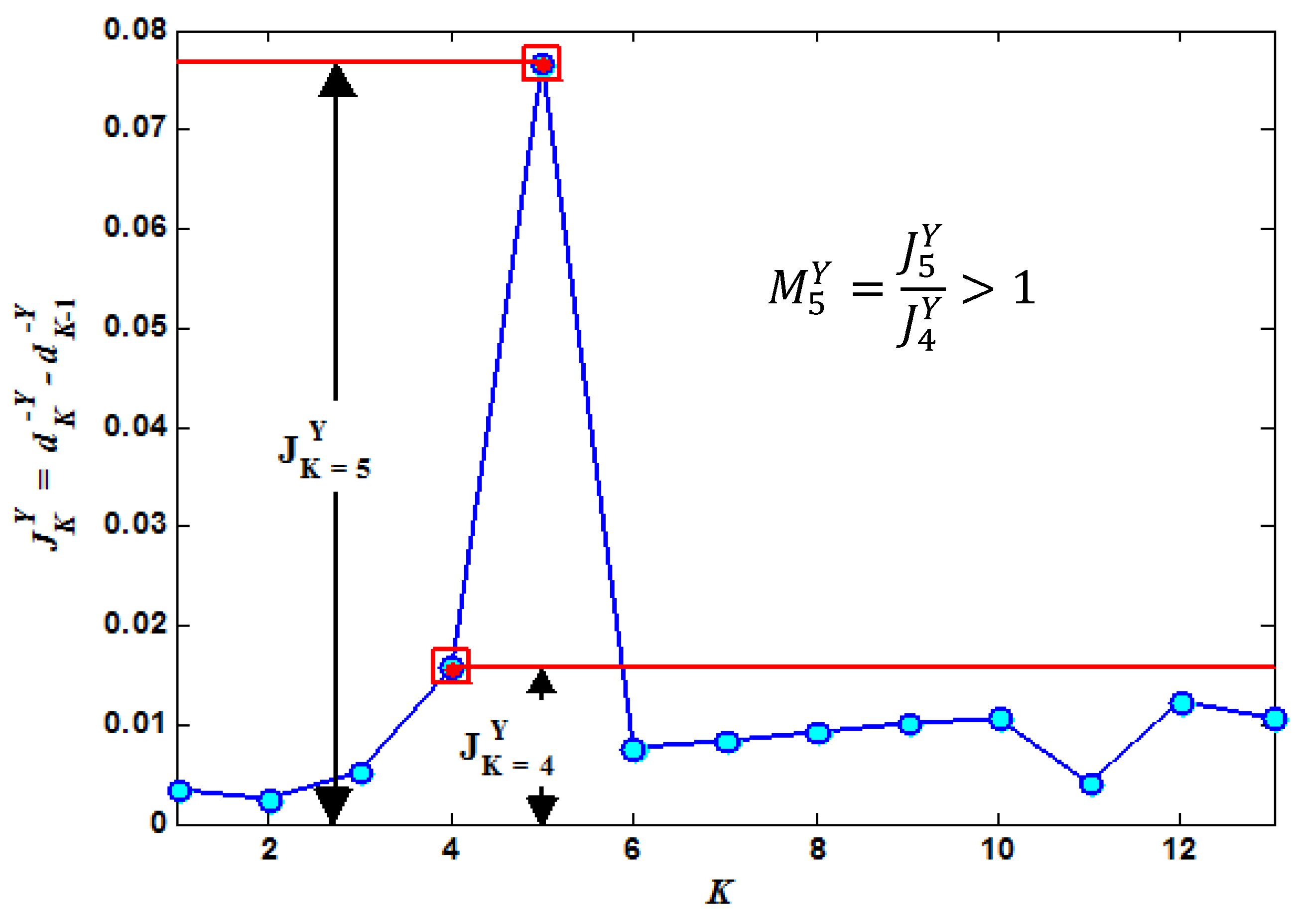
The larger the value of the margin operator becomes, the better (or more obvious) the cluster configuration, see Figure 1. Thus, by maximizing the margin value with respect to Y as in:

$$M_K^{*}={\text{max}}_{Y>0}\left\{ M_K^Y \right\}$$

(4)

the margin operator will quantify the quality of a clustering configuration with K partitions in terms of cluster compactness and the degree of de-correlation of its variables. Hence, the best Y can be automatically estimated.

In the improved jump method [17], non-linearity is addressed by a Spectral Clustering (SC) technique, based on kernel Principal Component Analysis (kPCA) that maps the input data to a new space where the points belonging to the same cluster are collinear if the tuning parameter, σ², of a Radial Basis Function (RBF) kernel is adequately selected. The SC algorithm is trained by sampled points and solves an eigenvalue problem. The eigenvectors, along with the extended kernel matrix, are used to expand the solution to the rest of the points [23]. After projecting all points onto a unit hyper-sphere, spherical k-means [24] can be used to construct the d^*_K curve. Using this estimated distortion curve one can calculate the corresponding M^*_K for each configuration tested (i.e., M^*_K=1 ... M^*_K=Kmax). The largest margin estimates the number of clusters, K* (see Figure 1), and the appropriate tuning parameter, σ², for the construction of the kernel matrix (i.e., model selection). The clustering is readily obtained from the parameters thus found.

Figure 1. An illustration of the selection of K* = 5 from the largest margin operator. The jump statistics are generated from five 3D Gaussian clusters, where Y = 2.5. Figure from Reference [17].

Figure 1. An illustration of the selection of K* = 5 from the largest margin operator. The jump statistics are generated from five 3D Gaussian clusters, where Y = 2.5. Figure from Reference [17].

Applying this information theoretic approach to image segmentation requires the use of feature vectors based on the local histogram of each pixel in an image. First, the color levels of a preprocessed image are quantized to only N_q levels using the criterion of minimum variance. Next, for training purposes, the color-quantized image is sampled within windows centered at each sample pixel, and a normalized histogram is computed for each window. These histograms become the feature vectors for further analysis and encode information about local texture as well as color. A χ² score is then used to compare the pixels as computed from these histograms [25]. The χ² score is defined as:

$${\chi }_{ij}^2=\frac{1}{2}{\displaystyle \sum }_{k=1}^K\frac{{\left[h_i\left(b\right)-h_j\left(b\right)\right]}^2}{h_i\left(b\right)+h_j\left(b\right)}$$

(5)

where h_i and h_j are histograms for the windows located on the i^th and j^th pixels, and h_i(b) indicates the repetition frequency of the b^th bin (out of N_q bins) in the corresponding histogram for the i^th pixel. Finally, a χ²-RBF kernel and its kernel matrix can be computed from k(h_i,h_j) = exp(−χ²_ij/σ_χ²), where k(h_i, h_j) is the element in the i^th row and j^th column of the kernel matrix, and σ_χ is the kernel standard deviation, the tuning parameter which is varied systematically across a specified range of values during model selection. After the target cluster number, K*, and RBF tuning parameter, σ², are determined via model selection, an accurate image segmentation can be accomplished.

2.3. Edge Suppression and Adaptive Window Sampling

The histogram based χ² scores are computed for a sample of the image pixels due to the memory constraints of solving the subsequent eigenvalue problem. Sometimes it is advantageous to control the image sampling by rigorously excluding partial volumes. The Canny edge detector is a good choice for outlining edges with low error. A modified Canny edge detector that morphologically thins the edge outline to two pixels as the last step is used. Edge detection is done on all pseudo-color channels and their combinations. Furthermore, simple edge detection in the slice-direction is carried out by thresholding the RGB Euclidean distance between nearest neighbor voxel intensities in the slice (z)-direction, i.e., involving adjacent slices. Experiments with IJM segmentation of labeled normal brain data suggest that a threshold of 100 is optimal for segmentation of the BrainWeb data. The union of all of these edge outlines produces a wider edge mask; see, for example, Figure 3c. With this mask the partial volumes can be efficiently excluded from the sampling process.

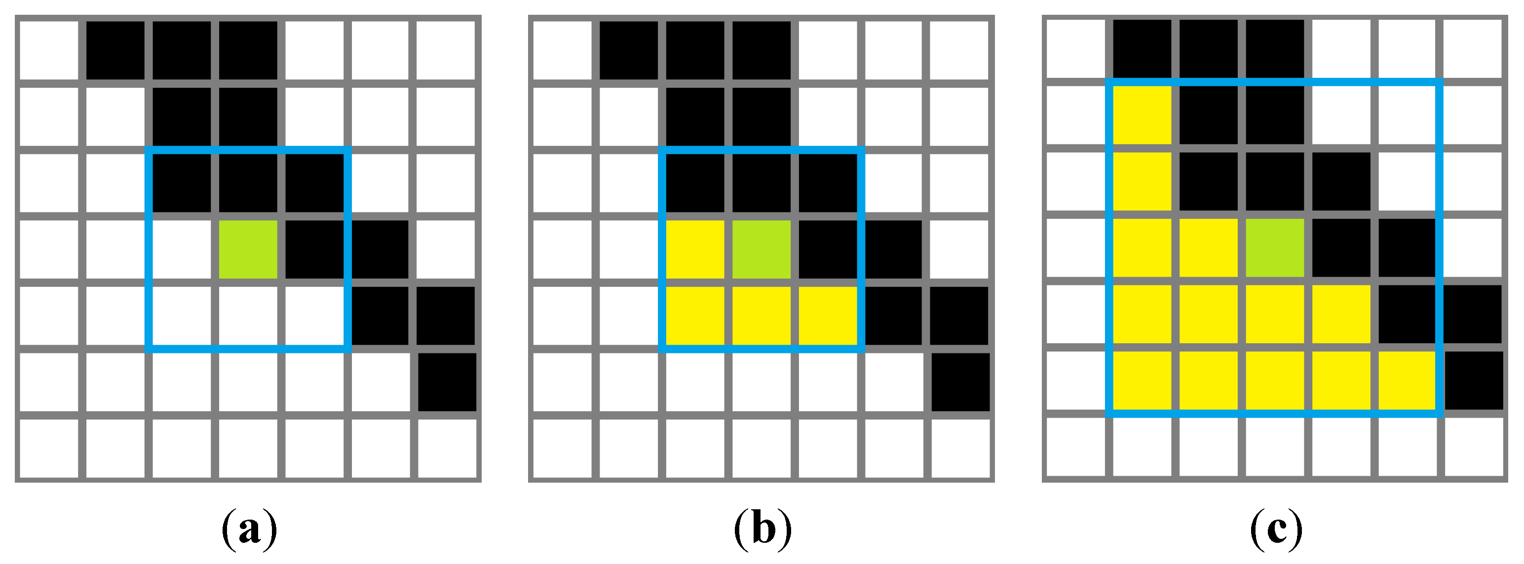
Adaptive windows are also used in concert with the edge suppression mask in the sampling and feature generation process for improved statistical representation. The sample windows are also dynamically enlarged when the local neighborhood is too small (we do this whenever it is smaller than the number of quantization levels, N_q), e.g., see Figure 2. Histograms of isolated points can be removed from the sampling process (we use a minimum requirement of N_q/2). Thus, a pixel near an edge can be more reliably clustered. For large bulky clusters with smooth boundaries this process is generally not necessary, but for difficult to separate segments (e.g., GM and CSF) edge suppression can yield much more stable and accurate segmentation results.

Figure 2. Adaptive window example with 3 × 3 window and N_q = 8 showing (a) the seed pixel (light green) and the initial window outlined in turquoise (b) The local neighborhood within the initial window has only 5 pixels, therefore (c) grow the local neighborhood until it has more than N_q pixels, restricted by the edge mask (black).

Figure 2. Adaptive window example with 3 × 3 window and N_q = 8 showing (a) the seed pixel (light green) and the initial window outlined in turquoise (b) The local neighborhood within the initial window has only 5 pixels, therefore (c) grow the local neighborhood until it has more than N_q pixels, restricted by the edge mask (black).

2.4. Post-Processing: Contrast Equalization and Enhancement via a Pseudo-Grayscale Conversion

This contrast equalization and enhancement are done by deriving an appropriate pseudo-grayscale conversion that is applied to each image. Consider the 3 RGB triples of the average values for normal tissues types 1, 2 and 3:

$$\begin{array}{c}a {\overline{R}}_1+b {\overline{G}}_1+c {\overline{B}}_1=I_{\text{b}}\\ a {\overline{R}}_2+b {\overline{G}}_2+c {\overline{B}}_2=I_{\text{b}}\\ a {\overline{R}}_3+b {\overline{G}}_3+c {\overline{B}}_3=I_{\text{b}}\end{array}$$

(6)

where $I_{\text{b}}\ne 0$ is the target background intensity, and the coefficients a, b and c can be automatically computed by Cramer’s rule. Now, the pseudo-grayscale conversion:

$$I_i=a R_i+b G_i+c B_i$$

(7)

for the i^th pixel will result in nearly complete suppression of distinctions between the three normal tissue types and effective separation of outliers, possibly an additional tissue type, as theoretically justified by Ref. [9]. The pseudo-greyscale transformation provides no control over the absolute contrast of any fourth tissue type, but its contrast is equalized against the other three, hence setting it distinctly apart and effectively segmenting it to a foreground. Note also that noise is reduced by a factor of $\sqrt{3}$. To enhance the contrast further, we determine the effective upper and lower intensity bounds for each slice. The low bound of the pseudo-grayscale image can be taken to be the predominant background intensity, the mode of which is I_b. The upper bound is taken to be the weighted maximum of all the grayscale image intensity maxima, V_max, selected based on a weighting with the brain ROI size for each slice, over the whole brain volume. This weighting ensures that outlier maxima in the smaller slices do not affect the overall contrast. This enhanced grayscale conversion is represented by:

$$I_i=\frac{255}{V_{max}-I_{\text{b}}}\left(a R_i+b G_i+c B_i-I_{\text{b}}\right)$$

(8)

Such transformation in Equation (8) allows us to construct global thresholds for all of the slices in the volume.

The segmentation of the full brain volume can now be automated, involving intensity-based and statistical techniques. Firstly, the maximum intensity for every slice is recorded and the global maximum is determined for the entire volume. The number of brain ROI voxels in each slice is also recorded. The global maximum intensity, V_max, for the grayscale images is thus found.

Secondly, the grayscale images are further contrast enhanced by Equation (8). The brain ROI is first morphologically filled and then eroded by diamond-shaped structural element, with six pixels between the central pixel and its edge, creating a brain boundary mask. Because the MS lesions are typically embedded in the WM they are usually not expected to be near the boundary of the brain ROI, but non-MS lesion outliers of the pseudo-grayscale transform can be there. One source of these other outliers is the proximity of non-brain tissues distorting the brain tissue intensity distributions [16]. Therefore, the brain boundary is always included with the background regardless of threshold.

The preliminarily segmentation of the foreground and background for each slice using the initial discrete threshold θ_d is carried out to hard cluster the grayscale pixels. Not every slice will have a foreground. An edge-suppressed mask, such as that applied to Figure 3c, is then applied to the foreground to develop a preliminary discrete mask. This discrete mask is then applied to the original pseudo-color image, and the pseudo-RGB average values are computed for the assumed MS lesions in that slice. Next, we update the segmentation of foreground and background for all slices using the slice-wise discrete threshold θ_d(s). The preliminary 0% fuzzy threshold, θ_0%(s), and the 100% fuzzy threshold, θ_100%(s) can then be determined via Otsu’s multi-threshold method [26] for each slice. Since MS lesions come in various sizes, they can be partially or fully saturated, thus, one would expect the histograms of the foreground to have three sub-clusters (fully saturated MS lesions, partially saturated MS lesions, partial volumes with surrounding tissues). The background will also have three sub-clusters due to non-MS lesion outliers near the boundary. Hence, Otsu’s method assuming two thresholds is applied on the foreground and background. The lower threshold is taken as θ_0%(s), of the slice, while the higher threshold is taken as θ_100%(s).

Figure 3. (a) The pseudo-color MR image encoding all major weightings for slice 105 of a BrainWeb brain volume with moderate MS lesions. Hyperintense MS lesions stand out as whitish spots; (b) the pseudo-color for slice 95 used to estimate tissue averages; (c) the 3D edge suppressed image of (a) that can be used as a sampling mask for further segmentation of non-WM tissues and again to estimate average tissue values.

Figure 3. (a) The pseudo-color MR image encoding all major weightings for slice 105 of a BrainWeb brain volume with moderate MS lesions. Hyperintense MS lesions stand out as whitish spots; (b) the pseudo-color for slice 95 used to estimate tissue averages; (c) the 3D edge suppressed image of (a) that can be used as a sampling mask for further segmentation of non-WM tissues and again to estimate average tissue values.

The overall discrete mask maximum intensity, D_max, and the standard deviation of the discrete mask maximum intensities, σ_max, for all relevant slices are determined. The global discrete and 0% fuzzy thresholds will then simply be taken as the median values of the thresholds for only the slices with maximum intensities I_max(s) > D_max − σ_max. Due to partial volume effects, such a median value for the 100% fuzzy threshold would be greatly underestimated. Instead the global 100% fuzzy threshold is computed by the average θ_100% = [D_max + max(θ_100%)]/2. Finally, the foreground and background are re-segmented using the corrected universal discrete threshold, θ_d.

Lastly, even in brains with MS lesions, usually not every slice will contain a lesion. Therefore we need to validate the clustering with the test:

$$I_{\text{max}}\left(s\right)>{\theta }_d$$

(9)

If the slice passes the test, then save the foreground binary image mask as the MS lesion discrete label for that slice. These binary images are further enhanced by morphological operations, e.g., filling holes. The global fuzzy thresholds, θ_0% and θ_100%, are used to define fuzzy labels for validated slices in a piecewise fashion, as well as using θ_d as the effective 50% fuzzy threshold. For intensity values below θ_d, the fuzzy label of the i^th voxel is computed as:

$$127.5\frac{I_i-{\theta }_{0\text{\%}}}{{\theta }_d-{\theta }_{0\text{\%}}}$$

(10)

and for intensity values above θ_d, the fuzzy label of the i^th voxel is computed as:

$$127.5\frac{I_i-{\theta }_d}{{\theta }_{100\text{\%}}-{\theta }_d}$$

(11)

where the labels are rounded to the nearest 8-bit non-negative integer.

3. Results and Discussion

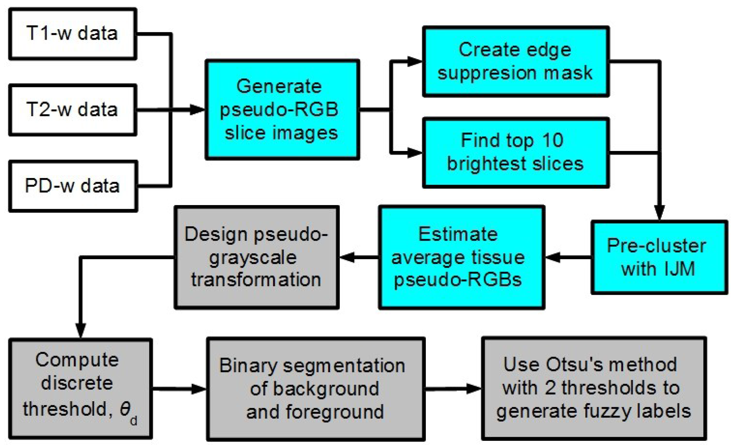
Pre-processed pseudo-color image of a slice derived from an MRI brain volume of a moderate case of MS lesion is shown in Figure 3. The MS lesions are strikingly brighter than the normal tissue types; this slice 95 is one of the overall brightest slices. This suggests that the grayscale image, derived from the proposed transformation of the pseudo-RGB image, ultimately might be adequate to segment the MS lesions from the rest of the brain. The grayscale transformation is built on top of the IJM pre-clustering, see the flowchart in Figure 4. It serves to simply segment any MS lesions from everything else.

Figure 4. Flowchart of the MS lesion segmentation process. Steps involving the pseudo-RGB images are highlighted in cyan. The subsequent steps using the transformed pseudo-grayscale image are highlighted in light gray.

Figure 4. Flowchart of the MS lesion segmentation process. Steps involving the pseudo-RGB images are highlighted in cyan. The subsequent steps using the transformed pseudo-grayscale image are highlighted in light gray.

3.1. Segmentation of MS Lesions in a Slice

3.1.1. Estimation of Pseudo-Color Tissue Intensity Averages via IJM Image Segmentation

IJM model selection consistently returns the most obvious clustering at K = 2 (WM separated from the rest of the brain) with RBF tuning parameter, σ² ≈ 5.5. The WM segment is identified as the segment as having the lower average grayscale intensity. Next, the non-WM segment is further segmented (K = 2 from IJM) into GM and CSF+ with σ² ≈ 0.2, where CSF+ denotes the CSF plus any other tissues. The GM segment is assumed to have the lower average grayscale intensity of the two resulting segments. Finally, the CSF+ segment is separated into CSF and MS lesions using a threshold of 185 in the “red” component, which is the average center of the gap in the “red” histograms of the CSF+ segment as shown in Reference [16]. It should be noted that no MS lesions are found in the normal brain at this point of the analysis.

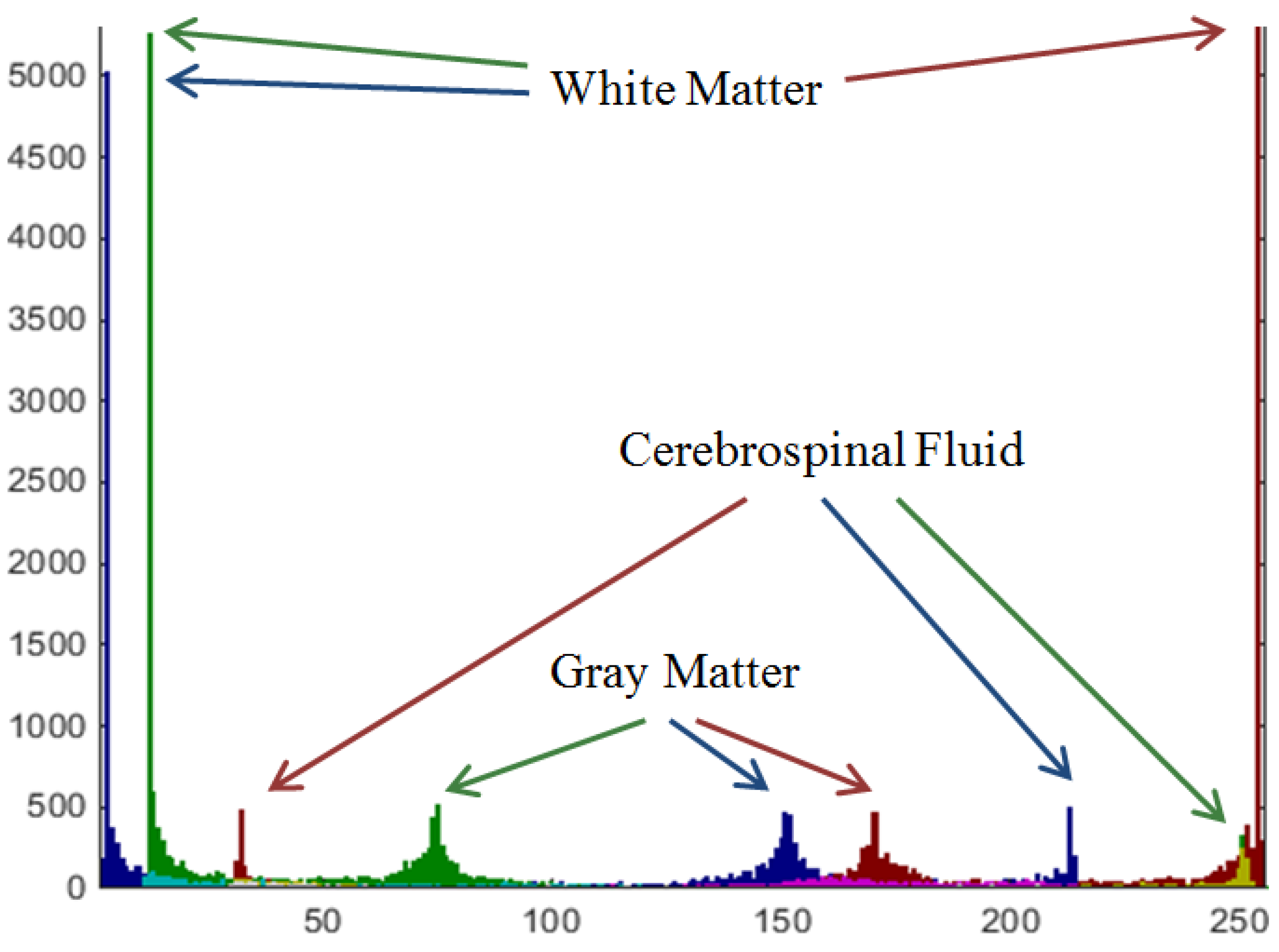
For the segmentation of normal brain MR images, a 3 × 3 window with number of quantization levels N_q = 8 is sufficient [1]. The segmentation results are made more stable by using a sample size of 5000 pixels in addition to the use of the edge suppression masked image of Figure 3c in the sampling process for the non-WM segmentation. For the moderate MS lesion brain, slices 82–90 and 95 are selected to estimate the normal tissue RGB values, and the segmentation of slice 95 via IJM is shown in Figure 5. The accuracy and reliability of this clustering are reported in Table 1, where the overall accuracy is 88.64%. The RGB histogram of slice 95 is shown in Figure 6. The average pseudo-RGB triples are estimated to be (253, 11, 2) for WM; (169.2, 74, 150) for GM; and (31, 250.1, 212.4) for CSF.

Figure 5. (a) Slice 95: IJM derived segmentation of the WM; (b) of the GM; (c) of the CSF; (d) of the MS lesions.

Figure 5. (a) Slice 95: IJM derived segmentation of the WM; (b) of the GM; (c) of the CSF; (d) of the MS lesions.

Table 1. Confusion matrix for slice 95 using IJM image segmentation in Reference [16] with edge mask.

Predicted/True	White Matter	Grey Matter	CSF	MS lesion	Reliability
Segment 1	8564	240	0	1	97.26%
Segment 2	676	5789	312	59	82.58%
Segment 3	1	616	1920	9	75.41%
Segment 4	21	1	0	98	81.86%
Accuracy	92.46%	87.11%	86.02%	58.68%	-

Table 1. Confusion matrix for slice 95 using IJM image segmentation in Reference [16] with edge mask.

Predicted/True	White Matter	Grey Matter	CSF	MS lesion	Reliability
Segment 1	8564	240	0	1	97.26%
Segment 2	676	5789	312	59	82.58%
Segment 3	1	616	1920	9	75.41%
Segment 4	21	1	0	98	81.86%
Accuracy	92.46%	87.11%	86.02%	58.68%	-

Figure 6. RGB histogram for slice 95 of moderate MS lesion data after the 12-bit to 8-bit pre-processing. The positions of the peaks for the main tissue types are indicated, and are consistent across the different slices due to pre-processing.

Figure 6. RGB histogram for slice 95 of moderate MS lesion data after the 12-bit to 8-bit pre-processing. The positions of the peaks for the main tissue types are indicated, and are consistent across the different slices due to pre-processing.

3.1.2. Contrast Equalization via a Pseudo-Grayscale Conversion

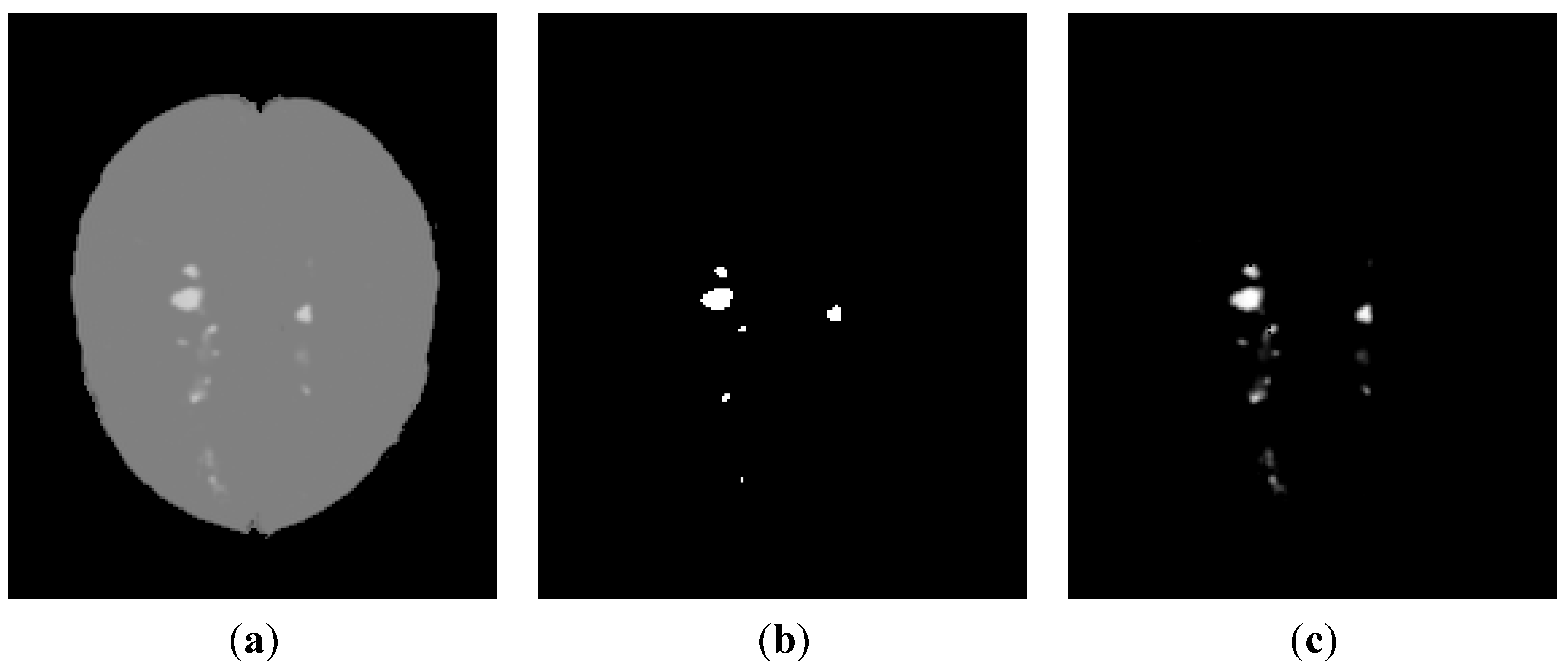
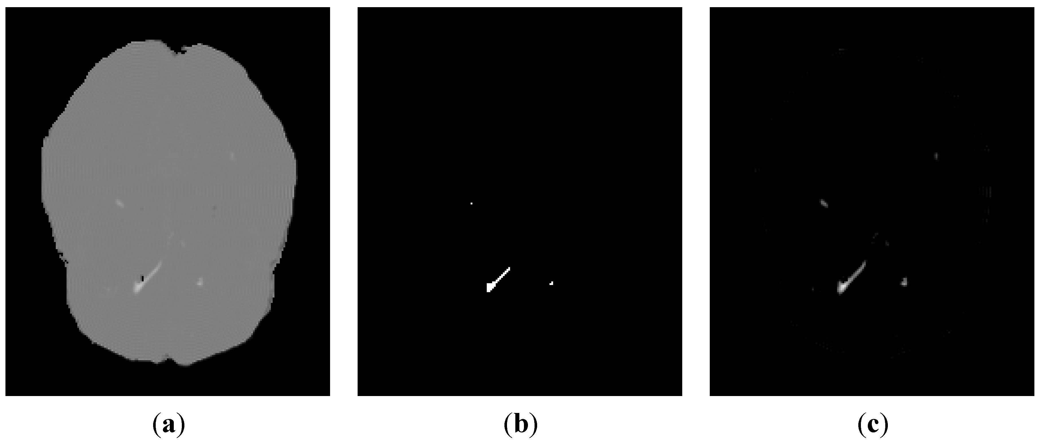
Setting the initial background to middle gray level value, I_b = 128, yields the pseudo-grayscale coefficients of Equation (6) as a = 0.4902, b = 0.3363, and c = 0.1351. Applying this pseudo-grayscale conversion to slice 105 in Figure 3a yields Figure 7a, which has background intensity mode of 128 and a maximum intensity of 207. Indeed, all three normal tissue types have very similar gray levels. Next, contrast enhancement takes the gray level values of 128 and 206 (the globally weighted maximum) as the bounds. Subsequent automated thresholding yields the global hard clustering threshold, θ_d = 110.14 for this volume. Both the discrete and fuzzy clusterings of this slice’s MS lesions are shown in Figure 7. The discrete ground truth for this slice is 112 MS lesion voxels, which are all found along with 12 WM voxels above the discrete threshold for this slice; yielding a sensitivity of 100%, while the reliability is 90.32%. The global 0% fuzzy bound is automatically determined to be 9.3176, where the background standard deviation, σ_b, for this slice is 12.5622. 100% fuzzy bound is found to be 237.4, and the foreground standard deviation is σ_f = 43.0250 for this slice. Fuzzy values are assigned in a piece-wise linear mapping between these two bounds and the discrete threshold. The 8-bit fuzzy ground truth total is 42817/255 ≈ 167.91, and the estimated fuzzy ground truth total is 42333/255 ≈ 166.01. Indeed, a visual inspection shows no visible difference and the image quality measures yield a mean-squared error (MSE) of only 1.9121, a signal-to-noise ratio (SNR) of 19.3297 dB, and a structural similarity (SSIM) index of 0.9965.

Figure 7. (a) Figure 3a after the initial pseudo-grayscale conversion by Equation (7) before contrast enhancement; (b) the result of the discrete clustering; (c) the result of 8-bit fuzzy clustering.

Figure 7. (a) Figure 3a after the initial pseudo-grayscale conversion by Equation (7) before contrast enhancement; (b) the result of the discrete clustering; (c) the result of 8-bit fuzzy clustering.

3.2. Segmentation of MS Lesions in a Whole Brain Volume

3.2.1. Brain Data with Mild MS Lesions

First, we examine the most challenging case of mild MS lesion brain data sets made available by BrainWeb. From IJM for the mild MS lesion data we find average modal pseudo-RGB triples as (251, 9.1, 9.3) for WM, (177, 48.4, 120.4) for GM, and (46, 241, 221.1) for CSF. These values are reasonable in spite of the small lesions. The pseudo-grayscale conversion is constructed by Equation (8) with coefficients: a = 0.4931, b = 0.2007, and c = 0.2575.

Applying this pseudo-grayscale conversion now to slice 69 yields Figure 8a, which has a background standard deviation, σ_b = 8.9134 and σ_f = 38.4408, comparable to the moderate MS lesion case. Subsequent automated thresholding yields a lower global discrete threshold of θ_d = 83.7481 and produces acceptable discrete and fuzzy labels for the MS lesions in this slice, seen in Figure 8. Only 41 voxels are above the discrete threshold, with ground truth labels of 19 MS lesions, 16 WM and 6 GM. The MS lesion total ground truth is 32 for this slice, so it only has a sensitivity of 59.38% and reliability of 46.34% for this slice. The method also struggles with the fuzzy segmentation as seen by the MSE = 12.2680, SNR = 4.9860 dB, and SSIM = 0.9877.

Table 2. Results for the binary discretely labeled MS lesion voxels (foreground) across the entire brain ROI of the mild, moderate and severe MS lesion brain data from BrainWeb.

	True Positive (TP)	True Negative (TN)	False Positive (FP)	False Negative (FN)	Ground Truth (GT = TP + FP)	Sensitivity TP/GT
mild	340	1954051	552	82	422	80.57%
moderate	3383	1951234	347	129	3512	96.33%
severe	9496	1941702	3375	608	10104	93.98%

Table 2. Results for the binary discretely labeled MS lesion voxels (foreground) across the entire brain ROI of the mild, moderate and severe MS lesion brain data from BrainWeb.

	True Positive (TP)	True Negative (TN)	False Positive (FP)	False Negative (FN)	Ground Truth (GT = TP + FP)	Sensitivity TP/GT
mild	340	1954051	552	82	422	80.57%
moderate	3383	1951234	347	129	3512	96.33%
severe	9496	1941702	3375	608	10104	93.98%

The whole brain discrete confusion matrix is summarized in Table 2, where the discretely labeled ground truth is 422 and the overall sensitivity is 80.57%. This case is pushing the limits of this method as the discrete threshold was automatically determined from only 13 qualifying slices and in the end MS lesions are found in only 67 out of 145 slices.

Figure 8. (a) Slice 69 of the MS lesion data after the initial pseudo-grayscale conversion by Equation (7) before contrast enhancement; (b) the binary discrete labels; (c) the fuzzy labels.

Figure 8. (a) Slice 69 of the MS lesion data after the initial pseudo-grayscale conversion by Equation (7) before contrast enhancement; (b) the binary discrete labels; (c) the fuzzy labels.

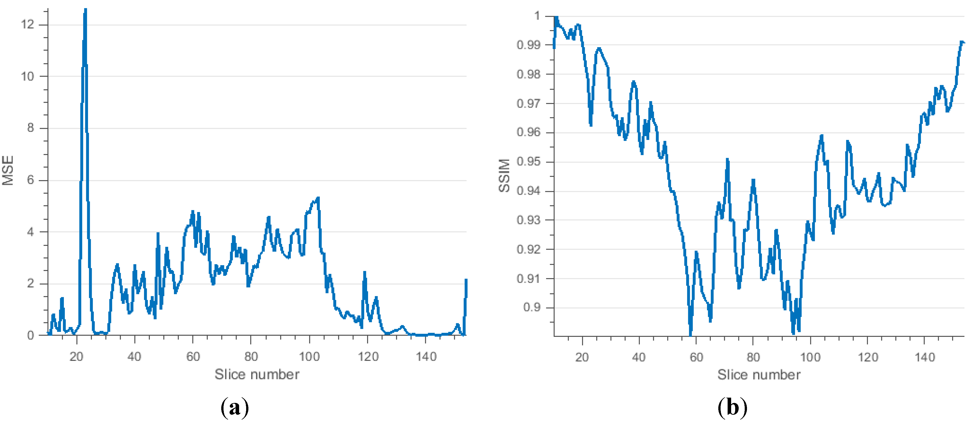
The estimated 8-bit fuzzy voxel total is 1305.5 compared to the fuzzy ground truth of 1162.4 voxels; see Table 3 for more comparisons. A comparison of performance slice-by-slice is shown in Figure 9. The estimated discrete and fuzzy labels follow the fuzzy ground truth quite well, with some overestimation with both labels. Finally, the MSE and SSIM of the fuzzy masks are shown in Figure 10.

Figure 9. MS lesion cluster counts from discrete (solid) and fuzzy (dashes) estimations compared to ground truths slice by slice in the brain ROI of the brain data with mild MS lesions.

Figure 9. MS lesion cluster counts from discrete (solid) and fuzzy (dashes) estimations compared to ground truths slice by slice in the brain ROI of the brain data with mild MS lesions.

Figure 10. (a) An MSE comparison of the estimated fuzzy label mask to the ground truth for mild MS lesion data. (b) An SSIM comparison of the same fuzzy masks.

Figure 10. (a) An MSE comparison of the estimated fuzzy label mask to the ground truth for mild MS lesion data. (b) An SSIM comparison of the same fuzzy masks.

Table 3. Comparisons measures for the discrete and fuzzy labels of MS lesion voxels across the entire brain ROI of the mild, moderate and severe MS lesion brain data, based on the results in Table 2.

	Specificity TN/(TN+FP)	Reliability TP/(TP+FP)	Dice Similarity Coefficient 2TP/(2TP+FP+FN)	Under Estimation FN/(TN+FN)	Over Estimation FP/(TN+FN)	Average Fuzzy SSIM
mild	99.97%	47.31%	0.5175	0.0042%	0.0282%	0.9029
moderate	99.96%	90.70%	0.8739	0.0066%	0.0434%	0.9468
severe	99.83%	73.78%	0.8266	0.0313%	0.1700%	0.9102

Table 3. Comparisons measures for the discrete and fuzzy labels of MS lesion voxels across the entire brain ROI of the mild, moderate and severe MS lesion brain data, based on the results in Table 2.

	Specificity TN/(TN+FP)	Reliability TP/(TP+FP)	Dice Similarity Coefficient 2TP/(2TP+FP+FN)	Under Estimation FN/(TN+FN)	Over Estimation FP/(TN+FN)	Average Fuzzy SSIM
mild	99.97%	47.31%	0.5175	0.0042%	0.0282%	0.9029
moderate	99.96%	90.70%	0.8739	0.0066%	0.0434%	0.9468
severe	99.83%	73.78%	0.8266	0.0313%	0.1700%	0.9102

3.2.2. Brain Data with Moderate MS Lesions

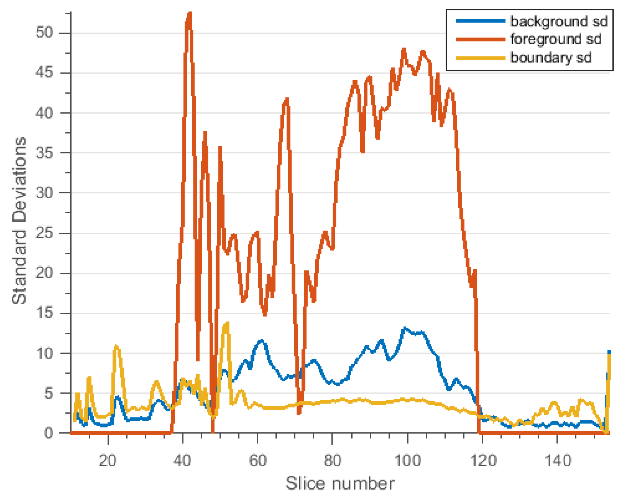
Next, we analyze the moderate MS lesion data. Applying this pseudo-grayscale conversion to all the slices containing the brain ROI (slices 10–154) yields a weighted global maximum intensity of 206. The variation of the foreground and background standard deviations by slice is shown in Figure 11.

Figure 11. Background, foreground and boundary standard deviations in slices 10–154 in the moderate MS lesion brain data from BrainWeb after pre-processing. Slices with no foreground detected are assigned 0 foreground standard deviation.

Figure 11. Background, foreground and boundary standard deviations in slices 10–154 in the moderate MS lesion brain data from BrainWeb after pre-processing. Slices with no foreground detected are assigned 0 foreground standard deviation.

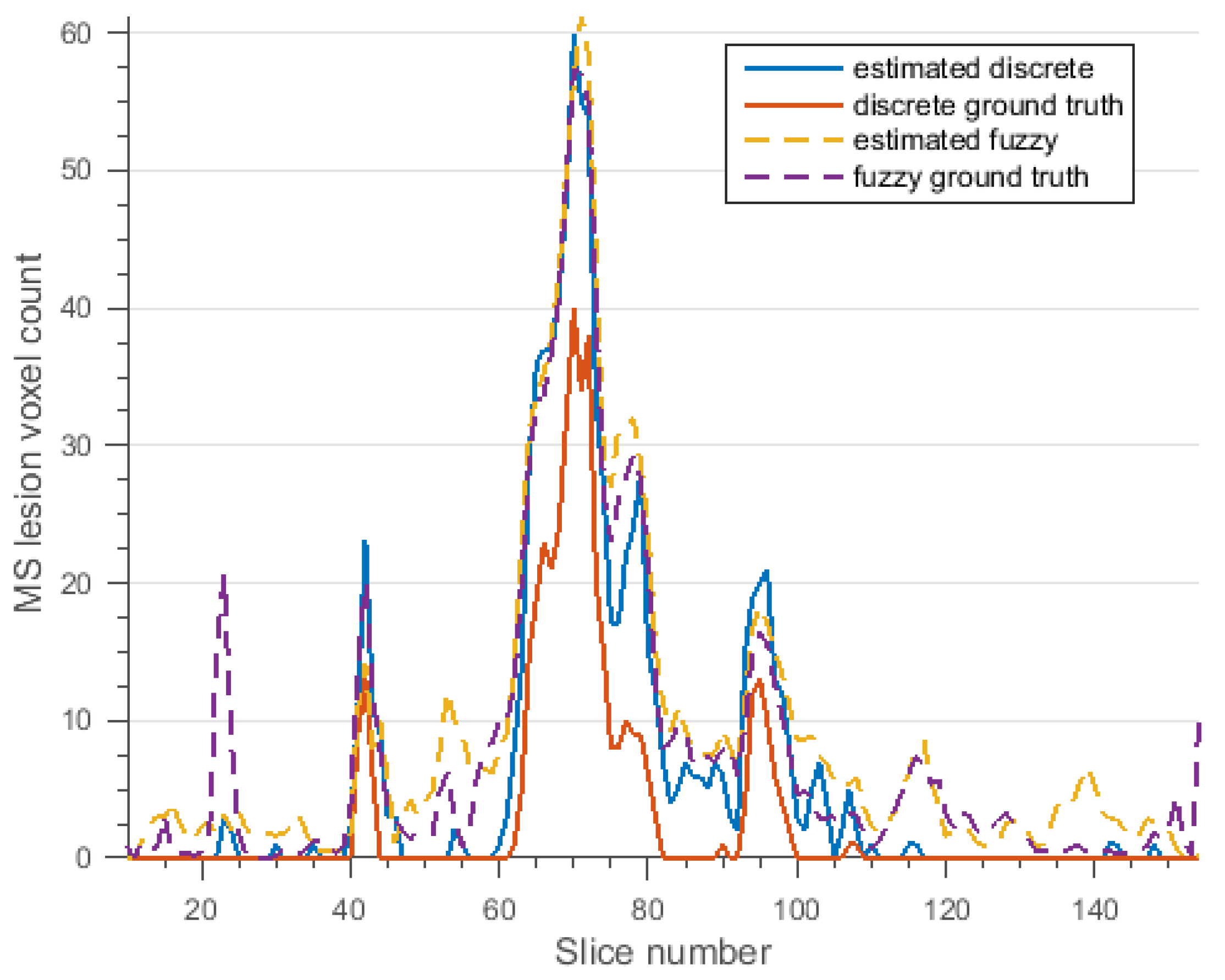
Our whole brain discrete segmentation results are shown in Table 2, where the discretely labeled ground truth is 3512 voxels. Our automated method estimates a fuzzy voxel total of 5903.8, compared to the fuzzy ground truth of 6697.5 voxels. A comparison of performance by slice is show in Figure 12, where the estimated discrete and fuzzy values almost always closely follow the ground truth values.

Figure 12. Moderate MS lesion cluster counts from discrete (solid) and fuzzy (dashed) estimates compared to ground truths, slice by slice, in the brain ROI.

Figure 12. Moderate MS lesion cluster counts from discrete (solid) and fuzzy (dashed) estimates compared to ground truths, slice by slice, in the brain ROI.

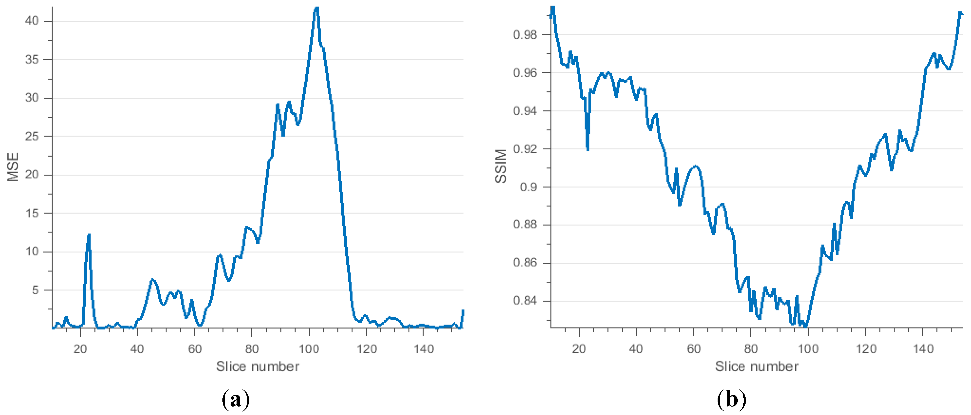
Various comparative measures for the discrete and fuzzy segmentation of the foreground and background are shown in Table 3. Note that the accuracy here does not include how well the WM, GM and CSF are segmented. Finally, the slice-by-slice MSE and SSIM between the fuzzy masks are shown in Figure 13.

Figure 13. (a) A comparison of MSE of the estimated fuzzy label mask to the ground truth for the moderate brain data. The spike at slice 23 is due to a segmentation failure of the fuzzy labels, see Figure 8. Figure 7 shows that this happens because these are anomalous MS lesions near the boundary of the brain. (b) An SSIM comparison of the estimated fuzzy label mask to the ground truth.

Figure 13. (a) A comparison of MSE of the estimated fuzzy label mask to the ground truth for the moderate brain data. The spike at slice 23 is due to a segmentation failure of the fuzzy labels, see Figure 8. Figure 7 shows that this happens because these are anomalous MS lesions near the boundary of the brain. (b) An SSIM comparison of the estimated fuzzy label mask to the ground truth.

3.2.3. Brain Data with Severe MS Lesions

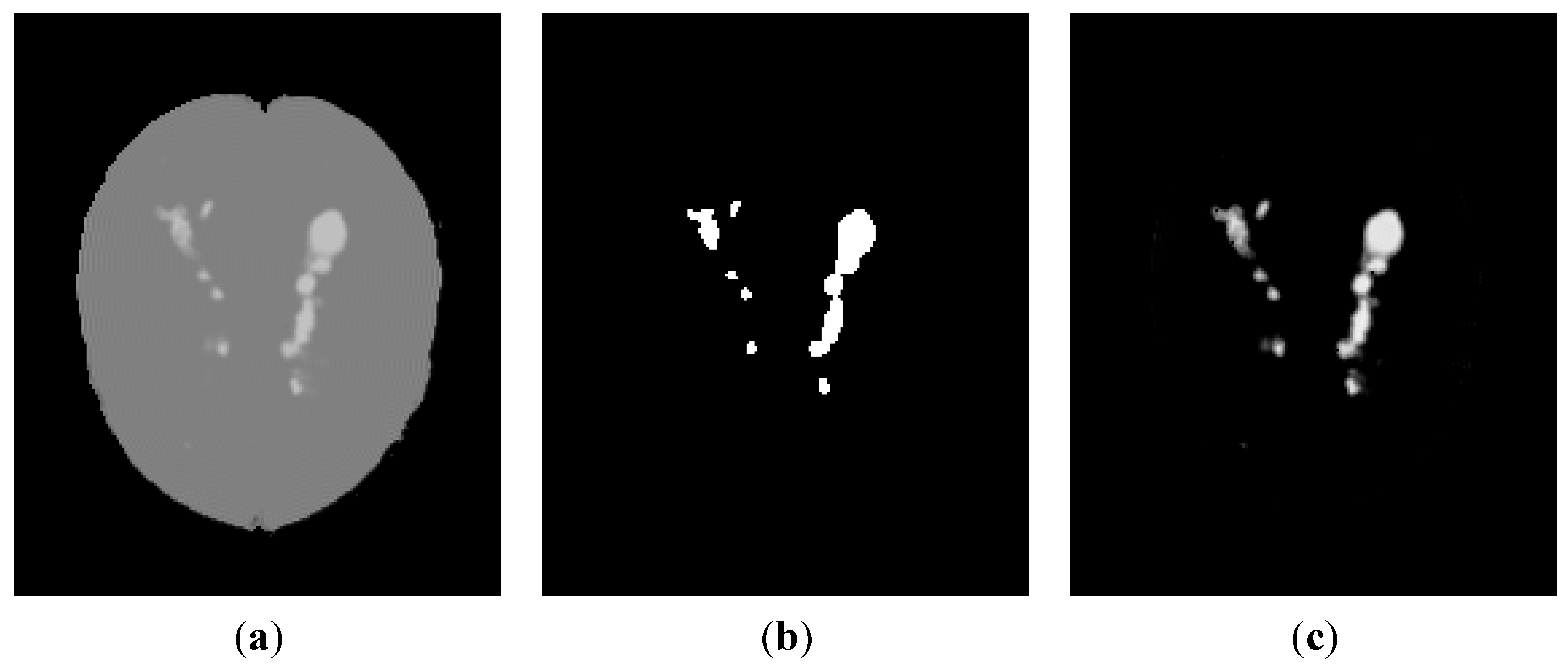
Finally, we apply our method of MS lesion segmentation to the severe MS lesion brain data sets made available by BrainWeb. The same steps were followed. For the severe MS lesion data we find average modal pseudo-RGB triples: (250.9, 8, 10) for WM; (176, 47.5, 120) for GM; and (46.8, 239.9, 218.9) for CSF. Similarly, the pseudo-grayscale conversion is constructed from coefficients: a = 0.4934, b = 0.1945 and c = 0.2661. These numbers are very similar to those found with the mild case. Applying this pseudo-grayscale conversion again to slice 105 yields Figure 14a, which has a background standard deviation, σ_b = 13.9411 and foreground standard deviation, σ_f = 47.2179, which are both slightly larger when compared to the moderate lesion case. The severe case has a larger variance because the estimated pseudo-RGB tissue averages are not as accurate as the moderate case due to the larger percentage of MS lesion voxels. Indeed, the presence of more lesions acts as an additive noise, causing the image histogram peaks to spread out. Subsequent automated thresholding finds θ_d = 97.9403 and still yields acceptable discrete and fuzzy labels for the MS lesions in this slice, as shown in Figure 14b,c, where the MSE = 36.5372, SNR = 12.4492 dB, and SSIM = 0.9838. The discrete ground truth for this slice is 523 MS lesion voxels, and our method finds 623, where 502 are actually ground truth labeled as MS lesion (95.98% sensitivity), 118 as WM, and 3 as GM (80.58% reliability). Our whole brain discrete segmentation results are shown in Table 2, where the discretely labeled ground truth is 10,104 voxels and the sensitivity is 93.98%. Our automated method estimates a fuzzy voxel total of 12,334, compared to the fuzzy ground truth of 12,855 voxels, see Table 3 for more details. A comparison of performance by slice is show in Figure 15, where we find that the estimated fuzzy labels almost always closely follow the fuzzy ground truth values. Finally, the MSE and SSIM of the fuzzy masks are shown in Figure 16.

Figure 14. (a) Slice 105 of the severe MS lesion data after the initial pseudo-grayscale conversion by Equation (7) before contrast enhancement; (b) the result of the discrete clustering; (c) the result of fuzzy clustering.

Figure 14. (a) Slice 105 of the severe MS lesion data after the initial pseudo-grayscale conversion by Equation (7) before contrast enhancement; (b) the result of the discrete clustering; (c) the result of fuzzy clustering.

Figure 15. MS lesion cluster counts from discrete (solid) and fuzzy (dashed) estimates compared to ground truths, slice by slice, in the ROI of the brain data with severe MS lesions.

Figure 15. MS lesion cluster counts from discrete (solid) and fuzzy (dashed) estimates compared to ground truths, slice by slice, in the ROI of the brain data with severe MS lesions.

Figure 16. (a) An MSE comparison of the estimated fuzzy label mask to the ground truth for severe MS lesion brain data. The profile follows Figure 9 due to consistent underestimation of the fuzzy labels. (b) An SSIM comparison of the same fuzzy label masks.

Figure 16. (a) An MSE comparison of the estimated fuzzy label mask to the ground truth for severe MS lesion brain data. The profile follows Figure 9 due to consistent underestimation of the fuzzy labels. (b) An SSIM comparison of the same fuzzy label masks.

4. Conclusions

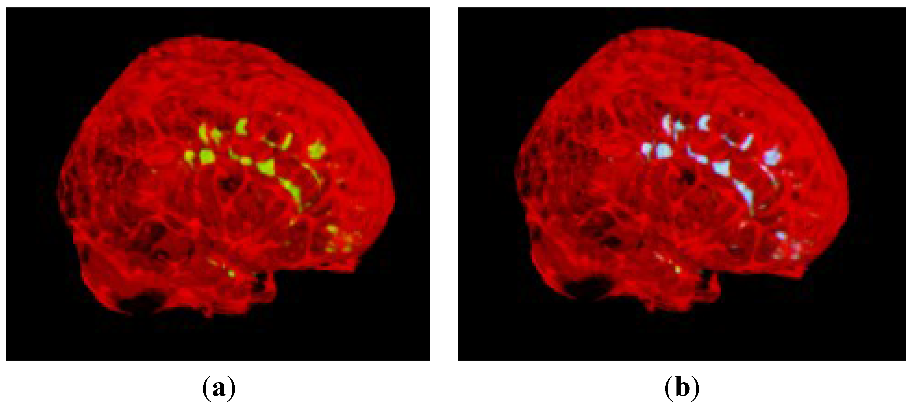
Three brains with MS lesions of different severities have been automatically segmented. We report a sensitivity (DSC) of 80% (0.5175) for the mild MS lesions, 96% (0.8739) for the moderate case, and 94% (0.8266) for the severe case; these are competitive with existing methods [15]. No MS lesions are found in the noiseless normal brain data from BrainWeb. The sensitivity of the severe case is reduced due to the larger volume of MS lesions slightly degrading the contrast equalization of normal tissues. The mild case has lower sensitivity due to the relatively small number of voxels that are fully within the lesion. Lesion voxels on or near an edge are, of course, suppressed by partial volume effects. Indeed, a Canny-based edge detector shows that only about 50% of the lesion voxels in the mild case are not on an edge, while the moderate and severe cases have over 70% of their lesion voxels inside the bulk. The discrete labels consistently perform well, and false positives/negatives are rather well balanced and limited to pixels neighboring the lesion. Furthermore, the algorithm gives a stable and reliable estimation of the MS lesion volumes for both discrete and fuzzy labels. The percentage differences of the overall fuzzy volumes are +12.31%, −11.85% and −4.05% for mild, moderate and severe, respectively. The robustness of the fuzzy labeling suggests the feasibility of this approach for clinical tracking of MS lesion volumes over the course of the disease [27]. The fuzzy labels can be also used to make a detailed three-dimensional visualization of the MS lesions; see Figure 17. Future work will deal with the effect of noise on the accuracy of detection of MS lesions of various severities as well as exploring the use of fluid-attenuated inversion recovery (FLAIR) and diffusion tensor imaging (DTI) MR data for detection of MS lesions.

Figure 17. 3D visualization of the moderate MS lesion brain: brain ROI indicated by a transparent ruby color, (a) only the fuzzy labeled ground truth (light green), (b) the estimated fuzzy labels (light blue) derived from our method superimposed over the ground truth (light green) from similar view points. Notice how small features are generally well captured. Used code is provided by [28].

Figure 17. 3D visualization of the moderate MS lesion brain: brain ROI indicated by a transparent ruby color, (a) only the fuzzy labeled ground truth (light green), (b) the estimated fuzzy labels (light blue) derived from our method superimposed over the ground truth (light green) from similar view points. Notice how small features are generally well captured. Used code is provided by [28].

The whole brain analysis is relatively computationally cost-effective when compared to tedious manual labeling. We executed our MATLAB code on a 64-bit Dell Optiplex 3020 with Intel Core i5-4570 CPU and 4 GB of RAM. Pre-processing of 12-bit data to 8-bit format takes only 15 s. Determination of the RBF tuning parameter, σ², takes about 4 min with 10 cross-validations (only required once). The segmentation and analysis of the “top ten” slices with IJM and a sample size of 5000 voxels takes about 3 min 20 s. The final step of intensity-based analysis of the complete brain executes in about 28 s. Therefore, repeated post-processing of the whole brain analysis can be handled in about 4 min with the current implementation. This time could be reduced with speed-ups, compiled executables and parallel computing.

References

1. Corona, E.; Hill, J.E.; Ao, J.; Nutter, B.; Mitra, S. An information theoretic approach to automated medical image segmentation. Proc. SPIE 2013, 8669. [Google Scholar] [CrossRef]
2. Miller, D.H.; Rudge, P.; Johnson, G.; Kendall, B.E.; Macmanus, D.G.; Moseley, I.F.; Barnes, D.; McDonald, W.I. Serial gadolinium enhanced magnetic resonance imaging in multiple sclerosis. Brain 1988, 111, 927–939. [Google Scholar] [CrossRef] [PubMed]
3. Horsfield, M.A. Magnetic Resonance Image Post-Processing for Multiple Sclerosis Research. Neuroimaging Clin. N. Am. 2008, 18, 637–649. [Google Scholar] [CrossRef] [PubMed]
4. Grimaud, J.; Lai, M.; Thorpe, J.; Adeleine, P.; Wang, L.; Barker, G.J.; Plummer, D.L.; Tofts, P.S.; McDonald, W.I.; Miller, D.H. Quantification of MRI lesion load in multiple sclerosis: A comparison of three computer-assisted techniques. Magn. Reson. Imag. 1996, 14, 495–505. [Google Scholar] [CrossRef]
5. Kikinis, R.; Shenton, M.E.; Gerig, G.; Martin, J.; Anderson, M.; Metcalf, D.; Guttmann, C.R.; McCarley, R.W.; Lorensen, W.; Cline, H.; et al. Routine quantitative analysis of brain and cerebrospinal fluid spaces with MR imaging. J. Magn. Reson. Imag. (JMRI) 1992, 2, 619–629. [Google Scholar] [CrossRef]
6. Bedell, B.J.; Narayana, P.A.; Wolinsky, J.S. A dual approach for minimizing false lesion classifications on magnetic resonance images. Magn. Reson. Med. 1997, 37, 94–102. [Google Scholar] [CrossRef] [PubMed]
7. Zijdenbos, A.; Forghani, R.; Evans, A. Automatic quantification of MS lesions in 3D MRI brain data sets: Validation of INSECT. Lect. Notes Comput. Sci. 1998, 1496, 439–448. [Google Scholar]
8. Sajja, B.R.; Datta, S.; He, R.J.; Meghana, M.; Gupta, R.K.; Wolinsky, J.S.; Narayana, P.A. Unified approach for multiple sclerosis lesion segmentation on brain MRI. Ann. Biomed. Eng. 2006, 442, 142–151. [Google Scholar] [CrossRef] [PubMed]
9. Van Leemput, K.; Maes, F.; Vandermeulen, D.; Colchester, A.; Suetens, P. Automated segmentation of multiple sclerosis lesions by model outlier detection. Medical Imag. 2001, 20, 677–688. [Google Scholar] [CrossRef] [PubMed]
10. Anbeek, P.; Vincken, K.L.; van Osch, M.J.; Bisschops, R.H.; van der Grond, J. Probabilistic segmentation of white lesions in MR imaging. Neuroimage 2004, 21, 1037–1044. [Google Scholar] [CrossRef] [PubMed]
11. Warfield, S.; Dengler, J.; Zaers, J.; Guttmann, C.R.G.; Wells, W.M., 3rd; Ettinger, G.J.; Hiller, J.; Kikinis, R. Automatic identification of gray matter structures from MRI to improve the segmentation of white matter lesions. J. Image Guid. Surg. 1995, 1, 326–338. [Google Scholar] [CrossRef]
12. Udupa, J.K.; Wei, L.; Samarasekera, S.; Miki, Y.; van Buchem, M.A.; Grossman, R.I. Multiple sclerosis lesion quantification using fuzzy-connectedness principles. IEEE Trans. Med. Imag. 1997, 16, 598–609. [Google Scholar] [CrossRef] [PubMed]
13. Admasu, F.; Al-Zubi, S.; Toennies, K.D.; Bodammer, N.; Hinrichs, H. Segmentation of multiple sclerosis lesions from MR brain images using the principles of fuzzy-connectedness and artificial neuron networks. In Proceedings of the 2003 International Conference on Image Processing, ICIP 2003, Barcelona, Spain, 14–17 September 2003; Volume 2, pp. 1081–1084.
14. Yoo, Y.J.; Brosch, T.; Traboulsee, A.; Li, D.K.B.; Tam, R. Deep Learning of Image Features from Unlabeled Data for Multiple Sclerosis Lesion Segmentation. In Proceedings of the 5th International Workshop, Machine Learning in Medical Imaging 2014 (MLMI14), Boston, MA, USA, 14 September 2014; Volume 8679, Lecture Notes in Computer Science. pp. 117–124.
15. Cabezas-Grebol, M. Altas-Based Segmentation of Multiple Sclerosis Lesions in Magnetic Resonance Imaging. Ph.D. Thesis, University of Girona, Girona, Spain, 16 July 2013. [Google Scholar]
16. Hill, J.E.; Nutter, B.; Mitra, S. An Information Theoretic Approach via IJM to Segmenting MR images with MS lesions. In Proceedings of the 2014 IEEE 27th International Symposium on Computer-Based Medical Systems (CBMS), New York, NY, USA, 27–29 May 2014; pp. 180–192.
17. Corona, E. Unsupervised Learning Methods: An Efficient Clustering Framework with Integrated Model Selection. Ph.D. Thesis, Texas Tech University, Lubbock, TX, USA, August 2012. [Google Scholar]
18. Corona, E.; Hill, J.E.; Ao, J.; Nutter, B.; Mitra, S. A novel unsupervised learning model for automated detection of precancerous abnormalities in uterine cervix with unified analysis of cervical cells and digital uterine cervix images. In Proceedings of the First IEEE Healthcare Technology Conference: Translational Engineering in Health & Medicine, Houston, TX, USA, 7–9 November 2012.
19. BrainWeb: Simulated Brain Database. Available online: http://brainweb.bic.mni.mcgill.ca/brainweb/ (accessed on 28 May 2015).
20. Lecoeur, J.; Wang, F.; Chen, L.M.; Li, R.; Aviso, M.; Dawant, B. Sub-millimeter Coregistration of Functional Maps across Imaging Sessions. In Proceedings of the 19th Annual Meeting of The International Society for Magnetic Resonance in Medicine (ISMRM), Montréal, QC, Canada, 7–13 May 2011.
21. Sugar, C.A.; James, G.M. Finding the number of clusters in a dataset: An information-theoretic approach. J. Am. Stat. Assoc. 2003, 98, 750–763. [Google Scholar] [CrossRef]
22. Hill, J.; Corona, E.; Ao, J.; Mitra, S.; Nutter, B. Information theoretic clustering for medical image segmentation. In Advanced Computational Approaches to Biomedical Engineering; Saha, P.K., Maulik, U., Basu, S., Eds.; Springer-Verlag: Berlin, Germany, 2014; pp. 47–70. [Google Scholar]
23. Alzate, C.; Suykens, J.A.K. Multiway spectral clustering with out-of-sample extensions through weighted kernel PCA. IEEE Trans. Pattern Anal. Mach. Intell. 2010, 32, 335–347. [Google Scholar] [CrossRef] [PubMed]
24. Dhillon, I.S.; Modha, D.M. Concept decompositions for large sparse text data using clustering. Mach. Learn. 2001, 42, 143–175. [Google Scholar] [CrossRef]
25. Fowlkes, C.; Belongie, S.; Chung, F.; Malik, J. Spectral grouping using the Nystrom method. IEEE Trans. Pattern Anal. Mach. Intell. 2004, 26, 214–225. [Google Scholar] [CrossRef] [PubMed]
26. Otsu, N. A Threshold Selection Method from Gray-Level Histograms. IEEE Trans. Syst. Man Cybern. 1979, 9, 62–66. [Google Scholar]
27. Elliott, C.; Arnold, D.L.; Collins, D.L. Temporally Consistent Probabilistic Detection of New Multiple Sclerosis Lesions in Brain MRI. IEEE Trans. Med. Imag. 2013, 32, 1490–1503. [Google Scholar] [CrossRef] [PubMed]
28. MathWorks. Available online: http://www.mathworks.com/matlabcentral/fileexchange/21993-viewer3d (accessed on 28 May 2015).