Article

Evaluating Solar and Wind Sustainability Across Countries Through National Development Levels and Resource Availability

1
Grupo de Energía Alternativa, Facultad de Ingeniería, Universidad de Antioquia, Calle 70 No. 52-21, Medellín 050010, Colombia
2
Energy Technology Group, Institute of Physics, University of Oldenburg, Carl-von-Ossietzky-Straße 9-11, D-26129 Oldenburg, Germany
3
Escuela Ambiental, Facultad de Ingeniería, Universidad de Antioquia, Calle 70 No. 52-21, Medellín 050010, Colombia
*
Author to whom correspondence should be addressed.
Technologies 2026, 14(9), 593; https://doi.org/10.3390/technologies14090593 (registering DOI)
Submission received: 11 August 2026 / Revised: 14 September 2026 / Accepted: 16 September 2026 / Published: 20 September 2026
(This article belongs to the Special Issue Emerging Renewable Energy Technologies and Smart Long-Term Planning)

Abstract

Life cycle assessment (LCA) is a crucial tool for monitoring the environmental impact of renewable energy systems. However, current approaches may not account for local socio-economic conditions and structural readiness without a large number of local data sets. The up-to-date carbon footprint assessment does not account for the huge gap between the maturity of infrastructure and the social context in different countries. To help bridge this gap, this work presents a new context-adjusted carbon-footprint assessment framework that embeds national preparedness and technological maturity into the LCA of solar photovoltaic (PV) and wind energy systems. The proposed model moves beyond traditional emission tracking by coupling site-specific resource availability, measured through the capacity factor (CF), with a technology development index (TDI). This index is an important indicator of socio-economic status and connects local economic conditions and energy infrastructures’ readiness. By employing different development scenarios in context, this study demonstrates the direct influence of structural differences on sustainability. The new socio-technical LCA approach that takes socio-economic and resource-specific factors into account in the context of development can be regarded as a robust and scalable tool to assess energy transitions across global contexts to ensure that equitable and rigorously informed decisions are made.

1. Introduction

Global warming and the unsustainable exploitation of natural resources are one of the most significant challenges of the 21st century, where human activities are the predominant determinants of this event [1,2]. Emissions of greenhouse gases (GHGs), mainly carbon dioxide (CO2), have resulted in notable environmental consequences, such as increasing global temperatures, extreme weather, and loss of biodiversity [3,4]. The energy sector, being heavily reliant on the intensive extraction and consumption of fossil fuels for electricity generation and industrial processes, forms a crucial factor in creating carbon emissions. Energy resources can be divided in renewable and non-renewable. Renewable energy sources, including solar, wind, hydropower, geothermal, and biomass, are naturally replenished and less environmentally degrading than non-renewable sources [5,6,7]. However, non-renewable energy resources, such as coal, oil, and natural gas, which rely on the extraction of finite resources, release large amounts of CO2 and other pollutants when burned [8]. Non-renewable sources still dominate worldwide energy use, despite the environmental benefits that sustainable resource management can offer. Recent figures reveal that fossil fuels are roughly 82% of total world energy supply in comparison with renewable energy, which provides only approximately 18% [9]. The main difference between renewable and non-renewable sources can be attributed not only to whether these sources are already there for use or how much each one of them contribute to the global energy supply; these differences are also associated with their environmental costs [10,11]. As renewable energies have gained importance as less polluting and climate-warming than green alternatives, non-renewables still dominate global consumption and are considered the leading contributors to GHG emissions [12,13]. This polarity of current fossil fuel dependence and the need for transitioning to more sustainable alternatives raises critical questions regarding the true environmental advantages and long-term resource stewardship of specific types of energy sources.
Utility-scale solar photovoltaic (PV) and on-shore wind systems are the backbone of the global energy transition and need to be well-engineered to integrate and utilize resources and operate efficiently. As a matter of fact, for the energy transition to accelerate, numerous national laws and incentives have been developed globally to make renewables more attractive in different economic and geopolitical contexts. For instance, industrialized economies, like Germany, have created aggressive laws and policies to promote the Energiewende and Renewable Energy Sources Act and accelerate decarbonization and capacity expansion in wind and solar energy generation [14,15,16]. In contrast, developing countries have developed systems in which there are specific policy tools to promote clean energy integration; Colombia has adopted current laws (1715 and 2099) with tax deduction, VAT exemption, and ambitious targets for carbon neutrality by 2050 [17,18,19], while Ghana uses the Renewable Energy Act and decentralized systems with feed-in tariffs to expand modern energy access and diversify its generation portfolio [20,21].
Previous studies on the environmental impact of renewable energy systems have been based on conventional LCA approaches, which usually employ global or regional average emission inventories. Even though the LCA method is effective in monitoring emissions across the cradle to the grave, its primary limitation is that it is far from capturing regional differences in operational processes, local weather patterns, and infrastructural readiness without the data-intensive local inventories required. Recent studies have attempted to incorporate spatial variation with respect to resource availability; nonetheless, they are often unaware of how national socio-economic maturity, maintenance processes, and grid efficiency affect real operational performance [22,23,24]. In contrast, the aim of this work is to address this issue by providing a more realistic and context-dependent approach. By linking the existing site-specific capacity to a composite technology development index (TDI), this approach bridges the gap between global inventories and national operational realities, providing a macro-level analysis without requiring high-level data collection for national scale.
In resource flows and environmental impact modeling, the carbon footprint is one of the most commonly used criteria for the classification and comparison of the environmental impact of various energy sources [25]. The coefficient measures CO2-equivalent (CO2-eq) emissions per unit of energy produced (i.e., the amount of emissions generated by producing 1 unit of energy for the lifetime LCA of each technology) [26,27]. It is important to assess carbon footprints to accurately quantify the benefits and costs of each technology (renewable vs. non-renewable) and why energy choices are important to address climate change. The core problem addressed in this study is that standard LCA methodologies fail to account for regional particularities, as capturing these geographical and structural variations accurately typically requires extensive process and site-specific data [22,23]. Furthermore, utility-scale solar PV and on-shore wind systems were selected as the primary technological focuses of this study, since they constitute the most globally mature and widely deployed renewable electricity generation options, while exhibiting fundamentally distinct technical and site-dependent characteristics in terms of resource intermittency, capacity factors, and infrastructure requirements. To address this issue, instead of trying to assess socio-economic conditions in terms of micro-economic or societal factors (e.g., local employment, land-use conflicts, or project profitability), this study develops and implements a more simple and context-aware carbon footprint assessment model in solar PV and on-shore wind energy. The methodology addresses the data-scarcity problem by combining site-specific resource availability (i.e., the capacity factor -CF- derived from global solar and wind atlases) and a new TDI that relates local economic conditions and infrastructure maturity, in terms of maintenance levels, with operational maintenance emissions. The CF and TDI adjustments are applied to provide an accurate and context-adjusted assessment of solar PV and wind energy systems in three countries with different levels of development: Germany, Colombia, and Ghana.

2. Methods and Materials

2.1. Greenhouse Gas (GHG) Emissions

The approach taken in this study relies on estimating the carbon footprint of various renewable energy technologies using a streamlined LCA method. This approach was preferred to cover GHG emissions associated with all stages of the system, including energy extraction, material production, construction, operation, maintenance, and decommissioning of energy infrastructure. In contrast to other methods that consider only the operational stage, LCA allows us to identify structural differences between technologies and gives a more reasonable overall picture of the long-run climate impact of these technologies. Emission factors (EFs), described in grams of CO2 equivalent per kilowatt-hour (g CO2e/kWh), are used to compute the calculation.
Table 1 presents the relative contribution of each life cycle assessment stage to the carbon footprint, expressed as g CO2e/kWh, for two renewable energy generation technologies: solar PV utility and on-shore wind utility.
The baseline EFs summarized in Table 1, which come from specific case studies in the research literature, are representative of global or regional averages that may not be fully transferable to other geographic contexts or unique local conditions. However, the evaluation of the environmental impact due to the site-specific performance variations requires that these standard EF values be adjusted with two parameters, CF and TDI. In percentage form, CF represents the average use of the nominal, installed capacity over the year, factoring in differences in availability within technologies as per availability differences between solar and wind. TDI takes into account the country’s level of development based on structural differences among countries with respect to innovation capacity, infrastructure quality, and institutional preparedness for renewable energy deployment. Regarding the temporal scope, the calculations presented in this study refer to annualized representative operational performance normalized over a standard 25-to-30-year asset operating life, instead of a dynamic multi-decadal time series. Consequently, annual module degradation, inverter replacements, and periodic major maintenance cycles are accounted for implicitly as averaged annual equivalents within the baseline life cycle emission inventories. Furthermore, to minimize confounding effects between national development levels and equipment vintage, the analysis standardizes its technological assumptions around contemporary utility-scale commercial specifications (such as modern silicon PV modules and IEC-class wind turbines) across all three comparative country contexts.

2.2. Capacity Factor

CF is an indicator for evaluating the actual performance of a power generation facility. It is defined as the ratio between the energy produced during a given period and the maximum possible energy output if the plant had operated continuously at its full rated capacity. Mathematically, it is expressed by Equation (1) [34,35,36].
C F = E r e a l P n o m i n a l × T
where E r e a l is the energy generated, P n o m i n a l is the installed capacity, and T is the number of hours within the period considered. This value depends on the availability and variability of the energy resource, the technological efficiency, and the geographical location. It is important to emphasize that the CF evaluated in this study represents modeled technical yields derived from resource availability databases. Consequently, these simulated metrics reflect theoretical technical potential and do not fully capture real-world operational limitations, such as grid curtailment, localized transmission congestion, forced outages, unpredicted component failures, or dynamic maintenance constraints. In the case of solar and wind energy resources, CF is estimated based on the available energy resource instead of on actual electricity generation. It is under these conditions that the evaluation follows the characterization of the main resource (i.e., the average solar irradiance and the wind speeds distribution). From this data, the potentially generable energy is computationally modelled with representative conversion parameters (e.g., the efficiency of a PV module or the power curves of wind turbines). Such methodological approach can provide for the assessment of the projected performance and the energy potential in places where there is no built operational infrastructure yet. Additionally, it provides a reference framework for technology deployment and investment planning. Nevertheless, once a sufficient level of installed capacity and operational generation data become available, the actual CF should be determined based on the net electricity effectively produced. It will then give a more accurate indication of plant behavior, since it incorporates multiple technical and process-related considerations such as the resource’s variability, system’s performance, regular and irregular maintenance, availability of equipment, and constraints of the power system.

2.2.1. Solar C F

For the case of solar energy, at a given location, the daily real energy ( E R e a l d ) output of a PV system can be estimated using Equation (2) [37,38].
E R e a l d = P n o m i n a l × P S H × P R
where PSH represents the peak sun hours at the site (h/day), defined as the total daily solar irradiation equivalent to a constant irradiance of 1 kW/m2. PR is the performance ratio, which accounts for all system losses due to temperature effects, inverter efficiency, wiring, soiling, shading, and module mismatch. To determine CF, the actual daily energy generated is divided by the maximum possible energy the plant could produce if it operated at nominal power for 24 h, as shown in Equation (3) [34].
C F = E R e a l d P n o m i n a l × 24
By substituting Equation (2) into Equation (3), Equation (4) is obtained.
C F = P n o m i n a l × P S H × P R P n o m i n a l × 24
Simplifying common terms yields, Equation (5) is obtained.
C F = P S H × P R 24
If PR is neglected in Equation (5), i.e., assuming ideal conditions with no losses due to temperature, inverter inefficiency, cabling, soiling, or mismatch, the expression for the solar CF can be further simplified. In this idealized case, CF depends solely on the ratio between PSH and the total number of hours in a day. Therefore, CF can be calculated using Equation (6).
C F = P S H 24
This ratio represents the fraction of the day during which the sun provides energy equivalent to its standard maximum irradiance (1 kW/m2). In other words, the PSH value corresponds to the number of hours per day during which the solar irradiance would need to remain constant at 1 kW/m2 to deliver the same total daily solar energy. Therefore, dividing PSH by 24 gives the proportion of time in a day that the PV system would operate at its rated power under ideal conditions. The processing methodology for the raw geospatial data, and the generation of final CF maps involves two primary data sources: global solar irradiance data in GeoTIFF format (.tif) and vector base maps for country outlines in shapefile format (.shp). The raw solar resource data were downloaded from the Global Solar Atlas with a high-resolution grid of approximately 10 m (or 9 arc-seconds). The computational work is carried out in two stages. In the first stage, the paths of the irradiance raster files and vector boundaries are defined. Each spatial data matrix is interpreted to denote the PSH and the CF is calculated on each file by Equation (6). To store the CF matrices in the database, the framework compiles and exports geospatial visualizations that either form a general regional map or a specific country outline plot for given visualization parameters. A very detailed geo-level analysis of solar CF values in Colombia, Germany, and Ghana is illustrated in Figure 1. Compiling the full solar irradiance information for each country, which it covers to the fullest extent, this map gives the power potential of PV nationwide. For example, the charts show high diversity of regions, since Colombia has high potential (CF > 0.20) along the Caribbean coastline but is more pronounced in La Guajira. In turn, Ghana has a strong north–south gradient with capacity conditions in the north (CF ≈ 0.16). Finally, Germany has a moderate CF gradient with the highest potential in the southern part (CF ≈ 0.14).
The national average CF values observed in these data suggest that Colombia has the highest total solar CF (0.14) and is mostly irradiated around the equator, while the second country (Ghana) has a CF of 0.12, and Germany has the lowest solar CF average (0.11), probably due to its high latitude and its frequent cloudy days. These national trends are also confirmed by city-level comparisons, with Medellín (CF = 0.14), being the highest CF value in Colombia and the most irradiated in the world year round. Oldenburg (CF = 0.099), located in Germany, is just below the national CF, showing how much different this is for different parts of Germany. In Ghana, Sunyani city is very similar to the country average (CF = 0.101) and thus generally reflects the reliable and moderate solar potential of the forest belt in Ghana.

2.2.2. Wind C F

The CF of a wind turbine or wind farm is the ratio between the actual energy generated over a given period and the energy that would be produced if the turbine operated at its rated power during all hours of that period. CF is the effective utilization of the wind resource at a site. High wind CF values suggest strong, steady winds and efficient turbine performance. The power available ( P d ) in the wind per unit area is given by Equation (7) [36,39].
P d = 1 2 ρ v 3
where ρ is the air density (kg/m3), and v is the instantaneous wind speed (m/s). Equation (7) describes the dependence of wind power on the cube of wind speed, meaning small variations in v lead to large differences in available power. The wind at a given site is not constant but varies over time according to a probability distribution. One of the most commonly used methods to describe it is the Weibull distribution, whose probability density function is expressed as Equation (8) [36,40,41].
f ( v ) = k c v c k 1 e v c k
where k is the shape parameter (dimensionless), and c is the scale parameter (m/s), representing a characteristic wind speed for the site. From this distribution, the mean v ¯ and cubic mean v ¯ 3 wind speeds can be obtained from Equation (9) and Equation (10), respectively [42,43].
v ¯ = 0 v f ( v ) d v = c Γ 1 + 1 k
v ¯ 3 = c 3 Γ 1 + 3 k
where Γ ( x ) is Euler’s Gamma function. The mean wind power density P d ¯ at a site is obtained by averaging the instantaneous power using the Weibull distribution and can be calculated using Equation (11).
P ¯ d = 1 2 ρ v ¯ 3 = 1 2 ρ c 3 Γ 1 + 3 k
It is important to note that a wind turbine converts only a fraction of the available power into electrical energy, which is determined by its aerodynamic power coefficient (Cp) and its overall mechanical and electrical efficiency ( η ). Cp represents the aerodynamic efficiency with which the rotor converts the kinetic energy of wind into mechanical power on the turbine shaft. The value of Cp is not constant, as it depends on the tip-speed ratio ( λ ) and the wind speed. Each wind turbine has a characteristic curve showing the variation of Cp with λ ; therefore, a maximum value is achieved under optimal operating conditions. In turn, η considers the losses due to mechanical transmission (e.g., gearbox, bearings, generator efficiency, power electronics (rectifier/inverter), and internal electrical losses). Therefore, the mean generated power for a wind turbine with a swept area A can be calculated as expressed in Equation (12).
P m e a n = η C P P ¯ d A
In this case, wind CF values based on the Weibull distribution can be obtained by dividing the mean generated power by the rated power of the wind turbine, as described in Equation (13).
C F = P m e a n P n o m i n a l = η C P 1 2 ρ c 3 Γ 1 + 3 k A P n o m i n a l
Equation (13) provides a realistic estimate of the CF based on the Weibull parameters and the technical characteristics of the wind turbine. If Weibull parameters are not available, the mean wind power can be expressed approximately in terms of the mean wind speed v ¯ . Therefore, Equation (14) can be used [36,44].
C F = P m e a n P n o m i n a l = η C P 1 2 ρ v ¯ 3 A P n o m i n a l
If the rated power is define as the power output at the rated wind speed ( v n o m ), P n o m i n a l can be calculated using Equation (15).
P n o m i n a l = η n o m C P n o m 1 2 ρ v n o m 3 A
where C P n o m is the power coefficient under nominal conditions; i.e., the value of Cp when the wind turbine operates at its v n o m and delivers its P n o m i n a l . η n o m indicates that this efficiency corresponds to the rated operating condition, when the turbine produces its nominal power. By substituting Equation (15) into Equation (14), Equation (16) is obtained.
C F = P m e a n P n o m i n a l = v ¯ v n o m 3 η η n o m C P C P n o m
Equation (16) allows us to estimate CF from the mean wind speed, the turbine’s rated wind speed, and the relative power and efficiency coefficient. For preliminary estimates of the CF, the ratios C P / C P n o m 1 and η / η n o m 1 were assumed. This approximation simplifies the analytical expression of CF, although it introduces potential bias when the site’s wind regime differs significantly from the turbine’s rated operating range, or when efficiency and control characteristics deviate from nominal behavior. The rated wind speed is chosen based on the IEC 61400-1 standard that is used for wind turbines. It is highlighted that the nominal wind speed of 10 m/s used in the evaluations is the usual wind speed of IEC Class II medium-sized commercial wind turbines utilized in the national regions studied. This decision is based on the design criteria, which is that the rated wind speed should be about 1.3 to 1.5 times the average wind speed of the target site; therefore, for a typical mean wind resource of 7 m/s, the rated wind speed is 10 to 11 m/s, so as to maintain the CF of the rotor system (Table 2).
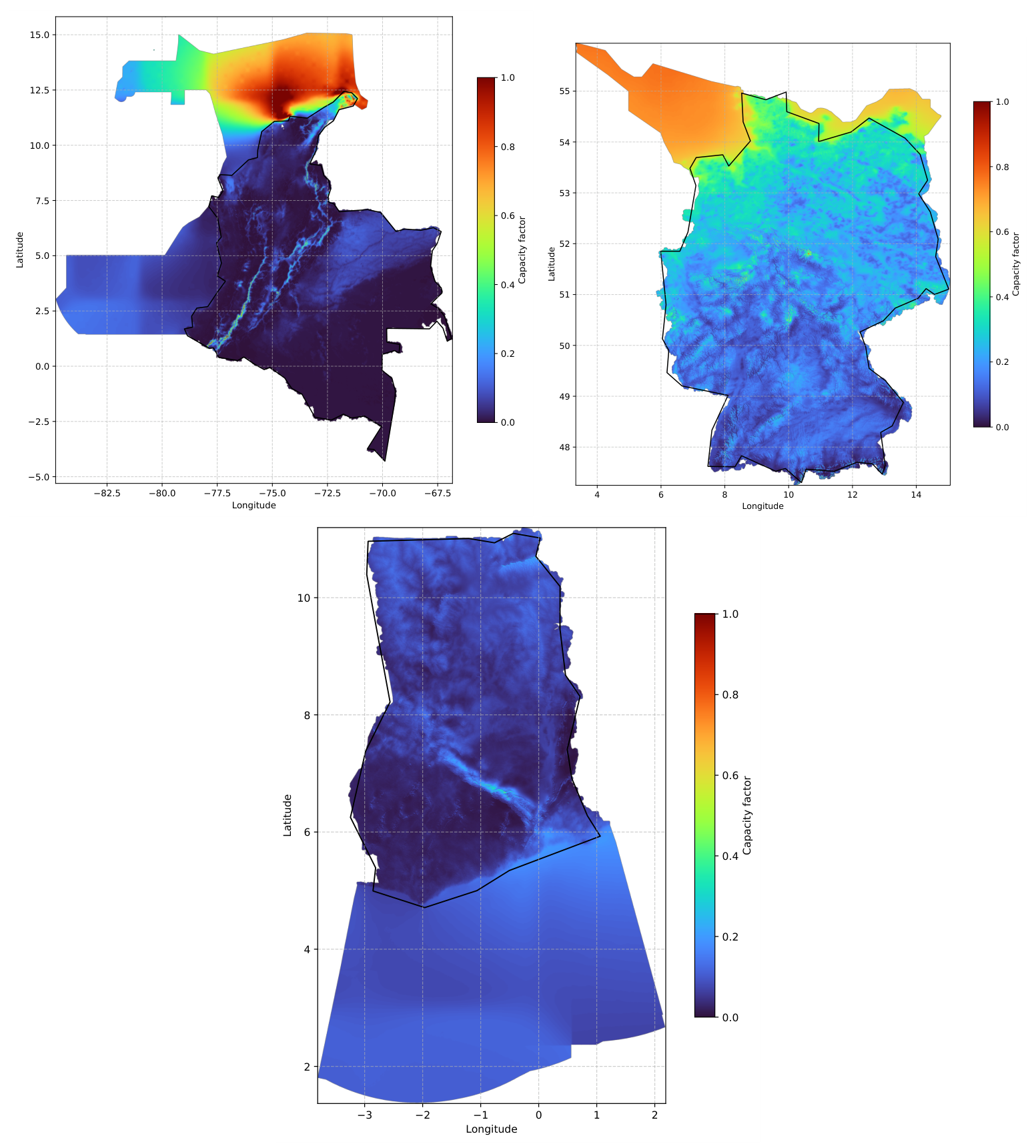
Figure 2 displays wind resource analysis results. This figure shows the local wind CF profile in Germany, Colombia, and Ghana. The wind power potential of each country is illustrated in the graph and shows the differences in the resource quality and geographic region. The maps also show CF values for on-shore and off-shore regions. It can be observed that the wind CF is significantly larger in off-shore regions, while it is similar for all three countries.
Wind CF maps were generated using a procedure analogous to the solar CF analysis, with the main differences lying in the input information and computation model. The average wind speed data was downloaded from the Global Wind Atlas platform with a spatial resolution of 100 m and was subsequently downscaled or processed to a standard height of 100 m. The vector base maps for Germany, Colombia, and Ghana, which were already prepared for the solar plots, were reused to mask the data. Finally, wind CF was computed based on Equation (16) to transform the wind speed data into the final CF values. The highest CF values are found in the northern coastal region in Colombia (i.e., in La Guajira), where wind speeds are consistently strong due to Caribbean trade winds. Colombia, however, has an average national CF of 0.16, which aligns with the contrast between very favorable northern zones and much lower CFs, such as Medellín, which has a CF of 0.044. These lowest inland values show limited prospects for large wind generation except in localized high-altitude corridors. In Germany, elevated CFs are present in the northern and coastal areas, as the country is primarily endowed with off-shore and North Sea wind resources. Germany has the highest CF average (0.27) of the three countries considered. City-level measurements validate such trends: Oldenburg, for instance, has a CF of 0.221, thus showing the high performance of northern locations. The CF gradually decreases in line with the southern interior, related to the lower average wind speed and rising land roughness. In Ghana, a relatively low CF is observed in most of the territory, creating a national average of 0.08, which is the lowest CF of the group. The southern coast exhibits slightly higher CFs, with maritime influences providing steadier winds, but values are still modest. The city of Sunyani, as an example, has a CF of 0.065, demonstrating the limited potential of wind energy in this area in relation to Colombia and Germany.

2.3. Technology Development Adjustments

In order to capture both the geographical impact and the country’s development level, a correction model was adopted that adjusts the CF values as a function of latitude and international reference values using the TDI. This index is used as a corrective factor for carbon footprint calculation to consider the structural differences among countries in terms of innovation ability, infrastructure quality, and institutional preparedness for renewable energy deployment. Since no single indicator can be comprehensive in capturing these dimensions, TDI is estimated based on the combination of aggregated indicators, such as those reported by the global innovation index (GII), the human development index (HDI), the renewable energy readiness index (RERI) as proposed by IRENA, and measures of reliability and quality of the electricity infrastructure reported by the World Bank and the IEA (INF). Although HDI is fundamentally a measure of broader human development rather than a direct metric of engineering maturity, it is incorporated into the TDI as a robust proxy for institutional capacity, workforce readiness, and general infrastructure reliability. In complex socio-technical systems, higher human development correlates strongly with the availability of skilled technical personnel, institutional efficiency in regulatory enforcement, and long-term maintenance capability, all of which directly mitigate operational downtimes and indirect maintenance emissions in renewable energy deployment. Each of these segments is scaled to 0–1, and then an integrated (i.e., a relative weight) index containing the main four components of technological innovation (w1 = 0.30), human development (w2 = 0.25), renewable energy readiness (w3 = 0.25), and electricity infrastructure (w4 = 0.20) was obtained. The general index formulation is given in Equation (17).
T D I = w 1 G I I + w 2 H D I + w 3 R E R I + w 4 I N F
where GII, HDI, RERI, and INF correspond to the normalized values of each indicator, and wi refers to the assigned weights. C F r e a l is the most determining variable. The adjustment was carried out using the relation shown in Equation (18).
C F r e a l = C F × ( 1 α ( 1 T D I ) )
where α was set equal to 0.25. This value was adopted as a sensitivity coefficient that weights the influence of TDI on the actual CF. The coefficient was derived from a literature review and empirical comparisons between renewable plants installed in countries with high infrastructure levels (TDI > 0.9) and those in developing countries (TDI < 0.4). Previous studies [49,50,51] report that losses associated with operational failures, limited spare part availability, grid constraints, and management deficiencies range between 15% and 25% reductions in effective energy conversion efficiency. Taking the upper bound of this range as a reference, α = 0.25 represents a scenario in which technological and socio-economic differences significantly affect plant availability, without overstating the effects in regions where systems already exhibit a certain degree of technological maturity. In this way, the adjustment is consistent with empirical performance data published by international agencies, which is accurate and ensures that the model does not overestimate the technological gap between developed and developing countries. It is acknowledged that these coefficients represent generalized macro-level scenario assumptions; thus, the framework is intentionally designed as a flexible, open architecture that can be refined with site-specific empirical coefficients as localized operational datasets become available.

2.4. Carbon Footprint

The carbon footprint of a system includes all GHG emissions generated throughout the different stages of the system’s life cycle, namely manufacturing, construction, operation, maintenance, and end of life (i.e., dismantling and disposal). In this study, the carbon footprint per unit of electricity generated (HC) was calculated as the sum of the contributions from each life cycle stage, as shown in Equation (19).
H C = E F m a n + E F c o n s + E o p + E F m + E F d p
Each term represents the emissions per unit of electricity generated, with units of g CO2e/kWh. In this equation, E F m a n refers to the emissions associated with the component manufacturing process; E F c o n s corresponds to the emissions from construction/installation activities (e.g., civil works, transportation, lifting, moorings, etc.); E F o p represents the operational emissions (i.e., direct emissions and auxiliary consumption); and E F m values are the maintenance-related emissions, which may also be adjusted according to the countries’ TDI, thus obtaining E F m R e a l (Equation (20)). E F d p accounts for the emissions associated with the decommissioning and end-of-life stage of the technology. The TDI may range from 0 (low-development countries) to 1 (high-development countries).
E F m R e a l = E F m × ( 1 + β ( 1 T D I ) )
The value of β = 0.2 was selected as a correction factor to reflect the relative increase in emissions associated with maintenance as a function of the technological development level of the country. In the maintenance phase, the information reported in the literature [49,50,51] indicates that differences are primarily manifested through higher fossil fuel consumption for spare part transportation, the use of less efficient auxiliary equipment, and more frequent maintenance schedules. These incremental impacts on emissions may be higher by around 10% up to 20% compared with reference values reported for highly industrialized countries. Hence, the upper value of the range, at β = 0.2 , was chosen as a conservative scenario that adequately captures the vulnerabilities of technologies deployed in less technically and logistically developed areas, without overestimating their influence on the overall life cycle outcome. This model distinguishes technologies according to application context, but it is consistent with life cycle analysis databases and the results of international organizations. Similarly to the macro-economic dimensions of this proof of concept, β is used as a bounding scenario parameter, leaving room for future adjustments tailored to specific regional supply chains.
The final adjustment of the carbon footprint to account for the geographical influence of the resource, as well as the influence of the country’s level of development, is based on the ratio between CF and C F r e a l .
H C r e a l = E F m a n + E F c o n s + E o p + E F m R e a l + E F d p C F C F r e a l
Through this formulation, Equation (21) dynamically scales the aggregated life cycle emissions according to the inverse ratio of regional CF, thereby capturing the direct trade-off between local resource availability and the environmental efficiency of the energy conversion process.

3. Results and Discussion

3.1. Case Study Scenarios

In order to test practical implementation of the proposed framework, a comparative case study was carried out examining the HCs of solar PV and wind energy technology in three separate geographical and economic settings, i.e., Germany, Colombia, and Ghana. These countries were selected to span an array of operational regimes, driven by their regional CF and differences in technical infrastructure at home. Germany has well-established renewable supply chains and extensive historical grid integration, with much of its industrial sector under lower average levels of solar irradiance [52,53], and sets a standard for significant technological and industrial development. Conversely, Colombia and Ghana represent scenarios with high, untapped renewable resource potential (contrasting CF profiles) and developing industrial supply chains in each technology sector. The diversification of Colombia’s historically hydro-centric matrix faces transmission bottlenecks in remote resource-rich areas, including La Guajira, and it is structurally dependent on imported technology [54]. On the other hand, Ghana’s transition paradigm still has poor performance under its Renewable Energy Master Plan due to limited grid infrastructure, high financing costs, and an overreliance on thermal backup measures, which inherently affect industrial technological efficiency and socio-economic distribution [55,56]. By scaling the life cycle EFs from Table 1 with the site-specific CF maps generated in the previous section, assessments can be rendered regarding the way in which the real-world environmental efficiency of renewable electricity generation is jointly determined by geographical, climatic, and industrial conditions.

3.2. Sensitivity Analysis of TDI, C F r e a l and Carbon Footprint Weighting

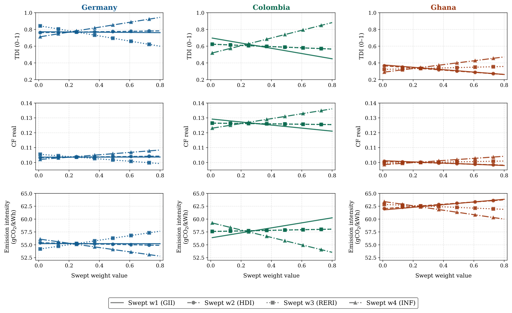
The final index can be then determined to understand potential biases by measuring the variation in baseline weights (w1 = 0.30, w2 = 0.25, w3 = 0.25, w4 = 0.20) for each of the four dimensions. The first of these sensitivity analyses changes the order of importance of GII, HDI, RERI, and INF indicators in order to quantify the role of these individual and combined indices on the TDI index. The sensitivity of TDI for parameter weight variation across Germany, Colombia, and Ghana is illustrated in Figure 3. The y-axis reflects the resultant TDI, C F r e a l and H C r e a l , and the x-axis denotes the weight being swept from the vicinity of 0.0 to 0.8 to provide an interpretative point of these plots. The different line styles correspond to the independent variation of a single parameter, the solid line representing the effect of w1 (GII), the dashed line with circles standing for w2 (HDI), the dotted line with squares representing w3 (RERI), and the dash-dot line with triangles referring to w4 (INF). After a sweep across the x-axis, the other three weights are adjusted to produce a total of 1.0.
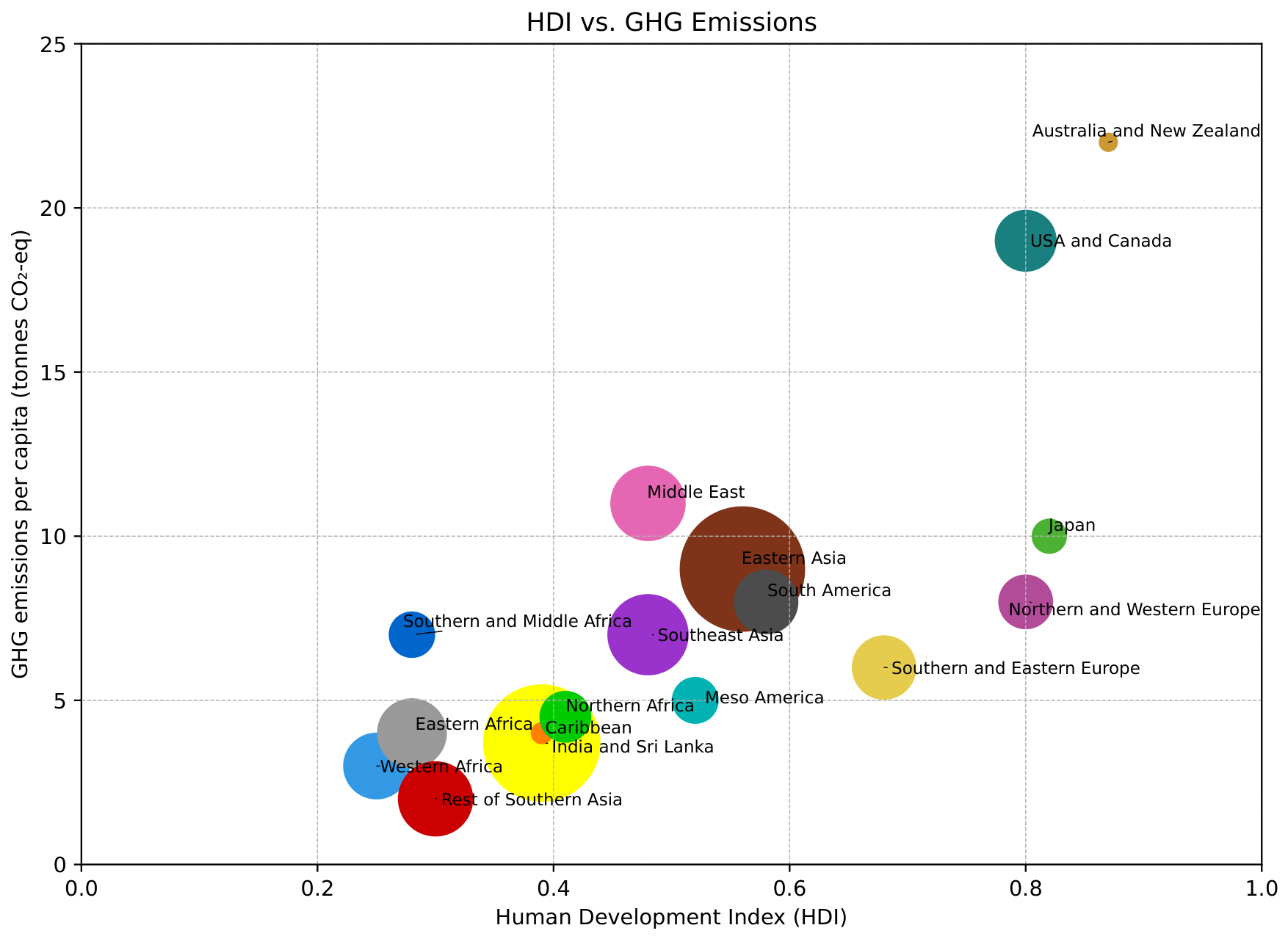
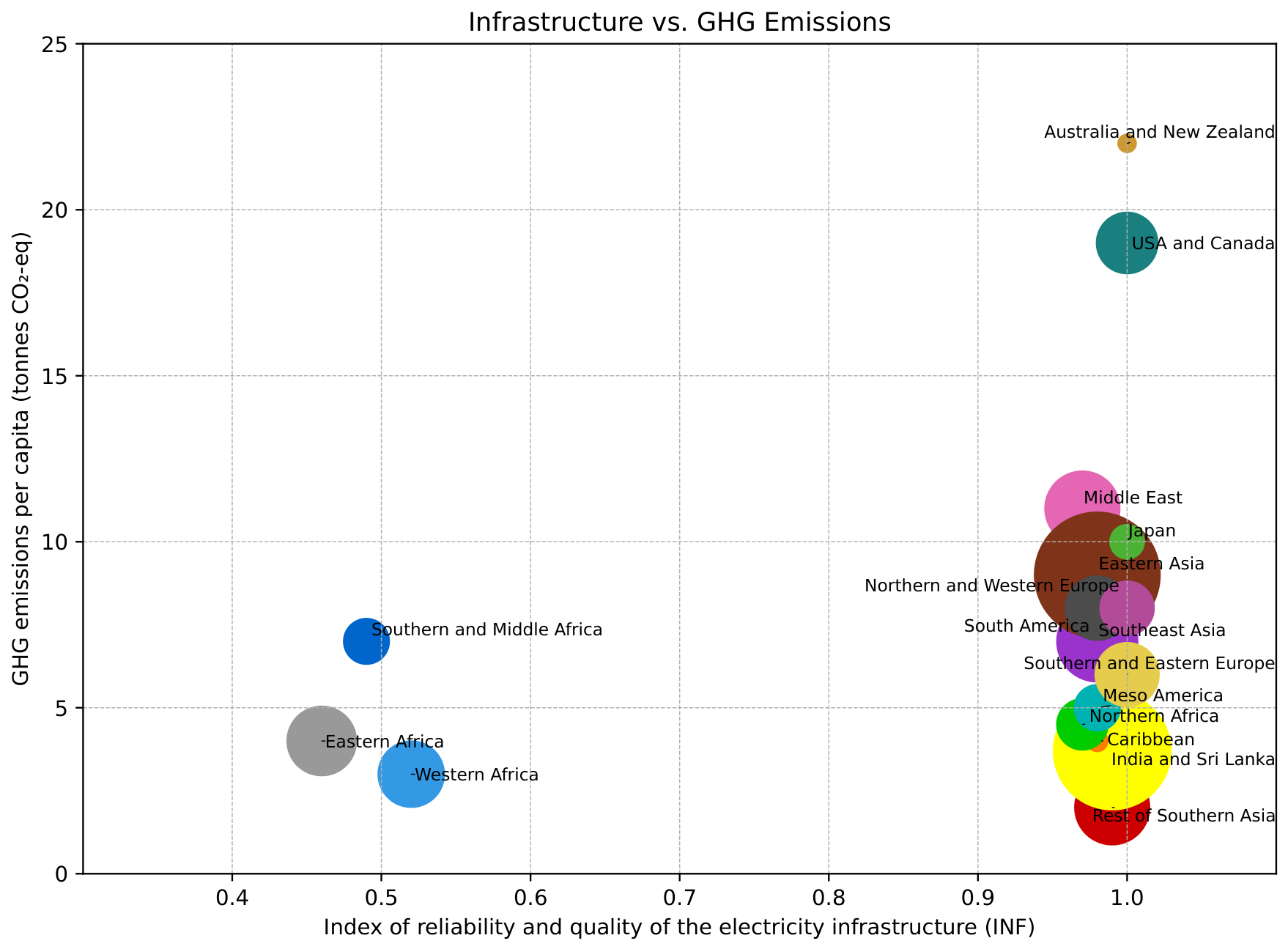
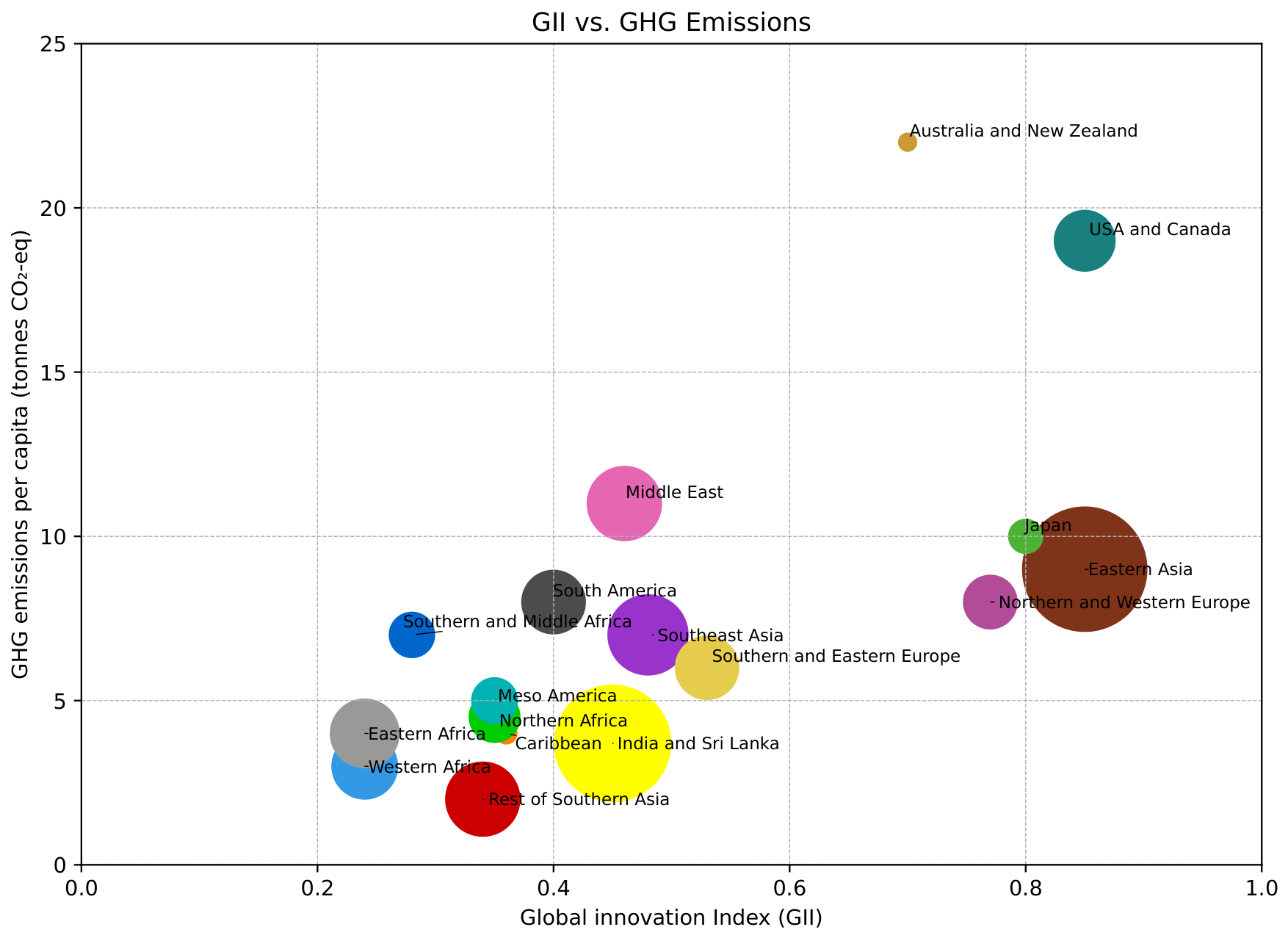
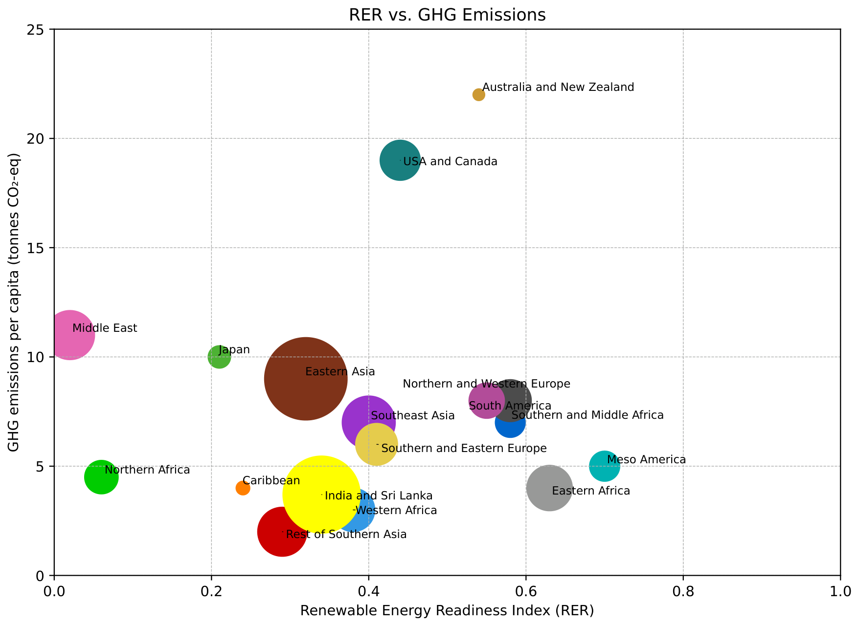
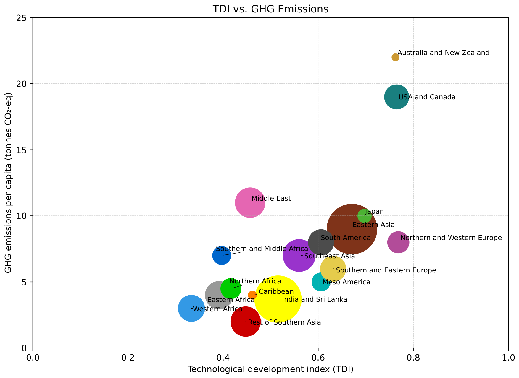
The structural nature of the TDI response is a function of the dispersion of the national baseline parameters for each country. For Germany, the estimated TDI runs the scale between around 0.61–0.94. This huge range is influenced by its extreme values associated with indicators: increased w4, which is the ideal INF (INF = 1.0), takes the score of the index over its maximum value (dash-dot line). By comparison, if its weakest parameter is overweighted (RERI = 0.55), then the TDI is pushed down to a figure close to 0.61 because of the sharply declining dotted line. Therefore, differences in the parameter w1 vs. w2 keep the index relatively constant at around 0.77, suggesting a balanced value. Meanwhile, Colombia has a much more dynamic response at its TDI level of approximately 0.59. It is calculated to have TDI over each of the weight sweeps varying from 0.46 to 0.89. The change with respect to w4, and its large INF (INF = 0.98), serves the largest role towards the final increment of the TDI score, in which the dash-dot line significantly goes up. However, increasing w1 (solid line) linearly decreases Colombian index. It demonstrates how some of the infrastructural strengths can lead to technology readiness assessment, given a significant degree of weight. Finally, Ghana is the most sensitive case and ranges around a low baseline TDI of about 0.36 and an interval of about 0.27 to 0.48. The large weight increases tend to depress the entire TDI as all the underlying indicators are less than 0.52. Since the RERI value is Ghana’s relatively the strongest parameter (RERI = 0.38), expanding the w3 weight (shown by the rising dotted line with squares) uniquely raises the computed TDI. Following the assessment of the TDI, the second row of Figure 3 illustrates the sensitivity of the real CF ( C F r e a l ) to the same parameter weight variations. In contrast to the highly variable index scores, C F r e a l demonstrates a much narrower band of sensitivity for three nations considered. Colombia exhibits the highest baseline C F r e a l at approximately 0.126, mathematically outperforming both Germany and Ghana, which hover near baselines of 0.104 and 0.101, respectively. For Colombia, sweeping the infrastructure weight w4 (dash-dot line with triangles) yields the most positive operational impact, raising C F r e a l toward 0.136, whereas an over-weighting of w1 (solid line) steadily reduces it to roughly 0.121. Germany and Ghana display relatively flat responses across most parameters, though increasing w4 provides a marginal improvement in both cases. Conversely, maximizing w3 in Germany and w1 in Ghana results in a slight depression of their respective CF values. This indicates that while the technological parameters strongly dictate the overall composite index, their influence on the actual operational CF is more subdued, even though it is strictly positive when the INF dimension is prioritized. Finally, the third row presents the sensitivity of the emission intensity, measured in g CO2/kWh, revealing distinct environmental profiles for each country. Ghana operates with the highest baseline emission intensity, at approximately 62.5 g CO2/kWh, followed by Colombia at 57.6 g CO2/kWh and Germany at 55.4 g CO2/kWh. There is a clear and consistent inverse relationship between the INF weight (w4) and the emission intensity. As w4 decreases toward 0.8, the emission intensity drops to around 60.0 g CO2/kWh for Ghana, 53.6 g CO2/kWh for Colombia, and 52.8 g CO2/kWh for Germany. On the other hand, if other baseline parameters are overweighted, there is a tendency to penalize the environmental performance. For Colombia and Ghana, increasing the weight of w1 (GII) drives the emission intensity to 60.2 g CO2/kWh and 63.8 g CO2/kWh, respectively. For Germany, the highest emissions are caused by the overweighting of w3 (RERI, represented by the dotted line with squares), which pushes the value to 57.6 g CO2/kWh. These responses from Germany, Colombia, and Ghana representing different levels of technology and infrastructure development further demonstrate the framework’s ability to assess complex national profiles with a base weighting approach. By extending this analytical analysis to a global scale, the scores can be used as a benchmark for macro-economic comparison. By measuring TDI, the countries can be classified as high maturity (0.75–1.0, e.g., Europe, North America or Japan), intermediate maturity (0.45–0.75, Latin America and emerging economies in Southeast Asia), and low maturity (<0.45, commonly found in Sub-Saharan Africa and some Central Asian countries). This operational evidence suggests that combining both the availability of resources at a site latitude with the technological capacity and the socio-economic capability of the individual countries results in a more differentiated and realistic calculation of the carbon footprint of different renewable technologies. Each index and the TDI-related overall results are presented in Figure 4, Figure 5, Figure 6, Figure 7 and Figure 8. Countries are illustrated by regions in these plots. The x-axis is the index of interest, while the y-axis is per capita CO2 emissions by region. The bubbles’ size also provides population by region, which can be statistically assessed for environmental impact and demographic weight.
In order to compare the environmental impact across the countries, the emissions are compared in terms of g CO2-eq/kWh, according to Equation (19). This information is then separated into the PV emission factors listed in Table 1 (manufacturing, construction, operation, maintenance, recycling, and decommissioning). The maintenance emissions are corrected with Equation (20) from the TDI on Figure 8 and the total life cycle emissions ( H C r e a l ), given by Equation (21). The CF value calculated in Equation (21) is the average CF of all three countries taken from the geographical maps described in Figure 1. It is important to highlight that while the final carbon footprint ( H C r e a l ) serves as the primary environmental metric, the analytical framework explicitly generates and evaluates critical intermediate contributions that dictate these final values. These include the high-resolution spatial CF derived from global resource databases, which quantify regional technical potential and the TDI scores (as well as their underlying infrastructural dimensions), which explicitly isolate national operational readiness and maintenance adjustments. Table 3 gives a comparative analysis of carbon footprint for solar PV technology in Germany, Colombia, and Ghana.
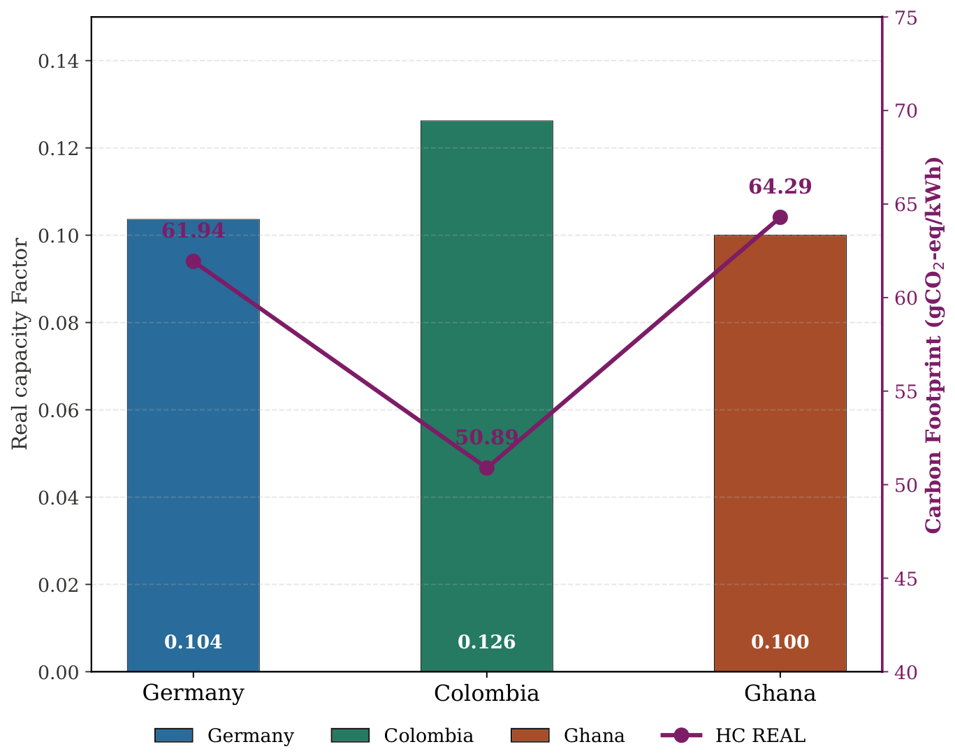
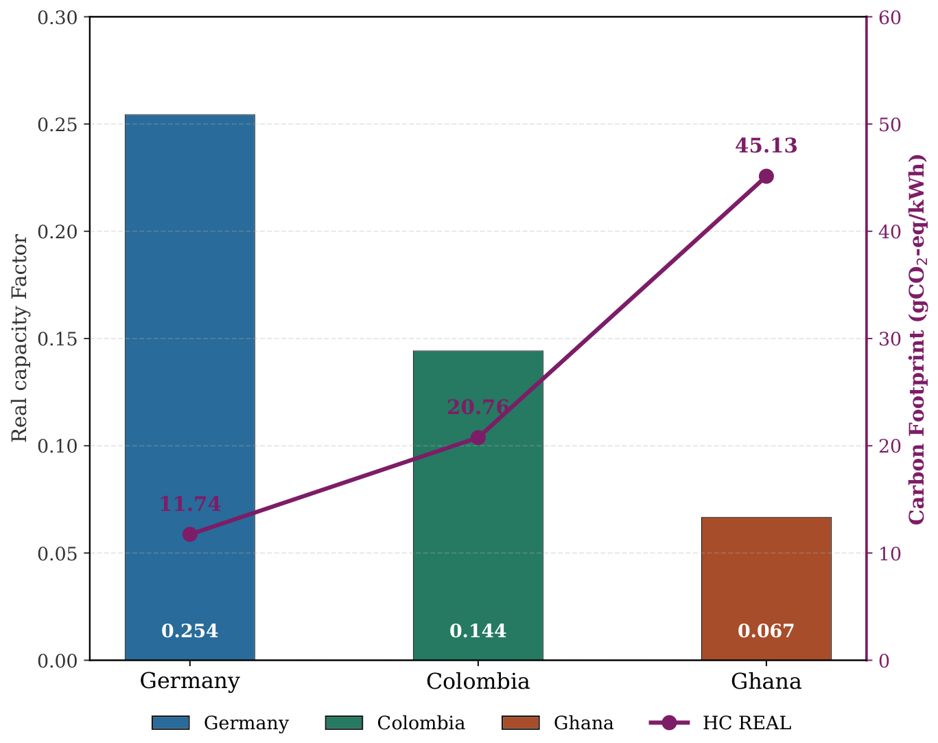
The comparison shows that although the unadjusted life cycle emissions (HC) baselines of the three countries are nearly the same (around 52.1 g CO2e/kWh), the impact of site-specific CF and technological maturity (TDI) on the final operational carbon footprint is significantly different. Colombia has the best emission intensity ( H C r e a l ) and is the most environmentally efficient country (50.89 g CO2e/kWh). Germany has a higher intensity (61.93 g CO2e/kWh), and Ghana is the most carbon-intensive country (64.29 g CO2e/kWh). These results show that the environmental benefits of solar PV deployment are not uniform and depend heavily on the regional climate and the performance of the equipment in each country. In this study, Colombia has the most abundant solar resources, having the highest CF (0.126). Such a high energy yield dilutes the embodied emissions of the PV systems over a larger volume of power generated. As a result, Colombia is able to maintain the lowest overall ( H C r e a l ) even with a low TDI (TDI of 0.606). With the resulting emission intensity per unit of energy being much higher for Germany and Ghana, a better geographical resource would be required in order to compensate for the environmental detriment of less mature local supply chains or a reliance on imported technologies. In contrast, with the technological infrastructure and the resource availability, Germany and Ghana are operating at different operational levels. Germany has the most technological maturity (TDI of 0.768) because of its optimized industrial processes and efficient maintenance and advanced end-of-life management. However, because of its low solar capacity factor (CF of 0.104), the total energy output is not sufficient enough to reduce the baseline lifecycle emissions as effectively Colombia does; therefore, the HC real value is high. A similar situation occurs in Ghana, which operates with the lowest CF (0.100) and TDI (0.333). Without the buffer of high energy yields or the mitigating effects of an advanced technological ecosystem to support efficient maintenance, Ghana’s PV deployment yields the highest specific emissions. The standardized regional comparison illustrates that the functional environmental impact of solar PV plants is driven by a complex balance between resource accessibility and technological life cycle management. While a high TDI is crucial for minimizing operational inefficiencies and reducing the carbon footprint of maintenance and manufacturing, a robust CF remains the dominant factor in driving down the per-kWh carbon debt. These findings underscore the necessity of evaluating both meteorological potential and local technological readiness when assessing the true climate mitigation value of renewable energy installations in diverse national contexts. On the other hand, the results from Table 4 and the corresponding visual analysis for on-shore wind demonstrate a significant shift in environmental performance compared to the solar PV scenario. Although the baseline emissions (HC) for wind are quite similar for all three countries (17.6 g CO2e/kWh), the actual emission ( H C r e a l ) can vary drastically based on the wind resource and technology maturity. Germany is the most efficient country and achieves a very low H C r e a l of 11.74 g CO2e/kWh (the most efficient country among the countries evaluated in this study). This is due to a strong synergy effect in which Germany is not only the most technologically mature country (TDI = 0.768) but also has a high wind CF (0.254). Colombia follows with its performance in the middle. The medium wind resource (CF = 0.144) and a slow technological maturity (TDI = 0.606) leads to an emission intensity of 20.76 g CO2e/kWh. The highest carbon footprint is found in Ghana at 45.13 g CO2e/kWh. The high emission intensity is coupled with a lack of wind resources (CF = 0.067) and insufficient technological infrastructure (TDI = 0.333). Without sufficient wind to generate high energy volumes, the fixed embodied impacts of the wind turbines cannot be efficiently diluted.
A cross-comparison of the two technologies reveals that on-shore wind systems exhibit substantially lower total life cycle emission intensities than solar PV systems across all three evaluated contexts. The baseline embodied carbon of wind turbine infrastructure (HC) is inherently lower per unit of generation potential than that of solar PV modules. This structural advantage is more apparent when there are moderate to high CF values. In Figure 9 and Figure 10, the two-axis charts (solar PV and on-shore wind) can be observed. The real CF (the bars on the top y-axis) is not much higher than the final carbon footprint (line on the bottom y-axis). For example, Germany reduced its carbon footprint from 61.94 g CO2e/kWh in the solar scenario to 11.74 g CO2e/kWh for wind, which is in stark contrast to the sharp increase in its wind CF (0.254) over solar CF (0.104). Colombia and Ghana also exhibit significant reductions compared to their PV profiles, dropping to 20.76 g CO2e/kWh and 45.13 g CO2e/kWh, respectively. The graphical representation highlights that while the solar H C r e a l trajectory remains relatively elevated and constrained, ranging only between 50.89 and 64.29 g CO2e/kWh due to universally lower baseline PV CF values, the wind scenario presents a much steeper dynamic range. The steep downward slope of the H C r e a l line in the wind chart visually underscores how systems with high mechanical energy yield can dilute their fixed embodied emissions.
The current analysis conducted relies on national-level aggregates and standardized life cycle inventories, which inherently smooth out regional micro-meteorological variations and localized supply chain carbon intensities. Hence, these national averages can be regarded as a proof of concept for macro-economic benchmarking based on micro-economic analysis rather than micro-site project evaluations. Furthermore, grid integration limitations, storage requirements, land use competition, and socio-economic or micro-economic aspects like project profitability, levelized cost of energy (LCOE), and local acceptance were not considered here. In addition, while a baseline end-of-life EF is used to close the life cycle inventory, institutional recycling procedures, long-term producer responsibility frameworks, and circularity of retired components were not considered in this study. Therefore, the results found in this research are based on the carbon footprint performance, instead of on the full circular economy principles.
In this regard, future research should focus on adding high-resolution spatial GIS data for the assessment of local resources, incorporating dynamic LCA frameworks to account for changing grid decarbonization trajectories, and expanding the comparative matrix to include hybrid configurations and advanced material alternatives, including bio-composites.
These results underscore that although the TDI is still important to minimize the carbon impact of manufacturing, maintenance and end-of-life processes, the operational CF dominates the carbon intensity. When a modern industrial base is combined with the best resource conditions (like Germany’s wind), then the emission intensity can be significantly minimized. Consequently, while on-shore wind is much less carbon intensive than solar PV, the right decarbonization strategy must be tailored to site-specific meteorological conditions rather than employing same technology.

4. Conclusions

The objective of this study was to develop and validate a context-dependent analytical framework that integrates site-specific CFs and a novel TDI to assess the life cycle carbon footprints of utility-scale solar PV and on-shore wind energy systems across distinct national contexts (Germany, Colombia, and Ghana). The main contribution of this research is to demonstrate that regional infrastructural maturity and local weather are important aspects in the improvement of environmental performance and that LCA inventories are actually quite wrong about the intensity of the emissions when local operations and industrial conditions are not considered. It was found that there are clear national differences regarding the TDI values. The average values of the base of TDI were 0.768 for Germany, 0.606 for Colombia and 0.333 for Ghana. All these values are equivalent to the infrastructural readiness, maintenance, and waste management of the system. When the CF values were also considered for each site, on-shore wind systems were found to be significantly less damaging in the life cycle than solar PV systems in all cases, since they dilute the emissions of fixed energy sources by higher mechanical energy. Specifically, high-resource operational environments combined with advanced industrial infrastructure, typified by Germany’s wind sector, minimize final carbon intensities down to 11.74 g CO2e/kW. Furthermore, the sensitivity analysis validated the mathematical robustness of TDI, revealing that highly developed infrastructural indices maintain stability against weighting fluctuations, whereas developing nations exhibit dynamic responsiveness tied to specific local technological constraints.
In this regard, renewable energy transitions need to be based on site-specific strategies where manufacturing efficiency, logistics, and regional industrial development are accounted with the raw resource potential. Furthermore, while less infrastructural development metrics may lead to operational or maintenance emission penalties, these findings should help identify the key entry points for specific interventions (e.g., grid planning, local capacity building, and maintenance supply chains). Therefore, policy recommendations at the country level should not be generalized to the national macro-economic average without project data.

Author Contributions

Conceptualization, L.V., A.P., T.B., A.G., H.T., E.C. and A.R.-C.; Methodology, L.V., A.P., T.B., A.G., H.T., E.C. and A.R.-C.; Software, L.V., A.P., T.B., H.T. and E.C.; Validation, L.V., T.B., A.G., H.T., E.C. and A.R.-C.; Formal analysis, L.V., T.B., A.G., H.T., E.C. and A.R.-C.; Investigation, L.V., A.P., T.B., A.G., H.T., E.C. and A.R.-C.; Data curation, L.V., A.P., T.B., A.G., H.T. and A.R.-C.; Writing—original draft, L.V., A.P., T.B., A.G., H.T., E.C. and A.R.-C.; Writing—review and editing, L.V. and H.T.; Visualization, L.V., A.P., T.B., H.T., E.C. and A.R.-C.; Supervision, L.V. and E.C. All authors have read and agreed to the published version of the manuscript.

Funding

This work is conducted as part of the DAAD-funded project Sustainable Energy Education—Developing Exchange between Continents (SEEDexchange, ID-57703987). The authors express their gratitude to the DAAD for the financial support provided for the development of this research. This project is the result of the collaboration between the University of Antioquia (Colombia), the University of Energy and Natural Resources (Ghana), the University of Oldenburg (Germany), and the non-governmental organization Change of World, whose joint efforts have contributed to strengthening research capacities and promoting international academic exchange in the field of sustainable energy.

Data Availability Statement

The original contributions presented in the study are included in the article, further inquiries can be directed to the corresponding author.

Conflicts of Interest

The authors declare that they have no conflicts of interest that could potentially influence the findings presented in this work.

References

  1. Mariappan, S.; David Raj, A.; Kumar, S.; Chatterjee, U. Global warming impacts on the environment in the last century. In Ecological Footprints of Climate Change: Adaptive Approaches and Sustainability; Springer: Berlin/Heidelberg, Germany, 2023; pp. 63–93. [Google Scholar]
  2. Bandh, S.A.; Shafi, S.; Peerzada, M.; Rehman, T.; Bashir, S.; Wani, S.A.; Dar, R. Multidimensional analysis of global climate change: A review. Environ. Sci. Pollut. Res. 2021, 28, 24872–24888. [Google Scholar] [CrossRef] [Scilit] [PubMed]
  3. Kabir, M.; Habiba, U.E.; Khan, W.; Shah, A.; Rahim, S.; De los Rios-Escalante, P.R.; Farooqi, Z.U.R.; Ali, L.; Shafiq, M. Climate change due to increasing concentration of carbon dioxide and its impacts on environment in 21st century; a mini review. J. King Saud Univ.-Sci. 2023, 35, 102693. [Google Scholar] [CrossRef] [Scilit]
  4. Shivanna, K.R. Climate change and its impact on biodiversity and human welfare. Proc. Indian Natl. Sci. Acad. 2022, 88, 160–171. [Google Scholar] [CrossRef] [Scilit]
  5. Rahman, A.; Farrok, O.; Haque, M.M. Environmental impact of renewable energy source based electrical power plants: Solar, wind, hydroelectric, biomass, geothermal, tidal, ocean, and osmotic. Renew. Sustain. Energy Rev. 2022, 161, 112279. [Google Scholar] [CrossRef] [Scilit]
  6. Makešová, M.; Valentová, M. The concept of multiple impacts of renewable energy sources: A critical review. Energies 2021, 14, 3183. [Google Scholar] [CrossRef] [Scilit]
  7. Hassan, Q.; Viktor, P.; Al-Musawi, T.J.; Ali, B.M.; Algburi, S.; Alzoubi, H.M.; Al-Jiboory, A.K.; Sameen, A.Z.; Salman, H.M.; Jaszczur, M. The renewable energy role in the global energy Transformations. Renew. Energy Focus 2024, 48, 100545. [Google Scholar] [CrossRef] [Scilit]
  8. Voumik, L.C.; Islam, M.A.; Ray, S.; Mohamed Yusop, N.Y.; Ridzuan, A.R. CO2 emissions from renewable and non-renewable electricity generation sources in the G7 countries: Static and dynamic panel assessment. Energies 2023, 16, 1044. [Google Scholar] [CrossRef] [Scilit]
  9. Energy Institute; Smil, V.; Ritchie, H.; Rosado, P. Statistical Review of World Energy (2025); Datos Procesados en *Energy Mix*. Basado en Smil (2017). Our World in Data. Available online: https://ourworldindata.org/energy-mix (accessed on 27 June 2025).
  10. Zohuri, B.; McDaniel, P.J. Introduction to Energy Essentials: Insight into Nuclear, Renewable, and Non-Renewable Energies; Academic Press: Cambridge, MA, USA, 2021. [Google Scholar]
  11. Algarni, S.; Tirth, V.; Alqahtani, T.; Alshehery, S.; Kshirsagar, P. Contribution of renewable energy sources to the environmental impacts and economic benefits for sustainable development. Sustain. Energy Technol. Assess. 2023, 56, 103098. [Google Scholar] [CrossRef] [Scilit]
  12. Apergis, N.; Kuziboev, B.; Abdullaev, I.; Rajabov, A. Investigating the association among CO2 emissions, renewable and non-renewable energy consumption in Uzbekistan: An ARDL approach. Environ. Sci. Pollut. Res. 2023, 30, 39666–39679. [Google Scholar] [CrossRef] [Scilit] [PubMed]
  13. Opeyemi, B.M. Path to sustainable energy consumption: The possibility of substituting renewable energy for non-renewable energy. Energy 2021, 228, 120519. [Google Scholar] [CrossRef] [Scilit]
  14. Plehwe, D.; Günaydin, K. Whither Energiewende? Strategies to manufacture uncertainty and unknowing to redirect Germany’s renewable energy law. Int. J. Public Policy 2022, 16, 270–292. [Google Scholar] [CrossRef] [Scilit]
  15. Cagdas Artantas, O. Green electricity promotion in Germany. In Promotion of Green Electricity in Germany and Turkey: A Comparison with Reference to the WTO and EU Law; Springer: Berlin/Heidelberg, Germany, 2023; pp. 139–167. [Google Scholar]
  16. Rössler, W.W. The German Green Transformation, with Focus on the “Energiewende” (Transition Towards Green Energy) in the Shadow of the Energy Crisis: Ambitions and Legal Challenges. Master’s Thesis, Lund University, Lund, Schweden, 2025. [Google Scholar]
  17. Moreno Rocha, C.M.; Melo Boiler, J.D.; Muñoz Pizarro, S.M.; Mora Higuera, L.M.; Insignares Conde, W.R. Evolution, challenges, and perspective in the implementation of projects with renewable energy sources: Colombia case. Int. J. Energy Econ. Policy 2022, 12, 230–236. [Google Scholar] [CrossRef] [Scilit]
  18. Ramirez, J.; Velázquez, D.A.; Vélez-Zapata, C. The potential role of peace, justice, and strong institutions in Colombia’s areas of limited statehood for energy diversification towards governance in energy democracy. Energy Policy 2022, 168, 113135. [Google Scholar] [CrossRef] [Scilit]
  19. Salas-Riega, J.; Riega-Virú, Y.; Alvarado-Huanatico, N.; Ninaquispe-Soto, M.; Tipismana-Neyra, M.; Nilupu-Moreno, K. Artificial intelligence: Governance and compliance in the energy sector. In Proceedings of the 2025 IEEE 5th International Conference on Advanced Learning Technologies on Education & Research (ICALTER); IEEE: Piscataway, NJ, USA, 2025; pp. 1–6. [Google Scholar]
  20. Pedersen, R.H. Towards a Political Economy of Renewable Energy in Ghana: A Review; Merian Institute for Advanced Studies in Africa (MIASA): Accra, Ghana, 2022. [Google Scholar]
  21. Tettey, G.; Ansah, E.A.; Asante, W. The politics of renewable energy transition in Ghana: Issues, obstacles and prospects. Energy Res. Soc. Sci. 2025, 120, 103939. [Google Scholar] [CrossRef] [Scilit]
  22. Patouillard, L.; Bulle, C.; Querleu, C.; Maxime, D.; Osset, P.; Margni, M. Critical review and practical recommendations to integrate the spatial dimension into life cycle assessment. J. Clean. Prod. 2018, 177, 398–412. [Google Scholar] [CrossRef] [Scilit]
  23. Schomberg, A.C.; Bringezu, S.; Flörke, M.; Biederbick, H. Spatially explicit life cycle assessments reveal hotspots of environmental impacts from renewable electricity generation. Commun. Earth Environ. 2022, 3, 197. [Google Scholar] [CrossRef] [Scilit]
  24. Nbende, P.; Sungho, J. Life-Cycle Assessment of Renewable Energy Systems: Environmental and Economic Perspectives. Natl. J. Renew. Energy Syst. Innov. 2025, 1, 42–49. [Google Scholar]
  25. Gao, C.; Zhu, S.; An, N.; Na, H.; You, H.; Gao, C. Comprehensive comparison of multiple renewable power generation methods: A combination analysis of life cycle assessment and ecological footprint. Renew. Sustain. Energy Rev. 2021, 147, 111255. [Google Scholar] [CrossRef] [Scilit]
  26. Lau, C.K.; Gozgor, G.; Mahalik, M.K.; Patel, G.; Li, J. Introducing a new measure of energy transition: Green quality of energy mix and its impact on CO2 emissions. Energy Econ. 2023, 122, 106702. [Google Scholar] [CrossRef] [Scilit]
  27. Bannour, N.; Ghannay, S.; Névéol, A.; Ligozat, A.L. Evaluating the carbon footprint of NLP methods: A survey and analysis of existing tools. In Proceedings of the Second Workshop on Simple and Efficient Natural Language Processing, Virtual, 10 November 2021; pp. 11–21. [Google Scholar]
  28. Sedaghati, D.; Astanboos, A.; Gheibi, M.; Khaksar, R.Y.; Annuk, A.; Moezzi, R. Life Cycle and Environmental Impact Assessment of Sustainable Energy Systems in Building Construction: Comparative Analysis of Fossil Fuels and Solar Energy in Mashhad. Int. J. Innov. Technol. Interdiscip. Sci. 2024, 7, 210–235. [Google Scholar]
  29. Durowoju, E. Life-cycle assessment of emerging clean energy technologies in relation to resource scarcity, carbon intensity, and circular supply chain integration. Int. J. Eng. Technol. Manag. Sci. 2021, 5, 276–294. [Google Scholar]
  30. Fernando, W.; Gupta, N.; Kamyab, G.; Suheyl, C.O. Feasibility study of small scale battery storage systems integrated with renewable generation technologies for Sri Lankan domestic applications. In Proceedings of the 2019 54th International Universities Power Engineering Conference (UPEC); IEEE: Piscataway, NJ, USA, 2019; pp. 1–7. [Google Scholar]
  31. Ghiasi, M.; Ghiasi, V.; Siano, P. Renewable energy integration into industrial and residential buildings: A study across urban, rural, and coastal areas. IET Renew. Power Gener. 2025, 19, e70108. [Google Scholar] [CrossRef] [Scilit]
  32. Marashli, A.; Gasaymeh, A.; Shalby, M. Comparing the global warming impact from wind, solar energy and other electricity generating systems through life cycle assessment methods (a survey). Int. J. Renew. Energy Res. (IJRER) 2022, 12, 899–920. [Google Scholar]
  33. Wang, S.; Wang, S.; Liu, J. Life-cycle green-house gas emissions of onshore and offshore wind turbines. J. Clean. Prod. 2019, 210, 804–810. [Google Scholar] [CrossRef] [Scilit]
  34. Bolson, N.; Prieto, P.; Patzek, T. Capacity factors for electrical power generation from renewable and nonrenewable sources. Proc. Natl. Acad. Sci. USA 2022, 119, e2205429119. [Google Scholar] [CrossRef] [Scilit] [PubMed]
  35. Febrian, H.; Supriyanto, A.; Purwanto, H. Calculating the energy capacity and capacity factor of floating photovoltaic (FPV) power plant in the cirata reservoir using different types of solar panels. In Proceedings of the Journal of Physics: Conference Series; IOP Publishing: Bristol, UK, 2023; Volume 2498, p. 012007. [Google Scholar]
  36. Sedaghat, A.; Alkhatib, F.; Eilaghi, A.; Mehdizadeh, A.; Borvayeh, L.; Mostafaeipour, A.; Hassanzadeh, A.; Jahangiri, M. Optimization of capacity factors based on rated wind speeds of wind turbines. Energy Sources Part A Recovery Util. Environ. Eff. 2024, 46, 6104–6125. [Google Scholar] [CrossRef] [Scilit]
  37. Qasim, M.; Atyia, T. Evaluating the impact of weather conditions on the effectiveness and performance of PV solar systems and inverters. NTU J. Renew. Energy 2023, 5, 34–46. [Google Scholar] [CrossRef] [Scilit]
  38. Rahman, S.; Saha, S.; Islam, S.N.; Arif, M.T.; Mosadeghy, M.; Haque, M.; Oo, A.M. Analysis of power grid voltage stability with high penetration of solar PV systems. IEEE Trans. Ind. Appl. 2021, 57, 2245–2257. [Google Scholar] [CrossRef] [Scilit]
  39. Kalmikov, A. Wind power fundamentals. In Wind Energy Engineering; Elsevier: Amsterdam, The Netherlands, 2023; pp. 23–27. [Google Scholar]
  40. Aljeddani, S.M.; Mohammed, M. A novel approach to Weibull distribution for the assessment of wind energy speed. Alex. Eng. J. 2023, 78, 56–64. [Google Scholar] [CrossRef] [Scilit]
  41. El Kihel, B.; Elyamani, N.E.E.K.; Chillali, A. Wind energy potential assessment using the Weibull distribution method for future energy self-sufficiency. Sci. Afr. 2024, 26, e02482. [Google Scholar] [CrossRef] [Scilit]
  42. Shirzadi, N.; Nasiri, F.; Menon, R.P.; Monsalvete, P.; Kaifel, A.; Eicker, U. Smart urban wind power forecasting: Integrating weibull distribution, recurrent neural networks, and numerical weather prediction. Energies 2023, 16, 6208. [Google Scholar] [CrossRef] [Scilit]
  43. Teimourian, H.; Abubakar, M.; Yildiz, M.; Teimourian, A. A comparative study on wind energy assessment distribution models: A case study on Weibull distribution. Energies 2022, 15, 5684. [Google Scholar] [CrossRef] [Scilit]
  44. Bhandari, R.; Kumar, B.; Mayer, F. Life cycle greenhouse gas emission from wind farms in reference to turbine sizes and capacity factors. J. Clean. Prod. 2020, 277, 123385. [Google Scholar] [CrossRef] [Scilit]
  45. WINDExchange, U.S. Department of Energy. Small Wind Guidebook. 2025. Available online: https://windexchange.energy.gov/small-wind-guidebook (accessed on 30 October 2025).
  46. Blaabjerg, F.; Ma, K. Wind energy systems. Proc. IEEE 2017, 105, 2116–2131. [Google Scholar] [CrossRef] [Scilit]
  47. Vestas Wind Systems A/S. Vestas—Global Leader in Sustainable Energy Solutions. 2025. Available online: https://www.vestas.com/en (accessed on 30 October 2025).
  48. Siemens Gamesa Renewable Energy S.A. Siemens Gamesa—Renewable Energy. 2025. Available online: https://www.siemensgamesa.com/global/en/home.html (accessed on 30 October 2025).
  49. Feldman, D.; Ramasamy, V.; Fu, R.; Ramdas, A.; Desai, J.; Margolis, R. US Solar Photovoltaic System and Energy Storage Cost Benchmark: Q1 2020; National Renewable Energy Laboratory: Golden, CO, USA, 2021. [Google Scholar]
  50. Renné, D.S. The opportunities and challenges for 100% renewable energy. In Proceedings of the Sustainable Energy Development and Innovation: Selected Papers from the World Renewable Energy Congress (WREC) 2020; Springer: Berlin/Heidelberg, Germany, 2022; pp. 495–503. [Google Scholar]
  51. Kikstra, J.S.; Nicholls, Z.R.; Smith, C.J.; Lewis, J.; Lamboll, R.D.; Byers, E.; Sandstad, M.; Meinshausen, M.; Gidden, M.J.; Rogelj, J.; et al. The IPCC Sixth Assessment Report WGIII climate assessment of mitigation pathways: From emissions to global temperatures. Geosci. Model Dev. 2022, 15, 9075–9109. [Google Scholar] [CrossRef] [Scilit]
  52. da Silva, G.H.R.; Nascimento, A.; Baum, C.D.; Mathias, M.H. Renewable energy potentials and roadmap in Brazil, Austria, and Germany. Energies 2024, 17, 1482. [Google Scholar] [CrossRef] [Scilit]
  53. Muhammad, S.; Hoffmann, C. From investment to impact: The role of green finance and technological innovation on German energy transition. Renew. Energy 2024, 237, 121665. [Google Scholar] [CrossRef] [Scilit]
  54. Patiño, J.J.; Velásquez, C.; Ramirez, E.; Betancur, R.; Montoya, J.F.; Chica, E.; Romero-Gómez, P.; Kannan, A.M.; Ramírez, D.; Eusse, P.; et al. Renewable energy sources for green hydrogen generation in Colombia and applicable case of studies. Energies 2023, 16, 7809. [Google Scholar] [CrossRef] [Scilit]
  55. Dokyi, K.A.N.; Sharifi, A. Identification and analysis of barriers to the implementation of utility-scale solar photovoltaic technology in Ghana. Energy Sustain. Dev. 2024, 83, 101547. [Google Scholar] [CrossRef] [Scilit]
  56. Oteng, C.; Iledare, O.; Peprah, J.A.; Gamette, P. Towards just energy transition: Renewable energy transition dynamics and sectorial employment in Ghana. Sustainability 2024, 16, 3761. [Google Scholar] [CrossRef] [Scilit]
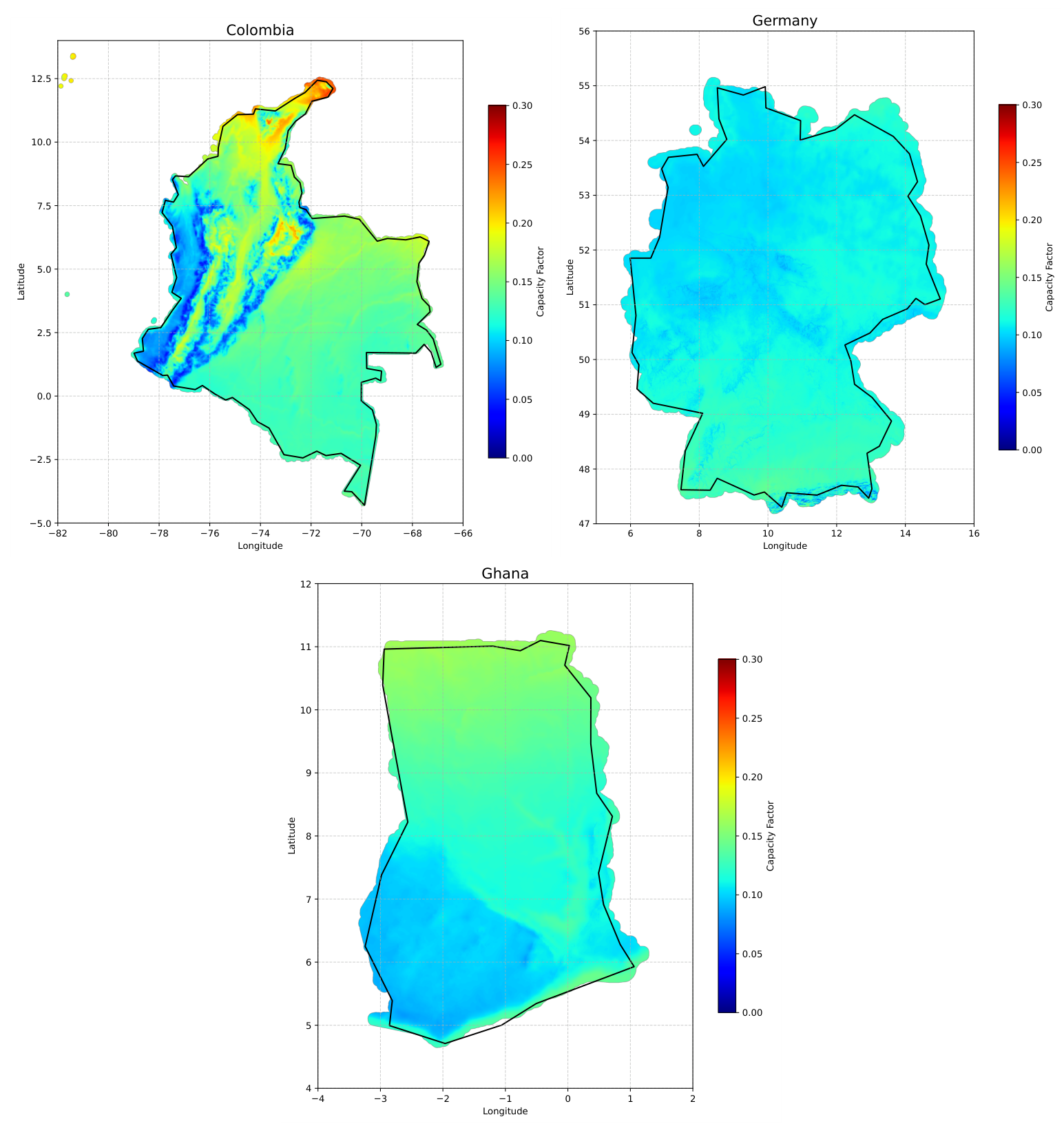
Figure 1. Geographical distribution of solar capacity factor CF for Colombia, Germany, and Ghana.
Technologies 14 00593 g001
Figure 2. Geographical distribution of wind CF for Colombia, Germany, and Ghana.
Technologies 14 00593 g002
Figure 3. Sensitivity of TDI, C F r e a l and carbon footprint to parameter weight variations across Germany, Colombia, and Ghana.
Technologies 14 00593 g003
Figure 4. Human development index (HDI) by regions.
Technologies 14 00593 g004
Figure 5. Index of reliability and quality of the electricity infrastructure (INF) by regions.
Technologies 14 00593 g005
Figure 6. Normalized global innovation index (GII) by regions.
Technologies 14 00593 g006
Figure 7. Renewable energy readiness index (RERI) by regions.
Technologies 14 00593 g007
Figure 8. Technological development index (TDI) by regions.
Technologies 14 00593 g008
Figure 9. Capacity factor vs. H C r e a l for solar energy applications in the three studied countries.
Technologies 14 00593 g009
Figure 10. Capacity factor vs. H C r e a l for wind energy applications in the three studied countries.
Technologies 14 00593 g010
Table 1. Relative contribution of each life cycle stage to the carbon footprint (g CO2e/kWh) by renewable technology.
TechnologyManufacturingConstruction/
Installation
OperationMaintenanceDecommissioning/
Recycling
Estimated Total (g CO2e/kWh)Reference
Solar PV utility25–3510<11540–60[28,29,30,31,32]
On-shore wind utility∼7–11∼1–2<10.5–1.51–210–20[29,30,31,32,33]
Table 2. Typical rated wind speeds for different wind turbine classes.
Type of Wind TurbineRated Wind Speed ( v nom )Reference
Small turbines (<100 kW)≈8–11 m/s[45]
Medium turbines (100 kW to 1 MW)≈10–12 m/s[46]
Large turbines (>1 MW, IEC class I or II)≈11–13 m/s[47,48]
Turbines for moderate wind sites (IEC class III)≈8–10 m/s[47,48]
Table 3. Comparative analysis of the carbon footprint of solar PV technology in Germany, Colombia, and Ghana.
Country HC
(g CO2e/kWh)
Real Capacity
Factor (%)
Tech. Development
Index
HC real
(g CO2e/kWh)
Colombia52.080.1260.60650.89
Germany52.040.1040.76861.93
Ghana52.130.1000.33364.29
Table 4. Comparative analysis of the carbon footprint of on-shore wind technology in Germany, Colombia, and Ghana.
Country HC
(g CO2e/kWh)
Real Capacity
Factor (%)
Tech. Development
Index
HC real
(g CO2e/kWh)
Colombia17.610.1440.60620.76
Germany17.560.2540.76811.74
Ghana17.690.0670.33345.13
Disclaimer/Publisher’s Note: The statements, opinions and data contained in all publications are solely those of the individual author(s) and contributor(s) and not of MDPI and/or the editor(s). MDPI and/or the editor(s) disclaim responsibility for any injury to people or property resulting from any ideas, methods, instructions or products referred to in the content.