Relation-Consistency Group Contrastive Learning for Robust Multispectral Remote Sensing Classification

Abstract

Multispectral remote sensing classification benefits from the complementary information carried by visible (VIS), near-infrared (NIR), and short-wave infrared (SWIR) Sentinel-2 bands, yet most deep models process them as a single stacked tensor without explicitly preserving their inter-group relationships. We propose Relation-Consistency Group Contrastive Learning (Group-CL-RC), a robustness-oriented framework combining group-level contrastive alignment with a relation-consistency regularizer defined over a compact VIS–NIR–SWIR similarity descriptor. The method is evaluated on EuroSAT All Bands using four backbones under radiometric drift, spatial masking, K-drop band removal, and compound spectral–spatial corruption (CS2C), and externally validated on Sentinel-2-only SEN12MS under standard and seasonal-shift protocols. Group-CL-RC preserves strong clean performance and yields statistically supported robustness gains over the multispectral-only baseline, with the largest improvements under K-drop and CS2C. SEN12MS supports the transfer of these robustness trends beyond EuroSAT, while showing that gains over standard Group-CL remain perturbation-dependent. Ablation studies further indicate that relation consistency is an effective robustness mechanism, particularly when spectral-group availability is degraded. Relation-deformation diagnostics show that Group-CL-RC primarily reduces decision-level sensitivity to relational distortions rather than uniformly minimizing raw deformation. Overall, inter-group relational geometry provides an interpretable and effective robustness target under controlled structured spectral and spectral–spatial degradation.

1. Introduction

Multispectral Earth observation imagery has become a fundamental resource for large-scale environmental monitoring, land-cover mapping, agricultural assessment, and urban analysis. Modern satellite missions such as Sentinel-2 acquire images across several spectral bands spanning the visible (VIS), near-infrared (NIR), and short-wave infrared (SWIR) regions of the electromagnetic spectrum [1]. These spectral bands provide complementary information about land surfaces: visible bands capture color and fine spatial texture, near-infrared bands respond to vegetation vigor and biomass-related surface properties, and short-wave infrared bands are sensitive to moisture content, soil properties, and material composition. Effectively exploiting this cross-spectral complementarity remains a central challenge in multispectral remote sensing classification.

Despite substantial progress in deep learning for remote sensing, most multispectral classification pipelines still process spectral bands as uniformly stacked channels. This channel-stacking paradigm is practical and often effective, but it does not explicitly represent the physical organization of multispectral data or the relationships among semantically meaningful spectral subsets. This limitation is important because multispectral bands are not interchangeable measurements. Their organization reflects both sensor design and the physical interaction between electromagnetic radiation and land-surface materials [2]. In Sentinel-2 imagery, VIS, NIR, and SWIR bands encode distinct but complementary surface properties, and such physical distinctions are already widely exploited in remote sensing indices such as vegetation and moisture-related indices [3,4]. When all bands are processed uniformly, the learned representation may obscure this internal spectral structure. As a result, a model may learn discriminative features under clean conditions while remaining fragile when specific spectral groups are degraded, missing, or distorted.

Robustness is therefore a critical issue for operational multispectral remote sensing. In practical Earth observation pipelines, spectral measurements may be affected by sensor calibration drift, atmospheric effects, spatial-resolution inconsistencies across bands, missing channels, cloud contamination, shadows, or other sources of partial spectral degradation [2]. Clean test accuracy alone is thus insufficient to characterize model reliability. This concern is consistent with broader findings in computer vision showing that high clean accuracy does not necessarily imply robustness under common corruptions or distribution shift [5]. In multispectral land-cover classification, robustness is particularly challenging because corruptions are often structured rather than uniform: some perturbations modify radiometric statistics, whereas others suppress spatial regions or remove specific spectral groups. Such perturbations can disrupt not only individual band responses, but also the complementarity among spectral groups.

This observation motivates the central hypothesis of this work: robust multispectral representation learning should preserve not only group-specific embeddings, but also the relational geometry among physically meaningful spectral groups. From this perspective, multispectral robustness is partly a relational problem. The objective is therefore not merely to align spectral groups independently, but to learn a representation whose classification behavior is less sensitive to perturbation-induced deformations of the internal VIS–NIR–SWIR similarity structure. This relational viewpoint differs from standard channel-stacking classifiers, generic contrastive objectives, semantic supervision alone, and attention-based spectral fusion. Channel-stacking classifiers do not explicitly expose the physical organization of the multispectral signal. Standard group-level contrastive learning encourages compatibility among spectral-group embeddings, but it does not directly regularize the geometry of the full inter-group relation structure. Attention-based spectral fusion can learn to emphasize or suppress channels and branches, but it does not explicitly promote stability of cross-spectral relationships under degradation. Similarly, class-aware semantic losses encourage discriminative and compact class representations, whereas relation consistency targets the stability and decision-level usefulness of the cross-spectral structure itself.

To address this gap, we introduce Relation-Consistency Group Contrastive Learning (Group-CL-RC), a robustness-oriented multispectral representation-learning framework for Sentinel-2 image classification. The proposed method starts from structured spectral grouping and group-level contrastive alignment, but extends this formulation by regularizing the relational descriptor induced by VIS, NIR, and SWIR group embeddings. Rather than enforcing only pairwise spectral-group alignment, Group-CL-RC regularizes the inter-group similarity structure across clean and corrupted views. In this way, the method directly targets a failure mode that is particularly relevant under spectral degradation: deformation of the cross-spectral relational structure and its impact on the final classification decision.

The proposed framework is evaluated on EuroSAT All Bands [6] under both clean and robustness-oriented conditions. The robustness protocol covers four structured perturbation families: radiometric drift, spatial masking, K-drop band removal, and compound spectral–spatial corruption. To contextualize Group-CL-RC against representative external learning objectives, we further add a matched EuroSAT comparison with corruption-training and contrastive baselines implemented under the same experimental pipeline. External validation is then conducted on Sentinel-2-only SEN12MS under standard and seasonal-shift protocols [7].

The results show that Group-CL-RC preserves strong clean performance while improving robustness over the multispectral-only baseline under structured spectral and spectral–spatial degradation. The strongest gains occur when spectral-group availability or cross-spectral complementarity is disrupted, especially under K-drop and compound corruption. The comparison with standard Group-CL and the matched external baselines supports a conservative interpretation: relation consistency is most beneficial in specific degradation regimes and should be viewed as an interpretable robustness mechanism rather than as a universally dominant training strategy. Objective-component, descriptor-granularity, training-time corruption, relation-deformation, qualitative, and computational analyses are included to clarify the scope, reliability, and practical behavior of the proposed framework.

The main contributions of this work are summarized as follows:

• We formulate robustness-oriented multispectral representation learning as a problem of preserving inter-group relational geometry among physically meaningful spectral groups. This shifts the focus from embedding-level stability alone to the stability and decision-level usefulness of the internal VIS–NIR–SWIR structure under spectral degradation.
• We introduce Relation-Consistency Group Contrastive Learning (Group-CL-RC), a structured representation-learning framework that combines group-level contrastive alignment with a relation-consistency regularizer. The proposed regularizer promotes preservation of the similarity structure among VIS, NIR, and SWIR group embeddings across clean and corrupted views.
• We distinguish relation consistency from standard semantic supervision, generic spectral fusion, and pairwise contrastive alignment. The proposed mechanism targets the structural stability of cross-spectral relationships rather than only class compactness, channel reweighting, or feature-level agreement.
• We evaluate the framework under clean and robustness-oriented settings using Sentinel-2 EuroSAT All Bands, multiple backbone architectures, and four structured perturbation families: drift, masking, K-drop band removal, and compound spectral–spatial corruption. We further provide a matched external-baseline comparison with representative corruption-training and contrastive objectives, together with Sentinel-2-only SEN12MS validation under standard and seasonal-shift protocols.
• We conduct controlled ablation studies of the objective components, relation-descriptor granularity, and training-time corruption strategy. These analyses clarify when relation consistency contributes most, how descriptor complexity affects robustness and cost, and whether the training corruption design influences the observed robustness behavior.
• We provide diagnostic analyses showing that relation consistency reduces the decision-level sensitivity of the classifier to relation deformation, rather than merely minimizing raw relation-deformation magnitude. We also report computational profiling and qualitative prediction examples to characterize the practical overhead and observable effects of structured multispectral perturbations.

The remainder of this paper is organized as follows. Section 2 reviews related work on multispectral classification, robustness, contrastive learning, and relational representation learning. Section 3 presents the proposed Group-CL-RC framework and its optimization objectives. Section 4 describes the datasets, model variants, backbone architectures, training protocol, robustness perturbations, evaluation metrics, statistical testing, computational profiling, and reporting strategy. Section 5 reports the experimental results. Section 6 discusses the main findings, the relation-consistency mechanism, practical implications, and limitations. Section 7 concludes the paper and outlines future research directions.

2. Related Work

2.1. Multispectral Image Classification

Multispectral image classification assigns semantic land-cover or land-use labels to satellite image patches acquired over multiple spectral bands. Classical approaches relied on handcrafted spectral features, vegetation indices, and traditional machine-learning classifiers such as support vector machines and random forests [8,9]. Deep learning has substantially improved remote sensing image classification by enabling models to learn hierarchical spatial–spectral representations directly from image data [10,11]. Benchmark datasets such as EuroSAT have played an important role in evaluating Sentinel-2 land-use and land-cover classification models [6]. Beyond EuroSAT, larger resources involving Sentinel-2 imagery have broadened the evaluation landscape: BigEarthNet provides a large-scale multi-label Sentinel-2 benchmark for remote sensing image understanding [12,13], whereas the Sentinel-2 component of SEN12MS provides georeferenced multispectral imagery across diverse geographic and seasonal conditions [7].

Residual networks, efficient convolutional models, and transformer-based architectures have also been widely adopted to improve feature extraction and long-range spatial modeling [14,15,16,17,18,19]. Recent multispectral classification studies have further explored stacking-based ensemble learning and seasonal spectral-feature modeling, illustrating the continuing relevance of machine-learning strategies for exploiting multispectral information in land-cover and crop-type classification [20,21]. Despite these advances, many multispectral classification pipelines still rely on stacked-band representations in which all spectral channels are processed jointly without explicitly modeling the physical organization of the multispectral signal. This design is effective for learning discriminative features, but it provides limited control over the relationships among physically meaningful spectral groups such as VIS, NIR, and SWIR. This motivates representation-learning methods that exploit not only the discriminative content of spectral measurements, but also the relational structure induced by complementary spectral groups.

2.2. Robustness to Spectral and Spatial Degradation

In remote sensing, robustness concerns arise under cross-sensor, cross-region, seasonal, and acquisition-condition shifts [22]. These shifts can modify both the spatial appearance of land-cover classes and the spectral signatures recorded by the sensor, making clean in-distribution accuracy insufficient to characterize operational reliability. A wide range of strategies has therefore been investigated, including data augmentation, domain adaptation, and architecture-level robustness improvements [22,23]. Recent remote-sensing work has also combined feature-level perturbations with consistency regularization and contrastive learning in semi-supervised semantic segmentation, showing that perturbation-aware objectives can complement conventional image-level augmentation [24]. In hyperspectral image analysis, robustness to band noise, band degradation, and missing-channel conditions has received particular attention, since the high spectral dimensionality of hyperspectral data makes models sensitive to band-level distortions [25].

Robustness-oriented evaluation is less standardized in multispectral land-cover classification, although multispectral degradations can also be structured rather than uniform. Such degradations may selectively affect radiometric responses, spatial support, or specific spectral groups, and spectral and spatial perturbations may interact when they occur jointly. This structure matters because a model that remains stable under broad image-level perturbations may still be vulnerable when degradation affects the bands or spectral groups carrying class-discriminative information. Robustness analysis in multispectral classification should therefore distinguish radiometric, spatial, spectral, and compound degradation modes instead of treating corruption as a single uniform condition.

2.3. Spectral–Spatial Fusion and Attention

Several research directions have sought to improve multispectral and hyperspectral representation learning through stronger backbones, spectral–spatial fusion modules, band selection, and attention mechanisms. These approaches exploit the complementary nature of spatial context and spectral information by improving feature extraction, aggregation, and adaptive spectral weighting. Spectral–spatial architectures and attention mechanisms have been particularly influential in hyperspectral image analysis, where dense spectral sampling makes it important to capture both local spatial patterns and dependencies across bands [26,27]. For Sentinel-2-based semantic segmentation of offshore floating raft aquaculture areas, MSSFNet combines a spatial–spectral feature extraction block with a multiscale spatial attention block, illustrating the value of jointly exploiting complementary spectral and multiscale spatial information [28].

Although effective for selecting and combining informative spectral cues, these methods are generally not designed to regularize the stability of relationships among physically meaningful spectral groups under degradation. Structured perturbations may affect not only individual band features, but also the cross-spectral relationships implicitly used by the classifier. Fusion- and attention-based approaches can therefore be complemented by representation-learning objectives that explicitly regularize inter-group spectral relationships.

2.4. Contrastive Representation Learning in Remote Sensing

Contrastive representation learning has become an important paradigm for learning invariant and transferable visual representations. Methods such as SimCLR and MoCo learn representations by bringing augmented views of the same sample closer while separating unrelated samples [29,30], whereas BYOL showed that view consistency can also be exploited without explicit negative pairs [31]. Supervised contrastive learning further incorporates label information into the contrastive objective [32], and CLIP demonstrated the effectiveness of large-scale contrastive alignment across heterogeneous modalities [33].

In remote sensing, contrastive learning has been adapted to exploit geospatial structure, spatial context, multimodal Earth observation data, and geography-aware self-supervision [34,35,36]. Recent studies have additionally applied contrastive learning to multispectral band-aware cross-domain satellite image generation [37], while joint cluster- and instance-level contrastive learning developed primarily for aerial person re-identification has also been evaluated on remote-sensing classification datasets [38]. Recent Earth observation pretraining and foundation-model studies have further extended contrastive objectives toward multimodal, multi-granularity, and label-guided representation learning [39,40]. These developments are important because remote sensing images often provide multiple complementary views of the same location, whether through augmentations, temporal observations, sensor modalities, or spectral subsets. For multispectral imagery, physically meaningful spectral groups can therefore be interpreted as complementary views of the same scene, motivating group-level contrastive alignment among spectral subsets such as VIS, NIR, and SWIR.

However, standard contrastive formulations primarily operate at the level of individual samples, views, modalities, or pairwise embeddings. They encourage agreement between related representations, but they do not explicitly preserve the relational structure jointly induced by multiple spectral groups. Pairwise alignment among VIS, NIR, and SWIR embeddings therefore does not guarantee that their mutual similarity geometry remains stable when specific bands or spectral groups are corrupted. This motivates relation-aware objectives that complement contrastive alignment by regularizing the inter-group structure itself.

2.5. Relational Representation Learning

Relational representation learning offers a complementary viewpoint by focusing on the structure of relationships among embeddings rather than only on the embeddings themselves. In self-supervised learning, relational reasoning has been used to exploit dependencies among observations and to preserve similarity structures across views [41,42]. Related ideas have also been explored in relation-preserving knowledge distillation, where mutual distances, angles, or activation-similarity patterns among examples are transferred between models [43,44]. Metric-learning formulations have further modeled higher-order dependencies beyond direct pairwise distances [45]. These studies indicate that representation quality may depend not only on individual embedding positions, but also on the geometry of their relations.

However, most existing relational formulations operate across instances, teacher–student representations, or generic feature ensembles. They are not specifically designed to model the physically grounded relationships among spectral groups within a single multispectral sample, nor to preserve these relationships under structured spectral and spectral–spatial degradation. This distinction is important for multispectral imagery because VIS, NIR, and SWIR groups correspond to physically meaningful wavelength regions and encode complementary surface information. A robustness-oriented multispectral representation may therefore benefit from preserving the relationships among these group representations when the input is degraded. The remaining gap is therefore to model inter-group spectral relations as an explicit object of regularization under degradation, rather than relying only on individual embeddings, pairwise alignment, or generic feature fusion.

3. Materials and Methods

This section presents the proposed Relation-Consistency Group Contrastive Learning framework, denoted as Group-CL-RC. The method builds structured VIS, NIR, and SWIR spectral views from a Sentinel-2 multispectral input, learns group-compatible embeddings, and regularizes the relation descriptor induced by these groups under degradation. We describe the model formulation, spectral grouping, shared encoder, fusion branch, group-level contrastive objective, relation-consistency regularizer, and final optimization objective.

3.1. Overview of the Proposed Framework

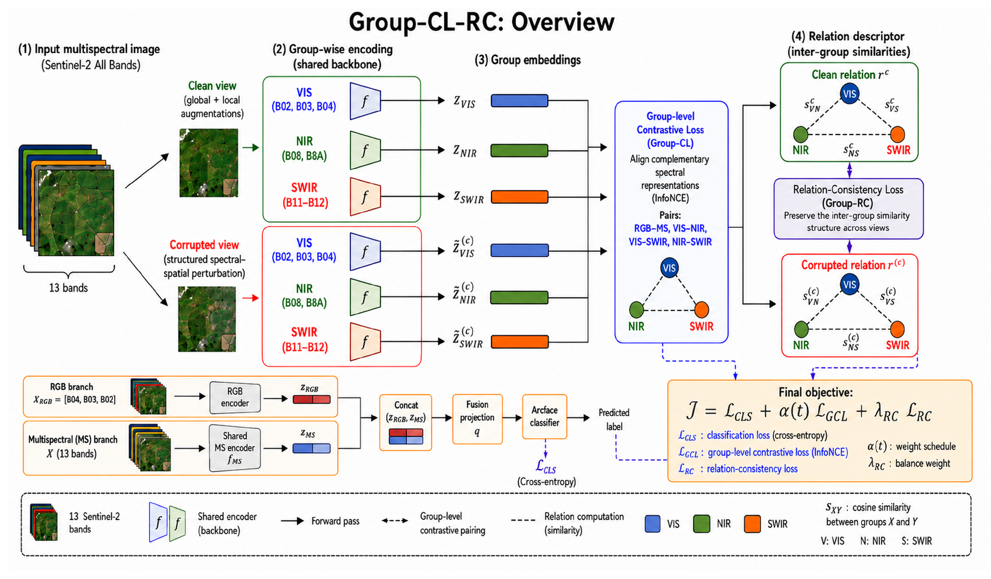
Given a Sentinel-2 multispectral image, Group-CL-RC constructs a full multispectral representation and group-specific representations for the VIS, NIR, and SWIR spectral regions. A shared multispectral encoder processes both the full input and the masked group-specific views, while a separate RGB branch provides visible-spectrum features for the final fused classifier. Group-level contrastive learning promotes compatibility among complementary spectral views, and relation-consistency regularization preserves the VIS–NIR–SWIR similarity structure between clean and degraded views.

The framework contains four main components:

• A spectral-group decomposition that defines VIS, NIR, and SWIR group views from the original multispectral image;
• A shared multispectral encoder and projection head that map full and group-specific inputs into a common embedding space;
• A fusion and classification branch that combines visible-spectrum and full multispectral representations for land-cover prediction;
• A robustness-oriented training objective that combines group-level contrastive alignment with relation-consistency regularization.

The contrastive and relation-consistency objectives are used only as training-time auxiliary regularizers. At inference time, the final prediction is produced by the fused RGB–MS classification branch.

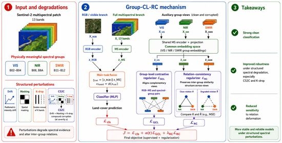
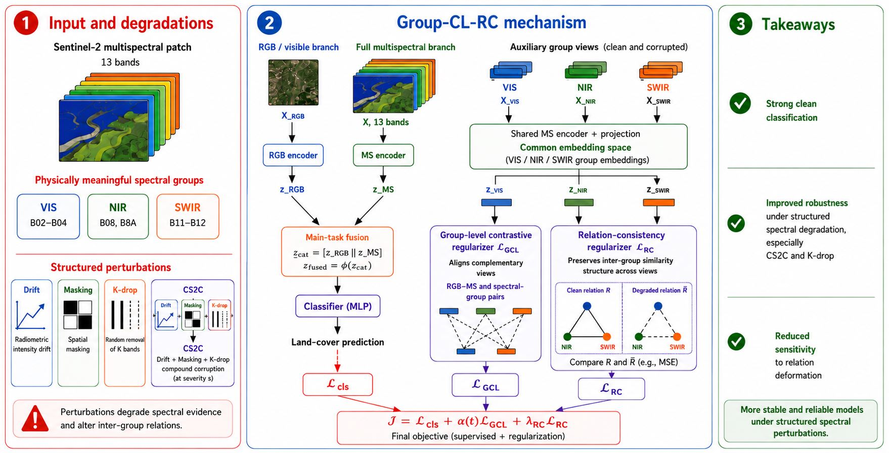
Figure 1 provides a visual summary of the proposed Group-CL-RC framework. The diagram highlights the interaction between group-level contrastive alignment, relation-consistency regularization, and supervised classification within the overall robustness-oriented learning objective.

3.2. Problem Formulation

Let $X\in {\mathbb{R}}^{C\times H\times W}$ denote a multispectral image, where C is the number of spectral bands and $H\times W$ is the spatial resolution. In the EuroSAT All Bands setting, X corresponds to a Sentinel-2 multispectral image patch with $C=13$ spectral channels. In the SEN12MS external validation setting, the same formulation is used with $C=10$ retained Sentinel-2 bands. Each image has a land-cover label $y\in \{1,\dots ,K\}$, where K is the number of classes.

A standard multispectral classifier learns an encoder

$$f_{\theta }:{\mathbb{R}}^{C\times H\times W}\to {\mathbb{R}}^{d_b},$$

(1)

followed by a prediction module that maps the extracted representation to class logits. Most multispectral deep learning pipelines process X as a single stacked spectral tensor, in which all bands are treated as input channels of the same representation. Although effective, this formulation does not explicitly encode the physical organization of the multispectral signal or the relationships among spectral groups.

Let ${\tilde{X}}^{\left(c\right)}$ denote a degraded version of X produced by a structured perturbation operator $c\in \mathcal{C}$. In this setting, a robust multispectral representation should satisfy three properties. First, the learned representation should remain discriminative for land-cover classification. Second, embeddings associated with complementary spectral groups should remain compatible in the latent space. Third, the relational geometry among physically meaningful spectral groups should remain sufficiently stable under degradation so that perturbation-induced changes in cross-spectral structure have limited impact on the final prediction.

3.3. Spectral Group Decomposition

We define three physically meaningful spectral groups:

$$\mathcal{G}=\{\mathrm{VIS},\mathrm{NIR},\mathrm{SWIR}\}.$$

(2)

The grouping used in this work is:

$$\mathrm{VIS}=\{B02,B03,B04\},\mathrm{NIR}=\{B08,B8A\},\mathrm{SWIR}=\{B11,B12\}.$$

(3)

The VIS group corresponds to the blue, green, and red Sentinel-2 bands and represents visible-spectrum information. The NIR group is associated with vegetation reflectance, while the SWIR group provides complementary information about moisture content, soil properties, and material composition. The RGB branch uses the same visible bands as VIS, but ordered as B04, B03, and B02 to form a conventional RGB input. The VIS, NIR, and SWIR groups are used to construct the relation-consistency descriptor, while the remaining available Sentinel-2 bands are retained in the full multispectral input. This grouping is valid for both datasets used in this study: EuroSAT All Bands provides a 13-band Sentinel-2 input, whereas the SEN12MS external validation uses the ten retained Sentinel-2 bands available in our setting. In both cases, the VIS, NIR, and SWIR bands required by the default relation descriptor are present.

For each group $g\in \mathcal{G}$, we define a deterministic masking operator

$$M_g:{\mathbb{R}}^{C\times H\times W}\to {\mathbb{R}}^{C\times H\times W},$$

(4)

which preserves the channels belonging to group g and sets the remaining channels to zero. The group-specific view is then given by

$$X_g=M_g\left(X\right),g\in \mathcal{G}.$$

(5)

This construction preserves a common input dimensionality for the full multispectral image and all group-specific views, allowing the same multispectral encoder to process both complete and masked inputs. Bands outside the default VIS, NIR, and SWIR groups, including red-edge and atmospheric bands, remain available through the full multispectral branch. They are not used as separate groups in the default relation descriptor, in order to avoid over-fragmenting the spectral space and to keep the main formulation focused on three broad spectral regimes. A finer red-edge-aware grouping is evaluated separately in the descriptor-granularity ablation.

3.4. Shared Multispectral Encoder for Full and Group-Specific Views

Let $f_{\mathrm{MS}}$ denote the multispectral encoder:

$$f_{\mathrm{MS}}:{\mathbb{R}}^{C\times H\times W}\to {\mathbb{R}}^{d_b},$$

(6)

where $d_b$ is the backbone feature dimension. The encoder can be instantiated with different backbone architectures, such as ResNet-50, EfficientNet-B0, ConvNeXt-Tiny, or Swin-Tiny. The number of input channels is dataset-specific: $C=13$ for EuroSAT All Bands and $C=10$ for the Sentinel-2-only SEN12MS external validation. Accordingly, the multispectral input stem or patch embedding is instantiated for the corresponding number of Sentinel-2 bands, while the same VIS–NIR–SWIR relation-consistency definition is retained.

Given the full multispectral image X, the encoder produces the backbone feature:

$$h_{\mathrm{MS}}=f_{\mathrm{MS}}\left(X\right).$$

(7)

A projection head P maps backbone features to a common d-dimensional embedding space:

$$P:{\mathbb{R}}^{d_b}\to {\mathbb{R}}^d.$$

(8)

The full multispectral embedding is therefore defined as:

$$z_{\mathrm{MS}}=P\left(h_{\mathrm{MS}}\right)=P\left(f_{\mathrm{MS}}\left(X\right)\right).$$

(9)

For each spectral group $g\in \mathcal{G}$, the group-specific view $X_g$ is passed through the same multispectral encoder and the same projection head:

$$h_g=f_{\mathrm{MS}}\left(X_g\right),$$

(10)

$$z_g=P\left(h_g\right)=P\left(f_{\mathrm{MS}}\left(M_g\left(X\right)\right)\right).$$

(11)

This weight-sharing design avoids introducing separate encoders for individual spectral groups and places the full and masked inputs in a common latent space. The group-specific embeddings are used only as auxiliary training representations for the contrastive and relation-consistency objectives.

The final land-cover prediction is not made from individual masked group views, but from the fused representation defined in Section 3.5.

3.5. Fusion Representation and Classification Head

The final supervised decision is made from a fused representation that combines visible-spectrum and multispectral information. Let $X_{\mathrm{RGB}}\in {\mathbb{R}}^{3\times H\times W}$ denote the RGB subset formed by Sentinel-2 bands $B04$, $B03$, and $B02$. An RGB encoder $f_{\mathrm{RGB}}$ extracts visible-spectrum features:

$$h_{\mathrm{RGB}}=f_{\mathrm{RGB}}\left(X_{\mathrm{RGB}}\right).$$

(12)

The RGB embedding is obtained through a projection head $P_{\mathrm{RGB}}$:

$$z_{\mathrm{RGB}}=P_{\mathrm{RGB}}\left(h_{\mathrm{RGB}}\right).$$

(13)

The full multispectral embedding $z_{\mathrm{MS}}$ and the RGB embedding $z_{\mathrm{RGB}}$ are concatenated:

$$z_{\mathrm{cat}}=\mathrm{Concat}(z_{\mathrm{RGB}},z_{\mathrm{MS}}).$$

(14)

The fused representation is then obtained through a lightweight projection module $\varphi$:

$$z_{\mathrm{fused}}=\varphi \left(z_{\mathrm{cat}}\right).$$

(15)

In the implementation used in this work, $\varphi$ is a multilayer perceptron with a nonlinear activation. The fused representation is used for supervised land-cover classification, while the group-specific embeddings serve only the auxiliary contrastive and relation-consistency objectives.

The supervised classification loss is based on ArcFace, an angular-margin objective that encourages discriminative separation on the hypersphere [46]. Let ${\tilde{z}}_i$ denote the ${\mathsf{\ell }}_2$-normalized fused representation of sample i:

$${\tilde{z}}_i={\displaystyle \frac{z_{\mathrm{fused},i}}{\parallel z_{\mathrm{fused},i}{\parallel }_2}}.$$

(16)

Let $W=[w_1,\dots ,w_K]$ denote the class-prototype matrix, with normalized class prototypes $\parallel w_k{\parallel }_2=1$. The cosine similarity between sample i and class k is:

$$\cos \left({\theta }_{i,k}\right)=w_k^{\top }{\tilde{z}}_i.$$

(17)

ArcFace introduces an additive angular margin m for the ground-truth class:

$${\mathsf{\ell }}_{i,k}=\left\{\begin{array}{cc}s·\cos ({\theta }_{i,y_i}+m),\hfill & \mathrm{if}k=y_i,\hfill \\ s·\cos \left({\theta }_{i,k}\right),\hfill & \mathrm{otherwise},\hfill \end{array}\right.$$

(18)

where s is a scale parameter. The classification loss is the cross-entropy over these margin-modified logits:

$${\mathcal{L}}_{\mathrm{cls}}=-{\displaystyle \frac{1}{N}}{\displaystyle \sum _{i=1}^N}log{\displaystyle \frac{\exp \left({\mathsf{\ell }}_{i,y_i}\right)}{{\sum }_{k=1}^K\exp \left({\mathsf{\ell }}_{i,k}\right)}}.$$

(19)

3.6. Group-Level Contrastive Learning

The classification objective encourages semantic discrimination but does not explicitly enforce compatibility among complementary spectral views of the same scene. To address this limitation, we use a group-level contrastive objective over physically meaningful spectral representations and the visible-spectrum/multispectral branch structure.

Let $z_a^i$ and $z_b^i$ denote two embeddings extracted from the same image i, where a and b refer to two representation branches or spectral groups. In the proposed Group-CL-RC framework, the active contrastive pairs are RGB–MS, VIS–NIR, VIS–SWIR, and NIR–SWIR. The RGB–MS term encourages compatibility between the visible branch and the full multispectral branch, whereas the VIS–NIR, VIS–SWIR, and NIR–SWIR terms encourage compatibility among physically meaningful spectral groups.

Similarity is computed using cosine similarity:

$$\mathrm{sim}(z_a,z_b)={\displaystyle \frac{z_a^{\top }{z}_b}{\parallel z_a{\parallel }_2{\parallel z_b\parallel }_2}}.$$

(20)

For a contrastive pair $(a,b)$, the InfoNCE loss is defined as:

$${\mathcal{L}}_{a,b}=-{\displaystyle \frac{1}{N}}{\displaystyle \sum _{i=1}^N}log{\displaystyle \frac{\exp (\mathrm{sim}(z_a^i,z_b^i)/\tau )}{{\sum }_{j=1}^N\exp (\mathrm{sim}(z_a^i,z_b^j)/\tau )}},$$

(21)

where N is the batch size and $\tau$ is the temperature parameter.

The group-level contrastive loss is written as the following weighted sum:

$$\begin{array}{cc}\hfill {\mathcal{L}}_{\mathrm{GCL}}=& {\lambda }_{\mathrm{RGB},\mathrm{MS}}{\mathcal{L}}_{\mathrm{RGB},\mathrm{MS}}+{\lambda }_{\mathrm{VIS},\mathrm{NIR}}{\mathcal{L}}_{\mathrm{VIS},\mathrm{NIR}}\hfill \\ \hfill & +{\lambda }_{\mathrm{VIS},\mathrm{SWIR}}{\mathcal{L}}_{\mathrm{VIS},\mathrm{SWIR}}+{\lambda }_{\mathrm{NIR},\mathrm{SWIR}}{\mathcal{L}}_{\mathrm{NIR},\mathrm{SWIR}}.\hfill \end{array}$$

(22)

The pair-specific weights ${\lambda }_{\mathrm{RGB},\mathrm{MS}}$, ${\lambda }_{\mathrm{VIS},\mathrm{NIR}}$, ${\lambda }_{\mathrm{VIS},\mathrm{SWIR}}$, and ${\lambda }_{\mathrm{NIR},\mathrm{SWIR}}$ are specified by the corresponding backbone configuration. This pair-weighted formulation allows the strength of each spectral-pair constraint to be controlled separately.

During training, the contribution of ${\mathcal{L}}_{\mathrm{GCL}}$ is modulated by a warm-up/ramp-up factor $\alpha \left(t\right)$, where t denotes the epoch:

$$\alpha \left(t\right)=\left\{\begin{array}{cc}0,\hfill & t\le T_{\mathrm{warm}},\hfill \\ \min \left(1,{\displaystyle \frac{t-T_{\mathrm{warm}}}{T_{\mathrm{ramp}}}}\right),\hfill & t>T_{\mathrm{warm}}.\hfill \end{array}\right.$$

(23)

Here, $T_{\mathrm{warm}}$ is the number of warm-up epochs during which the contrastive contribution is disabled, and $T_{\mathrm{ramp}}$ is the number of ramp-up epochs used to progressively introduce the contrastive loss. This schedule prevents the contrastive objective from dominating the early supervised optimization stage.

Thus, ${\mathcal{L}}_{\mathrm{GCL}}$ promotes embedding-level compatibility among selected spectral views. The next subsection introduces a complementary regularizer that acts on the joint VIS–NIR–SWIR relation structure under degradation.

3.7. Relation-Consistency Regularization

Group-level contrastive learning encourages pairwise compatibility between selected spectral embeddings, but it does not explicitly constrain the joint relational geometry formed by the VIS, NIR, and SWIR groups. Group-CL-RC therefore introduces a relation-consistency regularizer that operates on a compact inter-group similarity descriptor.

For a clean multispectral image X, the default descriptor is built from the three pairwise similarities among VIS, NIR, and SWIR embeddings:

$$R\left(X\right)=\left[\begin{array}{c}\mathrm{sim}(z_{\mathrm{VIS}},z_{\mathrm{NIR}})\\ \mathrm{sim}(z_{\mathrm{VIS}},z_{\mathrm{SWIR}})\\ \mathrm{sim}(z_{\mathrm{NIR}},z_{\mathrm{SWIR}})\end{array}\right]\in {\mathbb{R}}^3.$$

(24)

This descriptor summarizes the internal similarity configuration among the three physically meaningful spectral-group embeddings. It is not a class prediction and is not used as an additional classifier output. The descriptor is intentionally compact: with three spectral groups, the three pairwise similarities form the complete set of first-order inter-group relations. This avoids additional graph, covariance, or attention-based design choices while keeping the relation-consistency mechanism interpretable and architecture-agnostic. A finer red-edge-aware descriptor is evaluated separately in the descriptor-granularity ablation, whereas the default framework uses the VIS–NIR–SWIR descriptor.

Let ${\tilde{X}}^{\left(c\right)}$ denote a degraded view of X generated by a structured corruption operator c. For each group $g\in \mathcal{G}$, the corrupted group view is obtained by applying the same masking operator to the degraded multispectral image:

$${\tilde{X}}_g^{\left(c\right)}=M_g({\tilde{X}}^{\left(c\right)}).$$

(25)

The corresponding group embedding is

$${\tilde{z}}_g^{\left(c\right)}=P\left(f_{\mathrm{MS}}({\tilde{X}}_g^{\left(c\right)})\right).$$

(26)

The relation descriptor of the degraded view is then defined analogously:

$$R({\tilde{X}}^{\left(c\right)})=\left[\begin{array}{c}\mathrm{sim}({\tilde{z}}_{\mathrm{VIS}}^{\left(c\right)},{\tilde{z}}_{\mathrm{NIR}}^{\left(c\right)})\\ \mathrm{sim}({\tilde{z}}_{\mathrm{VIS}}^{\left(c\right)},{\tilde{z}}_{\mathrm{SWIR}}^{\left(c\right)})\\ \mathrm{sim}({\tilde{z}}_{\mathrm{NIR}}^{\left(c\right)},{\tilde{z}}_{\mathrm{SWIR}}^{\left(c\right)})\end{array}\right]\in {\mathbb{R}}^3.$$

(27)

The relation-consistency loss penalizes the discrepancy between the clean and degraded relation descriptors:

$${\mathcal{L}}_{\mathrm{RC}}={\displaystyle \frac{1}{N}}{\displaystyle \sum _{i=1}^N}{∥R\left(X_i\right)-R({\tilde{X}}_i^{\left(c\right)})∥}_2^2.$$

(28)

This objective differs from direct embedding alignment. It does not require each spectral-group embedding to remain unchanged under degradation. Instead, it regularizes the relative similarity configuration among spectral groups. The model is therefore encouraged to learn representations whose classification behavior is less sensitive to perturbation-induced changes in cross-spectral relational structure.

Relation consistency should not be interpreted as imposing strict invariance of the descriptor under every possible corruption. Some structured perturbations can legitimately alter spectral relationships. The goal is therefore not to force identical clean and corrupted descriptors in all cases, but to reduce the harmful effect of perturbation-induced relational distortions on the learned representation and final classification behavior. This distinction is examined empirically through the relation-deformation diagnostics reported in the experimental section.

3.8. Overall Training Objective

The proposed framework combines supervised classification, group-level contrastive alignment, and relation-consistency regularization. To avoid notation ambiguity, we denote by ${\mathcal{L}}_{\mathrm{GCL}}$ the weighted group-level contrastive loss defined over the active contrastive pairs, and by $\mathcal{J}$ the total optimization objective.

The multispectral-only baseline is trained using only the supervised classification loss:

$${\mathcal{J}}_{\mathrm{MS}}={\mathcal{L}}_{\mathrm{cls}}.$$

(29)

The Group-CL objective adds the group-level contrastive term:

$${\mathcal{J}}_{\text{Group-CL}}={\mathcal{L}}_{\mathrm{cls}}+\alpha \left(t\right){\mathcal{L}}_{\mathrm{GCL}},$$

(30)

where $\alpha \left(t\right)$ is the contrastive warm-up/ramp-up factor.

To isolate the contribution of relation consistency, we also consider a Group-RC objective:

$${\mathcal{J}}_{\text{Group-RC}}={\mathcal{L}}_{\mathrm{cls}}+{\lambda }_{\mathrm{RC}}{\mathcal{L}}_{\mathrm{RC}}.$$

(31)

This variant removes the contrastive term and is used as an objective-component ablation.

The proposed Group-CL-RC objective combines both auxiliary mechanisms:

$${\mathcal{J}}_{\text{Group-CL-RC}}={\mathcal{L}}_{\mathrm{cls}}+\alpha \left(t\right){\mathcal{L}}_{\mathrm{GCL}}+{\lambda }_{\mathrm{RC}}{\mathcal{L}}_{\mathrm{RC}}.$$

(32)

The three terms play complementary roles. The classification loss optimizes land-cover discrimination from the fused representation. The group-level contrastive loss promotes embedding-level compatibility among visible, multispectral, and spectral-group representations. The relation-consistency loss regularizes the VIS–NIR–SWIR descriptor between clean and training-time degraded views. In the default Group-CL-RC configuration, the degraded view is generated by a structured spectral corruption specified in the experimental setup.

The auxiliary objectives are used during training to shape the representation space. At inference time, prediction is made from the fused RGB–MS representation using the classification head; no additional relation descriptor or group-specific classifier is required for the final decision. This design keeps the inference-time decision pathway unchanged while using group-level and relation-level constraints to promote robustness under structured spectral and spectral–spatial degradation.

4. Experimental Setup

This section describes the datasets, model variants, training procedure, robustness perturbations, evaluation metrics, statistical analysis, computational profiling, and reproducibility settings used to evaluate Group-CL-RC.

4.1. Datasets and Preprocessing

The main experiments are conducted on EuroSAT All Bands, a Sentinel-2 multispectral land-use and land-cover classification dataset [6]. Each sample is a $64\times 64$ image patch assigned to one of ten semantic land-cover classes. In this setting, the full multispectral input uses the 13 Sentinel-2 bands available in EuroSAT All Bands. All inputs are normalized using dataset-level statistics to reduce inter-band scale differences and stabilize optimization. The same train, validation, and test splits, label mapping, and preprocessing pipeline are used across the clean, robustness, ablation, and diagnostic experiments on EuroSAT.

To assess whether the robustness behavior observed on EuroSAT extends beyond the main benchmark, we construct an external validation setting from SEN12MS [7]. SEN12MS is used only through its Sentinel-2 multispectral component; Sentinel-1 data are excluded and no multi-sensor fusion is performed. The retained SEN12MS Sentinel-2 input contains ten bands:

$$\{B02,B03,B04,B05,B06,B07,B08,B8A,B11,B12\}.$$

This 10-band configuration preserves all bands required by the default Group-CL-RC relation descriptor, namely VIS $=\{B02,B03,B04\}$, NIR $=\{B08,B8A\}$, and SWIR $=\{B11,B12\}$. The EuroSAT All Bands channels not retained in our SEN12MS input, namely $B01$, $B09$, and $B10$, are therefore absent from the SEN12MS validation input, but they are not required to construct the VIS–NIR–SWIR relation descriptor. This design keeps the external validation aligned with the Sentinel-2 multispectral setting and with the proposed relation-consistency framework, while adapting the full multispectral input dimensionality from 13 bands in EuroSAT to 10 bands in SEN12MS.

The SEN12MS label space is filtered to retain eight harmonized land-cover classes, corresponding to the class identifiers retained in the constructed manifests:

$$\{1,2,3,4,5,6,7,10\}.$$

Samples outside this retained class set are removed before constructing the final partitions. The retained class identifiers are then mapped consistently across training, validation, and test sets, so that all evaluated models solve the same eight-class classification problem. This filtering defines a controlled external validation setting rather than reproducing the full original SEN12MS label space.

Two SEN12MS validation protocols are constructed from the filtered Sentinel-2 samples. The first is a standard scene-disjoint protocol, in which the training, validation, and test partitions are built from disjoint scene sets. This prevents samples from the same scene from appearing simultaneously in training or validation and in the test set. The resulting standard protocol contains 13,200 training samples, 4420 validation samples, and 18,106 test samples. The second is a seasonal-shift protocol, in which non-winter scenes are used for training and validation, while winter scenes are reserved for testing. This protocol is designed to introduce a stronger seasonal distribution shift than the standard scene-disjoint setting and contains 13,089 training samples, 4331 validation samples, and 29,027 winter test samples.

For both SEN12MS protocols, the constructed data records preserve the sample identifier, scene identifier, season, and class label. These metadata fields make the scene-level and seasonal structure traceable during evaluation and ensure that the standard and seasonal-shift protocols remain distinguishable after inference. Both protocols use the same retained class set and the same Sentinel-2-only preprocessing convention; therefore, differences between them arise from the split construction rather than from the label space or sensor configuration. The SEN12MS protocols are used only as external validation settings and are reported separately from the EuroSAT experiments because SEN12MS differs from EuroSAT in spatial coverage, class taxonomy, sample distribution, and acquisition conditions.

The main characteristics of the two SEN12MS validation protocols are summarized in

Table 1. SEN12MS external validation protocols used in this study. Both protocols use the Sentinel-2 multispectral component only, retain ten Sentinel-2 bands, and retain eight harmonized land-cover classes.

Protocol	Train Samples	Validation Samples	Test Samples	Split Criterion
Standard scene-disjoint	13,200	4420	18,106	Disjoint scenes
Seasonal shift	13,089	4331	29,027	Non-winter to winter

.

4.2. Model Variants and Backbones

The evaluation compares four objective variants. The multispectral-only baseline, denoted as ms_only, uses the full multispectral input and is optimized only with the supervised classification objective. The group_cl variant adds group-level contrastive alignment without relation consistency. The group_rc variant uses relation-consistency regularization without group-level contrastive learning. The proposed Group-CL-RC variant combines supervised classification, group-level contrastive alignment, and relation-consistency regularization.

The main EuroSAT clean and robustness comparisons are conducted with four backbone architectures: ConvNeXt-Tiny [47], ResNet-50 [16], EfficientNet-B0 [17], and Swin-Tiny [15]. These backbones cover convolutional and transformer-based representation families and allow us to assess whether the robustness behavior of relation consistency is architecture-dependent. For all backbones, the multispectral input stem is adapted to the dataset-specific Sentinel-2 input dimensionality: 13 channels for EuroSAT All Bands and 10 channels for the SEN12MS external validation. The projection dimension is fixed to $d=256$ across the multispectral branch, RGB branch, group-specific embeddings, and fused representation.

Additional clean ablation variants are reported in Supplementary Section S1.2 and Supplementary Tables S11 and S12. They are used only to contextualize nominal performance and are not treated as main robustness baselines.

4.3. Training Protocol

All experiments follow a common training and evaluation pipeline. Training samples use the training transform, whereas validation and test samples use the deterministic evaluation transform. The best checkpoint is selected according to validation Macro-F1 and reloaded before final test evaluation.

Training uses AdamW with cosine annealing learning-rate scheduling. Automatic mixed precision, gradient clipping, learning rates, batch sizes, objective weights, and contrastive schedules are controlled by backbone-specific configuration files and reported in Supplementary Section S1.1 and Supplementary Tables S1–S10. For variants using ArcFace, the angular-margin head uses scale parameter $s=30.0$ and margin $m=0.2$ [46]. For variants using group-level contrastive learning, InfoNCE is used with temperature $\tau =0.07$.

For relation-consistency variants, training uses clean and corrupted views of the same input and evaluates the relation-consistency loss between their inter-group descriptors. In the default Group-CL-RC configuration, the corrupted training view is generated using K-drop band removal on the NIR + SWIR groups with $k=1$. This training-time corruption is distinct from the evaluation-time perturbations described in Section 4.4. Alternative training-time corruptions are examined in Section 5.8.

4.4. Robustness Perturbation Protocol

Robustness is evaluated using four structured perturbation families applied only at test time. They are not used as training labels or model-selection criteria, but as controlled stress tests for isolating different failure modes under spectral or spatial degradation.

Radiometric Drift

Radiometric drift applies gain, bias, and noise changes to selected spectral channels or spectral groups in order to evaluate sensitivity to radiometric instability. The evaluated drift levels use paired gain, bias, and noise values:

$$(0.00,0.00,0.000),(0.05,0.02,0.005),(0.10,0.03,0.010),(0.20,0.05,0.015).$$

Masking

Masking suppresses localized spatial regions with mask ratios $0.0$, $0.1$, $0.2$, and $0.3$, using patch sizes between 8 and 24 pixels. It evaluates the effect of local spatial unreliability in the multispectral input.

K-Drop Band Removal

K-drop removes a target-dependent number of spectral bands from selected spectral groups. It directly evaluates robustness to missing or unavailable spectral information, with particular relevance to non-visible spectral evidence.

Compound Spectral–Spatial Corruption

The compound spectral–spatial corruption family, denoted as CS2C, combines radiometric drift, spatial masking, resolution mismatch, band misregistration, and K-drop band removal within a single controlled degradation. It is designed to stress the classifier under simultaneous spectral and spatial distortions rather than under a single isolated perturbation. CS2C uses four ordinal severity levels indexed from 0 to 3, with the exact parameter schedule reported in

Table 2. Severity schedule used for compound spectral–spatial corruption (CS2C). The drift tuple denotes multiplicative gain, additive bias, and Gaussian noise standard deviation in scaled-reflectance space. The masking component uses random rectangular masks with patch sizes between 8 and 24 pixels. Resolution mismatch is implemented by downsampling and bilinear upsampling the selected bands. Misregistration denotes the maximum spatial shift, in pixels, applied to selected bands. The K-drop component removes k bands per sample from the selected target-band pool.

CS2C Severity	Drift $(\mathit{g},\mathit{b},\mathit{\sigma })$	Mask Ratio	Resolution Factor	Max. Shift	K-Drop k
0	$(0.00,0.00,0.000)$	$0.00$	1	0 px	0
1	$(0.05,0.02,0.005)$	$0.10$	2	1 px	0
2	$(0.10,0.03,0.010)$	$0.20$	2	2 px	1
3	$(0.20,0.05,0.015)$	$0.30$	3	2 px	2

. At each severity level, drift is applied in scaled-reflectance space, masking suppresses random rectangular spatial regions, resolution mismatch is simulated by downsampling and bilinear upsampling selected bands, misregistration spatially shifts selected bands, and K-drop removes a target-dependent number of bands from the selected target pool. Severity 0 corresponds to the unperturbed condition, whereas higher severities progressively increase the combined degradation. As for the other perturbation families, CS2C is used as a controlled stress test and should not be interpreted as an exhaustive simulation of all operational acquisition conditions.

The perturbations are evaluated on several spectral targets, including NIR, SWIR, NIR + SWIR, and non-RGB bands. The non-RGB target degrades non-visible spectral information while preserving the visible RGB channels. For CS2C, the selected target determines the bands affected by drift, masking, resolution mismatch, misregistration, and the band pool from which K-drop selects removed bands. Because perturbation families differ in severity and target structure, results are reported separately by corruption family. Additional severity-level and target-wise analyses are provided in Supplementary Sections S1.5 and S1.6, respectively.

4.5. Evaluation Metrics

The primary metric is Macro-F1, which gives equal importance to all classes and is suitable when robustness effects differ across land-cover categories. Accuracy is also reported for clean evaluation and selected robustness summaries as a standard reference metric.

For a given metric M, the family-level robustness gain of Group-CL-RC over the multispectral-only baseline is defined as

$$\Delta M_{\mathrm{avg}}=M_{\mathrm{avg}}^{\text{GCL-RC}}-M_{\mathrm{avg}}^{\mathrm{MS}},$$

(33)

where $M_{\mathrm{avg}}^{\text{GCL-RC}}$ and $M_{\mathrm{avg}}^{\mathrm{MS}}$ denote the average performances of Group-CL-RC and ms_only, respectively, over the matched evaluation points of a corruption family.

Worst-case robustness gain is defined as

$$\Delta M_{\mathrm{worst}}=M_{\mathrm{worst}}^{\text{GCL-RC}}-M_{\mathrm{worst}}^{\mathrm{MS}},$$

(34)

where $M_{\mathrm{worst}}^{\mathrm{GCL}-\mathrm{RC}}$ and $M_{\mathrm{worst}}^{\mathrm{MS}}$ denote the lowest performances observed within the corresponding corruption family.

For robustness-retention diagnostics, we also report the fraction of clean Macro-F1 preserved under non-clean perturbations. This metric complements absolute Macro-F1 by quantifying how much nominal performance is retained under degraded inputs.

4.6. Statistical Analysis

Results are reported as mean ± standard deviation over the relevant seeds, corruption instances, or matched evaluation grids, depending on the experimental block. The main clean comparison between ms_only and Group-CL-RC is reported over five seeds across four backbones. The main EuroSAT robustness comparison uses matched evaluation points, where each pair shares the same backbone, checkpoint seed, corruption family, target group, and perturbation level. This design isolates the effect of the model variant from variation in the robustness grid.

For inferential comparison blocks, paired statistical analyses are performed on matched evaluation points. For each inferential block, we report the mean paired difference, bootstrap confidence intervals, paired significance tests, Cohen’s $d_z$ when applicable, win/tie/loss counts, and Holm-corrected p-values for related comparison families. Statistical analyses are reported separately for the main EuroSAT robustness evaluation, SEN12MS external validation, objective-component ablation, descriptor-granularity ablation, and training-time corruption ablation.

The matched external-baseline comparison is reported as a descriptive controlled comparison over three seeds and the compact robustness grid. Since its purpose is to contextualize Group-CL-RC against representative external training objectives rather than to establish a universal dominance claim, we report mean ± standard deviation but do not use this block as a separate inferential hypothesis test.

The objective-component ablation compares group_cl, group_rc, and Group-CL-RC in a controlled setting using ConvNeXt-Tiny and Swin-Tiny over three seeds. This block is separated from the full four-backbone robustness comparison because it addresses whether relation consistency is independently effective and whether it complements group_cl.

For relation-deformation diagnostics, we report relation-deformation measures, relation-preservation scores, Macro-F1 drops, robustness retention, and sensitivity slopes linking relation deformation to classification degradation. These diagnostics characterize how relation consistency affects internal spectral-group geometry and decision-level sensitivity.

4.7. Computational Profiling Protocol

Computational profiling quantifies the training-time and inference-time cost of the evaluated variants. Profiling is performed with ConvNeXt-Tiny and Swin-Tiny. For each backbone and variant, profiling is repeated over three seeds using six-epoch wall-clock runs with the original backbone-specific batch size.

We report trainable parameters, THOP forward-pass multiply–accumulate operations (MACs), average wall-clock time per epoch, training throughput in images per second, and peak GPU memory. The reported MACs correspond to the inference forward pass. The epoch-time measurements characterize relative training overhead under the same hardware and software environment and are not intended as hardware-independent runtime estimates.

4.8. Software, Code Availability, and Reproducibility

All experiments were implemented in Python 3.10.19 using PyTorch 2.7.1 compiled with CUDA 11.8, torchvision 0.22.1, timm 1.0.23, NumPy 2.2.6, SciPy 1.15.3, scikit-learn 1.7.2, and THOP 0.1.1.post2209072238. The experiments were conducted under Ubuntu 24.04.4 LTS on an Alienware Aurora R8 workstation (Dell Technologies, Round Rock, TX, USA) equipped with two NVIDIA GeForce RTX 2070 SUPER GPUs, each with 8 GB of memory (NVIDIA Corporation, Santa Clara, CA, USA), using NVIDIA driver 595.71.05. Backbone architectures were instantiated using the timm and torchvision libraries.

Backbone-specific hyperparameters, objective weights, contrastive schedules, relation-consistency settings, perturbation configurations, and profiling settings are documented in Supplementary Section S1.1 and Supplementary Tables S1–S10.

The training and evaluation scripts, configuration files, robustness-evaluation utilities, and statistical-analysis scripts will be made available in a public repository upon publication. Additional materials may be provided by the corresponding author upon reasonable request.

5. Results

This section evaluates Group-CL-RC from complementary perspectives. We first report clean EuroSAT performance, then analyze robustness under structured spectral and spatial perturbations using matched evaluation points. We next assess the statistical support of the EuroSAT robustness gains and provide a matched comparison with representative corruption-training and contrastive baselines. We then evaluate external robustness on Sentinel-2-only SEN12MS under standard and seasonal-shift protocols. Finally, we analyze objective components, descriptor granularity, training-time corruption, worst-case behavior, relation-deformation sensitivity, qualitative examples, and computational cost. Unless otherwise stated, results are reported as mean ± standard deviation over the relevant seeds or matched evaluation grid.

5.1. Clean Performance on EuroSAT

We first examine whether Group-CL-RC preserves nominal classification performance on clean EuroSAT All Bands test samples.

Table 3. Clean comparison between the multispectral-only baseline and Group-CL-RC on EuroSAT All Bands. Results are reported as mean ± standard deviation over five seeds. Bold values indicate the higher mean value for each backbone and metric.

Backbone	Variant	Accuracy	Macro-F1
ConvNeXt-Tiny	ms_only	0.9906 ± 0.0009	0.9900 ± 0.0009
ConvNeXt-Tiny	Group-CL-RC	0.9912 ± 0.0005	0.9907 ± 0.0006
EfficientNet-B0	ms_only	0.9883 ± 0.0017	0.9875 ± 0.0019
EfficientNet-B0	Group-CL-RC	0.9903 ± 0.0012	0.9897 ± 0.0013
ResNet-50	ms_only	0.9879 ± 0.0016	0.9871 ± 0.0017
ResNet-50	Group-CL-RC	0.9887 ± 0.0017	0.9880 ± 0.0016
Swin-Tiny	ms_only	0.9880 ± 0.0009	0.9872 ± 0.0010
Swin-Tiny	Group-CL-RC	0.9885 ± 0.0011	0.9877 ± 0.0011

compares Group-CL-RC with the multispectral-only baseline across four backbones over five seeds. For Group-CL-RC, clean scores are reported using the no-margin evaluation output to ensure comparability with the multispectral-only baseline.

Group-CL-RC preserves strong clean performance across convolutional and transformer-style backbones. The Macro-F1 differences relative to ms_only remain small: +0.0007 for ConvNeXt-Tiny, +0.0022 for EfficientNet-B0, +0.0009 for ResNet-50, and +0.0004 for Swin-Tiny. Thus, the robustness-oriented objective does not introduce a meaningful clean-performance penalty in the evaluated EuroSAT setting. Because both variants already achieve high clean Macro-F1, the central empirical question is whether Group-CL-RC improves robustness under structured degradation. Additional clean ablations are reported in Supplementary Section S1.2 and Supplementary Tables S11 and S12.

5.2. Robustness Under Structured Spectral and Spatial Corruptions on EuroSAT

We next evaluate robustness under structured spectral and spatial perturbations using matched evaluation points. Each matched point uses the same corruption family, backbone, checkpoint seed, target group, and perturbation level for both ms_only and Group-CL-RC.

Table 4. Matched robustness comparison between ms_only and Group-CL-RC across corruption families on EuroSAT. Results are computed as full-grid matched averages over all available evaluation points within each family. For K-drop, the number of levels depends on the spectral target; target-balanced results are discussed in the text. The higher Macro-F1 value for each corruption family is highlighted in bold.

Corruption	ms_only Macro-F1	Group-CL-RC Macro-F1	$\mathbf{\Delta }$ Macro-F1	n
CS2C	0.7094 ± 0.2639	0.9465 ± 0.0616	+0.2371 ± 0.2237	320
Drift	0.9506 ± 0.0667	0.9860 ± 0.0095	+0.0354 ± 0.0630	320
K-drop	0.7572 ± 0.2227	0.9461 ± 0.0538	+0.1890 ± 0.1801	360
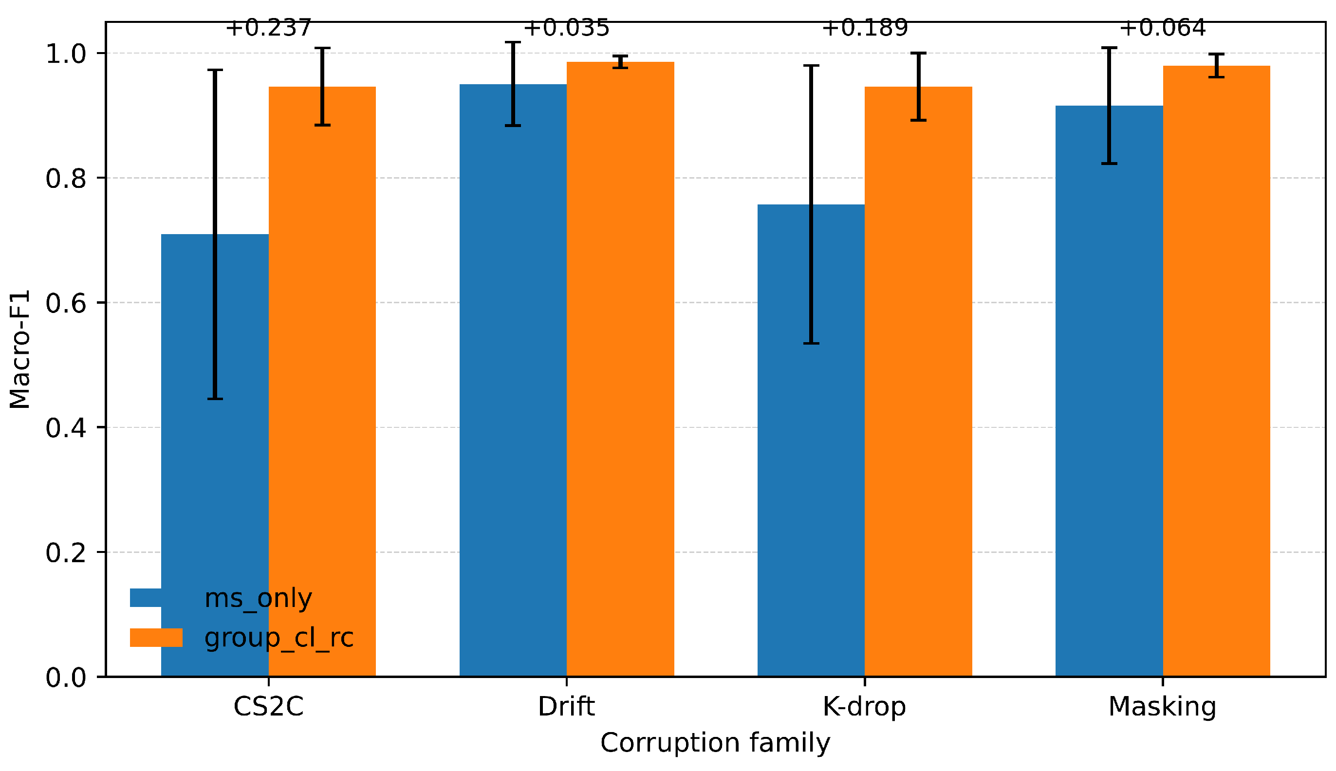
Masking	0.9159 ± 0.0929	0.9797 ± 0.0185	+0.0638 ± 0.0846	320

reports the full-grid matched averages, and Figure 2 provides the corresponding visual summary.

Group-CL-RC improves Macro-F1 over ms_only across all four corruption families. The largest gains occur under CS2C, where Macro-F1 increases from 0.7094 to 0.9465, and under K-drop, where it increases from 0.7572 to 0.9461. These families directly disrupt non-visible spectral information and are therefore central to evaluating relation-aware multispectral robustness. The CS2C result should be interpreted within the controlled matched perturbation protocol used here: it demonstrates strong stability under the defined compound stress test, but not a universal guarantee against all real-world spectral–spatial shifts.

Drift and masking produce smaller but consistently positive gains, with Macro-F1 increasing from 0.9506 to 0.9860 under drift and from 0.9159 to 0.9797 under masking. Because the K-drop grid contains a target-dependent number of perturbation levels, a target-balanced family average was also computed; the K-drop gain remains substantial at +0.1688 Macro-F1.

Table 5. Backbone-wise matched robustness comparison between ms_only and Group-CL-RC on EuroSAT. Results report Macro-F1 mean ± standard deviation over matched evaluation points. For each backbone, the higher mean Macro-F1 value between the two methods is highlighted in bold.

Corruption	Backbone	ms_only	Group-CL-RC	$\mathbf{\Delta }$
CS2C	ConvNeXt-Tiny	0.7178 ± 0.2619	0.9574 ± 0.0502	+0.2396 ± 0.2267
CS2C	EfficientNet-B0	0.7363 ± 0.2456	0.9560 ± 0.0437	+0.2198 ± 0.2083
CS2C	ResNet-50	0.6873 ± 0.2883	0.9610 ± 0.0373	+0.2737 ± 0.2596
CS2C	Swin-Tiny	0.6961 ± 0.2601	0.9115 ± 0.0885	+0.2154 ± 0.1943
Drift	ConvNeXt-Tiny	0.9676 ± 0.0364	0.9899 ± 0.0018	+0.0223 ± 0.0357
Drift	EfficientNet-B0	0.9444 ± 0.0734	0.9851 ± 0.0088	+0.0407 ± 0.0663
Drift	ResNet-50	0.9277 ± 0.0939	0.9862 ± 0.0041	+0.0585 ± 0.0923
Drift	Swin-Tiny	0.9625 ± 0.0376	0.9825 ± 0.0154	+0.0201 ± 0.0295
K-drop	ConvNeXt-Tiny	0.7657 ± 0.2212	0.9611 ± 0.0380	+0.1954 ± 0.1903
K-drop	EfficientNet-B0	0.8195 ± 0.1819	0.9563 ± 0.0413	+0.1367 ± 0.1455
K-drop	ResNet-50	0.7617 ± 0.2144	0.9508 ± 0.0402	+0.1891 ± 0.1814
K-drop	Swin-Tiny	0.6818 ± 0.2497	0.9164 ± 0.0753	+0.2347 ± 0.1886
Masking	ConvNeXt-Tiny	0.9328 ± 0.0742	0.9833 ± 0.0137	+0.0505 ± 0.0631
Masking	EfficientNet-B0	0.9312 ± 0.0604	0.9815 ± 0.0195	+0.0503 ± 0.0531
Masking	ResNet-50	0.8747 ± 0.1358	0.9827 ± 0.0107	+0.1080 ± 0.1289
Masking	Swin-Tiny	0.9247 ± 0.0702	0.9712 ± 0.0246	+0.0465 ± 0.0535

decomposes the matched robustness comparison by backbone. Group-CL-RC improves over ms_only for all four backbones and all corruption families, showing that the robustness gain is not restricted to a single architecture.

Under CS2C, gains remain large across architectures, ranging from +0.2154 on Swin-Tiny to +0.2737 on ResNet-50. Under K-drop, gains range from +0.1367 on EfficientNet-B0 to +0.2347 on Swin-Tiny, supporting the conclusion that Group-CL-RC is especially useful when spectral-group availability is disrupted. Drift produces smaller but positive gains, while masking yields intermediate improvements. Target-wise results in Supplementary Section S1.6 and Supplementary Figure S1 further show positive gains for all evaluated spectral targets.

5.3. Statistical Significance of EuroSAT Robustness Gains

We next assess whether the robustness gains observed on EuroSAT are statistically supported under matched evaluation. The analysis is performed on paired Macro-F1 values, where each pair compares ms_only and Group-CL-RC under the same backbone, checkpoint seed, corruption family, target group, and perturbation level.

To avoid diluting robustness effects with unperturbed or near-clean levels, the main statistical table focuses on non-clean perturbation conditions. These results are summarizes in

Table 6. Paired statistical analysis of EuroSAT robustness gains under non-clean perturbation conditions. Results compare Group-CL-RC against ms_only using matched Macro-F1 pairs. Holm-corrected paired t-test and Wilcoxon p-values are reported.

Test Set	n	ms_only	Group-CL-RC	Gain	Rel. Gain	Holm ${\mathit{p}}_{\mathit{t}}$	Holm ${\mathit{p}}_{\mathit{w}}$
Global	1000	0.7807	0.9560	+0.1753	+22.46%	$2.31\times {10}^{-144}$	$1.66\times {10}^{-164}$
CS2C	240	0.6165	0.9323	+0.3158	+51.23%	$8.47\times {10}^{-65}$	$1.20\times {10}^{-40}$
Drift	240	0.9381	0.9849	+0.0468	+4.99%	$1.76\times {10}^{-21}$	$1.20\times {10}^{-40}$
K-drop	280	0.6912	0.9339	+0.2427	+35.11%	$4.15\times {10}^{-69}$	$4.55\times {10}^{-47}$
Masking	240	0.8918	0.9766	+0.0847	+9.50%	$1.62\times {10}^{-35}$	$1.20\times {10}^{-40}$

. Full-grid statistical results, including all perturbation levels, are reported in Supplementary Section S1.3 and Supplementary Table S13.

The paired analysis confirms that the EuroSAT robustness gains are statistically supported. Across all non-clean perturbation conditions, Group-CL-RC improves Macro-F1 from 0.7807 to 0.9560, corresponding to a +0.1753 absolute gain and a +22.46% relative improvement. This global improvement remains significant after Holm correction for both the paired t-test and the Wilcoxon signed-rank test.

Family-wise results show the largest supported gains under CS2C and K-drop, followed by masking and drift. Thus, the improvements reported in Table 4 reflect systematic matched gains rather than isolated numerical fluctuations. For completeness, the clean paired comparison also shows a small supported Macro-F1 gain, from 0.9879 to 0.9890 over 20 matched clean pairs; its magnitude confirms that the main contribution of Group-CL-RC lies in robustness rather than nominal clean accuracy.

5.4. Matched External-Baseline Comparison

To address the need for a direct quantitative comparison with representative external learning objectives, we add a matched EuroSAT All Bands comparison. Rather than comparing with published scores obtained under different modalities, band configurations, splits, or robustness protocols, all baselines are implemented within the same pipeline and evaluated with the same train/test split, three seeds, checkpoint-selection criterion, compact robustness grid, and Macro-F1 metric.

The comparison includes three representative baselines. CorruptTrain-MS is our controlled supervised corruption-augmentation baseline: each sample is optimized with the same classification objective using clean and structured-corrupted multispectral views, following the general corruption-robustness and image-augmentation paradigms [5,23]. Because no named published architecture is reproduced, CorruptTrain-MS should be interpreted as an implementation-controlled baseline rather than as a direct reimplementation of a specific published method. SupCon-MS adapts the supervised contrastive loss of Khosla et al. [32] to the fused multispectral representation. Paired-View InfoNCE-MS adapts the SimCLR contrastive formulation of Chen et al. [29], treating the clean and structured-corrupted multispectral views of the same image as the positive pair. Group-CL-RC is evaluated with the default VIS–NIR–SWIR descriptor for both ConvNeXt-Tiny and Swin-Tiny; the red-edge-aware descriptor is kept as a separate descriptor-granularity ablation. This block is interpreted descriptively rather than as a separate inferential dominance test. Additional family-level results for the matched external-baseline comparison are reported in the Supplementary Materials, where ConvNeXt-Tiny and Swin-Tiny are detailed separately.

Table 7. Matched external-baseline comparison on EuroSAT All Bands using ConvNeXt-Tiny and Swin-Tiny. Results report Macro-F1 mean ± standard deviation over three seeds. Robust Avg. is computed as the mean over the non-clean compact robustness families. Family-level details are provided in the Supplementary Materials.

Backbone	Method	Clean	Robust Avg.
ConvNeXt-Tiny	Group-CL-RC	$0.9868\pm 0.0006$	$0.9687\pm 0.0082$
ConvNeXt-Tiny	CorruptTrain-MS	$0.9858\pm 0.0019$	$0.9751\pm 0.0031$
ConvNeXt-Tiny	SupCon-MS	$0.9874\pm 0.0027$	$0.9513\pm 0.0054$
ConvNeXt-Tiny	Paired-View InfoNCE-MS	$0.9853\pm 0.0019$	$0.9653\pm 0.0037$
Swin-Tiny	Group-CL-RC	$0.9876\pm 0.0010$	$0.9195\pm 0.0252$
Swin-Tiny	CorruptTrain-MS	$0.9836\pm 0.0011$	$0.9728\pm 0.0007$
Swin-Tiny	SupCon-MS	$0.9861\pm 0.0012$	$0.9151\pm 0.0159$
Swin-Tiny	Paired-View InfoNCE-MS	$0.9841\pm 0.0013$	$0.9611\pm 0.0089$

shows that the matched external baselines are strong competitors. On ConvNeXt-Tiny, Group-CL-RC remains close to the strongest robust average and outperforms the two contrastive baselines in aggregate robustness. CorruptTrain-MS obtains the highest robust average, confirming that direct supervised exposure to structured corruptions is a strong robustness factor.

On Swin-Tiny, CorruptTrain-MS is clearly stronger under the compact robustness protocol, while Group-CL-RC preserves the highest clean Macro-F1 among the compared methods. These results position Group-CL-RC as a competitive and interpretable spectral-relation objective, not as a universally dominant replacement for corruption-training strategies. They also clarify that robustness behavior is architecture-dependent under structured multispectral degradation.

5.5. External Validation on SEN12MS

We further evaluate Group-CL-RC on SEN12MS as an external Sentinel-2-only validation setting. As described in Section 4.1, the Sentinel-1 component is excluded, and the evaluation is restricted to the ten retained Sentinel-2 bands used in our SEN12MS setting. This 10-band input retains the VIS, NIR, and SWIR bands required by the relation-consistency descriptor, which keeps the protocol aligned with the proposed VIS–NIR–SWIR framework. The goal is not to establish benchmark-leading SEN12MS performance, but to assess whether the EuroSAT robustness trends remain meaningful under different scenes, class distributions, spatial coverage, and seasonal conditions.

Table 8. External validation on SEN12MS using the Sentinel-2 component only. Results report Macro-F1 mean ± standard deviation over the strictly aligned validation grid. Clean uses 12 scores per variant. Drift uses severity 2 and is averaged over 36 non-clean scores per variant. K-drop and CS2C use severities 2 and 3 and are each averaged over 72 non-clean scores per variant. Robust Avg. is the unweighted average of the three family-level means and is reported as a compact aggregate. For each protocol–backbone setting and evaluation column, the highest mean Macro-F1 value among the compared variants is highlighted in bold.

Variant	Clean	Drift	K-Drop	CS2C	Robust Avg.
ms_only	0.6036 ± 0.0286	0.5223 ± 0.0294	0.4324 ± 0.0551	0.2288 ± 0.0618	0.3945
group_cl	0.5876 ± 0.0363	0.5609 ± 0.0238	0.5128 ± 0.0349	0.4278 ± 0.0616	0.5005
Group-CL-RC	0.5907 ± 0.0356	0.5541 ± 0.0221	0.5333 ± 0.0325	0.4117 ± 0.0610	0.4997

reports the compact SEN12MS summary. Clean performance is averaged over two protocols, two backbones, and three seeds. The robustness columns report Macro-F1 over the strictly aligned non-clean validation grid: drift uses severity 2, while K-drop and CS2C use severities 2 and 3. Robust Avg. is the unweighted average of the three family-level means and is used only as a compact aggregate.

The SEN12MS results are more challenging than the EuroSAT results, as expected for an external validation setting with different sampling, taxonomy, geographic coverage, and seasonal structure. On clean SEN12MS samples, ms_only obtains the highest Macro-F1, so the external validation does not indicate a clean-performance advantage for Group-CL-RC. This is consistent with the role of Group-CL-RC as a robustness-oriented regularizer rather than a mechanism primarily designed to improve nominal accuracy.

Under non-clean perturbations, both group-structured variants substantially improve over ms_only. Group-CL-RC increases the robust average from 0.3945 to 0.4997, while group_cl obtains a similar value of 0.5005. The paired analysis shows that Group-CL-RC significantly improves over ms_only at the pooled non-clean level, but is not globally different from group_cl. Thus, SEN12MS supports the robustness value of group-structured learning while limiting any claim of universal Group-CL-RC superiority over standard Group-CL.

The clearest Group-CL-RC-specific advantage appears under K-drop. Group-CL-RC reaches 0.5333 Macro-F1, compared with 0.4324 for ms_only and 0.5128 for group_cl; the gain over group_cl remains statistically supported after Holm correction. Under CS2C, both group-structured variants remain well above ms_only, but group_cl obtains the higher mean. Overall, SEN12MS strengthens the paper in a controlled and conservative way: the EuroSAT robustness conclusions are not confined to a single dataset, but the added benefit of relation consistency remains perturbation-dependent.

5.6. Objective-Component Ablation

We next isolate the contributions of group-level contrastive alignment and relation consistency by comparing group_cl, group_rc, and Group-CL-RC. The ablation is evaluated with ConvNeXt-Tiny and Swin-Tiny over three seeds.

Table 9. Global objective-component ablation under four corruption families. Results report mean Macro-F1 over ConvNeXt-Tiny and Swin-Tiny using three seeds. ${\Delta }_{\mathrm{RC}}$ denotes the gain of group_rc over group_cl. ${\Delta }_{\mathrm{syn}}$ denotes the gain of Group-CL-RC over the best single-component variant. For each corruption family, the highest mean Macro-F1 value among the compared variants is highlighted in bold.

Corruption	group_cl	group_rc	Group-CL-RC	${\mathbf{\Delta }}_{\mathbf{RC}}$	${\mathbf{\Delta }}_{\mathbf{syn}}$
CS2C	0.8082	0.9289	0.9205	+0.1207	−0.0084
Drift	0.9838	0.9858	0.9871	+0.0020	+0.0013
K-drop	0.8832	0.8813	0.9302	−0.0019	+0.0470
Masking	0.9418	0.9770	0.9639	+0.0352	−0.0131

reports the global results across the four corruption families.

The ablation reveals a perturbation-dependent profile. Relation consistency is not merely a secondary add-on to Group-CL: group_rc is itself a strong robustness mechanism, especially under CS2C and masking. Under CS2C, group_rc improves over group_cl by +0.1207 Macro-F1 and obtains the highest global mean; under masking, it also obtains the best mean, with a +0.0352 gain over group_cl.

Under K-drop, the full Group-CL-RC objective performs best, improving over the best single-component variant by +0.0470. This indicates that group-level contrastive alignment and relation consistency are most complementary when spectral-group availability is directly degraded. The backbone-wise analysis in Supplementary Section S1.9 and Supplementary Table S19 supports the same interpretation: Group-CL-RC is best under K-drop for both ConvNeXt-Tiny and Swin-Tiny, whereas the best variant under CS2C and masking depends on the corruption family and backbone.

5.7. Descriptor-Granularity Ablation

We further test whether a finer relation descriptor improves EuroSAT robustness. This descriptor-granularity ablation uses ConvNeXt-Tiny over three seeds. The default Group-CL-RC descriptor models the three pairwise VIS–NIR–SWIR relations, whereas the red-edge-aware descriptor adds the Sentinel-2 red-edge bands as a fourth group, increasing the descriptor size from three to six pairwise relations. The results of this ablation are reported in

Table 10. Descriptor-granularity ablation for Group-CL-RC on EuroSAT using ConvNeXt-Tiny. Results report mean Macro-F1 over three seeds. Robust Avg. denotes the mean over the non-clean EuroSAT descriptor-ablation evaluation points. Training time reports total wall-clock training time. For each performance metric, the highest mean Macro-F1 value is highlighted in bold, whereas for training time, the lowest value is highlighted in bold.

Descriptor	Dim.	Clean	Robust Avg.	Drift	K-Drop	CS2C	Training Time (h)
Default VIS–NIR–SWIR	3	0.9868 ± 0.0006	0.9571 ± 0.0408	0.9845 ± 0.0019	0.9759 ± 0.0105	0.9340 ± 0.0472	2.531 ± 0.007
Red-edge-aware	6	0.9887 ± 0.0015	0.9680 ± 0.0316	0.9859 ± 0.0029	0.9811 ± 0.0076	0.9524 ± 0.0389	3.025 ± 0.007

.

The red-edge-aware descriptor improves the global non-clean Macro-F1 from 0.9571 to 0.9680, a +0.0109 absolute gain. This robustness gain remains statistically supported after Holm correction, whereas the smaller clean Macro-F1 increase is not statistically significant. At the family level, the largest numerical gain occurs under CS2C, suggesting that explicitly separating red-edge bands can help when spectral and spatial degradations jointly affect the multispectral input.

This improvement comes with a measurable cost: the descriptor size increases from three to six relations, and average training time rises from 2.531 h to 3.025 h, an overhead of approximately +19.5%. We therefore retain the compact VIS–NIR–SWIR descriptor as the default configuration, while treating the red-edge-aware descriptor as a more robust but more expensive alternative.

5.8. Training-Time Corruption Ablation

We next analyze how the training-time corruption used to construct the degraded view affects Group-CL-RC. This ablation is conducted on EuroSAT with ConvNeXt-Tiny over three seeds. We compare K-drop on NIR + SWIR bands, drift on non-RGB bands, masking on non-RGB bands, and a mixed strategy that samples heterogeneous corruption types. All variants are evaluated on the same clean and robustness grid.

The training-time corruption ablation results are reported in

Table 11. Training-time corruption ablation for Group-CL-RC on EuroSAT using ConvNeXt-Tiny. Results report mean Macro-F1 over three seeds. Robust Avg. denotes the mean over the non-clean evaluation conditions. For each evaluation column, the highest mean Macro-F1 value among the compared training-time corruption settings is highlighted in bold.

Training Corruption	Clean	Robust Avg.	Drift	Masking	K-Drop	CS2C
K-drop NIR + SWIR	0.9885 ± 0.0005	0.9700± 0.0022	0.9876± 0.0009	0.9764 ± 0.0012	0.9820± 0.0032	0.9491 ± 0.0047
Drift non-RGB bands	0.9884 ± 0.0008	0.9632 ± 0.0099	0.9868 ± 0.0006	0.9764 ± 0.0062	0.9614 ± 0.0054	0.9417 ± 0.0214
Masking non-RGB bands	0.9887± 0.0004	0.9693 ± 0.0016	0.9874 ± 0.0004	0.9856± 0.0011	0.9523 ± 0.0147	0.9576± 0.0056
Mixed	0.9878 ± 0.0016	0.9629 ± 0.0103	0.9870 ± 0.0017	0.9837 ± 0.0019	0.9755 ± 0.0054	0.9302 ± 0.0229

.

All four training-time corruption strategies preserve similar clean Macro-F1, with differences below 0.001. Thus, the corruption choice mainly affects robustness rather than nominal clean performance. K-drop on NIR + SWIR bands obtains the highest aggregate robustness and the best K-drop performance, supporting its use as the default training-time corruption for Group-CL-RC.

The best training corruption nevertheless depends on the evaluation family. Masking non-RGB bands performs best under masking and also obtains the highest CS2C Macro-F1, indicating that spatially structured degradation during training can help when evaluation includes masking or compound spectral–spatial effects. However, it is weaker under K-drop than K-drop NIR + SWIR training. The mixed strategy does not dominate the structured single-corruption strategies, suggesting that heterogeneous corruption exposure alone is not sufficient to improve global robustness.

5.9. Worst-Case and Retention Analysis

The previous sections report average robustness gains. We now examine whether the benefit of relation consistency also appears under severe perturbations and observed worst-case diagnostic points. This analysis compares group_cl with Group-CL-RC to isolate the effect of adding relation consistency on top of group-level contrastive learning.

Table 12. Worst-case robustness comparison between group_cl and Group-CL-RC. The table reports the lowest observed Macro-F1 over non-clean diagnostic points for each corruption family. For each corruption family, the higher worst-case Macro-F1 value between the two methods is highlighted in bold.

Corruption	group_cl	Group-CL-RC	Gain
CS2C	0.5749	0.7409	+0.1660
Drift	0.9348	0.9751	+0.0404
K-drop	0.6226	0.7065	+0.0839
Masking	0.8382	0.8702	+0.0319

shows that Group-CL-RC improves the observed worst-case Macro-F1 over group_cl in all four corruption families. The largest gain occurs under CS2C, where worst-case Macro-F1 increases from 0.5749 to 0.7409, followed by K-drop, where it increases from 0.6226 to 0.7065.

Table 13. Robustness retention of group_cl and Group-CL-RC. Retention measures the fraction of clean Macro-F1 preserved under non-clean diagnostic perturbations. For each corruption family, the higher retention value between the two methods is highlighted in bold.

Corruption	Variant	F1 Retention	Worst F1 Retention	F1 Drop
CS2C	group_cl	0.7573 ± 0.1176	0.5812	0.2398 ± 0.1161
CS2C	Group-CL-RC	0.9076 ± 0.0753	0.7494	0.0914 ± 0.0745
Drift	group_cl	0.9904 ± 0.0141	0.9427	0.0095 ± 0.0140
Drift	Group-CL-RC	0.9974 ± 0.0039	0.9882	0.0026 ± 0.0039
K-drop	group_cl	0.8673 ± 0.1010	0.6313	0.1310 ± 0.0996
K-drop	Group-CL-RC	0.9256 ± 0.0733	0.7146	0.0735 ± 0.0724
Masking	group_cl	0.9340 ± 0.0471	0.8463	0.0654 ± 0.0466
Masking	Group-CL-RC	0.9661 ± 0.0313	0.8818	0.0335 ± 0.0309

confirms the worst-case findings through a retention-based analysis. Across all corruption families, Group-CL-RC preserves a larger fraction of clean Macro-F1 than group_cl. The improvement is particularly visible under CS2C, where mean F1 retention increases from 0.7573 to 0.9076 and worst-case retention increases from 0.5812 to 0.7494. Under K-drop, mean retention increases from 0.8673 to 0.9256 and worst-case retention increases from 0.6313 to 0.7146. Masking and drift also show improved retention, although their absolute F1 drops are smaller.

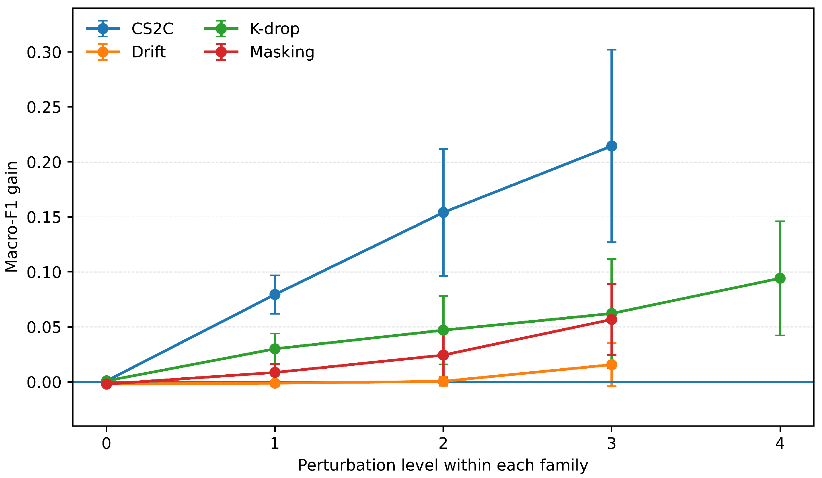
Figure 3 summarizes the severity-level gains. Because perturbation levels have family-specific meanings, the x-axis should be read as an ordinal severity index within each corruption family. At clean or near-clean levels, differences between group_cl and Group-CL-RC are negligible and can be slightly negative. As perturbations become more severe, relation consistency provides larger gains, especially under CS2C, K-drop on NIR + SWIR, and masking. The full severity-level diagnostic table is provided in Supplementary Section S1.5 and Supplementary Table S17.

5.10. Relation-Deformation Sensitivity Analysis

We finally analyze the relationship between relation deformation and classification degradation. This diagnostic clarifies the role of the relation-consistency regularizer and avoids interpreting $D_{\mathrm{RC}}$ as a direct performance metric. Here, $D_{\mathrm{RC}}$ measures perturbation-induced deformation in the inter-group relation descriptor, whereas Macro-F1 drop measures downstream degradation relative to the corresponding clean condition. A model may therefore exhibit larger raw relation deformation while remaining less sensitive to that deformation at the decision level.

Table 14. Global relation-deformation sensitivity analysis. $D_{\mathrm{RC}}$ denotes relation deformation. Mean F1 Drop denotes the average decrease in Macro-F1 relative to the corresponding clean condition across the non-clean diagnostic points. The slope quantifies the decision-level sensitivity of Macro-F1 degradation to relation deformation. Lower values of both Mean F1 Drop and slope indicate greater robustness, and the lowest value for each metric among the compared variants is highlighted in bold.

Variant	n	Pearson r	Slope	Mean ${\mathit{D}}_{\mathbf{RC}}$	Mean F1 Drop
group_cl	150	0.6806	0.2623	0.2705	0.0767
Group-CL-RC	150	0.6990	0.0917	0.7219	0.0357

reports the global sensitivity of Macro-F1 degradation to relation deformation. Compared with group_cl, Group-CL-RC substantially reduces the slope between $D_{\mathrm{RC}}$ and Macro-F1 drop, from 0.2623 to 0.0917, while also reducing the mean Macro-F1 drop from 0.0767 to 0.0357. This occurs even though the mean raw $D_{\mathrm{RC}}$ is higher for Group-CL-RC. The result supports the interpretation that relation consistency primarily reduces decision-level sensitivity to relation deformation rather than uniformly minimizing deformation magnitude.

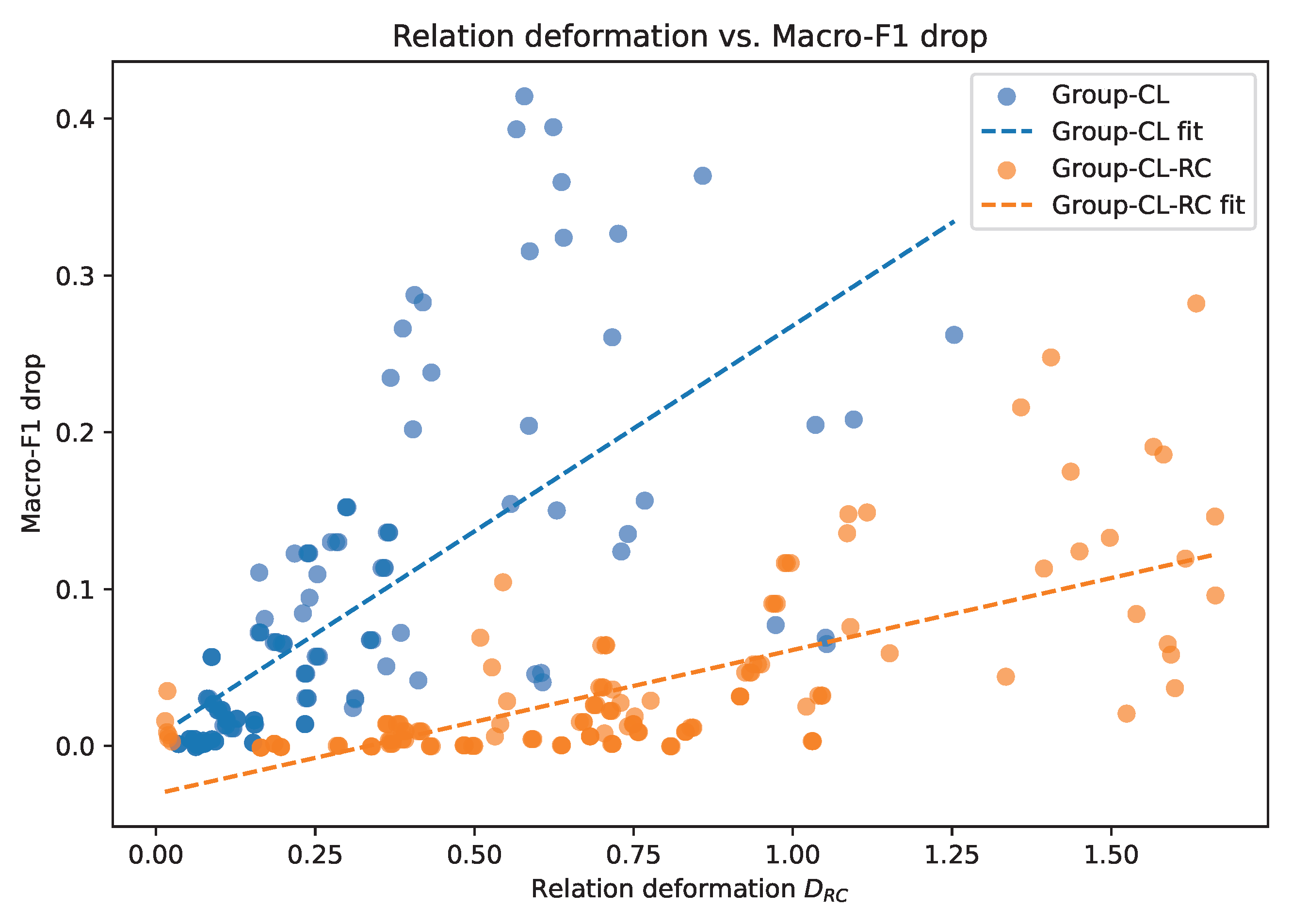
Figure 4 visually supports the conclusion drawn from Table 14. The Group-CL-RC points can occupy higher $D_{\mathrm{RC}}$ ranges, but their associated Macro-F1 drops remain lower on average. This supports the interpretation that the relation-consistency objective improves tolerance to relation deformation, rather than uniformly suppressing the deformation magnitude itself.

The family-wise analysis in

Table 15. Family-wise relation-deformation sensitivity analysis. $D_{\mathrm{RC}}$ denotes relation deformation, and Mean F1 Drop denotes the average decrease in Macro-F1 relative to the corresponding clean condition within each corruption family. The slope quantifies the sensitivity of Macro-F1 degradation to relation deformation. Lower slope and lower Mean F1 Drop indicate greater decision-level robustness. For each corruption family, the lowest slope and Mean F1 Drop values among the compared variants are highlighted in bold.

Corruption	Variant	n	Slope ${\mathit{D}}_{\mathbf{RC}}\to$ F1 Drop	Mean ${\mathit{D}}_{\mathbf{RC}}$	Mean F1 Drop
CS2C	group_cl	18	0.6524	0.4069	0.2398
CS2C	Group-CL-RC	18	0.2026	1.0752	0.0914
Drift	group_cl	54	0.0665	0.0964	0.0095
Drift	Group-CL-RC	54	0.0092	0.5471	0.0026
K-drop	group_cl	24	0.1816	0.6948	0.1310
K-drop	Group-CL-RC	24	0.0685	0.9329	0.0735
Masking	group_cl	54	0.3943	0.2105	0.0654
Masking	Group-CL-RC	54	0.0891	0.6850	0.0335

supports the same interpretation. The slope is lower for Group-CL-RC in all four corruption families, with the clearest reductions under CS2C, K-drop, and masking. Drift should be interpreted more cautiously because absolute F1 drops remain small for both variants.

The bucket analysis further illustrates this tolerance effect. Across low, mid, and high relation-deformation regimes, Group-CL-RC produces lower Macro-F1 drops than group_cl. Thus, even when the relation descriptor is substantially affected by perturbation, Group-CL-RC tends to preserve the final classification decision more effectively.

Additional point-level and family-wise diagnostics are reported in Supplementary Section S1.7, Supplementary Table S18, and Supplementary Figures S2–S5. These supplementary results include the detailed relation-deformation values, Macro-F1 drops, deformation-normalized drops, family-specific sensitivity summaries, and family-wise scatter plots used to support the interpretation in Table 14, Table 15 and

Table 16. Bucket-level analysis of Macro-F1 drop across relation-deformation regimes. Negative values of $\Delta$ indicate a lower F1 drop for Group-CL-RC relative to group_cl. Within each relation-deformation bucket, the lower mean F1 drop between the two variants is highlighted in bold.

${\mathit{D}}_{\mathbf{RC}}$ Bucket	group_cl F1 Drop	Group-CL-RC F1 Drop	$\mathbf{\Delta }$
Low	0.0225	0.0049	−0.0176
Mid	0.1350	0.0095	−0.1255
High	0.1982	0.0555	−0.1427

and Figure 4.

Overall, the relation-deformation diagnostics show that relation consistency acts as a tolerance-inducing regularizer. It does not simply force relation descriptors to remain close under every corruption. Instead, it shapes the representation so that perturbation-induced changes in inter-group relations have a smaller effect on the final decision. Together with the robustness, ablation, worst-case, and retention analyses, this supports inter-group relational geometry as an interpretable robustness target for multispectral classification.

5.11. Qualitative Analysis

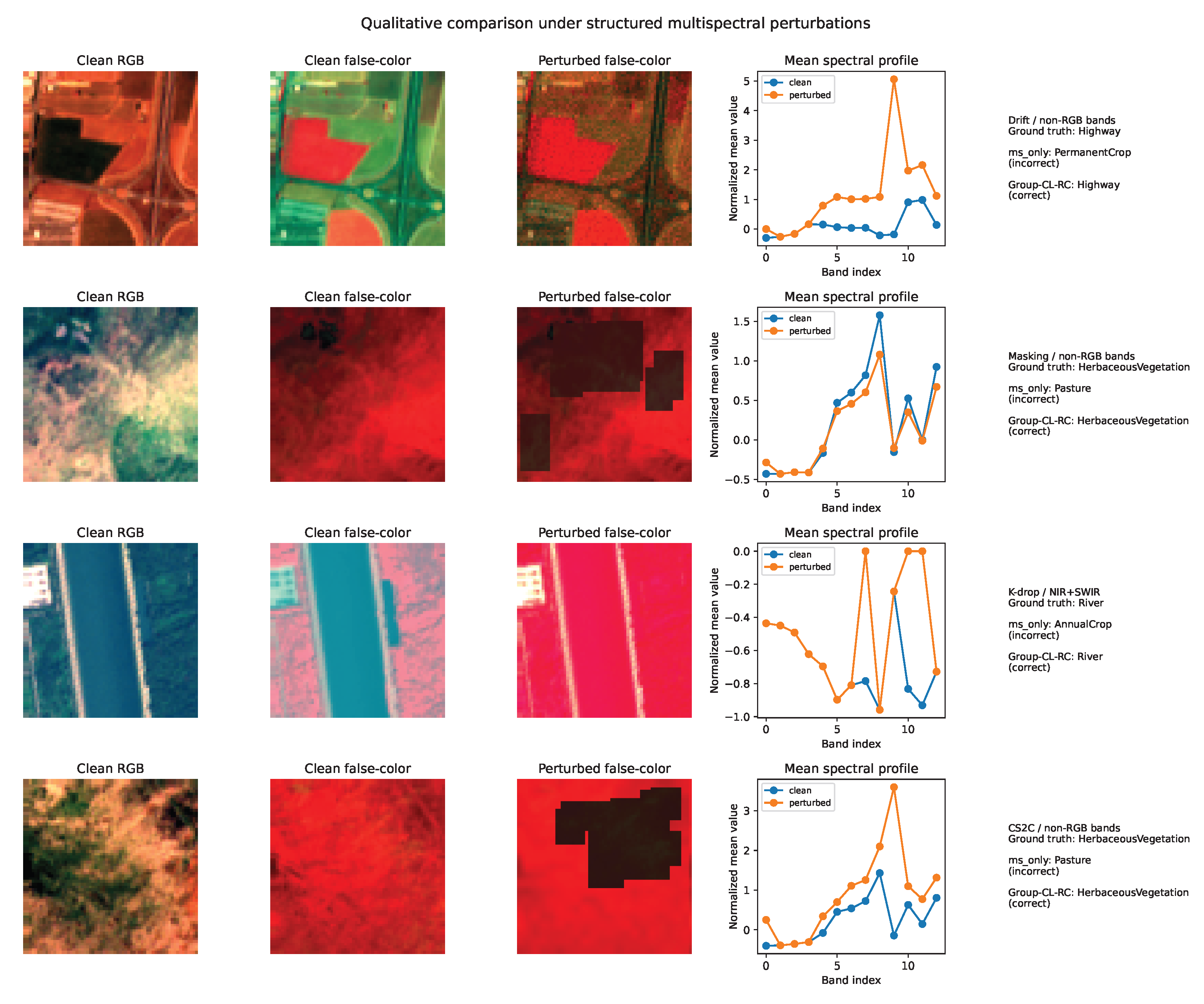
To complement the quantitative robustness results, Figure 5 provides representative qualitative examples. The selected cases illustrate situations where the multispectral-only baseline changes to an incorrect prediction under structured perturbation, whereas Group-CL-RC preserves the correct class decision. These examples are illustrative rather than statistical evidence, and should be read together with the matched robustness, ablation, retention, and relation-deformation analyses.

In the drift example, the true class is Highway. The baseline changes from Highway under the clean input to PermanentCrop under drift on non-RGB bands, whereas Group-CL-RC preserves the Highway prediction. The masking and CS2C examples involve HerbaceousVegetation samples for which the baseline changes to Pasture, while Group-CL-RC preserves the correct class. The K-drop example corresponds to a River sample under NIR + SWIR band removal; the baseline changes to AnnualCrop, whereas Group-CL-RC preserves River.

Overall, the qualitative examples provide concrete illustrations of the robustness behavior quantified above. They should not be interpreted as additional statistical proof; the main evidence remains the matched quantitative evaluation, statistical tests, ablations, and diagnostic analyses.

5.12. Computational Profiling

We finally report computational profiling results for the main model variants. This analysis is included to clarify the practical cost of the proposed objective and to distinguish training-time overhead from inference-time model complexity. Profiling is conducted on EuroSAT using ConvNeXt-Tiny and Swin-Tiny over three seeds. For each backbone, we compare ms_only, group_cl, group_rc, and Group-CL-RC. The profiling runs use six training epochs and report average wall-clock time per epoch, training throughput, peak GPU memory, trainable parameters, and forward-pass MACs.

Table 17. Computational profiling of the main model variants on EuroSAT. The table reports trainable parameters, THOP forward-pass MACs, average wall-clock time per epoch, training throughput, and peak GPU memory over three profiling seeds. Time overhead is measured relative to ms_only for the same backbone.

Backbone	Variant	Params (M)	MACs (G)	Time/Epoch (s)	Time Ratio	Throughput (img/s)	Peak GPU (MB)
ConvNeXt-Tiny	ms_only	56.57 ± 0.00	1.84 ± 0.00	53.28 ± 0.42	1.00×	362.59 ± 2.89	2332.00 ± 0.00
ConvNeXt-Tiny	group_cl	56.57 ± 0.00	1.84 ± 0.00	70.97 ± 0.32	1.33×	272.17 ± 1.22	1824.67 ± 1.15
ConvNeXt-Tiny	group_rc	56.57 ± 0.00	1.84 ± 0.00	106.92 ± 0.42	2.01×	180.67 ± 0.71	3038.67 ± 1.15
ConvNeXt-Tiny	Group-CL-RC	56.57 ± 0.00	1.84 ± 0.00	108.00 ± 0.88	2.03×	178.86 ± 1.47	2602.00 ± 0.00
Swin-Tiny	ms_only	55.94 ± 0.00	2.07 ± 0.00	89.30 ± 0.15	1.00×	216.32 ± 0.35	2956.00 ± 0.00
Swin-Tiny	group_cl	55.94 ± 0.00	2.07 ± 0.00	126.34 ± 0.61	1.41×	152.90 ± 0.74	2260.00 ± 0.00
Swin-Tiny	group_rc	55.94 ± 0.00	2.07 ± 0.00	203.20 ± 0.80	2.28×	95.06 ± 0.37	3970.00 ± 0.00
Swin-Tiny	Group-CL-RC	55.94 ± 0.00	2.07 ± 0.00	204.89 ± 0.27	2.29×	94.28 ± 0.12	3444.00 ± 0.00

shows that, for a fixed backbone, trainable parameters and forward-pass MACs remain essentially unchanged across variants. This is expected because the inference-time decision pathway is shared, whereas the auxiliary group-level and relation-consistency objectives are used only during training. Thus, Group-CL-RC does not introduce a substantially heavier inference architecture.

The main cost appears during training. For ConvNeXt-Tiny, the average time per epoch increases from 53.28 s for ms_only to 108.00 s for Group-CL-RC, corresponding to a 2.03× overhead. For Swin-Tiny, it increases from 89.30 s to 204.89 s, corresponding to a 2.29× overhead. This overhead is mainly due to degraded-view processing and relation-consistency computation.

Peak GPU memory remains within a practical range in the evaluated setting. For Group-CL-RC, measured peak memory is 2602 MB with ConvNeXt-Tiny and 3444 MB with Swin-Tiny. Overall, Group-CL-RC introduces a real but training-focused overhead while keeping inference complexity essentially unchanged. This trade-off is consistent with the design of the method: relation consistency improves robustness through auxiliary training constraints rather than through a substantially larger inference model.

6. Discussion

6.1. Main Findings

The experimental results support the central premise of this work: inter-group relational geometry is a meaningful target for improving robustness in multispectral remote sensing classification. Across EuroSAT clean, robustness, ablation, and diagnostic settings, Group-CL-RC preserves strong nominal performance while improving robustness under structured spectral and spectral–spatial degradation. The largest gains occur under CS2C and K-drop, indicating that the method is most useful when non-visible spectral information and cross-spectral complementarity are directly disrupted.

The matched external-baseline comparison places these gains in a more conservative context. CorruptTrain-MS is a strong supervised corruption-training baseline, especially with Swin-Tiny, whereas Group-CL-RC remains competitive and preserves an explicit spectral-relation objective. Thus, the contribution should be interpreted as a relation-aware robustness mechanism rather than as a universally dominant replacement for all corruption-training strategies.

The SEN12MS validation further supports this interpretation. Group-structured learning improves robustness over the multispectral-only baseline under the constructed Sentinel-2-only protocols, but the advantage of Group-CL-RC over standard Group-CL remains perturbation-dependent. The objective-component ablation clarifies this behavior: relation consistency is an effective robustness mechanism in its own right, while its combination with Group-CL is most clearly justified when spectral-group availability is degraded.

6.2. Interpretation of Relation Consistency

The relation-consistency term regularizes the internal similarity structure among VIS, NIR, and SWIR group embeddings across clean and corrupted views. However, it should not be interpreted as enforcing strict invariance of the relation descriptor under every corruption. Some perturbations can legitimately alter inter-group relations, especially when non-visible spectral groups are removed, masked, or strongly distorted.

The relation-deformation sensitivity analysis provides a more precise interpretation. Group-CL-RC does not uniformly reduce the raw magnitude of relation deformation measured by $D_{\mathrm{RC}}$. Instead, it reduces the downstream sensitivity of the classifier to perturbation-induced relation changes. The model can therefore experience measurable descriptor deformation while preserving a more stable classification decision.

This tolerance-based interpretation is important. The goal is not to make all clean and corrupted relation descriptors identical, but to learn representations in which inter-group spectral relations remain useful and less fragile for the final decision. The worst-case, retention, bucket-level, and relation-deformation diagnostics consistently support this interpretation.

6.3. Clean Accuracy and Robustness Are Distinct Objectives

The clean evaluation confirms that high nominal performance does not fully characterize multispectral model reliability. Several variants achieve strong clean Macro-F1, and differences among competitive multispectral models remain small under clean conditions. However, the robustness evaluation reveals substantially different behaviors when inputs are affected by structured spectral and spectral–spatial degradation.

This distinction is central for multispectral remote sensing. A model evaluated only under clean conditions may appear reliable while remaining vulnerable to degradation of NIR or SWIR information. Such degradation is practically important because non-visible bands provide vegetation, moisture, and material-composition cues that cannot be fully recovered from RGB channels alone. The gains obtained by Group-CL-RC, especially under CS2C and K-drop, therefore support treating robustness as a primary evaluation axis in multispectral classification rather than as a secondary property inferred from clean accuracy.

The descriptor-granularity ablation reinforces this conclusion. The red-edge-aware descriptor improves robustness in the evaluated EuroSAT setting but increases training time, showing that robustness, interpretability, and computational cost must be considered jointly when designing relation descriptors. The compact VIS–NIR–SWIR descriptor offers a favorable default balance.

6.4. Role of Group-CL and Relation Consistency

Group-level contrastive learning and relation consistency address related but distinct aspects of multispectral robustness. Group-CL promotes compatibility among complementary spectral views, whereas relation consistency regularizes the geometry among spectral groups. The objective-component ablation shows that these mechanisms are not redundant.

The strong performance of group_rc under CS2C and masking demonstrates that relation consistency alone provides a meaningful robustness signal. This separates its contribution from a generic multi-loss or contrastive-learning effect. Conversely, the superior behavior of Group-CL-RC under K-drop shows that the full objective is especially beneficial when spectral-group availability is degraded: Group-CL helps organize the embedding space, while relation consistency stabilizes the inter-group geometry.

The training-time corruption ablation further shows that the corrupted view used during optimization is not a neutral implementation detail. K-drop on NIR + SWIR bands provides the best aggregate robustness in the evaluated setting, while masking non-RGB bands remains competitive under masking and CS2C. This suggests that training-time corruption design should be treated as a meaningful robustness factor.

6.5. Practical Implications

The proposed framework has direct implications for deployment-oriented multispectral remote sensing. Operational Earth observation data may be affected by radiometric variability, partial spectral unreliability, local masking, missing bands, seasonal shifts, or changes in acquisition conditions. A classifier that performs well only under clean conditions may therefore be insufficient for applications requiring reliable decisions under imperfect data acquisition.

Group-CL-RC addresses this issue by explicitly modeling physically meaningful spectral groups and their relational geometry. The strongest gains under CS2C and K-drop indicate that the method is particularly relevant when non-visible spectral information is degraded, partially unavailable, or structurally distorted. Because the method operates on group embeddings and relation descriptors, it can be integrated with convolutional and transformer-style backbones without redesigning the inference classifier.

The computational profiling clarifies the practical trade-off. For a fixed backbone, Group-CL-RC keeps trainable parameters and inference forward-pass MACs essentially unchanged. The main additional cost appears during training, where degraded-view processing and relation-consistency optimization approximately double the training time relative to the multispectral-only baseline in the evaluated setup. Thus, Group-CL-RC should be interpreted as a training-time robustness regularization strategy with real but controlled overhead, not as an inference-heavy architecture.

6.6. Scope and Limitations

This study does not aim to establish state-of-the-art superiority over all recent remote-sensing representation-learning methods. Its objective is more specific: to isolate and evaluate the contribution of inter-group relation consistency under controlled multispectral degradation. The matched external-baseline comparison addresses this issue for representative corruption-training and contrastive objectives under the same EuroSAT All Bands setting, Sentinel-2 band configuration, training protocol, perturbation families, evaluation split, and seed setting. The SEN12MS experiments provide an additional Sentinel-2-only validation setting based on different scenes, class distributions, and seasonal conditions. These evaluations should therefore be interpreted as controlled contextual comparisons rather than as an exhaustive benchmark against the full remote-sensing literature.

This study validates relation-consistency regularization primarily on EuroSAT All Bands and complements it with SEN12MS external validation. EuroSAT is appropriate for testing the proposed principle because it provides Sentinel-2 imagery, multiple land-cover classes, and access to non-visible spectral bands. SEN12MS extends the evaluation to a different dataset construction with scene-disjoint and seasonal-shift protocols. Nevertheless, these experiments do not constitute exhaustive evidence of universal operational generalization.

The SEN12MS setting is deliberately restricted to the Sentinel-2 multispectral component. Sentinel-1 data are not used, and no multi-sensor fusion is performed. This keeps the external validation aligned with the proposed VIS–NIR–SWIR relation-consistency framework, but it also means that this study does not evaluate SAR–optical fusion, full SEN12MS multi-sensor learning, or cross-sensor transfer.

The perturbation protocol provides controlled and interpretable stress tests through drift, masking, K-drop, and CS2C. These perturbations isolate complementary degradation mechanisms and enable matched comparisons among model variants. However, they remain controlled approximations of operational degradation rather than exhaustive simulations of real acquisition conditions. Real atmospheric effects, clouds and shadows, sensor-specific degradation, spatial-resolution inconsistencies across bands, and naturally occurring missing-band scenarios remain important directions for future work.

The relation descriptor used here is intentionally compact and interpretable, relying on three pairwise similarities among VIS, NIR, and SWIR embeddings. This design makes the method lightweight at the descriptor level, architecture-compatible, and easy to analyze, but it does not capture all higher-order, spatially localized, red-edge-specific, or class-conditioned spectral dependencies. The descriptor-granularity ablation shows that a red-edge-aware descriptor can improve robustness at additional cost, suggesting that richer descriptors may be useful when the target application justifies the overhead.

Finally, the default training-time corruption uses K-drop on NIR + SWIR bands. The training-time corruption ablation supports this choice as a balanced default in the evaluated setting, but it also shows that masking non-RGB bands can be preferable under masking and CS2C evaluation. Future work should therefore explore adaptive curricula, corruption-family-aware training, and deployment-specific corruption policies rather than assuming that a single fixed corruption is optimal for all operational conditions.

Overall, the results support inter-group relational geometry as a meaningful and effective target for robust multispectral representation learning under the evaluated Sentinel-2 settings and structured perturbation protocols. By explicitly regularizing relationships among physically meaningful spectral groups, Group-CL-RC improves robustness under controlled spectral degradation while maintaining strong clean classification performance and preserving an inference-time architecture comparable to the underlying backbone.

7. Conclusions

This paper introduced Relation-Consistency Group Contrastive Learning (Group-CL-RC), a robustness-oriented representation-learning framework for Sentinel-2 multispectral land-cover classification. The central idea is to exploit not only class-discriminative embeddings, but also the relational geometry among physically meaningful VIS, NIR, and SWIR spectral groups. By combining group-level contrastive alignment with relation-consistency regularization, Group-CL-RC uses the internal structure of multispectral imagery as a training-time robustness signal under spectral degradation.

The experiments on EuroSAT All Bands show that Group-CL-RC preserves strong clean classification performance while improving robustness under radiometric drift, spatial masking, K-drop band removal, and compound spectral–spatial corruption. The largest gains occur under K-drop and CS2C, confirming that relation-aware regularization is particularly useful when non-visible spectral information is degraded, unavailable, or structurally distorted. The Sentinel-2-only SEN12MS validation further supports the robustness-oriented behavior of the method under standard scene-disjoint and seasonal-shift protocols, while showing that the advantage over standard Group-CL remains perturbation-dependent. The matched external-baseline comparison also shows that corruption-training and contrastive objectives are strong competitors under controlled EuroSAT evaluation, positioning Group-CL-RC as a competitive and interpretable relation-aware objective rather than as a universally dominant training strategy.

The ablation studies clarify the source and scope of these gains. Relation consistency is effective in its own right, as shown by the strong performance of the group_rc variant under compound corruption and masking. The full Group-CL-RC objective provides its clearest advantage under K-drop, where group-level alignment and relation consistency act complementarily. Descriptor-granularity and training-time corruption ablations further show that robustness depends on both the relation descriptor and the corrupted view used during optimization.

The relation-deformation diagnostics provide an important interpretation of the proposed mechanism. Group-CL-RC should not be understood as simply minimizing raw relation-deformation magnitude under every corruption. Instead, the sensitivity analysis shows that it reduces the downstream effect of relation deformation on classification degradation. This explains why the method can preserve correct decisions even when the measured relation descriptor changes substantially under perturbation.

Computational profiling shows that the robustness improvement mainly comes from training-time overhead rather than from a heavier inference model. For a fixed backbone, trainable parameters and inference forward-pass MACs remain essentially unchanged, while the additional cost arises during optimization from degraded-view processing and the auxiliary relation-consistency objective. Thus, Group-CL-RC provides a training-time robustness regularization strategy with a real but controlled computational cost.

Future work should extend this framework to broader multispectral and hyperspectral datasets, larger geographic and temporal settings, cross-region and cross-sensor evaluation, and downstream tasks such as semantic segmentation, crop monitoring, change detection, burned-area mapping, and environmental risk assessment. Further work should also investigate richer relation descriptors, adaptive corruption curricula, deployment-specific degradation models, and combinations with domain adaptation, test-time adaptation, and uncertainty-aware prediction.