DeepMedShield-XAI: An Explainable Deep Learning Framework for IoMT Security with PSO for Feature Optimization

Abstract

The Internet of Medical Things (IoMT) is growing quickly, which has greatly increased the cybersecurity attacks on the healthcare systems. Security techniques used for preventing attacks can improve patient safety, which is most important. As most of the datasets generated by the IoMT have high dimensions, feature selection is needed for accurate identification of data, along with deployment in real-time with limited resources. Moreover, the most influential features need to be identified for intrusion detection. Thus, this paper proposes a novel explainable hybrid framework, DeepMedShield-XAI, using the particle swarm optimization (PSO) method for feature selection and classifying the selected features using deep learning algorithms. The highest performing model among the three deep learning models is the deep neural network (DNN) with 99.68% and 99.87% test accuracy on the CICIoMT2024 and IoMT_TrafficData datasets. The findings of explainable artificial intelligence (XAI) methods reveal that the CICIoMT2024 dataset relies on connection-level features like length, protocol type, and TCP flags, while the IoMT_TrafficData dataset uses flow-based attributes like flow length, byte counts, and packet speeds without a single feature dominating across attack types. The proposed DeepMedShield-XAI framework: the results indicate that cyberattacks and unauthorized access attempts can be detected early by DeepMedShield-XAI, which can substantially improve the security of IoMT devices. This drives research on lightweight, explainable, and real-time security frameworks to protect patient data and ensure healthcare system reliability.

1. Introduction

The exponential growth of IoT devices has greatly increased the attack surface of contemporary networks, posing serious security risks to data confidentiality and network integrity [1]. Cyber threats are becoming more diverse and complex, including cybercrimes and network intrusions. This makes it even more important to have strong and effective Intrusion Detection Systems (IDSs) that can find harmful activity in real time [2]. Nevertheless, conventional IDSs frequently encounter difficulties in effectively processing large volumes of network traffic, particularly when they are presented with extraneous or redundant information. This results in a decrease in detection accuracy and a delay in response times. This upsurge of interconnected devices has also drastically increased the volume of communicated data, creating worries over the privacy and integrity of sensitive information [3].

Moreover, due to the growing patient population and limited resources, traditional health and medical systems are unable to adapt rapidly, handle fluctuations in diseases and treatments, and satisfy patients’ requirements in real time [4]. Consequently, the use of the IoT in healthcare can address the above issues, enabling patients and healthcare professionals to connect seamlessly to IoT-based medical equipment via Internet services seamlessly [5]. The integration of IoT with medical devices is known as IoMT or the Internet of Health Things (IoHT) [6]. The IoMT is a network of different types of medical and wireless devices that are spread out and can grow. These devices are linked to the internet, apps, hardware, and software infrastructure. This network supports the information technology tools in healthcare. IoMT also helps health services communicate with each other using the internet and network technology [7]. IoMT devices capture and analyze data in real time, continually monitoring patients from a distance, enabling early identification, specialized treatment, and intervention in chronic illnesses. Additionally, it enables the implementation of personalized treatment plans, more precise disease management, fewer hospital readmissions, and rapid alert systems [8].

IoHT and IoMT are similar yet have different scopes. IoHT stands for the larger healthcare ecosystem that combines wearable technology, telemedicine platforms, healthcare information systems, connected devices, and healthcare services to enhance patient care and healthcare administration. On the other hand, the Internet of Medical Things (IoMT) is a subset of the Internet of Healthcare Technology (IoHT) that aims to link and empower healthcare professionals and their patients through the use of interconnected medical equipment and clinical applications. As a result, while IoHT includes all healthcare-related linked technologies, IoMT focuses on medical devices used for diagnosis, treatment, and patient monitoring. Due to its clinical orientation, cybersecurity research on linked medical devices and medical network traffic sometimes uses the name IoMT [9,10].

Therefore, IDSs are frequently implemented to detect malicious activities within networks; however, conventional methodologies frequently encounter constraints when implemented in IoMT environments [11]. Some of these challenges are that IoT medical devices generate vast quantities of data from a variety of sensors and devices. Consequently, this data demonstrates significant complexity and noise with a huge number of features and fewer samples. Thus, it is hard to deal with large amounts of different kinds of data with high dimensionality. Also, it is not good at adapting to changing attack trends, and there are more false alarms [12]. Deep learning (DL) methods have shown a lot of promise in solving these problems by automatically pulling out complex patterns and models from large amounts of data [13]. Still, due to high complexity, DL algorithms also fail sometimes. Thus, the feature optimization is essential for the IoMT dataset to test algorithms, which will make them more accurate and less time-consuming. Thus, this paper proposes a novel hybrid framework, i.e., DeepMedShield-XAI, based on DL and a metaheuristic algorithm for IDS in medical IoT devices. The research contributions are:

• To enhance the effectiveness of the medical IDS framework by using metaheuristics for optimum feature selection and hyperparameter adjustment.
• To integrate PSO into each model to determine the most useful feature subsets, lowering dimensionality and boosting learning performance.
• To perform a comprehensive comparative analysis of three different generalized deep learning models.
• To use explainable AI (XAI) to identify key features responsible for specific attacks. To provide local explanations for predictions.
• To perform robustness evaluation under FGSM and PGD adversarial attacks.

2. Literature Review and Analysis

As there are few datasets for medical IoT IDS, recent studies are also fewer compared with those on general network IDS. Researchers like Hafid et al. [14] recommended an ML-based framework that meticulously calibrated the XGBoost classifier using SHAP, which is capable of detecting malicious attacks in medical IoT. In addition, a max-voting-based late fusion method is presented that merges the two models. The highest-performing model, XGBoost, attains an accuracy of 97% on the CICIoMT2024 dataset.

In contrast, other researchers like Kamal and Mashaly [15] suggested a model that uses a hybrid design that combines CNN with MLP for IDS. The CNN is used to extract and improve features from data on network traffic. The model uses nearest neighbors in addition to class weights, the enhanced ADASYN, along with SMOTE, for classification to address class imbalance. The model’s accuracy on the IoT-23 and NF-BoT-IoT-v2 datasets is 99.99% and 99.96%, respectively.

Moreover, Waghmode et al. [16] recommend an approach that uses exhaustive feature selection by evaluating every possible feature set for IDS. The ML classifier, i.e., support vector machine, is used. The highest accuracy of 99.5% is attained on the CIC-IDS-2017 dataset. On the other hand, Kaushik et al. [17] improve IDS by incorporating XAI. The dataset used is UNSW-NB15. Three XAI methods, i.e., ELI5, SHAP, and LIME, are used for interpretation. The highest accuracy of 87% is obtained by CatBoost and XGBoost. The XAI findings suggest that the ct_srv_dst and sttl are the important features for identifying malicious activity.

Benmalek and Seddiki [18] also introduce an IDS that uses the RT_IoT2022 dataset. The features are optimized using a metaheuristic algorithm, such as PSO. The multiple ML models and DL models are used for classification. Among all, CatBoost trained on PSO optimized features achieves the highest accuracy of 99.85.

Similarly, Deng and Huang [19] suggest an attention graph neural network for IDS by extracting additional features from data flows. The suggested method improves computing performance by using an attention mechanism and combining the features. The method was tested on four public datasets, and attains the highest performance on CICIDS2018, achieving the F1-score of 99.72%.

Correspondingly, Ashraf et al. [20] use ML-based methods such as Logistic Regression, Support Vector Machine, etc. The BoT–IoT dataset’s most important properties were retrieved using the correlation analysis. The dataset is pre-processed to reliably identify numerous categories of assaults that are uniquely relevant to Internet of Things networks. For optimal accuracy in IoT network contexts, the seven ML methods are compared. With an accuracy of 99.2%, Random Forest was found to be the most reliable predictor for IoT-based network IDS, while Naïve Bayes had an accuracy of 98.8%.

Likewise, Imtiaz et al. [21] present XIoT, a revolutionary explainable IoT attack detection methodology. XIoT uses CNN to detect subtle and complicated attack patterns in spectrogram images from the data. XIoT prioritizes interpretability with the use of explainable AI algorithms. The accuracy of 993.4% is achieved on KDD CUP99, 99.61% on UNSW NB15, and 99.21% on Bot-IoT.

Alternatively, Olanrewaju-George and Pranggono [22] suggest DL models, trained through federated learning, to create IDS on IoT. The dataset used is N-BaIoT; the performance of models trained with federated learning (FL) is compared with models trained without FL. Optimizing DL models’ hyperparameters using a randomized search improves their accuracy. When evaluating the results of the forecast, a number of different performance indicators are utilized. The unsupervised autoencoder (AE) model trained using FL outperforms other models by achieving an F1-score of 93.12%, and the accuracy is 90.39%.

There are very few studies using medical datasets, as there are very few open-source datasets. Torre et al. [23] presented an FL system that uses a CNN to efficiently and accurately identify intrusions. The models achieve an accuracy of 97.31% on the CICIoMT2024. Similarly, Rehaman et al. [24] use medical datasets for intrusion detection. The features are selected using information gain, mutual information, and Fisher’s score. The ML algorithms are used for classification on selected features. The highest accuracy achieved is 97.7% and 98.7% on CICIoMT2024 and IoMT_TrafficData.

Akar et al. [25] use an enhanced version of the LSTM for detecting intrusions. The accuracy achieved on the CICIoMT2024 dataset is 98%. As an alternative, Bo et al. [26] employed a meta-learning method based on metrics along with the Adaptive Feature Fusion technique. This strategy enhances the model’s capacity to handle scenarios involving several classes by generating preliminary designs for each sample category. In multi-class problems, the accuracy attained was 97.78% on the CICIoMT2024 dataset.

Similarly, Palaniappan et al. [27] use a BDA shell search led by ProxyNet and MI filtering to get a lot fewer dimensions. ProxyNet is an economical Multilevel Processing proxy that utilizes efficient channel attention and performs frozen-weight inference within 10–50 ms per measurement, hence eliminating the need for frequent classifier retraining. The ML algorithms are used for classification. The suggested method achieves the highest AUC of 0.9998 and 0.9997 on CICIoMT2024 and IoMT_TrafficData.

The literature analysis shows that most current methods commonly use DL algorithms for IDS systems. DL models can find intrusions, but it takes a longer time because most of the medical datasets have high dimensions and fewer samples, which makes the dataset complicated to handle. This uses more resources and takes longer to process. Higher memory and energy use are caused by this extra computational load. This makes these methods hard to use on IoT edge devices with limited resources and not good for real-time applications. Furthermore, a lot of studies concentrate on detection accuracy while neglecting to report crucial computational efficiency metrics like training time. Also, the absence of medical IoT-specific datasets compromises the dependability of these systems, as most research depends on standard network datasets that fail to represent the distinct communication protocols and device behaviors characteristic of IoT networks. Also, there are a few studies for IDS in IoMT, and the highest performance achieved is 97.78% accuracy on the CICIoMT2024 dataset. Thus, this paper aims to propose a hybrid framework, i.e., DeepMedShield-XAI, based on a metaheuristic algorithm for optimizing the features while training the optimized features on three different DL models for security IoMT devices. Using unbiased splits, the model is trained using five-fold cross-validation to ensure generalization.

3. Materials and Methods

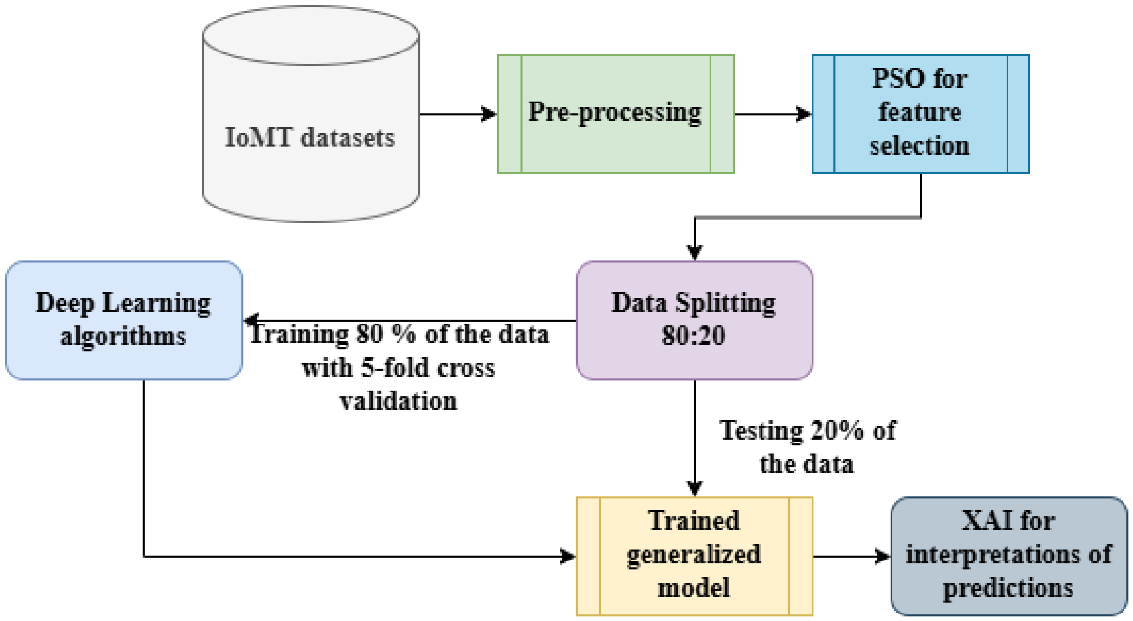
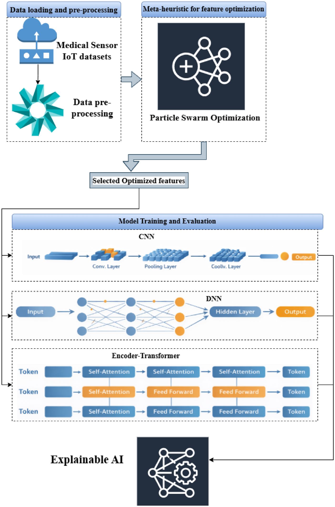
The proposed method, DeepMedShield-XAI, offers a complete pipeline for smartly analyzing medical IoT sensor data by combining data pretreatment, feature optimization, and advanced DL models with XAI, as shown in Figure 1. The flow chart of the proposed method is given in Figure 2. Raw sensor data is first cleaned and processed to ensure its quality and uniformity. Afterward, the most pertinent features are chosen using a metaheuristic optimization method called particle swarm optimization (PSO), which reduces dimensionality and improves efficiency. To capture spatial, nonlinear, and sequential data patterns, the optimal features are fed into models such as a convolutional neural network (CNN), DNNs, and encoder–transformer models. Lastly, an XAI module is implemented to interpret model predictions, thereby improving transparency, trust, and decision-making in critical healthcare applications.

3.1. Dataset Description and Pre-Processing

The proposed method is evaluated using the two medical IoT datasets, i.e., CICIoMT2024 [28] and IoMT_TrafficData [29].

3.1.1. CICIoMT2024 Dataset

The CICIoMT2024 dataset is used to detect intrusions in IoMT (Internet of Medical Things) settings. By including multi-protocol medical network traffic and a variety of attack scenarios specific to healthcare infrastructures, it expands on earlier CIC datasets. The data collection includes medical device, gateway, and cloud service communications, as well as other network traffic originating from realistic IoMT settings. It detects both legitimate and malicious activity across a variety of attack types, including denial-of-service (DoS), distributed denial-of-service (DDoS), probing, brute force, botnet-based assaults, and data exfiltration efforts. Features derived from flow analysis of packet-level communications are used to represent each instance of traffic. Among these statistical attributes are protocol-specific details, byte rates, packet counts (both forward and backward), flow duration, inter-arrival time, and packet length. The dataset is also appropriate for DL and hybrid intrusion detection models since it contains application-layer characteristics pertinent to medical telemetry. The dataset is categorized into benign and various assault classes, facilitating both binary and multiclass classification tasks.

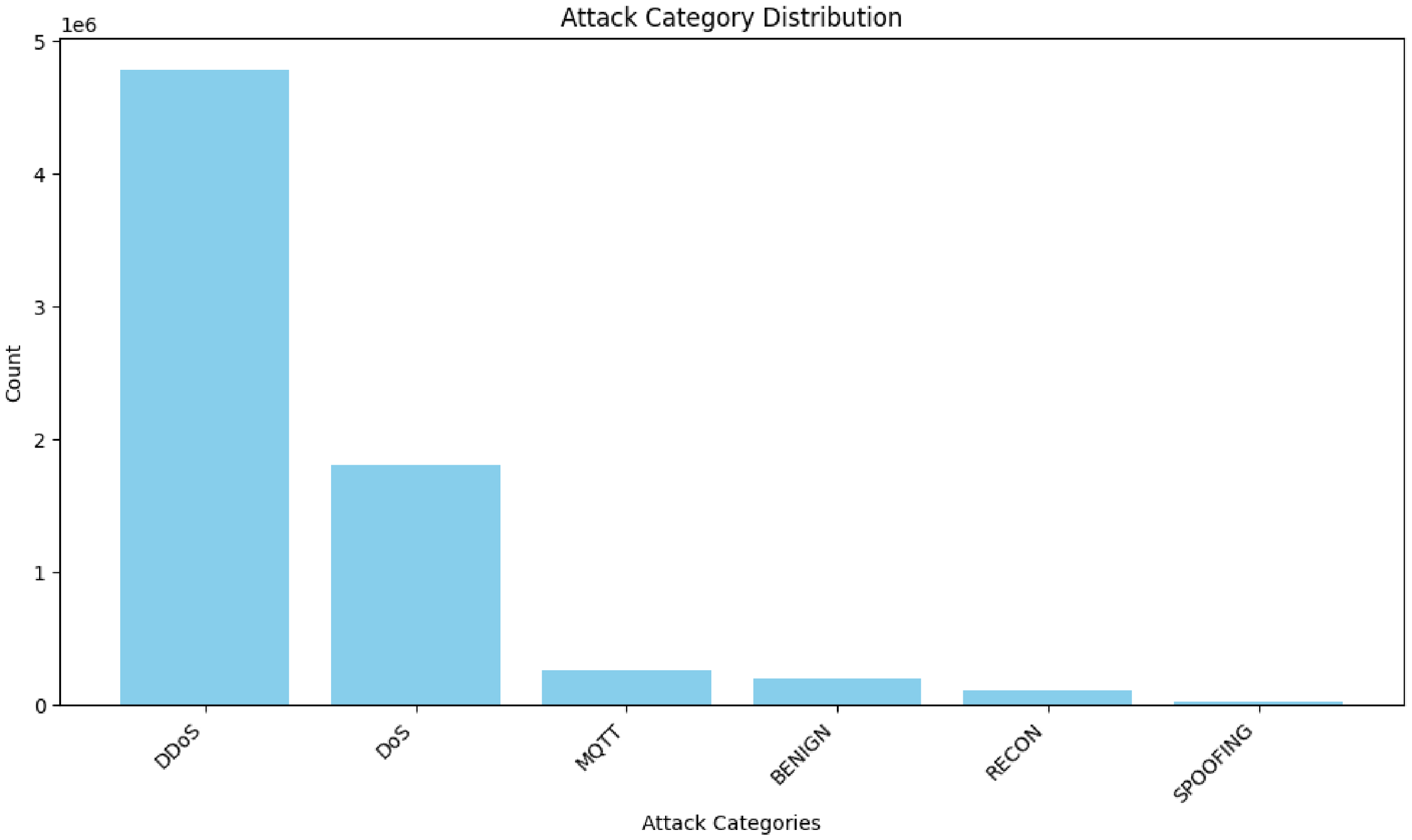
There are 7,160,831 samples and 46 features. There are 51 unique values in the attack label. Thus, the 52 categories are grouped together to form 6 categories. Thus, there are 477,985 samples of DDoS, 180,552 occurrences of DoS, 262,938 of MQTT, 103,726 of recon, 16,047 of spoofing, and 192,732 instances of benign traffic as shown in Figure 3. Thus, the downsampling is performed to reduce the number of samples in the DDoS class to 902,764 and the DoS class to 902,764. Moreover, the dataset does not contain null or infinite values.

3.1.2. IoMT-TrafficData Dataset

The second dataset used is the IoMT-TrafficData dataset, which is an open-source dataset available for intrusion detection in Internet of Medical Things networks. It focuses on recording real-world IoMT communication patterns and attack behaviors in healthcare-related IoT systems. Network traffic generated from medical devices, including wearable sensors, monitoring systems, and connected hospital infrastructure, is included in this dataset. The data indicates both authentic patient monitoring traffic and malicious activity aimed at compromising the confidentiality, integrity, and availability of medical information.

IoMT-TrafficData provides flow-level information gathered from packet grabs, such as statistical, protocol-based, and time-based information. Flow time, packet arrival intervals, forward and backward byte counts, packet sizes, and connection status are all common features. By utilizing these characteristics, models are able to acquire knowledge of both short-term abnormalities and long-term behavioral deviations. Normal traffic and several attack types (such as denial-of-service, scanning, spoofing, and attempted unauthorized access) are tagged in the dataset.

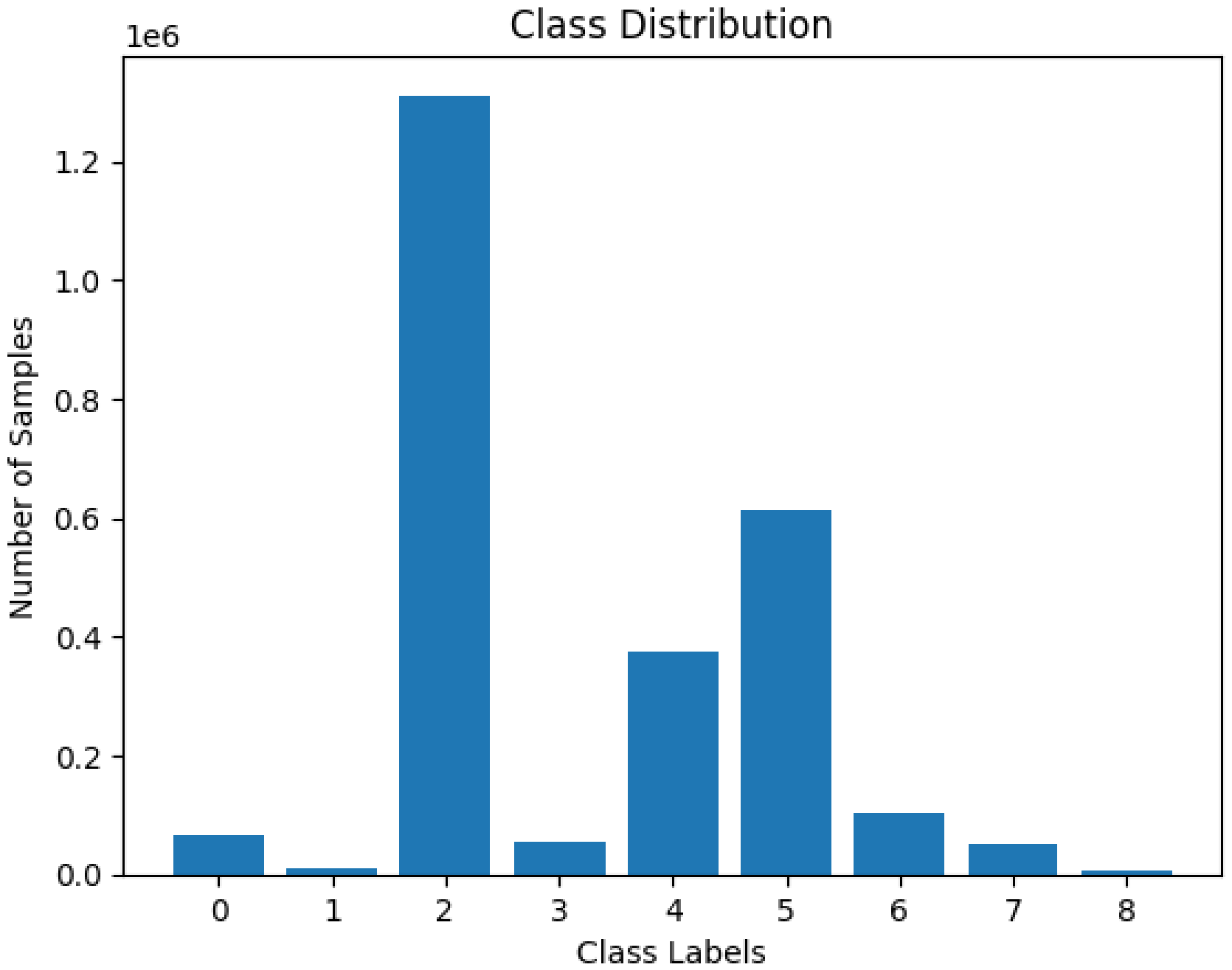
The dataset consists of 3,243,187 samples and 102 features. The 12 features like ‘Unnamed: 0’, ‘id.orig_h’, ‘id.orig_p’, ‘id.resp_h’, ‘id.resp_p’, ‘proto’, ‘service’, ‘conn_state’, ‘history’, ‘local_orig’, ‘local_resp’, ‘tunnel_parents’ are dropped as this information is not useful for training the DL models. Thus, the number of features is 90. The label ‘traffic’ consists of 9 unique values: ‘apachekiller’, ‘arpspoofing’, ‘camoverflow’, ‘mqttmalaria’, ‘netscan’, ‘normal’, ‘rudeadyet’, ‘slowloris’, and ‘slowread’. The label encoder is used to convert the strings into numbers for the target variable ‘traffic’. The dataset is highly imbalanced as shown in Figure 4, where 0 represents ‘apachekiller’, 1 represents ‘arpspoofing’, 2 represents ‘camoverflow’, 3 represents ‘mqttmalaria’, 4 represents ‘netscan’, 5 represents ‘normal’, 6 represents ‘rudeadyet’, 7 represents ‘slowloris’, and 8 represents ‘slowread’.

3.2. Metaheuristic Algorithm for Feature Optimization and Selection

In IDS applications, feature selection is a crucial stage, especially in high-dimensional IoMT datasets where redundant and unnecessary features can impair model performance and raise computational complexity. To solve this problem, a metaheuristic optimization method based on Particle Swarm Optimization (PSO) [30] is used to find the best set of characteristics. PSO is a population-based stochastic optimization method that was inspired by how birds and fish behave when they gather together. Particles in feature selection represent potential solutions stored as binary vectors, with each dimension representing a feature. For features that have been selected, a value of 1 indicates inclusion and a value of 0 indicates exclusion.

Let $x_i=(x_{i1},x_{i2},\dots ,x_{id})$ denote the position of the i-th particle and $v_i=(v_{i1},v_{i2},\dots ,v_{id})$ represent its velocity in a d-dimensional search space. The velocity and position of each particle are updated iteratively as given in Equations (1) and (2).

$$v_i^{t+1}=w{v}_i^t+c_1{r}_1(pbes{t}_i-x_i^t)+c_2{r}_2(gbest-x_i^t)$$

(1)

$$x_i^{t+1}=x_i^t+v_i^{t+1}$$

(2)

where w is the inertia weight, $c_1$ and $c_2$ are acceleration coefficients, and $r_1,r_2\in [0,1]$ are random values. The terms $pbes{t}_i$ and $gbest$ denote the personal best and global best positions, respectively.

For binary feature selection, the velocity is transformed using a sigmoid activation function as given in Equation (3).

$$S\left(v_i\right)={\displaystyle \frac{1}{1+e^{-v_i}}}$$

(3)

A threshold is then applied to determine whether a feature is selected.

The fitness function is designed to balance classification performance and feature reduction as given in Equation (4).

$$Fitness=\alpha ·Acc+(1-\alpha )\left(1-{\displaystyle \frac{|F_{selected}|}{|F_{total}|}}\right)$$

(4)

where $Acc$ represents the classification accuracy, $|F_{selected}|$ is the number of selected features, $|F_{total}|$ is the total number of features, and $\alpha \in [0,1]$ controls the trade-off.

The PSO method updates particles over and over until it reaches a stopping point, like the maximum number of iterations or convergence. The final classification model is subsequently trained using the optimal feature subset, which enhances detection accuracy and decreases computational complexity. The algorithm for the PSO is defined in Algorithm 1.

Algorithm 1 Particle Swarm Optimization (PSO) for Feature Selection

1: Input: Swarm size $N=20$, maximum iterations $T=15$ 2: Parameters: $c_1=2.0$, $c_2=2.0$, $w=0.7$, neighborhood size $k=15$, Minkowski order $p=2$ 3: Initialize particle positions ${\mathbf{x}}_i$ and velocities ${\mathbf{v}}_i$ for $i=1,\dots ,N$ 4: Initialize personal best ${\mathbf{p}}_i={\mathbf{x}}_i$ 5: Determine global best $\mathbf{g}$ among all particles 6: for $t=1$ to T do 7:      for $i=1$ to N do 8:           Evaluate fitness $f\left({\mathbf{x}}_i\right)$ 9:           if $f\left({\mathbf{x}}_i\right)<f\left({\mathbf{p}}_i\right)$ then 10:                ${\mathbf{p}}_i\leftarrow {\mathbf{x}}_i$ 11:         end if 12:         if $f\left({\mathbf{x}}_i\right)<f\left(\mathbf{g}\right)$ then 13:                $\mathbf{g}\leftarrow {\mathbf{x}}_i$ 14:         end if 15:         for each dimension d do 16:                Update velocity: 17:                $v_{i,d}^{t+1}=w·v_{i,d}^t+c_1{r}_1(p_{i,d}-x_{i,d}^t)+c_2{r}_2(g_d-x_{i,d}^t)$ 18:                Update position: 19:                $x_{i,d}^{t+1}=x_{i,d}^t+v_{i,d}^{t+1}$ 20:         end for 21:     end for 22: end for 23: Return global best solution $\mathbf{g}$

The number of features selected by PSO from the CICIoMT2024 dataset is 16. The features selected are ‘protocol type’, ‘duration’, ‘Srate’, ‘ack_flag_number’, ‘ece_flag_number’, ‘cwr_flag_number’, ‘syn_count’, ‘fin_count’, ‘SSH’, ‘IRC’, ‘IGMP’, ‘IPv’, ‘IAT’, ‘number’, ‘covariance’, and ‘variance’. However, the number of features selected from the IoMT_TrafficData dataset is 42.

3.3. DL Methods

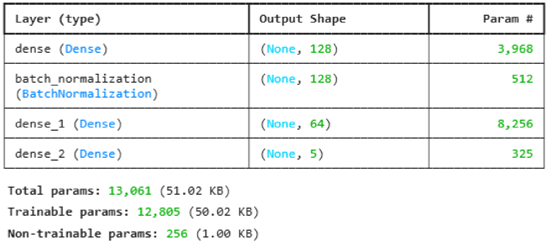
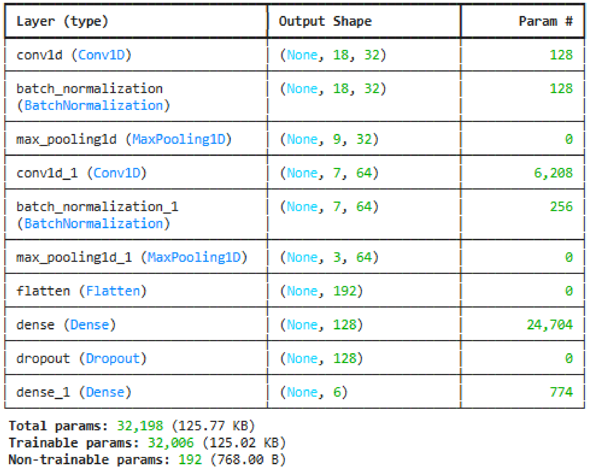
The PSO-optimized features are trained using DNN, CNN, and the hybrid encoder–transformer model. The CNN model, as shown in Figure 5, has three dense layers and one batch normalization. The CNN model, as shown in Figure 6, has 2 convolution layers, two batch normalization layers, two max-pooling layers, one flatten, two dense and one dropout. The encoder–transformer model includes an input layer, 4 dense layers, two multi-head attention layers, several normalization blocks, including approximately five layer-normalization blocks and two batch-normalization blocks, and five dropout layers for regularization. It has three residual (i.e., ADD) connections within the encoder blocks in the style of transformers. A global average pooling layer then generates the output representation. Hence, it is a 20-layer hybrid model that combines deep neural network feature extraction with attention-based learning.

The robust performance of all models, i.e., DNN, CNN, and encoder–transformer, is ensured by training them for up to 200 epochs using five-fold cross-validation. To ensure sustained learning and efficient computation, we use a batch size of 2. By ceasing training when validation performance reaches a plateau, overfitting can be prevented with a 20-epoch patience for early stopping. To ensure steady convergence, the learning rate (LR) is set to 0.0001 for the DNN and encoder–transformer. On the other hand, the LR is optimized with a higher rate of 0.001, which is utilized for the CNN.

3.4. Explainable AI

The model predictions are interpreted, and the features responsible for each class are identified using XAI techniques. Both local and global interpretability are provided in this work through the use of LIME (Local Interpretable Model-agnostic Explanations) [31] and SHAP (SHapley Additive exPlanations) [32]. In the vicinity of a specific instance, LIME approximates the complex model $f\left(x\right)$ with a more easily understood model $g\left(x\right)$ to explain particular predictions. The objective function of LIME is defined in Equation (5).

$$\mathcal{L}(f,g,{\pi }_x)+\mathsf{\Omega }\left(g\right)$$

(5)

where $\mathcal{L}(f,g,{\pi }_x)$ measures the fidelity of the surrogate model g to the original model f within the locality defined by ${\pi }_x$, and $\mathsf{\Omega }\left(g\right)$ represents the complexity of the interpretable model. This formulation enables the identification of locally important features contributing to a specific class prediction.

SHAP, based on cooperative game theory, assigns each feature a contribution value known as the Shapley value. For a prediction function $f\left(x\right)$, the SHAP value ${\varphi }_i$ for feature i is given in Equation (6).

$${\varphi }_i=\sum _{S\subseteq F\setminus \left\{i\right\}}{\displaystyle \frac{\left|S\right|!\left(\right|F|-|S|-1)!}{\left|F\right|!}}\left[f(S\cup \{i\left\}\right)-f\left(S\right)\right]$$

(6)

where F is the set of all features and S represents a subset of features excluding feature i. This formulation ensures a fair distribution of feature contributions by considering all possible feature subsets.

The proposed framework combines both instance-level explanations and global feature importance assessments by merging LIME and SHAP. This allows for the selection of essential features that are responsible for improving the reliability of the IDS in IoT devices.

3.5. Robustness Analysis with Fast Gradient Sign Method (FGSM) and Projected Gradient Descent (PGD) Adversarial Attack

FGSM [33] is a popular benchmark for assessing adversarial resilience in IDS applications. This method generates small perturbations by maximizing the prediction error while maintaining imperceptible modifications to the original samples by utilizing the sign of the gradient of the loss function with respect to the input features. The FGSM Accuracy measures the model’s classification accuracy under the FGSM adversarial attack, which assesses the model’s robustness against single-step perturbation-based attacks. The FGSM drop measure shows the extent of model vulnerability to hostile attacks by showing the drop in classification accuracy when the FGSM is changed, compared with normal test accuracy. FGSM generates adversarial samples using the formula in Equation (7).

$$x_{\mathrm{adv}}=x+ϵ·\mathrm{sign}\left({\nabla }_{x}J(\theta ,x,y)\right)$$

(7)

where x represents the original input sample, $x_{\mathrm{adv}}$ denotes the adversarial sample, $ϵ$ is the perturbation magnitude controlling the attack strength, $\theta$ represents the model parameters, y is the true class label, and $J(\theta ,x,y)$ denotes the loss function of the model.

Moreover, the PGD [34] attack is a stronger iterative extension of FGSM and is often used as a standard robustness test in research on adversarial learning. PGD generates progressively difficult attack samples by applying gradient-based perturbations in an iterative manner while simultaneously projecting adversarial samples inside a limited perturbation region. PGD generates adversarial samples iteratively using formulae in Equation (8).

$$x_{t+1}={\mathsf{\Pi }}_{ϵ}\left(x_t+\alpha ·\mathrm{sign}\left({\nabla }_{x}J(\theta ,x_t,y)\right)\right)$$

(8)

where $x_t$ represents the adversarial sample at iteration t, $\alpha$ denotes the step size, $ϵ$ defines the maximum perturbation bound, ${\mathsf{\Pi }}_{ϵ}$ projects the perturbed sample into the allowable perturbation region, $\theta$ represents the model parameters, y is the true class label, and $J(\theta ,x_t,y)$ denotes the loss function of the model.

The out-of-distribution (OOD) detection rate [35] is also evaluated, which gives a measure of the model’s capacity to detect OOD samples that deviate from the original training data distribution. In conventional benchmark datasets, OOD evaluation is often accomplished by introducing previously unseen or distribution-shifted samples and assessing the proportion of correctly identified anomalous inputs, which indicates the model’s generalization and dependability in real-world deployment circumstances. The Out-of-Distribution (OOD) detection score is computed using the maximum softmax probability as given in Equation (9).

$$\mathrm{OOD}\mathrm{Score}\left(x\right)=1-\underset{i}{max}\left(P(y_i\mid x)\right)$$

(9)

where $P(y_i\mid x)$ represents the predicted softmax probability for the $y_i$ class given input sample x. Higher OOD scores indicate a greater likelihood that the input sample does not belong to the training data distribution.

3.6. Evaluation Metrics

The various evaluation metrics used for IDS systems are accuracy, as given in Equation (10), precision as given in Equation (11), recall as given in Equation (12), F1-score as given in Equation (13), area under receiver operating characteristics (AUC-ROC) as given in Equation (14) and precision–recall AUC as given in Equation (15). TP is true positive, TN is true negative, FP is false positive, FN is false negative, TPR is the true positive rate, which is the same as recall, and FPR is the false positive rate.

A more robust analysis is performed by evaluating performance using balanced accuracy (Bal_ACC) as given in Equation (16), Matthews correlation coefficient (MCC) as given in Equation (17), kappa as given in Equation (18), G-mean as given in Equation (19), Jaccard index as given in Equation (19), and Dice coefficient as given in Equation (21).

$$\mathrm{Accuracy}={\displaystyle \frac{TP+TN}{TP+TN+FP+FN}}$$

(10)

$$\mathrm{Precision}={\displaystyle \frac{TP}{TP+FP}}$$

(11)

$$\mathrm{Recall}={\displaystyle \frac{TP}{TP+FN}}$$

(12)

$$F1={\displaystyle \frac{2·\mathrm{Precision}·\mathrm{Recall}}{\mathrm{Precision}+\mathrm{Recall}}}$$

(13)

$$\mathrm{AUC}\text{-}\mathrm{ROC}={\int }_0^1\mathrm{TPR}\left(x\right)d\left(\mathrm{FPR}\left(x\right)\right)$$

(14)

$$\mathrm{PR}\text{-}\mathrm{AUC}={\int }_0^1\mathrm{Precision}\left(r\right)dr$$

(15)

$$\mathrm{Bal}\text{\_}\mathrm{Acc}={\displaystyle \frac{1}{2}}\left({\displaystyle \frac{TP}{TP+FN}}+{\displaystyle \frac{TN}{TN+FP}}\right)$$

(16)

$$\mathrm{MCC}={\displaystyle \frac{(TP\times TN)-(FP\times FN)}{\sqrt{(TP+FP)(TP+FN)(TN+FP)(TN+FN)}}}$$

(17)

$$\mathrm{Kappa}={\displaystyle \frac{\left(\frac{TP+TN}{TP+TN+FP+FN}\right)-\left(\frac{(TP+FP)(TP+FN)+(FN+TN)(FP+TN)}{{(TP+TN+FP+FN)}^2}\right)}{1-\left(\frac{(TP+FP)(TP+FN)+(FN+TN)(FP+TN)}{{(TP+TN+FP+FN)}^2}\right)}}$$

(18)

$$\mathrm{G}\text{-}\mathrm{Mean}=\sqrt{\left({\displaystyle \frac{TP}{TP+FN}}\right)\left({\displaystyle \frac{TN}{TN+FP}}\right)}$$

(19)

$$\mathrm{Jaccard}\mathrm{Index}={\displaystyle \frac{TP}{TP+FP+FN}}$$

(20)

$$\mathrm{Dice}\mathrm{Coefficient}={\displaystyle \frac{2TP}{2TP+FP+FN}}$$

(21)

4. Results

The experiments are performed using the open-source cloud platform Kaggle on an NVIDIA P100 GPU. The five-fold cross-validation results of the proposed three models, i.e., DNN, CNN, and encoder–transformer (ET) models on the CICIoMT2024 and IoMT_TrafficData datasets are shown in

Table 1. Five-fold cross-validation results with training time.

Dataset	Model	Fold	Accuracy (%)	Precision (%)	Recall (%)	F1-Score (%)	Epochs	Time (m)
CICIoMT	DNN	1	99.63	91.41	89.86	90.56	99	74.25
		2	99.61	91.15	89.66	90.34	90	69
		3	99.71	93.40	93.10	93.24	150	120
		4	99.69	92.32	93.02	92.63	166	132.8
		5	99.64	91.66	90.36	90.96	146	116.8
		Mean ± Std	99.65 ± 0.04	91.99 ± 0.90	91.20 ± 1.72	91.55 ± 1.30	-	512.85
	CNN	1	78.94	77.52	83.02	79.33	23	22.61
		2	78.78	78.02	80.99	77.84	21	21
		3	76.23	76.81	78.31	73.23	22	22
		4	75.30	74.73	74.77	66.87	21	21
		5	74.65	75.82	76.83	70.55	22	22
		Mean ± Std	76.78 ± 1.98	76.58 ± 1.32	78.79 ± 3.28	73.56 ± 5.14	-	108.61
	ET	1	99.12	90.40	88.76	89.49	62	84.73
		2	99.29	90.44	88.47	89.33	29	39.63
		3	99.44	90.76	88.73	89.62	65	88.83
		4	99.43	90.56	88.49	89.38	23	31.05
		5	99.50	90.91	90.99	90.91	39	55.9
		Mean ± Std	99.36 ± 0.15	90.61 ± 0.22	89.09 ± 1.07	89.75 ± 0.66	-	300.14
IoMT	DNN	1	99.89	98.97	99.20	99.09	47	16.45
		2	99.87	98.59	99.26	98.92	30	10.5
		3	99.86	98.90	99.03	98.96	43	15.05
		4	99.87	98.65	99.21	98.92	33	11.05
		5	99.88	99.17	98.98	99.07	22	7.7
		Mean ± Std	99.87 ± 0.01	98.86 ± 0.24	99.14 ± 0.12	98.99 ± 0.08	-	60.75
	CNN	1	99.88	99.22	98.85	99.03	38	17.1
		2	99.87	99.26	98.98	99.12	12	5.6
		3	99.87	99.00	99.02	99.01	16	7.4
		4	99.88	99.24	98.97	99.10	13	5.85
		5	99.88	99.06	99.07	99.06	21	9.45
		Mean ± Std	99.88 ± 0.01	99.16 ± 0.12	98.98 ± 0.08	99.06 ± 0.05	-	45.4
	ET	1	99.80	99.00	98.09	98.54	100	141.67
		2	99.81	98.93	98.47	98.70	31	43.92
		3	99.79	98.97	98.02	98.49	62	87.83
		4	99.83	98.91	98.52	98.71	82	116.17
		5	99.83	98.70	98.51	98.59	53	72.25
		Mean ± Std	99.81 ± 0.02	98.90 ± 0.12	98.32 ± 0.25	98.61 ± 0.10	-	461.84

. With an overall accuracy of 99.65%, precision of 91.99%, recall of 91.20%, and F1-score of 91.55%, the DNN model has the best prediction performance for the CICIoMT2024 dataset. However, this efficacy is achieved at the expense of a substantial computational overhead, as evidenced by the high training time of 512.85 min and the large number of epochs up to 166. The encoder–transformer (ET) offers a competitive alternative with a slightly reduced accuracy of 99.36% and an F1-score of 89.75%, while simultaneously reducing the training time to 300.14 min. This represents a moderate trade-off between performance and efficiency. The CNN model, on the other hand, has the worst performance with an accuracy of 76.78% and an F1-score of 73.56%, but it is also the most efficient in terms of time, as it only takes 108.61 min.

All models are efficient on the IoMT dataset. With a total training time of just 45.4 min, the CNN model not only achieves the greatest accuracy of 99.88% and F1-score of 99.06%, but it also surpasses others by a little margin. In a balanced trade-off, the DNN model performs similarly with an accuracy of 99.87% and F1-score of 98.99% but takes 60.75 min to train. In contrast, the ET model, while demonstrating robust performance with an accuracy of 99.81% and F1-score of 98.61%, entails a significantly greater computational expense of 461.84 min, making it less suitable for real-time implementation.

The results underscore a distinct accuracy-time trade-off, as DNN has the highest accuracy on complicated datasets like CICIoMT2024; it also has the largest training cost. CNN, on the other hand, gives the best balance between efficiency and performance, particularly when it comes to IoMT data. Finally, ET offers competitive accuracy, but it comes at a far greater computational expenditure.

The robust evaluation metrics of the DNN, CNN, and ET models on the CICIoMT and IoMT datasets using five-fold cross-validation are shown in

Table 2. Performance analysis of DNN, CNN, and ET models on CICIoMT and IoMT datasets.

Dataset	Model	Fold	Bal_Acc (%)	MCC (%)	Kappa (%)	G-Mean (%)	Jaccard (%)	Dice (%)
CICIoMT	DNN	1	89.87	99.24	99.24	94.76	86.27	90.57
		2	89.66	99.18	99.18	94.65	86.01	90.34
		3	93.08	99.41	99.41	96.45	89.20	93.12
		4	93.02	99.36	99.36	96.41	88.60	92.62
		5	90.36	99.26	99.26	95.02	86.66	90.96
		Mean ± Std	91.20 ± 1.71	99.29 ± 0.09	99.29 ± 0.09	95.46 ± 0.90	87.35 ± 1.45	91.52 ± 1.26
		95% CI	[89.07, 93.32]	[99.17, 99.41]	[99.17, 99.41]	[94.34, 96.57]	[85.55, 89.15]	[89.95, 93.09]
	CNN	1	83.02	56.92	56.92	87.62	69.47	79.33
		2	80.96	54.07	52.51	85.85	68.28	77.81
		3	78.33	48.49	42.37	83.47	64.42	73.22
		4	73.21	40.49	28.83	79.76	55.62	63.43
		5	76.83	45.66	35.74	82.12	62.85	70.55
		Mean ± Std	78.47 ± 3.78	49.13 ± 6.56	43.27 ± 11.59	83.76 ± 3.08	64.13 ± 5.47	72.87 ± 6.34
		95% CI	[73.77, 83.17]	[40.98, 57.27]	[28.88, 57.67]	[79.93, 87.59]	[57.33, 70.93]	[65.00, 80.74]
	ET	1	88.75	98.19	98.19	94.07	84.75	89.49
		2	88.41	98.32	98.32	93.91	84.56	89.28
		3	88.73	98.85	98.85	94.14	85.02	89.62
		4	88.49	98.83	98.83	94.01	84.86	89.38
		5	90.99	98.98	98.98	95.33	86.47	90.91
		Mean ± Std	89.07 ± 1.08	98.64 ± 0.35	98.63 ± 0.35	94.29 ± 0.59	85.13 ± 0.77	89.74 ± 0.67
		95% CI	[87.73, 90.42]	[98.20, 99.07]	[98.19, 99.07]	[93.56, 95.02]	[84.18, 86.08]	[88.91, 90.57]
IoMT	DNN	1	88.25	88.70	87.72	93.16	86.04	87.49
		2	99.25	99.65	99.65	99.61	97.98	98.97
		3	99.01	99.60	99.60	99.48	97.95	98.95
		4	99.18	99.63	99.63	99.57	97.86	98.90
		5	98.96	99.64	99.64	99.46	98.15	99.05
		Mean ± Std	96.93 ± 4.85	97.44 ± 4.89	97.25 ± 5.32	98.26 ± 2.85	95.60 ± 5.34	96.67 ± 5.13
		95% CI	[90.91, 100]	[91.37, 100]	[90.64, 100]	[94.72, 100]	[88.96, 100]	[90.30, 100]
	CNN	1	98.83	99.66	99.66	99.40	98.06	99.01
		2	98.95	99.64	99.64	99.46	98.24	99.10
		3	99.00	99.63	99.63	99.48	98.02	98.99
		4	98.94	99.66	99.66	99.45	98.22	99.09
		5	99.05	99.67	99.67	99.51	98.13	99.04
		Mean ± Std	98.95 ± 0.08	99.65 ± 0.02	99.65 ± 0.02	99.46 ± 0.04	98.13 ± 0.09	99.05 ± 0.05
		95% CI	[98.86, 99.05]	[99.63, 99.67]	[99.63, 99.67]	[99.41, 99.51]	[98.02, 98.25]	[98.99, 99.11]
	ET	1	98.06	99.42	99.41	99.00	97.15	98.53
		2	98.45	99.45	99.44	99.19	97.44	98.68
		3	97.99	99.40	99.40	98.96	97.05	98.47
		4	98.50	99.52	99.52	99.22	97.47	98.69
		5	98.49	99.52	99.52	99.22	97.26	98.58
		Mean ± Std	98.30 ± 0.25	99.46 ± 0.06	99.46 ± 0.06	99.12 ± 0.13	97.27 ± 0.18	98.59 ± 0.10
		95% CI	[97.99, 98.61]	[99.39, 99.53]	[99.39, 99.53]	[98.95, 99.28]	[97.05, 97.50]	[98.47, 98.71]

. The analysis includes balanced accuracy (Bal_Acc), Matthews Correlation Coefficient (MCC), Cohen’s Kappa, G-Mean, Jaccard Index, and Dice coefficient, as well as the mean ± standard deviation and 95% confidence intervals (CIs). The DNN model did the best overall on the CICIoMT dataset, with a balanced accuracy of 91.20 ± 1.71%, an MCC of 99.29 ± 0.09%, a Kappa of 99.29 ± 0.09%, a G-Mean of 95.46 ± 0.90%, a Jaccard Index of 87.35 ± 1.45%, and a Dice coefficient of 91.52 ± 1.26%. This shows that the model is very stable and consistent across folds.

The ET model achieved competitive results with 89.07 ± 1.08% balanced accuracy and 98.64 ± 0.35% MCC, while the CNN model had worse performance in MCC (49.13 ± 6.56%) and Kappa (43.27 ± 11.59%), indicating less classification stability. Conversely, all models demonstrated significantly enhanced performance on the IoMT dataset. The CNN model demonstrated the highest performance, with a balanced accuracy of 98.95 ± 0.08%, MCC of 99.65 ± 0.02%, Kappa of 99.65 ± 0.02%, G-Mean of 99.46 ± 0.04%, Jaccard Index of 98.13 ± 0.09%, and Dice coefficient of 99.05 ± 0.05%. The ET model was closely followed by the CNN model, with a balanced accuracy of 98.30 ± 0.25% and an MCC of 99.46 ± 0.06%. In spite of the DNN model’s good IoMT performance, its broader confidence intervals and bigger standard deviation show more variability among folds because of its poor performance in Fold 1. Overall, the findings show that the proposed approach with CNN on IoMT and DNN and ET on CICIoMT offers very robust and dependable classification performance across several validation folds.

The test results comparison is given in

Table 3. Test performance comparison of DNN, CNN, and ET models (in %).

Dataset	Model	Accuracy (%)	Precision (%)	Recall (%)	F1-Score (%)	ROC-AUC
CICIoMT2024	DNN	99.68	91.99	91.15	91.54	0.9999
CICIoMT2024	CNN	76.78	76.58	78.79	73.5	0.9592
CICIoMT2024	ET	99.35	90.56	89.01	89.72	0.9981
IoMT	DNN	99.87	99.05	98.95	98.99	0.9998
IoMT	CNN	99.87	98.97	99.04	99.00	0.9999
IoMT	ET	99.82	98.72	98.51	98.60	0.9984

. The DNN model does the best overall on the CICIoMT2024 dataset, with the highest accuracy of 99.68%, precision of 91.99%, recall of 91.15%, and F1-score of 91.54%. This shows that it is very good at capturing complicated and varied traffic patterns. While the CNN model performs noticeably worse, achieving only 76.78% accuracy and 73.5% F1-score, indicating limited efficacy in handling complex feature relationships in this dataset, the ET model offers competitive performance with slightly lower values, i.e., accuracy of 99.35% and F1-score of 89.72%.

Conversely, the IoMT dataset exhibits near-perfect classification performance for all models. The CNN model somewhat surpasses others with an F1-score of 99.00% and exhibits competitive accuracy at 99.87%, closely behind the DNN model, which has an F1-score of 98.99%. Compared to CNN and DNN, the ET model displays somewhat lower recall of 98.51%, but it still performs well with an accuracy of 99.82% and F1-score of 98.60%.

Thus, the findings indicate that DNNs are more successful for complicated datasets like CICIoMT2024, although CNN obtains slightly greater performance on IoMT_TrafficData. IoMT’s high metrics across all parameters suggest it is easier to classify than CICIoMT2024.

4.1. CICIoMT2024

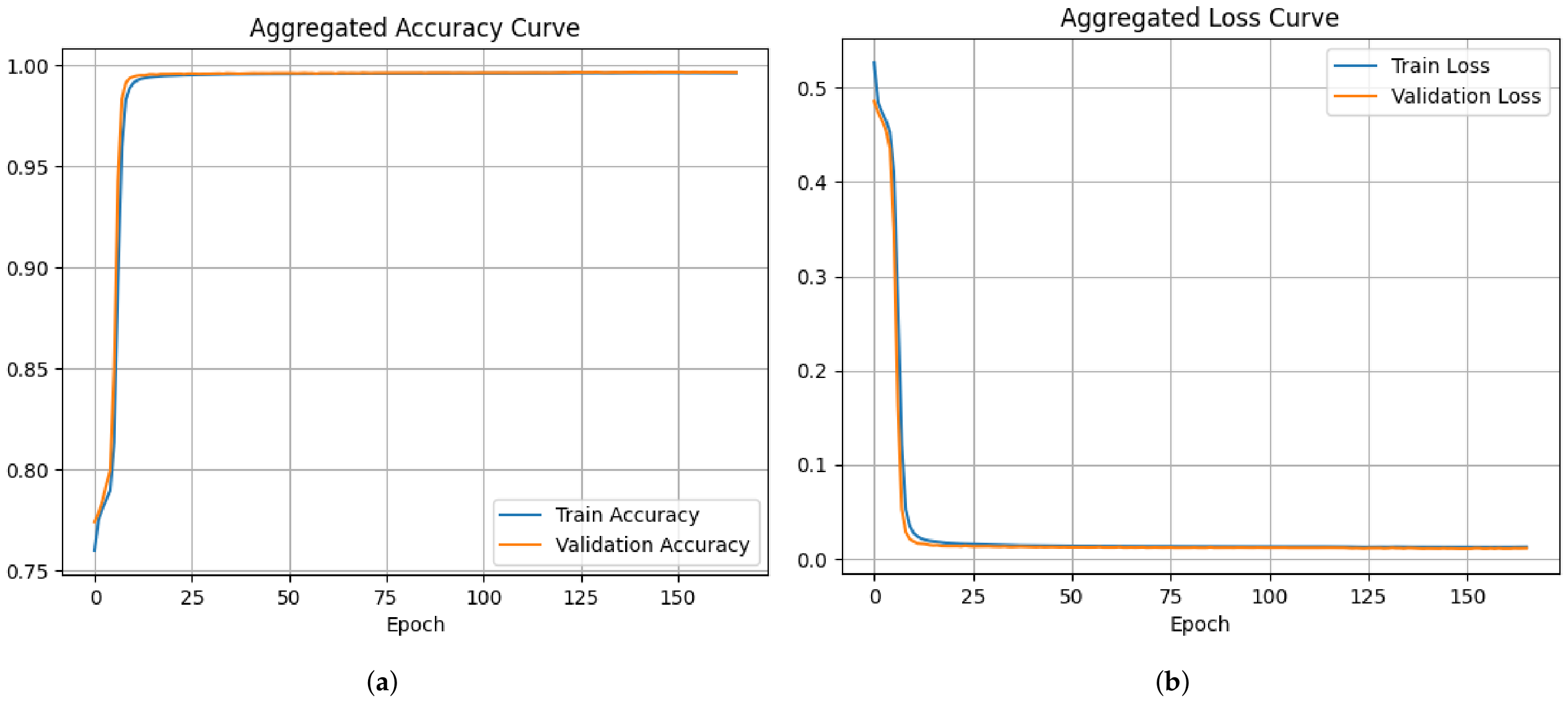
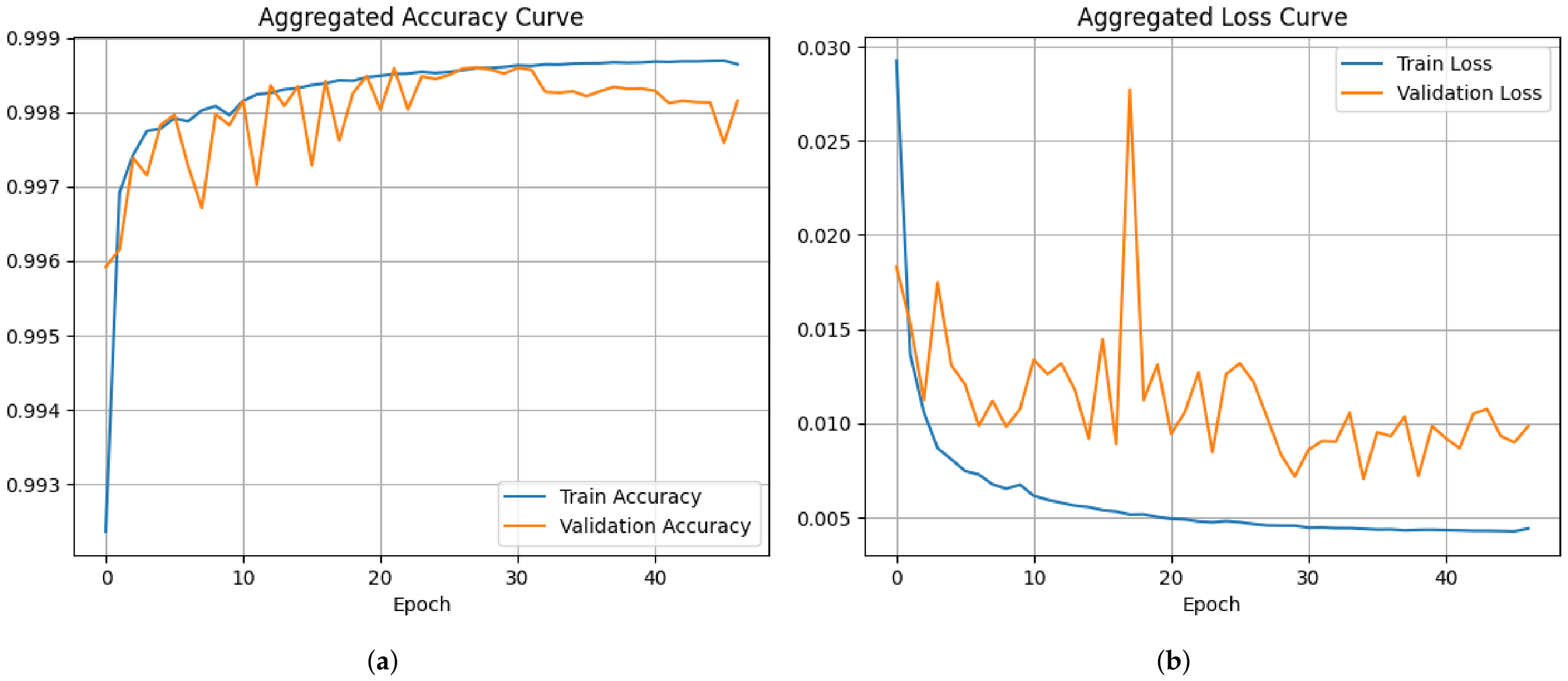
The accuracy and loss curves of the DNN model on the CICIoMT2024 dataset are given in Figure 7a and Figure 7b, respectively. The aggregated accuracy curve Figure 7a demonstrates that the accuracy of both training and validation increases swiftly from approximately 79% in early epochs to above 99.5% within the first 10–15 epochs, ultimately stabilizing at 99.68%. The negligible gap between training and validation accuracy confirms a robust generalization without overfitting. The aggregated loss curve is shown in Figure 7b, with a rapid drop in the training loss from approximately 0.50 to less than 0.02 and a similar pattern in the validation loss, which stabilizes at approximately 0.01. This steady decrease and convergence show that optimization is working well and learning is stable.

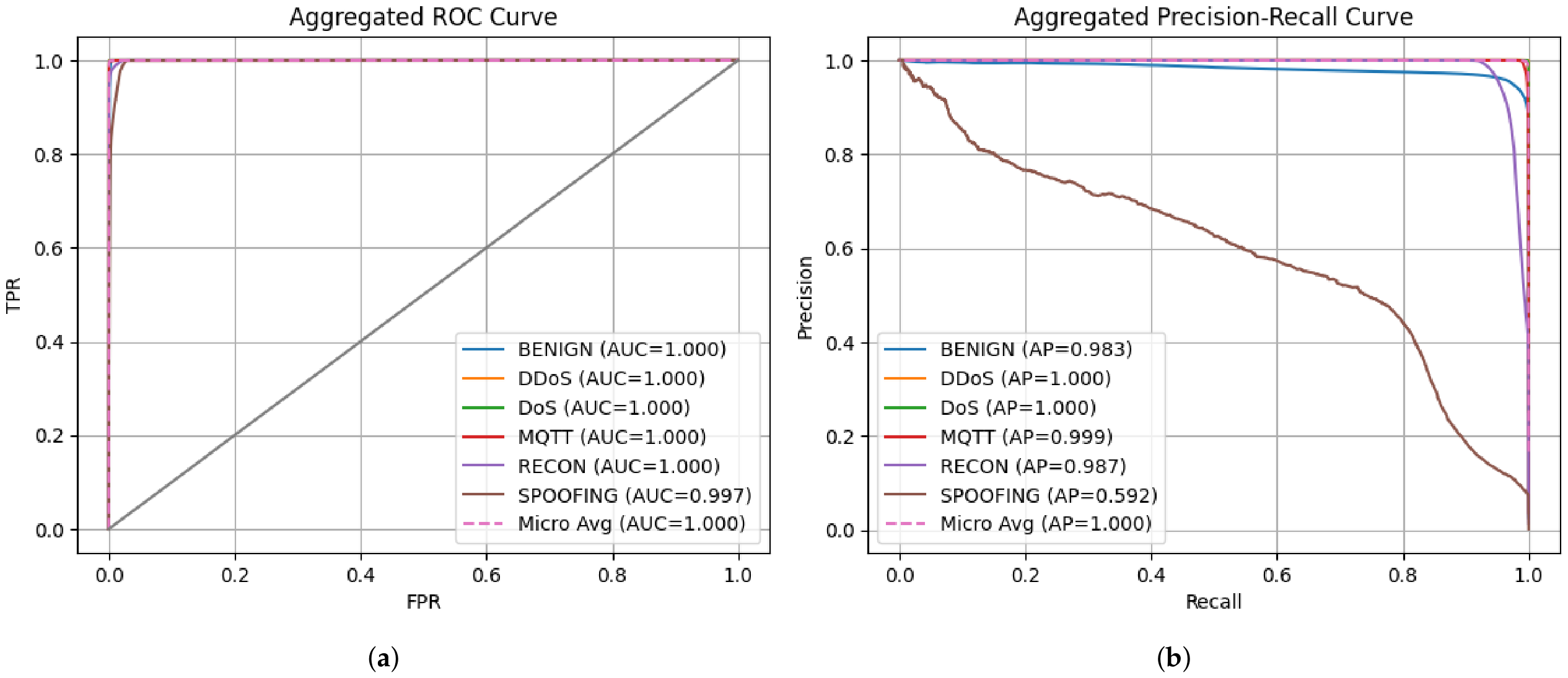
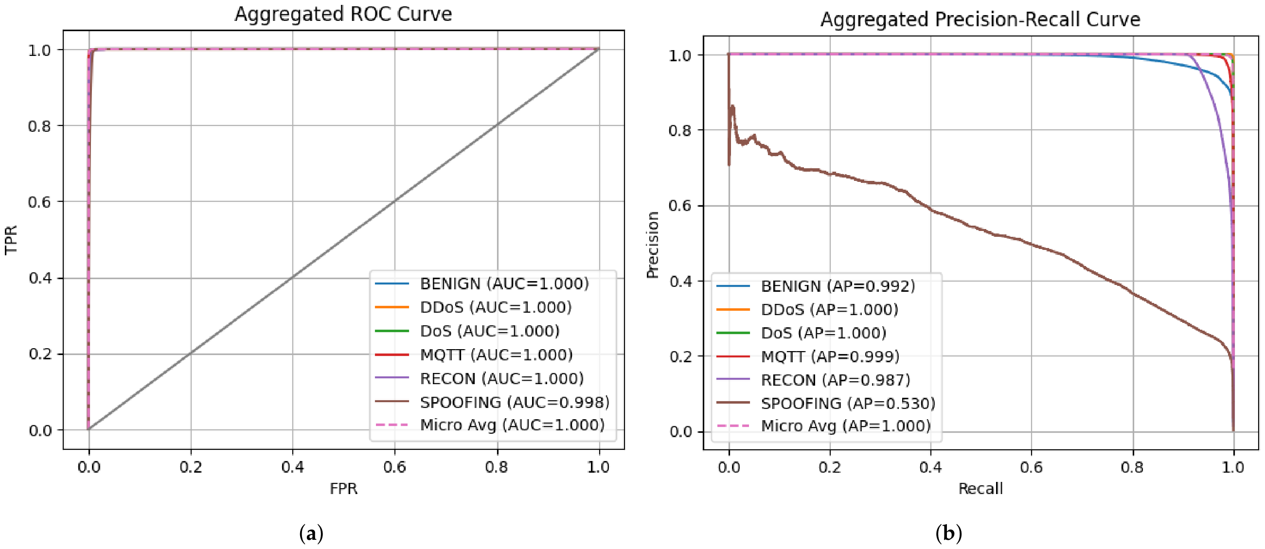
The classification performance is additionally assessed using ROC and precision–recall (PR) curves in Figure 8a and Figure 8b, respectively, for the DNN model on the CICIoMT2024 dataset. The ROC curves for the majority of classes, such as DDoS, DoS, MQTT, and recon, in Figure 8a, accomplish an AUC of 1.000. Spoofing, on the other hand, exhibits a slightly lower AUC of 0.997, which still suggests near-perfect separability. Excellent overall discrimination is confirmed by the micro-average AUC of 1.000. The PR curves in Figure 8b show that the DDoS, DoS, and MQTT classes all get an average precision (AP) of 1.000. The benign class gets an AP of 0.983, and the recon class gets an AP of 0.987. A lower AP of 0.592 for the spoofing class indicates that it is difficult to identify this class from others, maybe because of imbalance or overlap. Still, the micro-average AP is 1.000, proving the model’s strong categorization performance. Together, these findings demonstrate that the DNN model achieves good class-wise discrimination, near-zero loss, and high accuracy, with only modest restrictions in more complicated attack categories like spoofing.

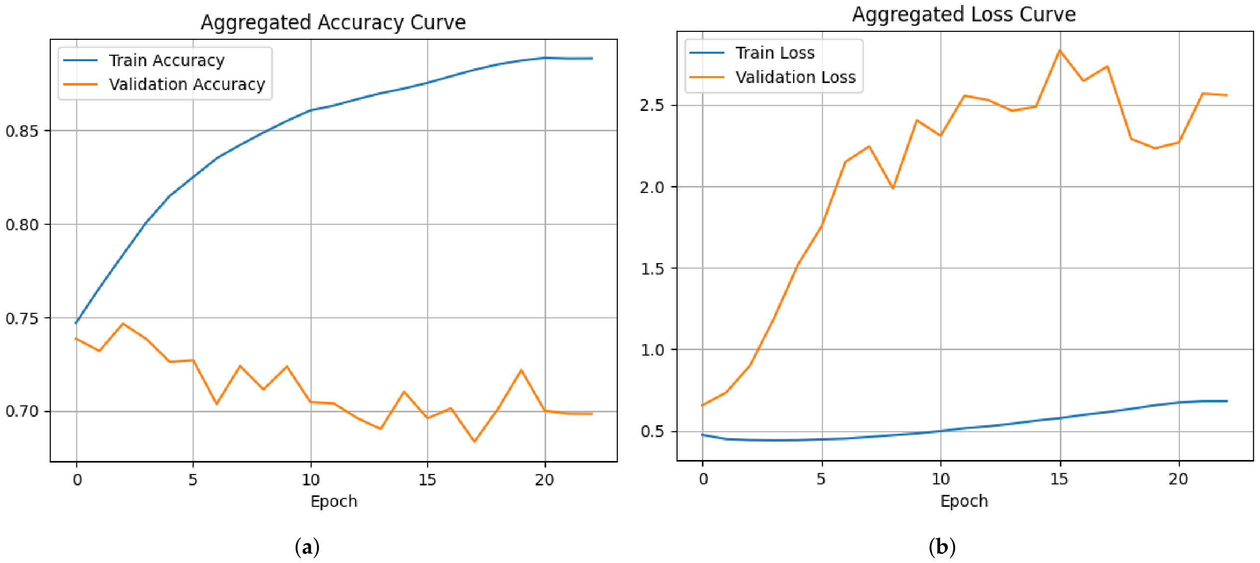
The aggregated accuracy curve of the CNN model on the CICIoMT2024 dataset, given in Figure 9a, illustrates that the training accuracy increases progressively from approximately 75% to approximately 88–89%, suggesting a consistent learning process. Nevertheless, the validation accuracy varies from approximately 68% to 75% and does not exhibit a consistent rising trend, indicating potential overfitting and inadequate generalization. Figure 9b also shows the same trend, demonstrating a rapid decline in both training and validation loss from approximately 0.50 to below 0.02 during the initial epochs, followed by stabilization. Despite low loss values, the validation accuracy inconsistency suggests the model cannot grasp complicated patterns in unseen data.

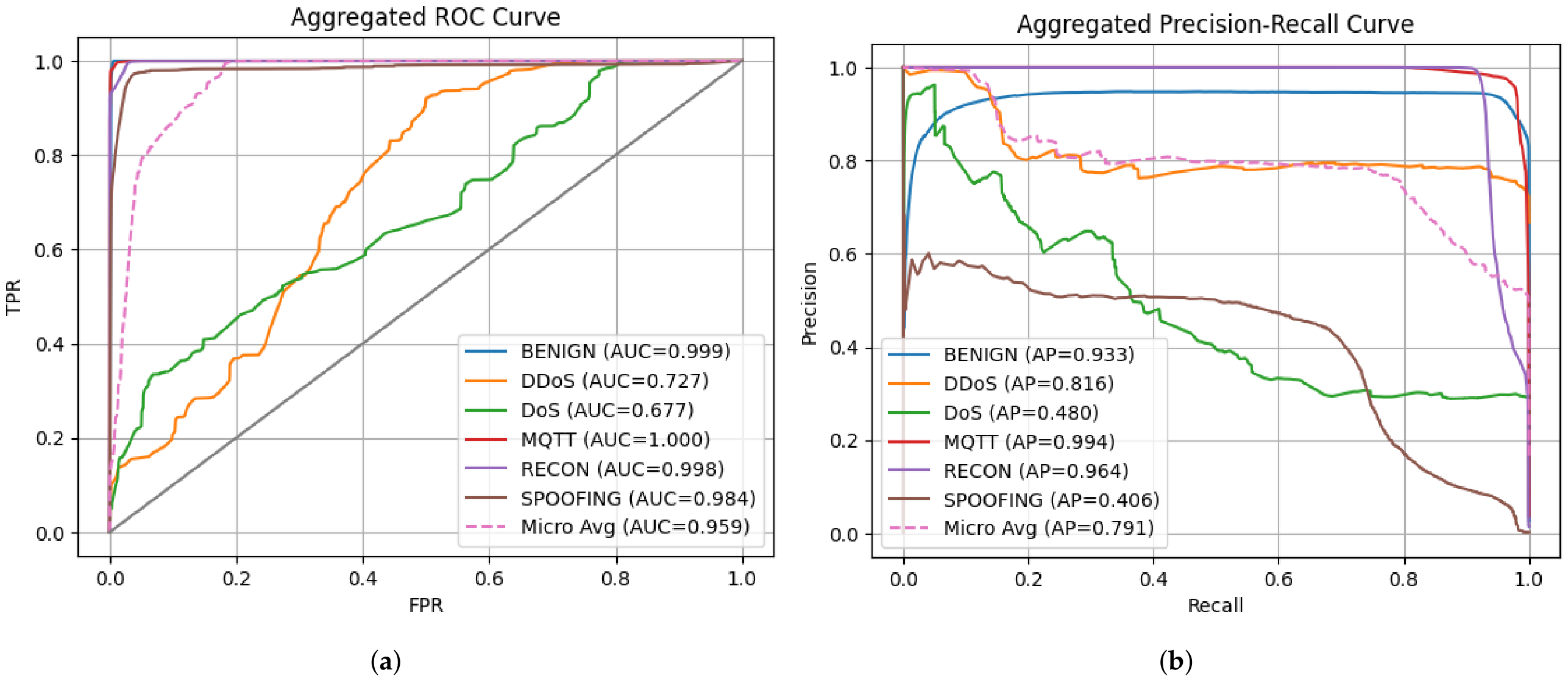
Figure 10 assesses categorization performance through ROC and precision–recall (PR) curves. The ROC plots in Figure 10 show that the benign, with an AUC of 0.999, and MQTT, with an AUC of 1.000, classes do very well. The spoofing class also does very well with an AUC of 0.984. But with DDoS having an AUC of 0.727 and DoS with an AUC of 0.677, performance drastically declines, suggesting that these attacks have poor class separability. The micro-average AUC of 0.959 indicates a moderate overall classification performance. Figure 10b illustrates the performance variation between classes through the PR curves. The benign class obtains a high AP of 0.933, and MQTT is the most effective with an AP of 0.994. However, DDoS with AP of 0.818 has average performance, while DoS with AP of 0.480 and spoofing with AP of 0.406 have much worse precision-recall behavior. With an average performance score AP of 0.791 and a score of 0.594 for the recon class, it is clear that overall performance is far lower than the DNN model.

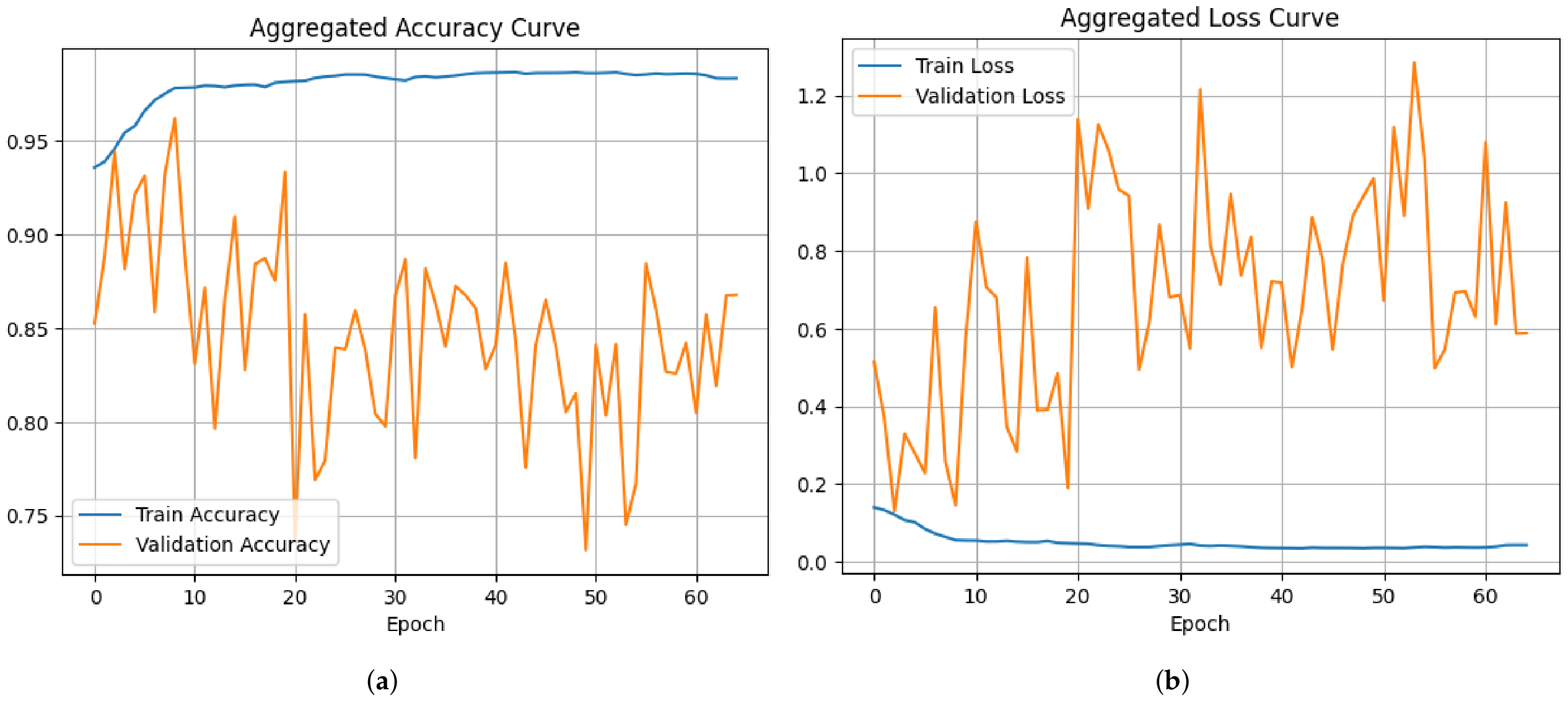
Figure 11 shows the performance of the encoder–transformer (ET) model on the CICIoMT2024 dataset. While the validation accuracy varies greatly between 75% and 90%, suggesting instability and overfitting, the training accuracy given in Figure 11 rapidly reaches 97–98%. In the same way, the training loss stays low, i.e., less than 0.05, but the validation loss, as given in Figure 11b, changes a lot, going up to about 1.2, which shows that the model is not good at generalization.

Regarding classification performance, the ROC curves in Figure 12a for the Encoder-Transformer model on the CICIoMT2024 dataset, demonstrate an almost perfect AUC of 1.000 for the majority of classes and 0.998 for spoofing, which indicates very good separability. With the exception of spoofing, which remains difficult, the PR curves in Figure 12b show strong performance for the majority of classes, with AP values between 0.99 and 1.00. Despite training instability, the micro-average AP of 1.000 indicates good classification performance.

XAI for CICIoMT2024

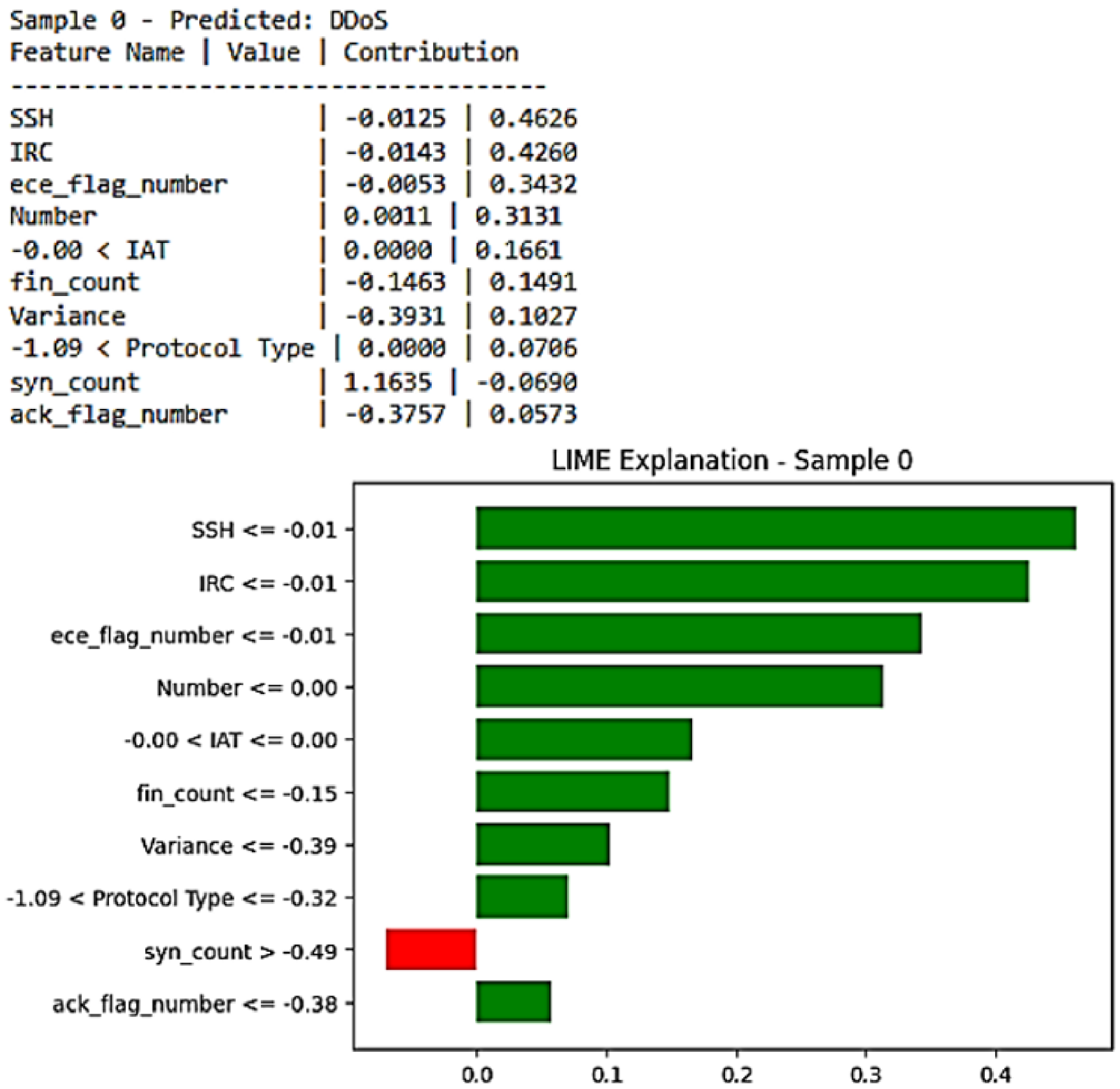
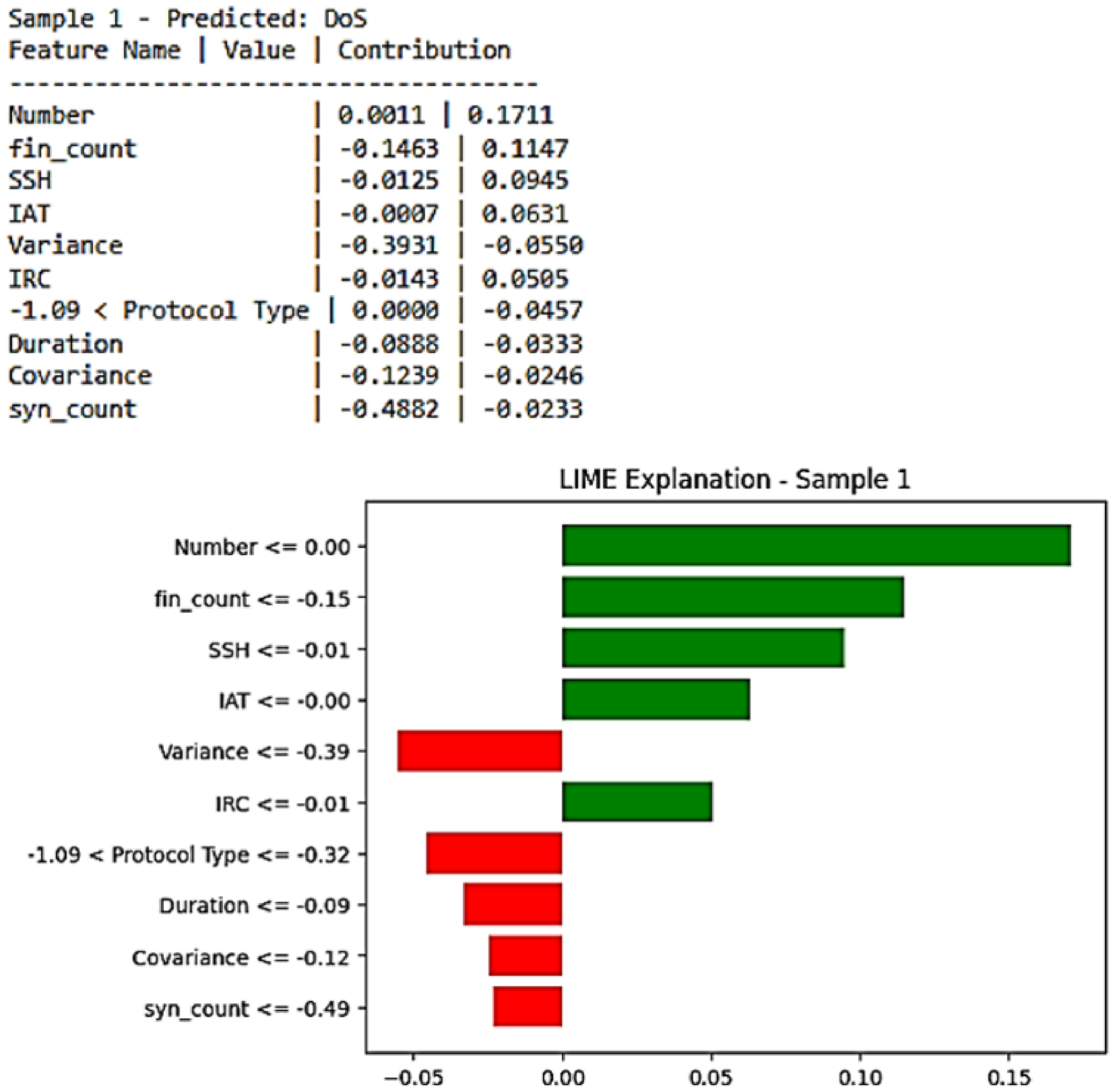
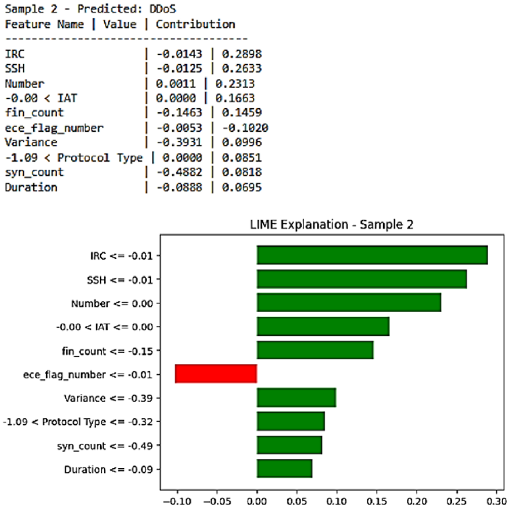
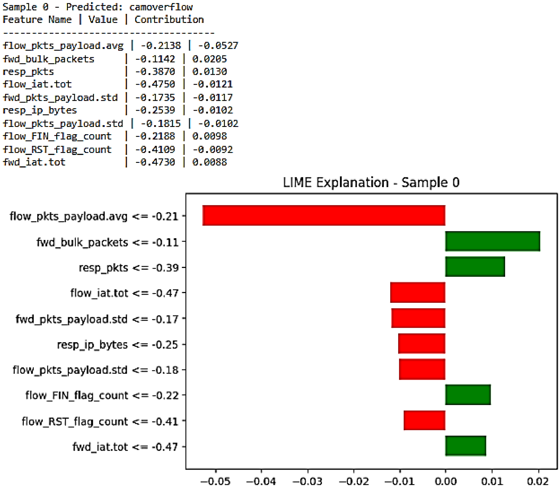
The LIME-based explanation for three samples from the CICIoMT2024 dataset using the DNN model, with a DoS (denial of service) and DDoS forecast, is shown in Figure 13, Figure 14 and Figure 15. Figure 14 shows the value and impact of feature contributions on the prediction. Features exerting a positive influence include number (value = 0.0011, contribution = 0.1711), fin_count (value = −0.1463, contribution = 0.1147), SSH (value = −0.0125, contribution = 0.0945), IAT (value = −0.0007, contribution = 0.0631), and IRC (value = −0.0148, contribution = 0.0505), which significantly propel the prediction towards the DoS class. In contrast, the probability of the DoS prediction is diminished by the following features: variance (value = −0.3931, contribution = −0.0550), protocol type (value = 0.0000, contribution = −0.0457), duration (value = −0.0808, contribution = −0.0333), covariance (value = −0.1239, contribution = −0.0246), and syn_count (value = −0.4882, contribution = −0.0233). The size of these contributions provides an indication of the relative significance of each characteristic. For Figure 13 and Figure 15, the DDoS prediction shows similar feature importance at the sample level; the IRC, SSH, and many other features have a positive impact, while only syn_count and ece_flag_number have a negative impact.

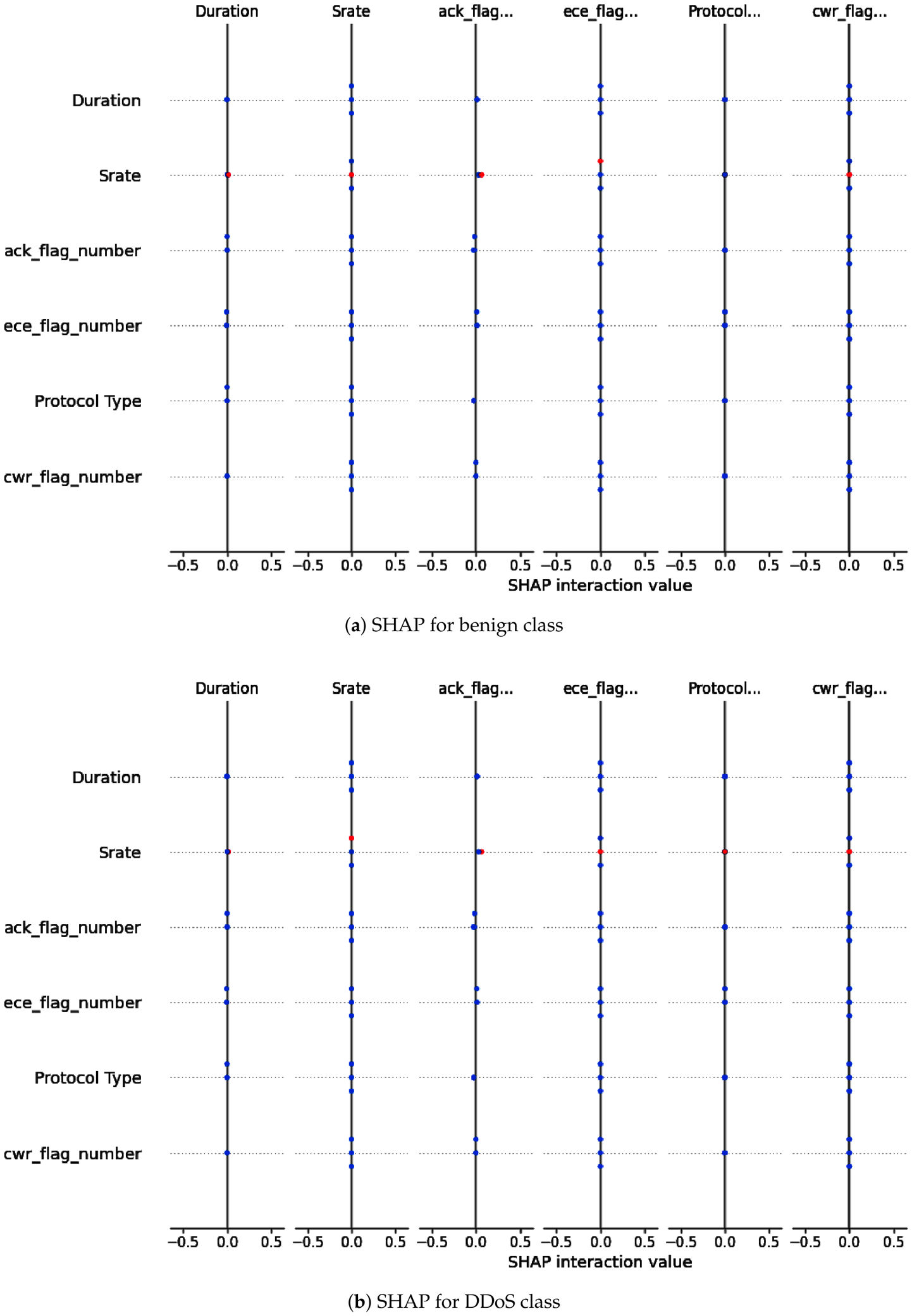
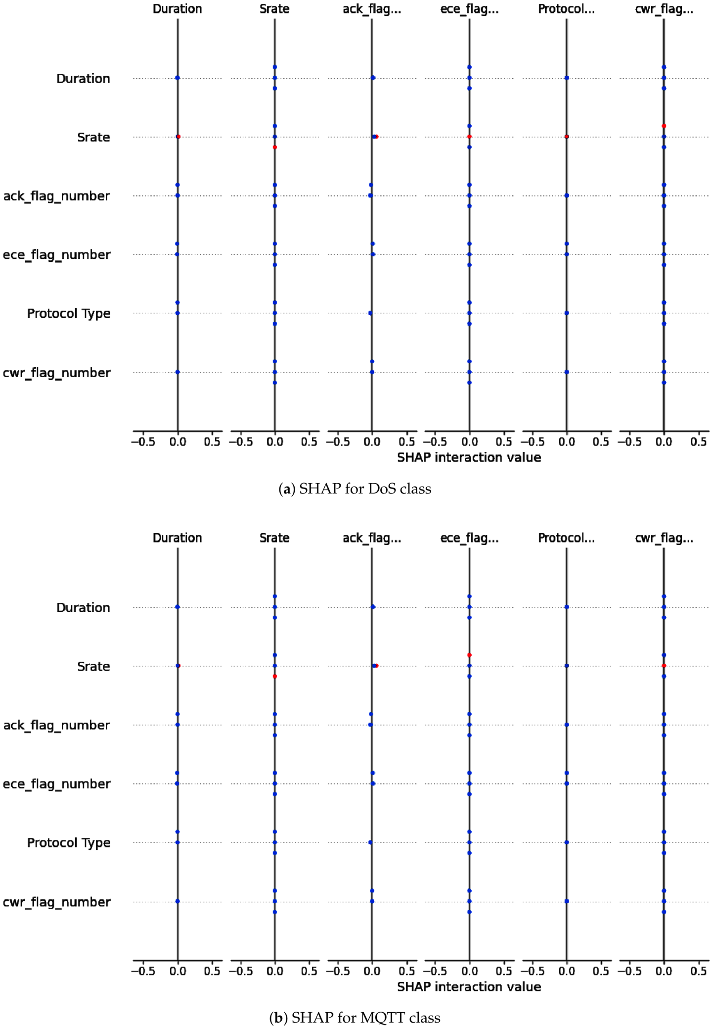
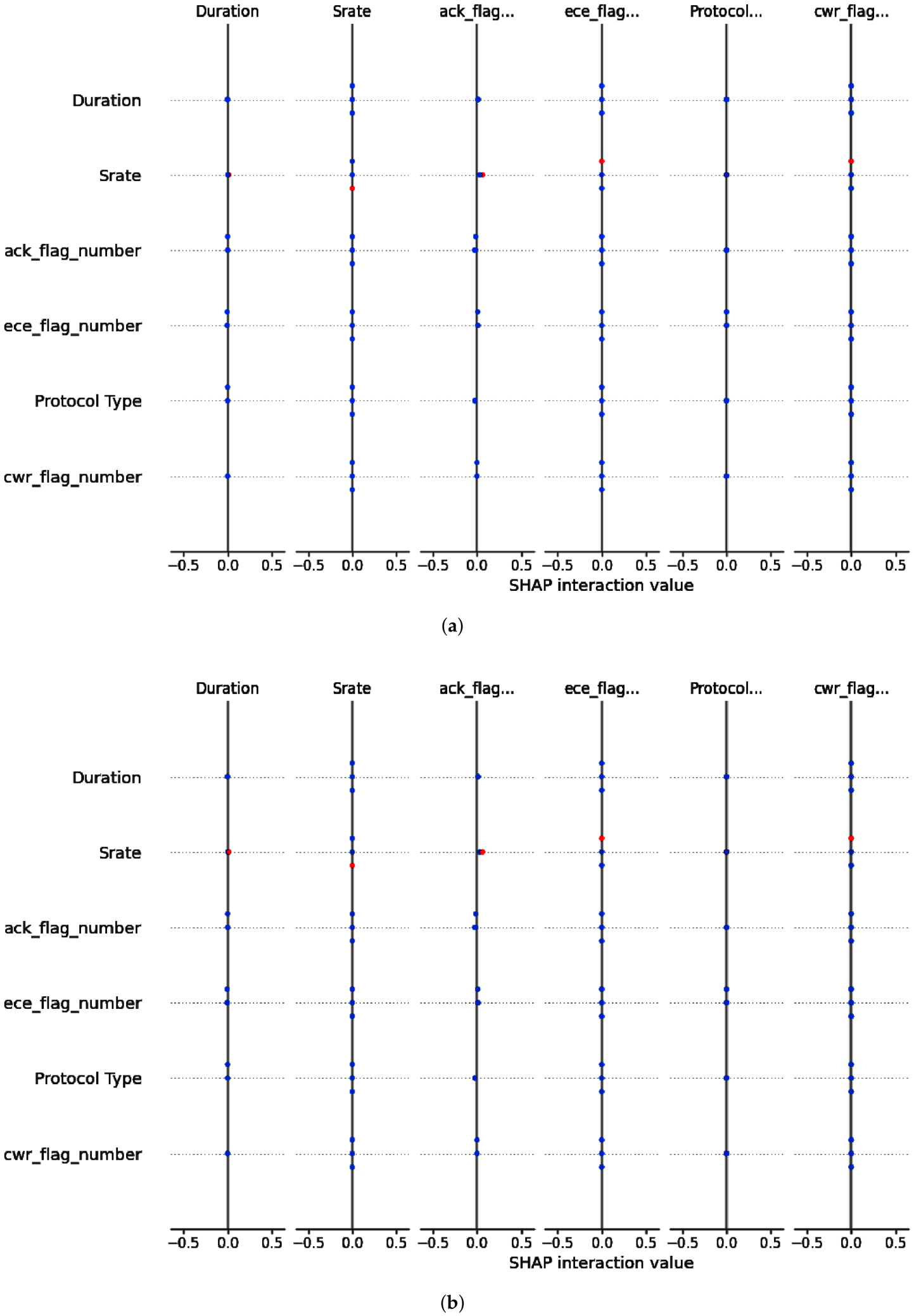
The DNN model’s predictions are jointly influenced by features such as duration, Srate, ack_flag_number, acc_flag_number, protocol type, and cwr_flag_number, as demonstrated by the SHAP interaction plots for the benign class given in Figure 16a, DDoS class given in Figure 16b, DoS class given in Figure 17a, MQTT class given in Figure 17b, recon class given in Figure 18a, and the spoofing class given in Figure 18b. Across all classes, Srate and protocol type exhibit greater and more varied interaction effects, whereas flag-based characteristics have a lesser influence. The benign class is characterized by a high concentration of points near zero, which suggests that traffic behavior is stable and typical.

Conversely, attack classes such as DDoS and DoS exhibit a broader distribution of SHAP interaction values, particularly for duration and Srate, which is indicative of the anomalous and high-intensity traffic patterns. The MQTT class is mostly determined by the protocol type, while the recon and spoofing classes show some variations that are connected to actions like exploring and manipulating. Dots with blue backgrounds indicate low feature values, and red dots with high feature values. Red dots further from zero imply that higher feature values strongly impact the prediction, whereas blue dots grouped around zero indicate that lower values have less impact.

The majority of interaction values are centered around zero in the class-wise interaction plots because the pairwise feature interactions have a limited impact on the prediction for that class. Due to the small number of feature pairs that show significant interaction effects, the model is mostly dependent on the network traffic features alone. This means that the decision boundary for this class is mostly set by direct effects of features, not by complex relationships between features.

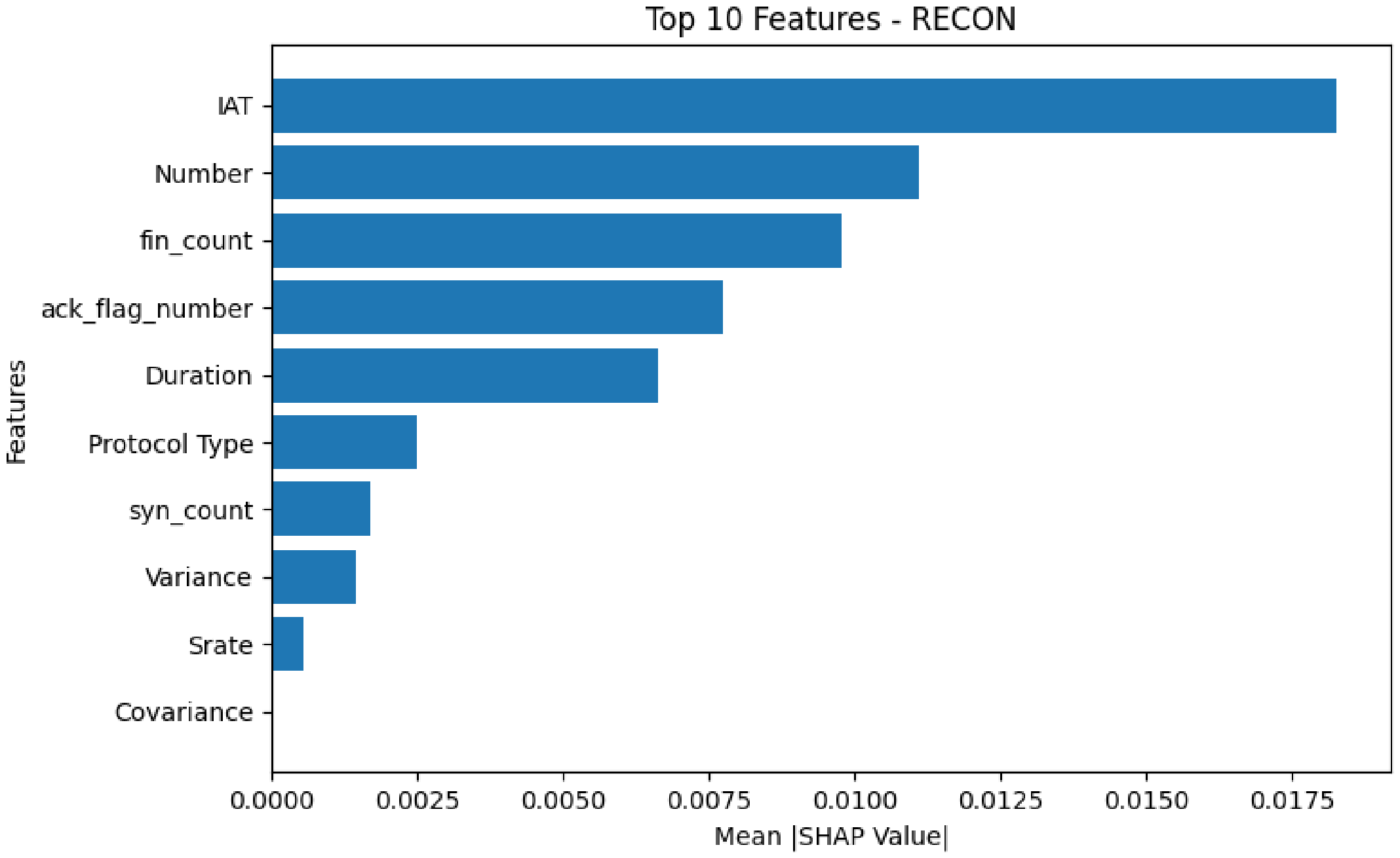
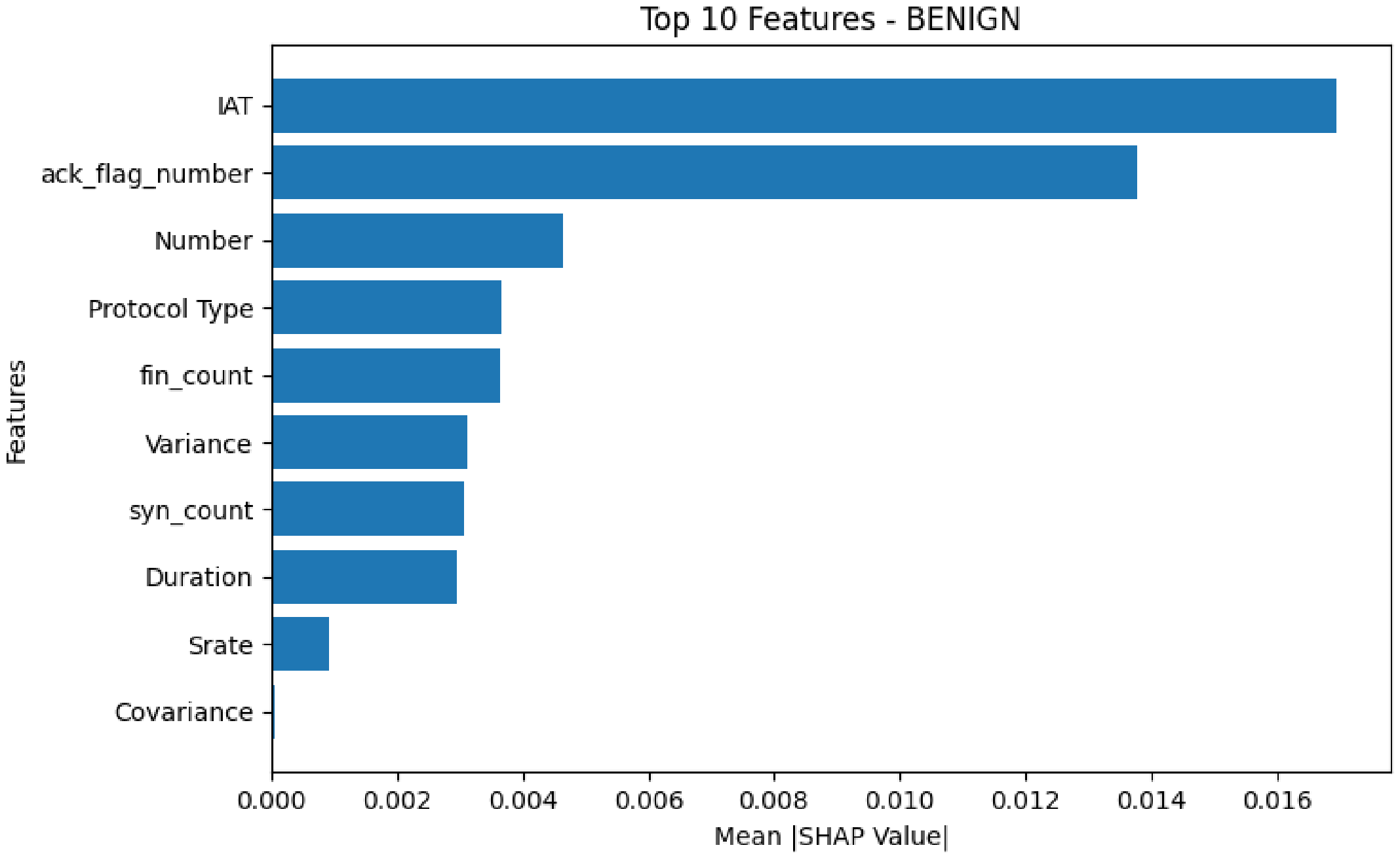
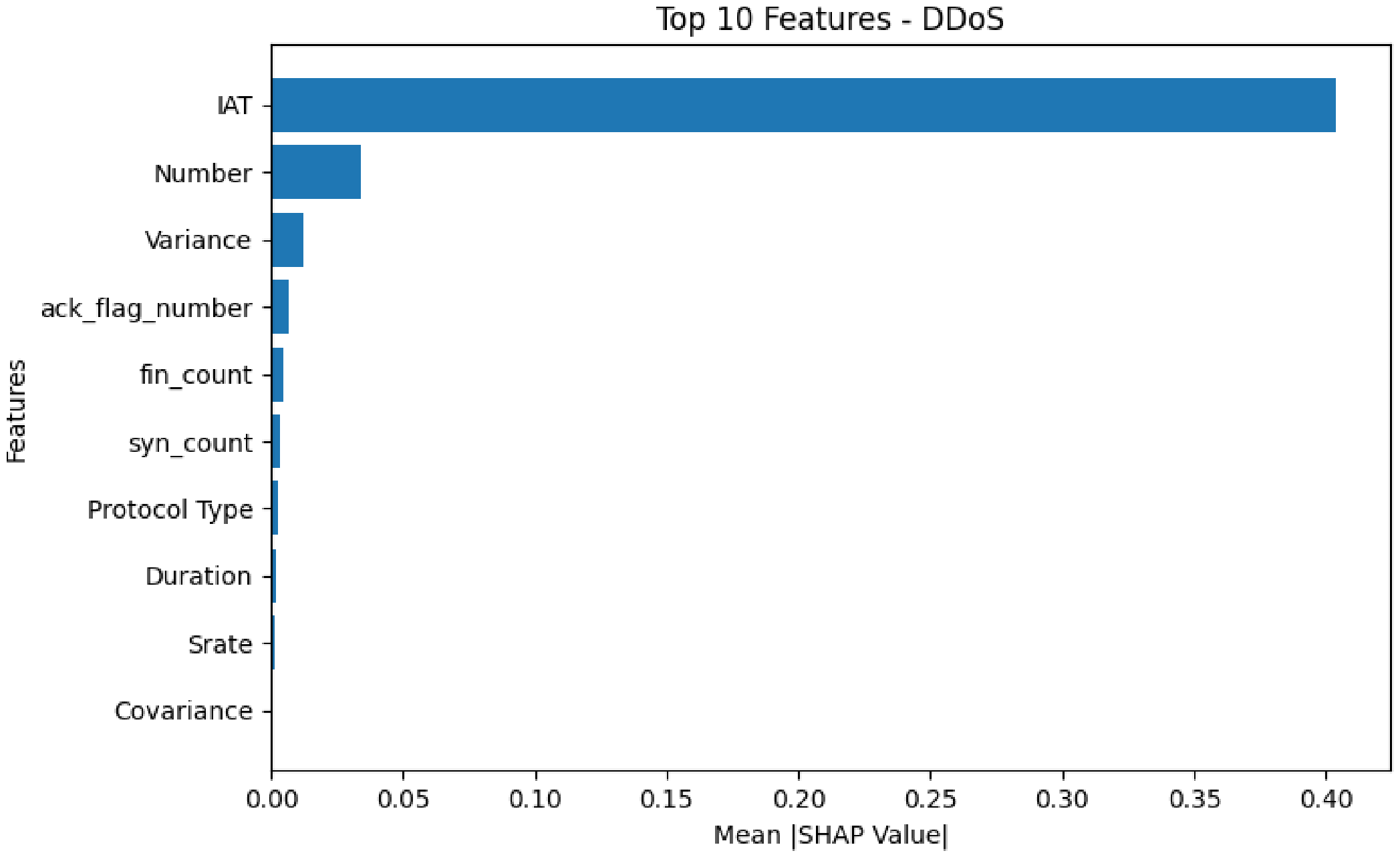
The DNN model distinguishes each class in the CICIoMT2024 dataset by employing a unique set of highly influential features. The benign class is primarily defined by the number of packets, ack_flag_number, and IAT, which are indicative of the stable packet timing and acknowledgment behavior observed in typical traffic as given in Figure 19. IAT is the most important factor in the DDoS class, as shown in Figure 20, and the number of packets and variance show that the attack traffic is bursty and high-volume.

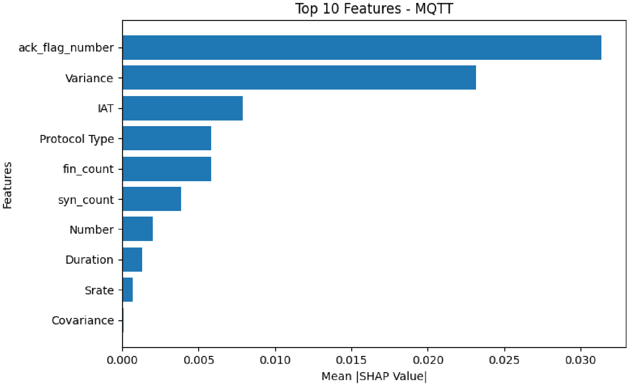
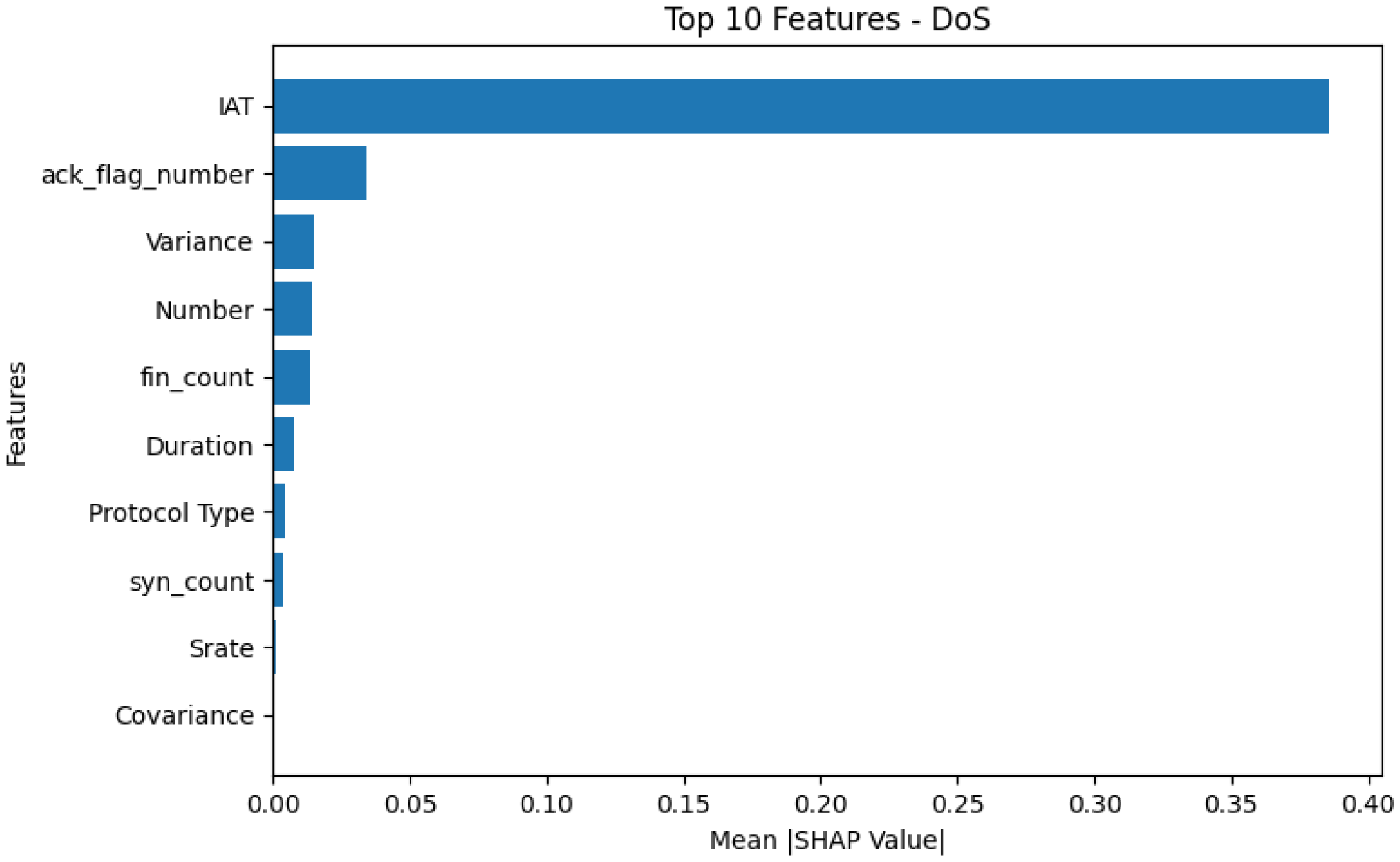
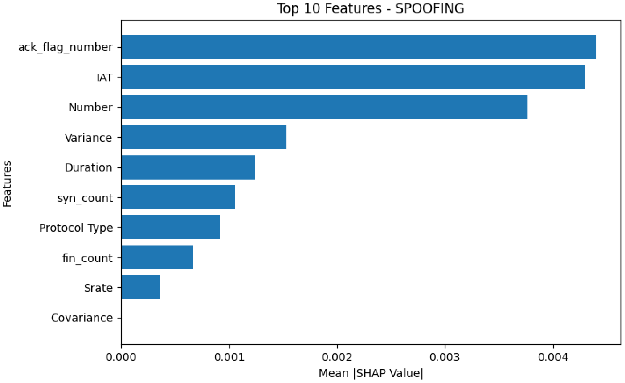
In a similar manner, the IAT, ack_flag_number, and variance are the primary factors that have an impact on the DoS class as shown in Figure 21. These factors indicate anomalous timing and traffic behavior during DoS attacks. The most important features for the MQTT class are ack_flag_number, variance, and IAT, which show connectivity problems that are specific to the protocol as given in Figure 22. In order to capture the probing and scanning patterns of reconnaissance activities, the recon class primarily uses IAT, number of packets, and fin_count as given in Figure 23. Lastly, ack flag number, IAT, and number of packets are the main drivers of the spoofing class as given in Figure 24. These variables represent the unusual acknowledgment behavior and changed traffic characteristics that are associated with faked communications.

4.2. IoMT_TrafficData

The DNN model’s performance on the IoMT_TrafficData dataset is shown in Figure 25. The accuracy of both training and evaluation, as given in Figure 25, quickly converges to about 99.8–99.9%. This shows that learning is stable and that the model works well in real time. Figure 25b shows that the loss curves smoothly decline, with the training loss falling below 0.005 and the validation loss stabilizing around 0.008–0.012, indicating that the convergence is efficient.

After about 15 epochs, the validation loss varies and occasionally spikes, but the training loss continuously declines, indicating a modest propensity toward overfitting in the DNN model. The fact that the overfitting effect is small and has little impact on the model’s generalization is shown by the training and validation accuracies, which are nearly equal.

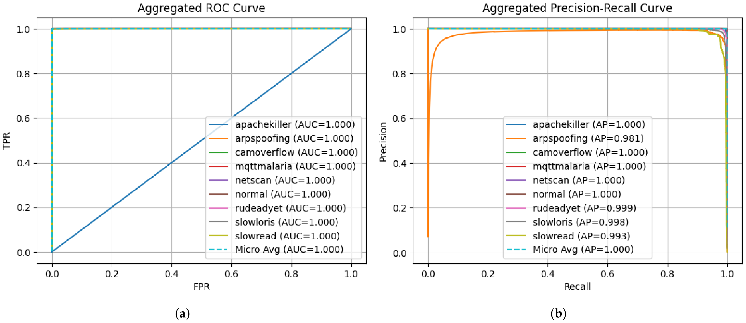
For every class, the ROC curves shown in Figure 26a, reach an AUC of 1.000, indicating flawless class separability. In a similar vein, the PR curves given in Figure 26b, demonstrate an average precision (AP) value of 1.000, indicating almost flawless classification performance, with AP values ranging from 0.99 to 1.00 for all assault types. When tested on the IoMT dataset, the DNN model performs well in classifying all classes.

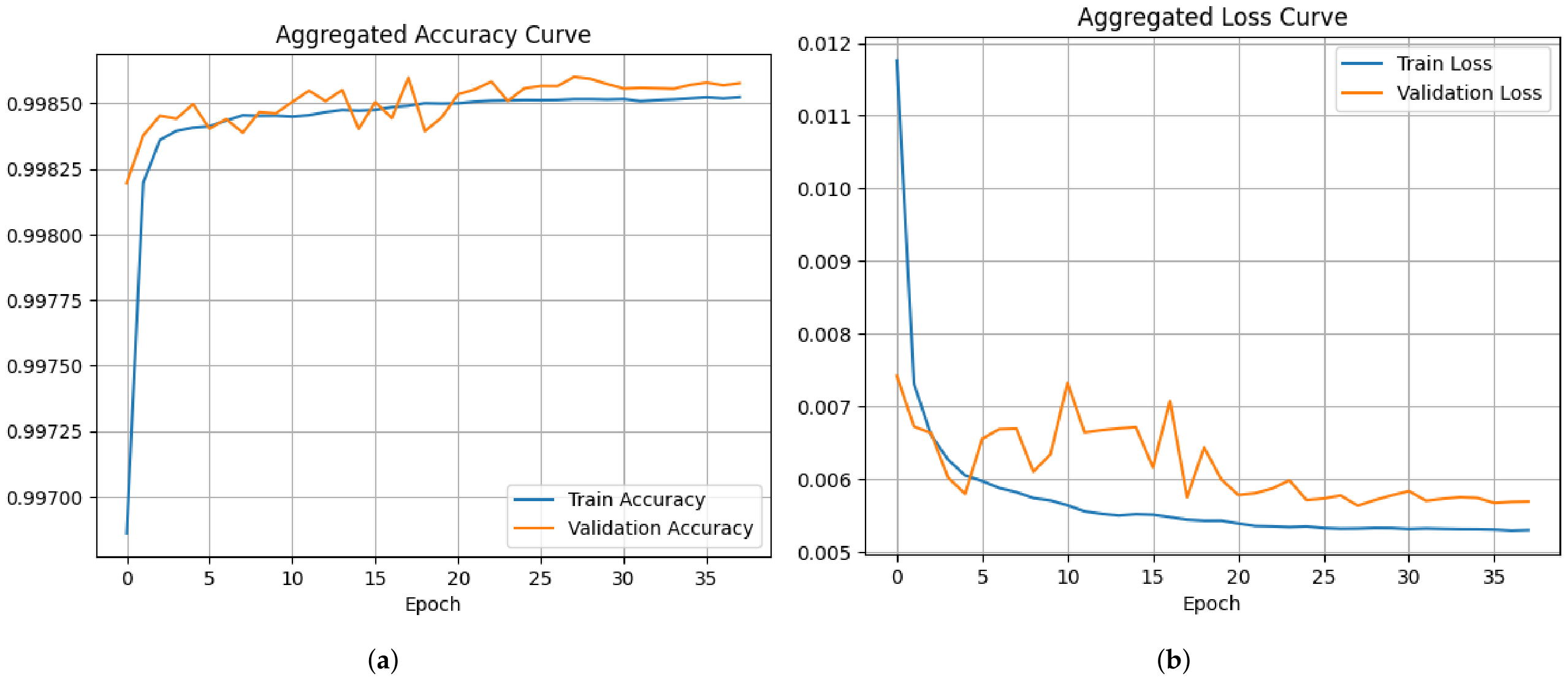
The CNN model’s performance on the IoMT_TrafficData dataset is shown in Figure 27 and Figure 28. The accuracy curves given in Figure 27a, demonstrate that both training and validation accuracy swiftly converge to approximately 99.85–99.90%, exhibiting little variation, which signifies consistent learning and effective generalization. The loss curves, as depicted in Figure 27b, exhibit a gradual decline, wherein the training loss decreases to approximately 0.005, and the validation loss stabilizes near 0.006. The CNN model shows high generalization performance and consistent convergence, with loss curves and training and validation accuracy roughly matching. This indicates that there is minimal overfitting.

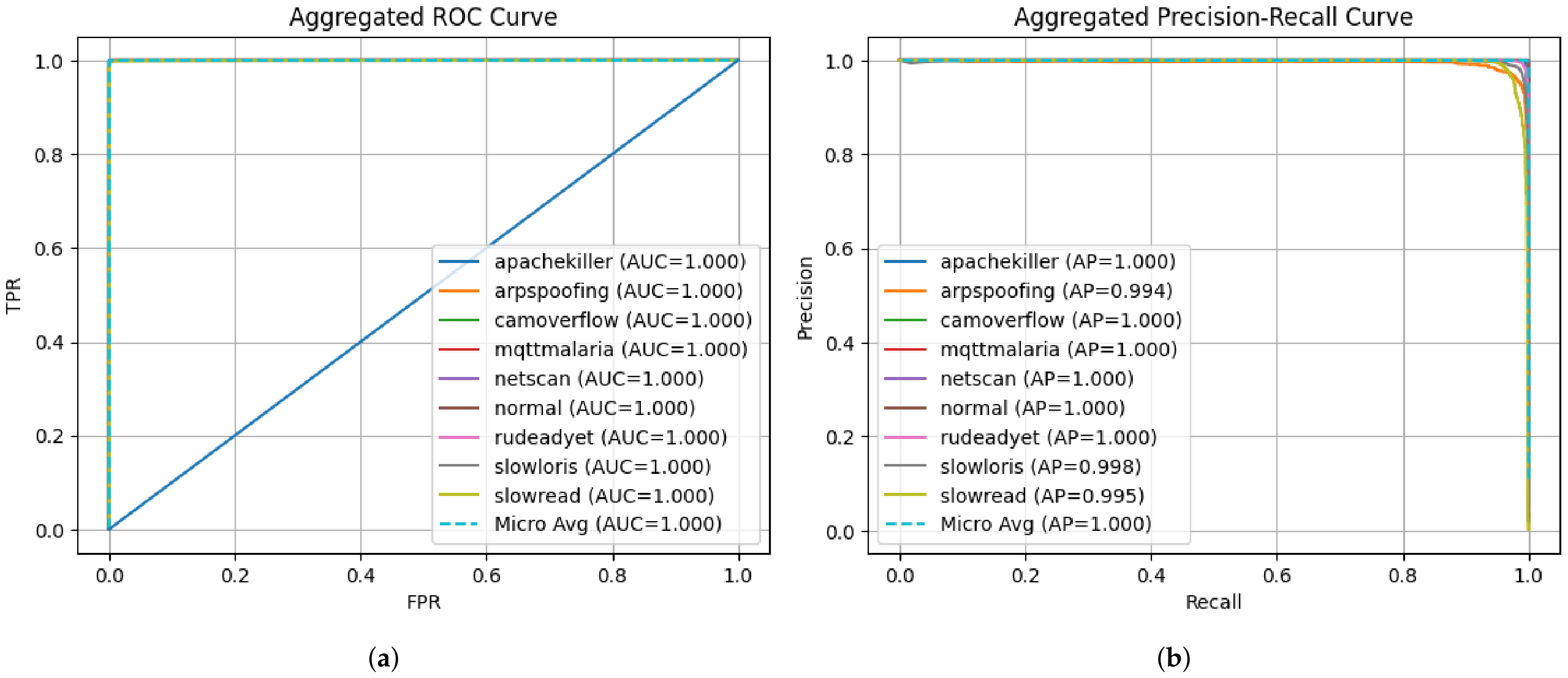
There is complete separability among assault types, as shown by the ROC curves in Figure 28a that attain an AUC of 1.000 for all classes for the CNN model on the IoMT_TrafficData. In the same way, the precision–recall curves given in Figure 28b, show that the AP values are mostly close to 1.000, with a few exceptions like 0.994 for arpspoofing and 0.995 for slowread. The micro-average AP is also 1.000. Thus, the CNN model exhibits exceptional stability and consistency on the IoMT dataset, resulting in near-perfect classification performance.

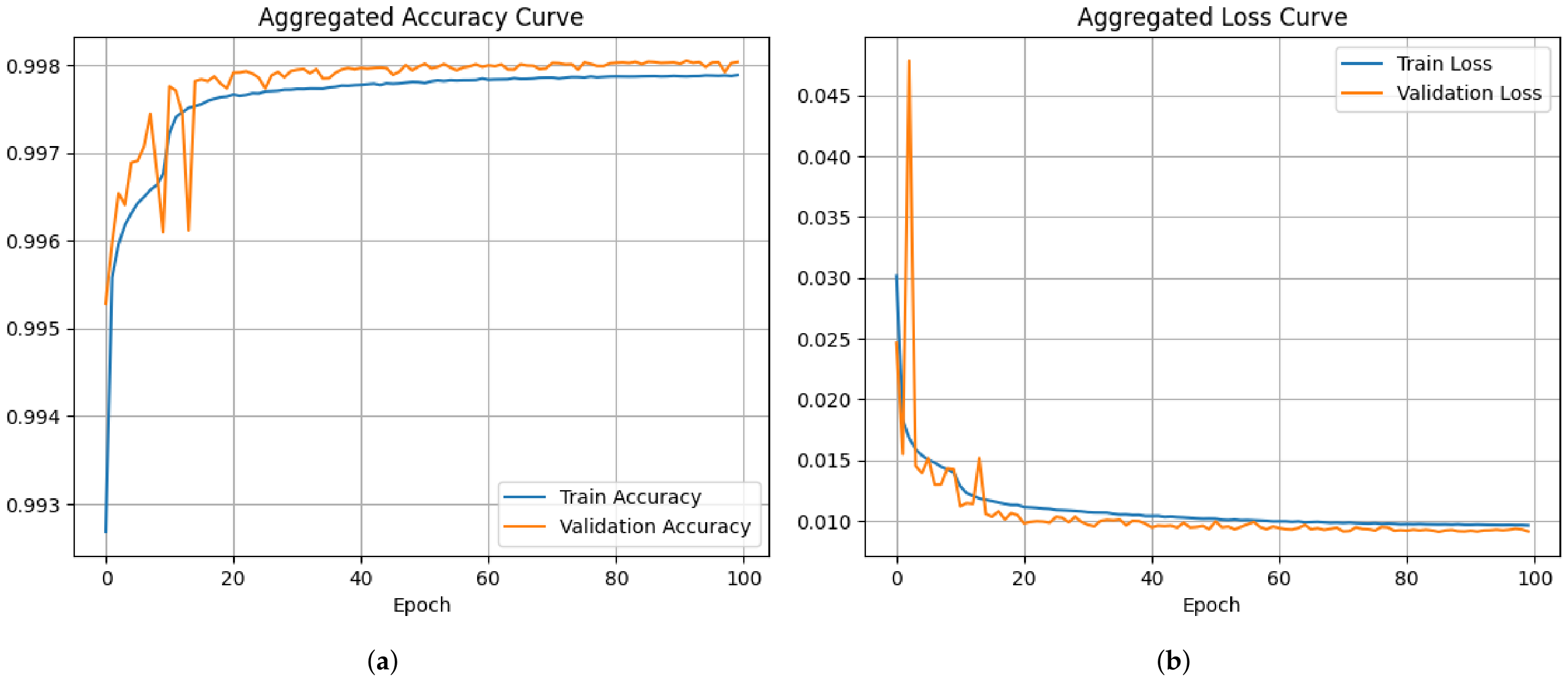
The performance of the encoder–transformer model on the IoMT-TrafficData dataset is given in Figure 29 and Figure 30. Figure 29a, shows that the combined accuracy curves for training and validation both rise sharply in the first few epochs before leveling out at roughly 99.7–99.8%. This suggests that there was quick convergence, robust generalization, and little overfitting, since the two curves matched up so closely. The aggregated loss curve, shown in Figure 29b, confirms effective learning without divergence by showing a sharp initial decline in training and validation loss followed by a progressive convergence to a very low value of nearly 0.009.

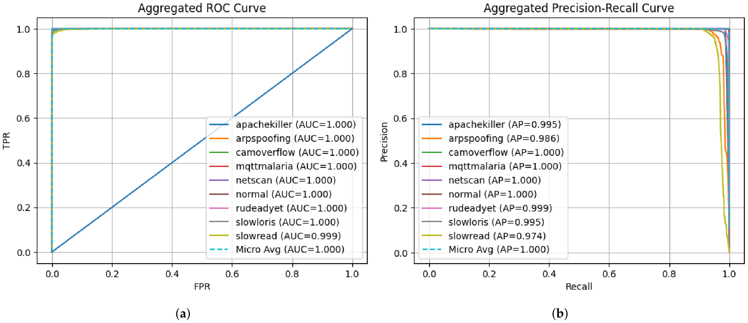
The encoder–transformer model exhibits exceptional performance across all classes with only minor variations. Almost every class on the ROC curve, as shown in Figure 30a, including apachekiller, arpspoofing, camoverflow, mqttmalaria, netscan, normal, rudeadyet, and slowloris, achieves a perfect AUC of 1.000, with the exception of slowread, which has a slightly lower AUC of 0.999, making it the only considerably weaker class while still very accurate. With perfect AP values of 1.000, the classes with the best performance on the precision–recall curve given in Figure 30b are mqttmalaria, netscan, and normal. Rudeadyet, having an AP of 0.999, and slowloris (0.995) come in a close second and third, respectively. However, apachekiller (0.995) and arpspoofing (0.986) perform somewhat worse, and slowread (0.974) is once more the class with the worst precision-recall balance. Slowread is tougher to classify, although mqttmalaria, netscan, and normal are most reliably predicted.

XAI for IoMT_TrafficData

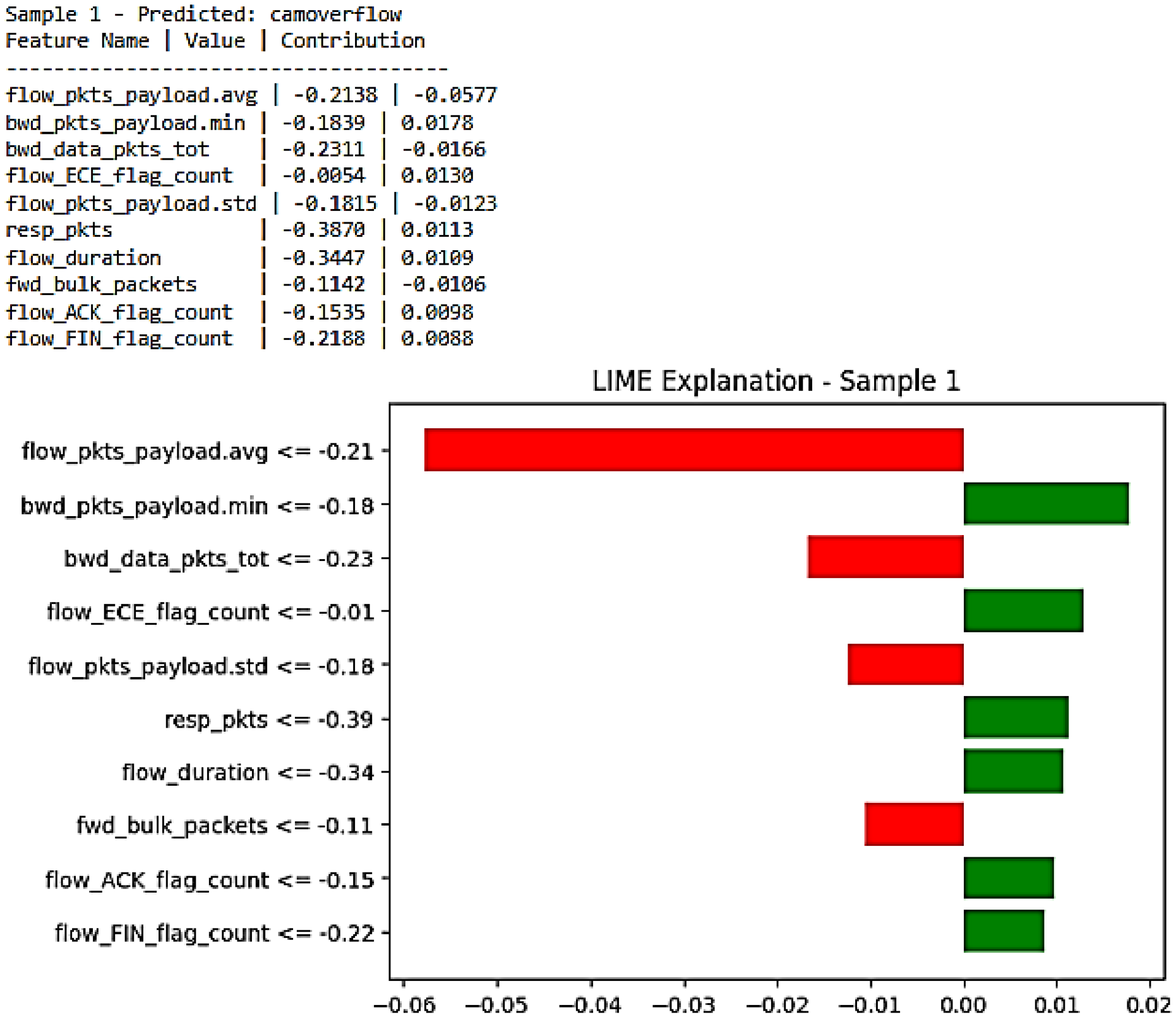
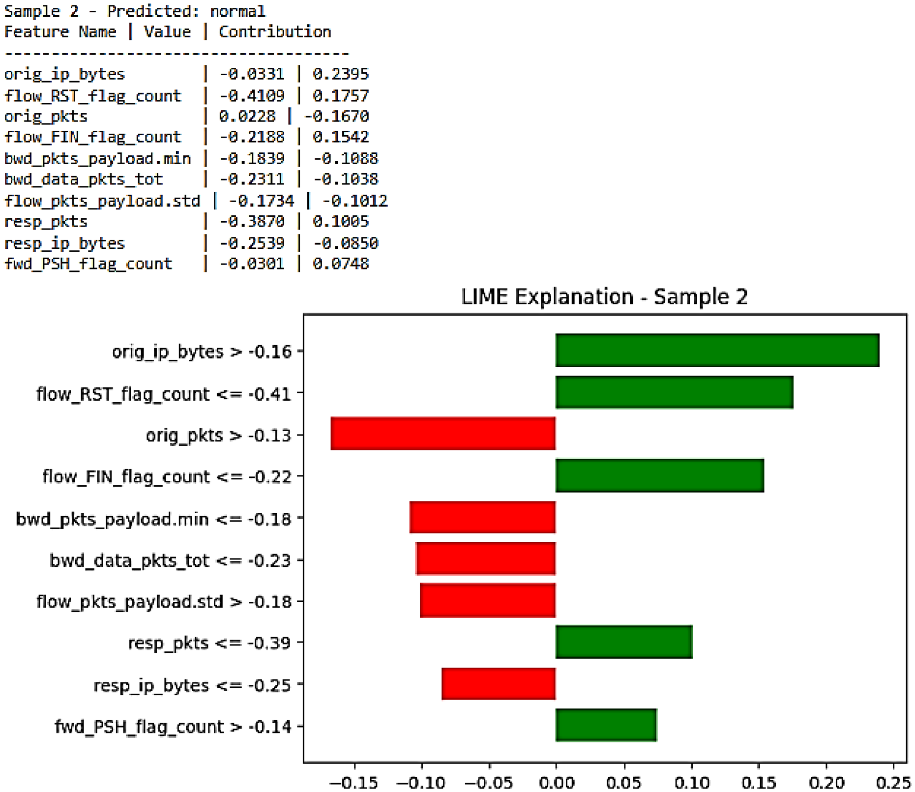
Figure 31, Figure 32 and Figure 33 show LIME explanations for DNN predictions for three samples 0, 1, and 2, respectively. They show how each feature affects the decision. Some features, like fwd_bulk_packets and resp_pkts, contribute positively, i.e., support the prediction, while others, like flow_pkts_payload.avg and flow_iat.tot, contribute negatively, i.e., oppose the prediction. The green bars represent features that move the model closer to the camoverflow class, while the red bars represent features that move it further away from the camoverflow class, as given in Figure 31 and Figure 32. Overall, the prediction is made as camoverflow because the positive features outweigh the negative ones. For Figure 33, the predicted class is normal due to positive contributions from features such as orig_ip_bytes, flow_RST_flag_count, and flow_FIN_flag_count, which outweigh the negative influence of other network traffic features.

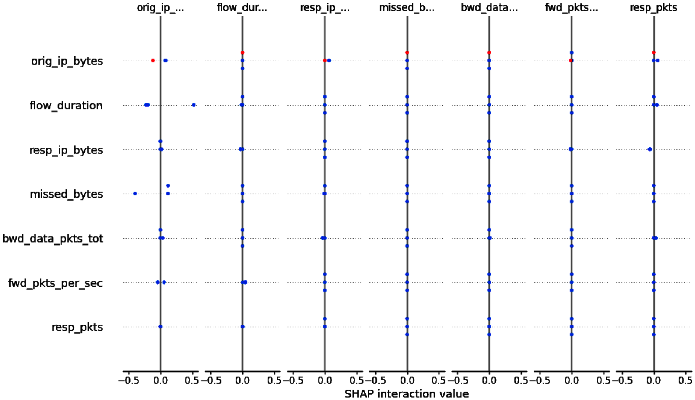
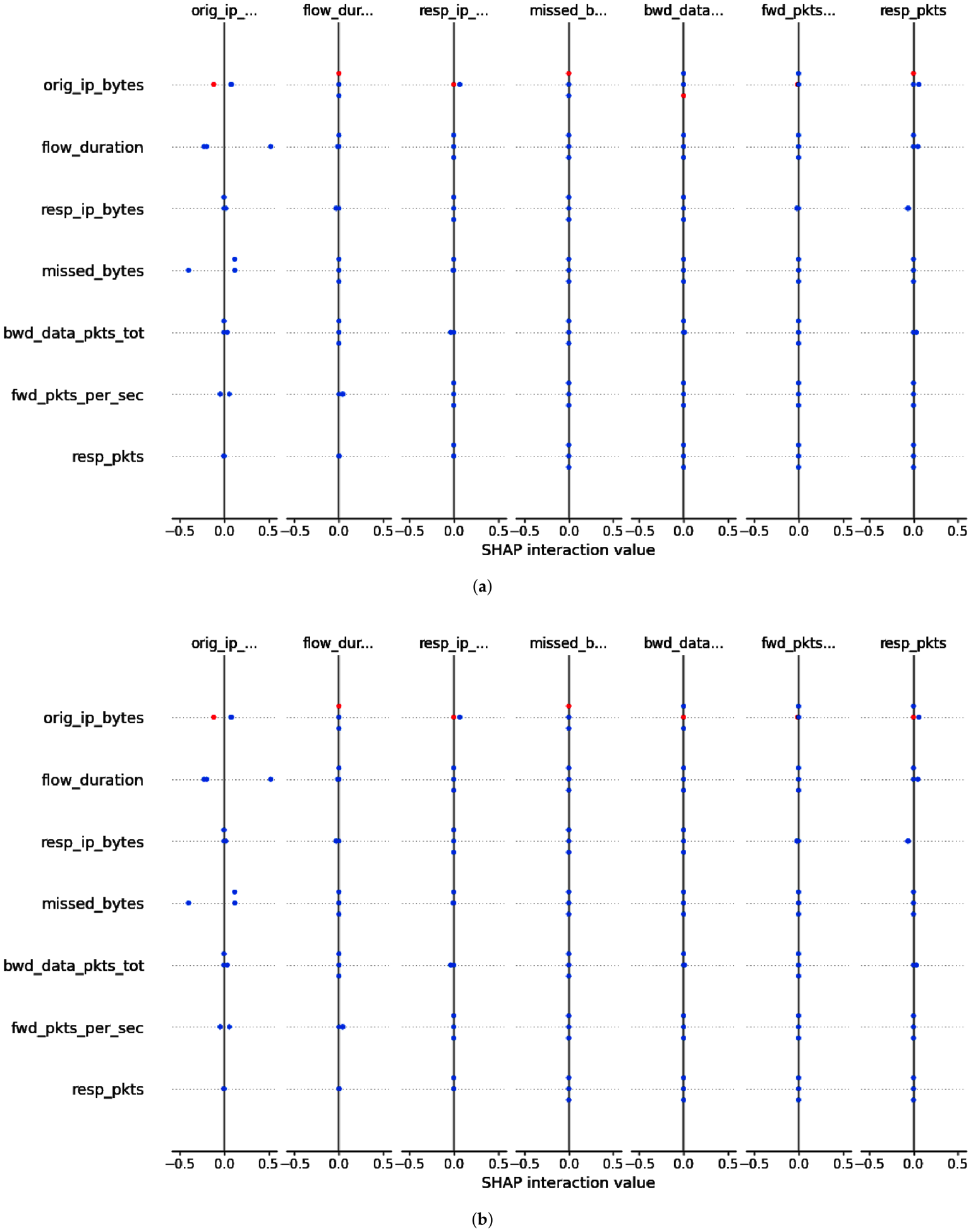
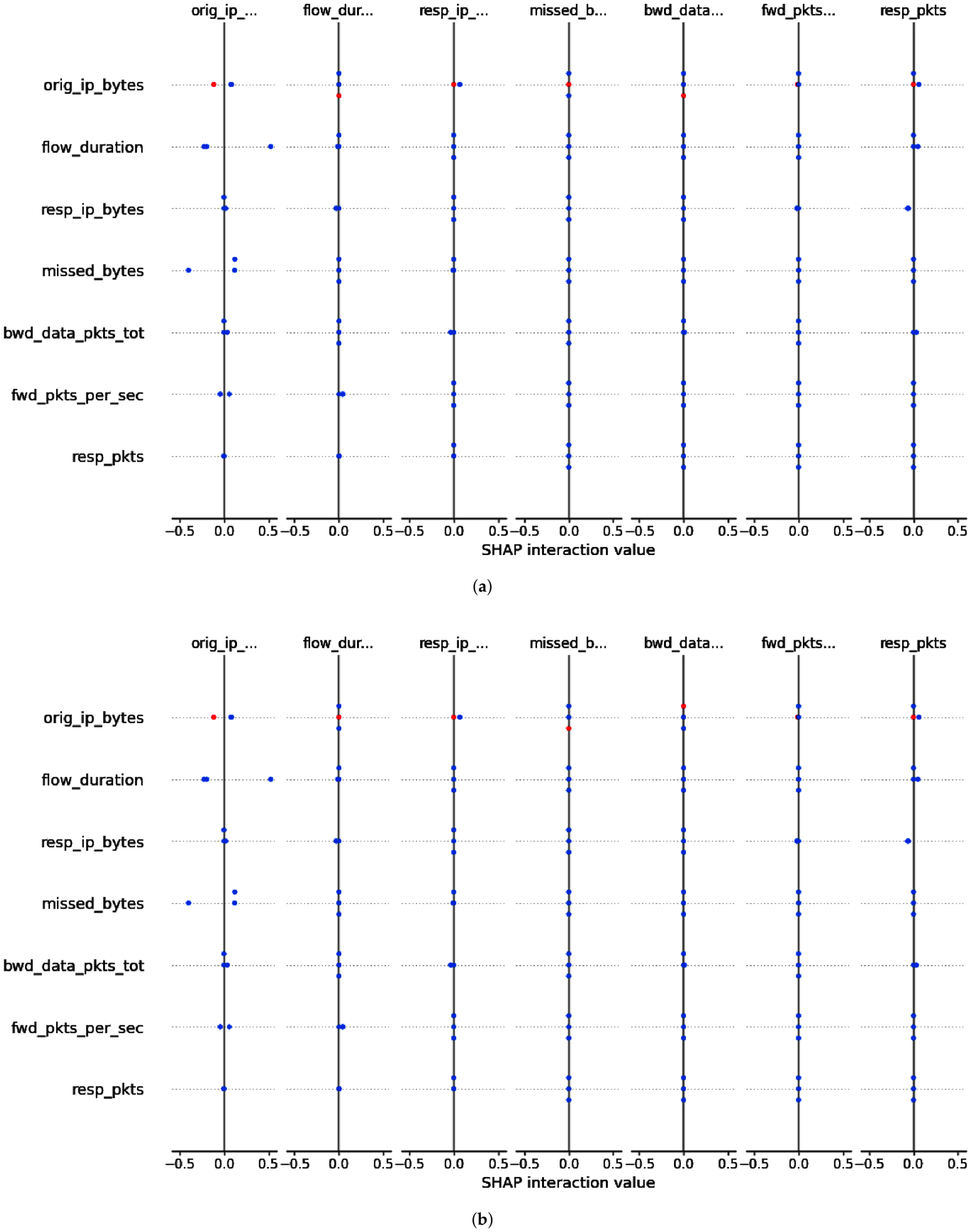
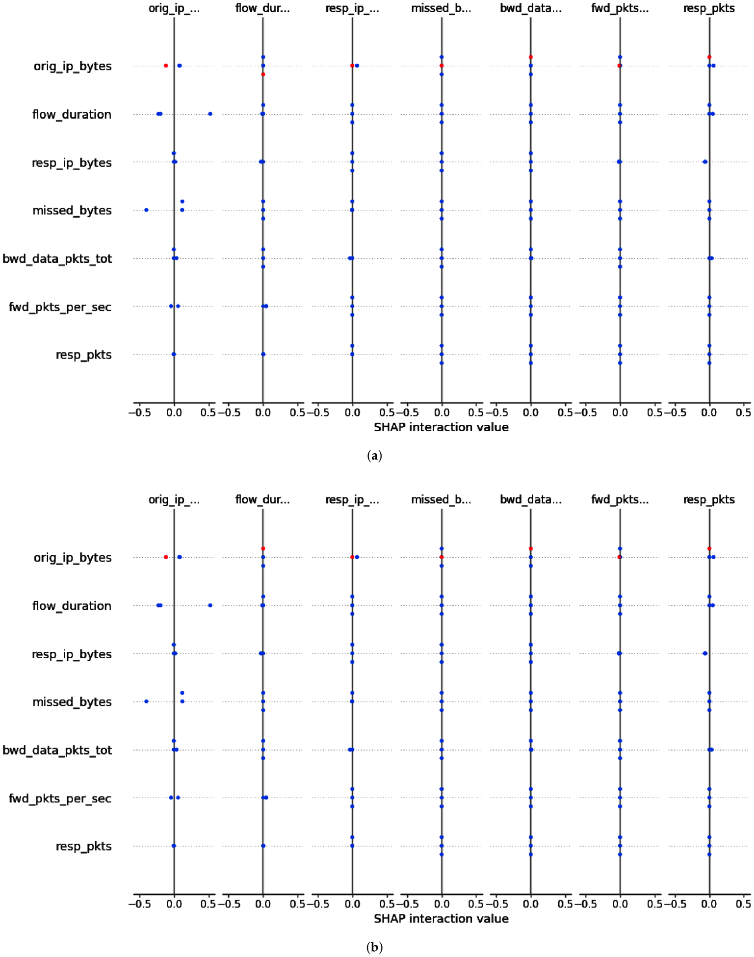
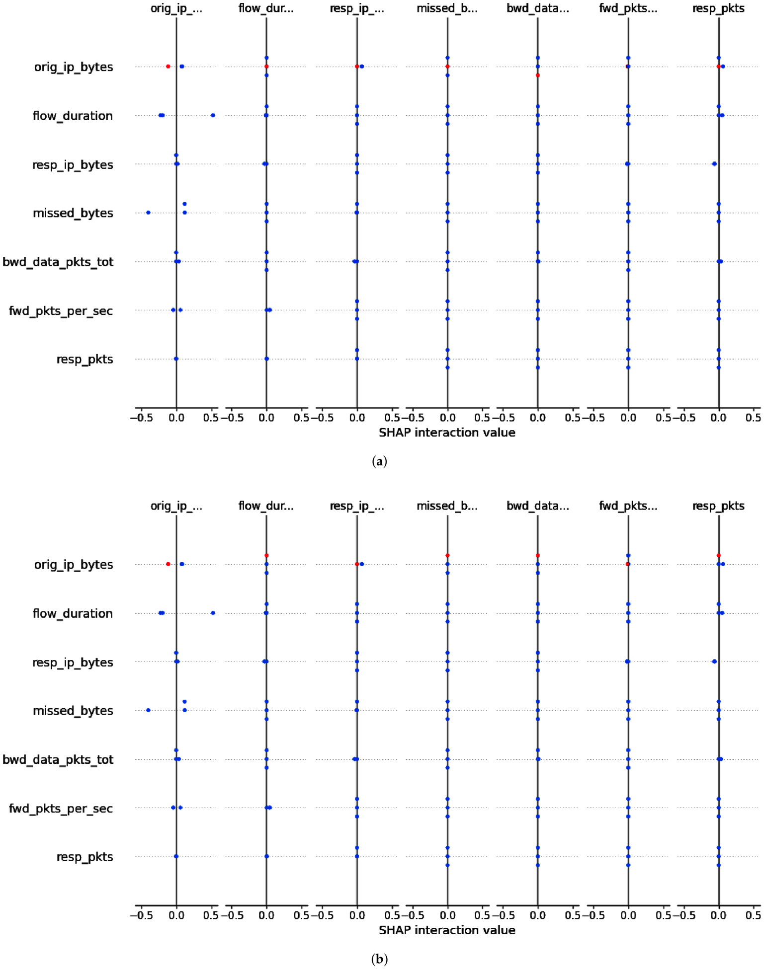
The SHAP interaction plots for a DNN model on IoMT_TrafficData for apachekiller is shown in Figure 34a, arpspoofing is shown in Figure 34b, camoverflow is shown in Figure 35a, mqttmalaria is shown in Figure 35b, netscan is shown in Figure 36a, normal is shown in Figure 36b, rudeadyet is shown in Figure 37a, slowloris is shown in Figure 37b, and slowread is shown in Figure 38, demonstrating how each network feature contributes to the model’s predictions and interacts with one another. The horizontal axis in all subplots indicates the SHAP interaction value, while each vertical strip refers to a characteristic such as orig_ip_bytes, flow_duration, resp_ip_bytes, missed_bytes, bwd_data_pkts_total, fwd_pkts_per_sec, and resp_pkts. The plots that have points clustering around zero suggest that feature interactions are often weak. This means that the model depends more on the impact of individual features than on significant pairwise dependencies.

Moreover, Flow time, orig ip bytes, and bwd data packets are the features that are used to discriminate between different types of attacks; nevertheless, there is some evidence that these factors have a significantly larger impact than others. The resemblance of patterns among various attack types and the typical class suggests that the DNN identifies common behavioral characteristics, although minor variations in distribution assist in distinguishing unique assaults. Overall, the results show that a mixture of minor contributions from several traffic aspects allows the model to successfully categorize a variety of network behaviors, even while no particular feature interaction substantially dominates.

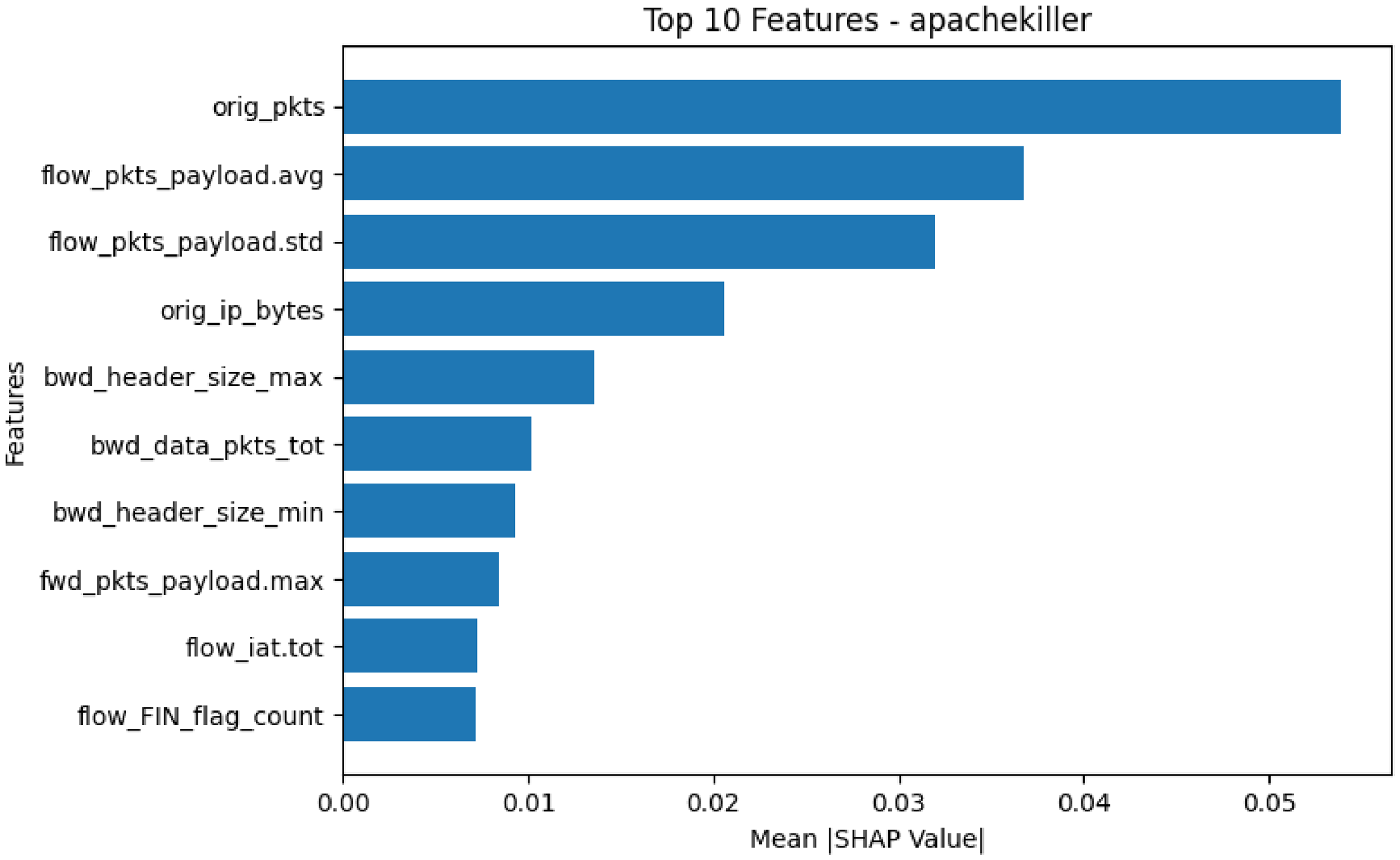
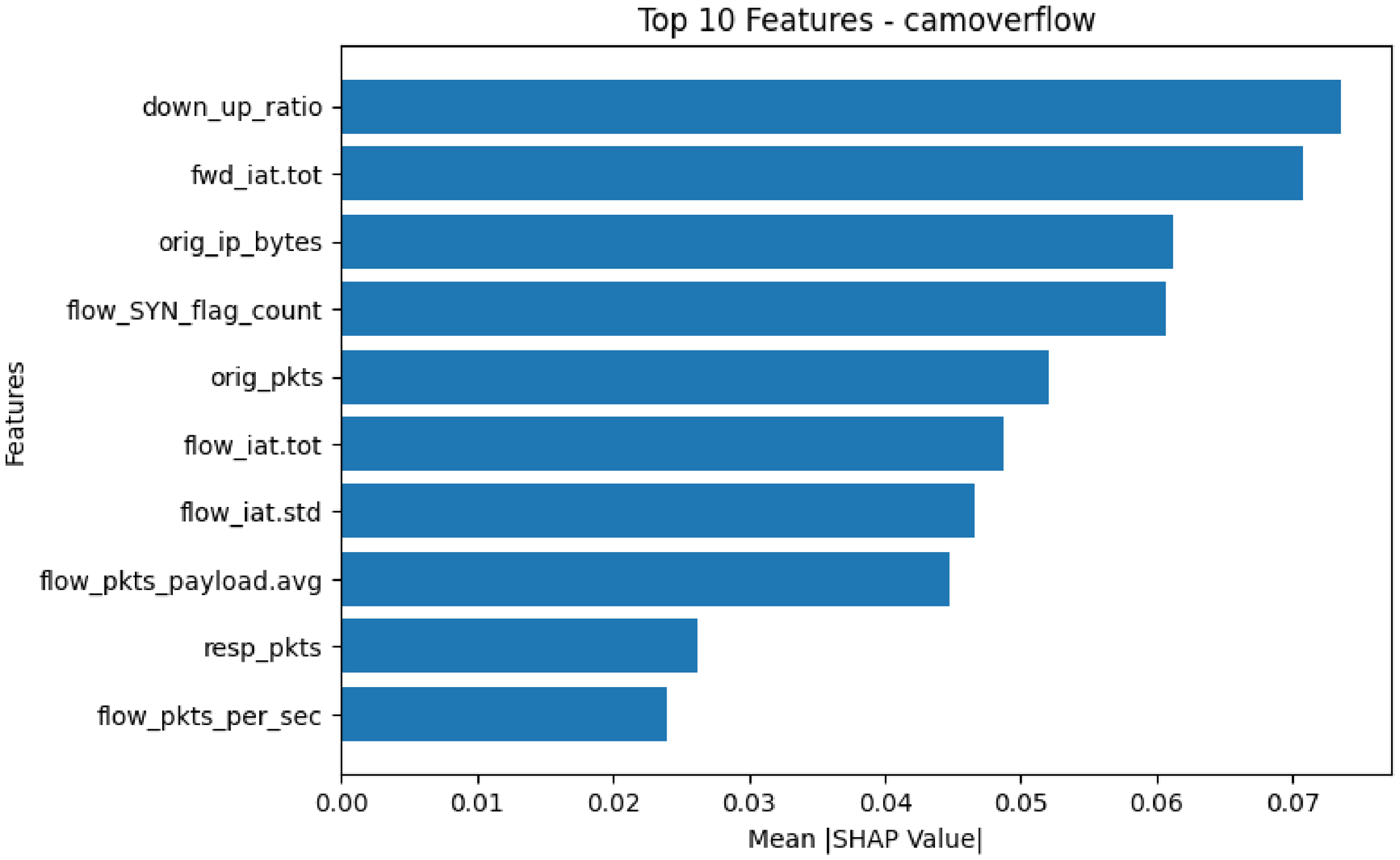
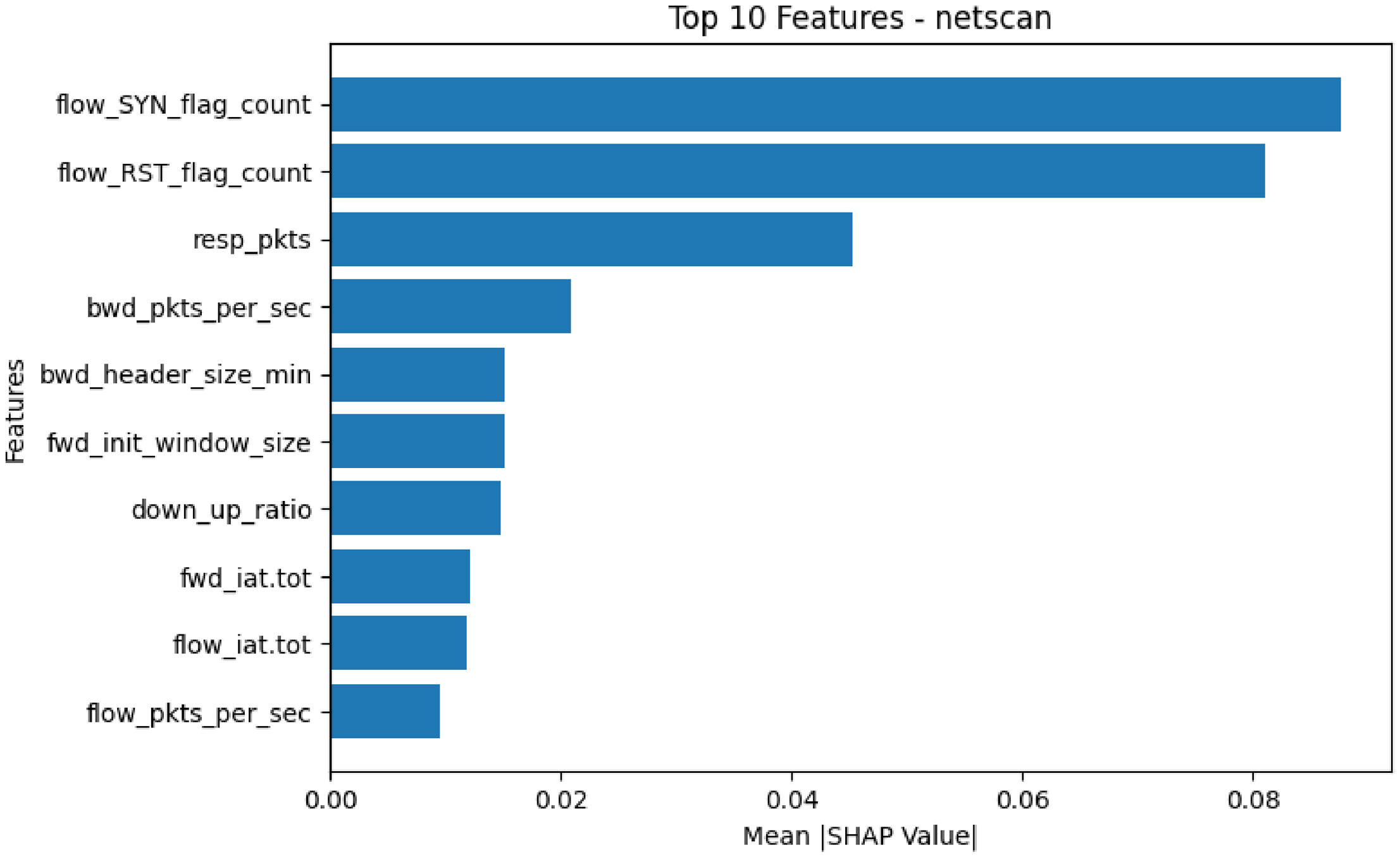
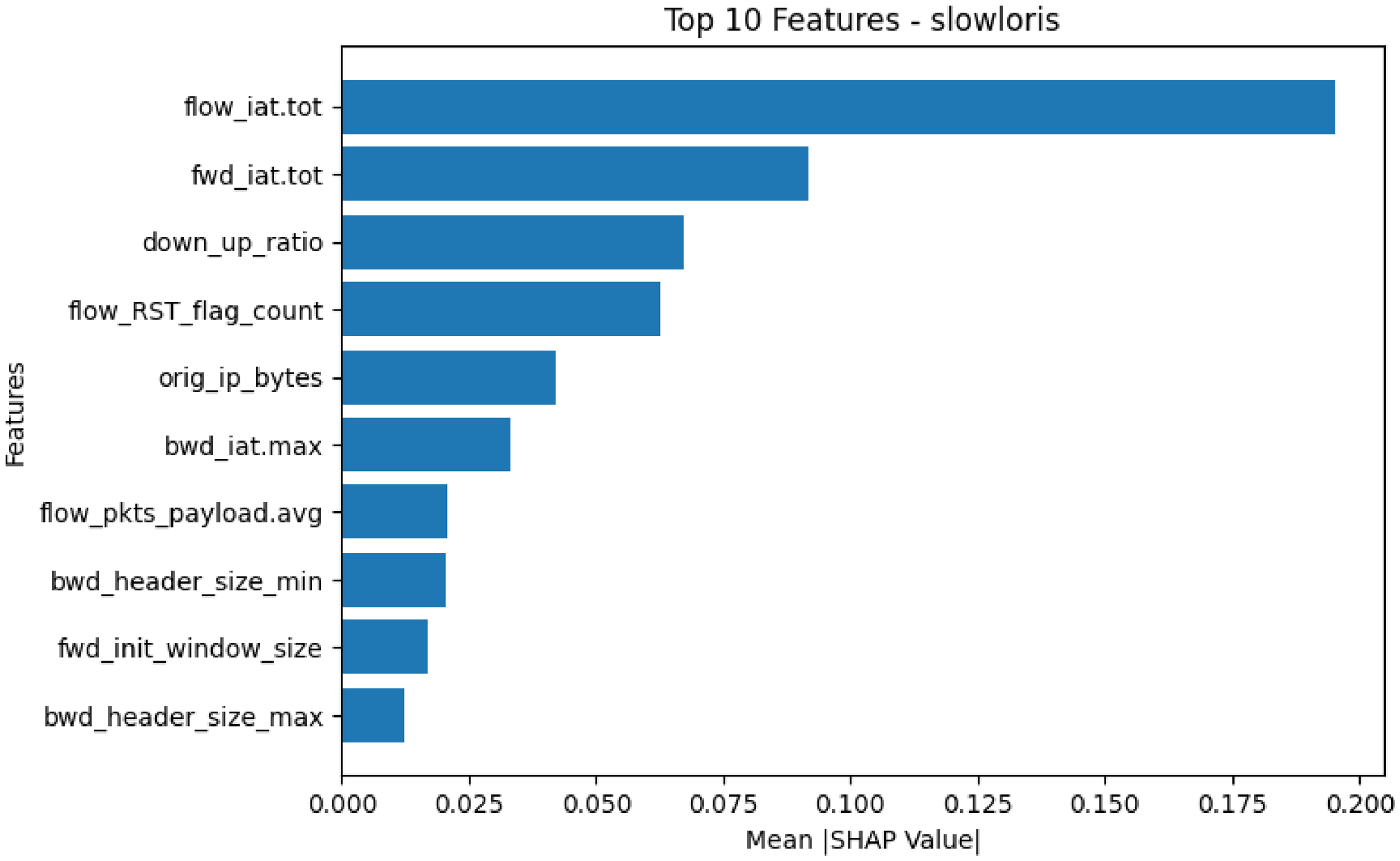
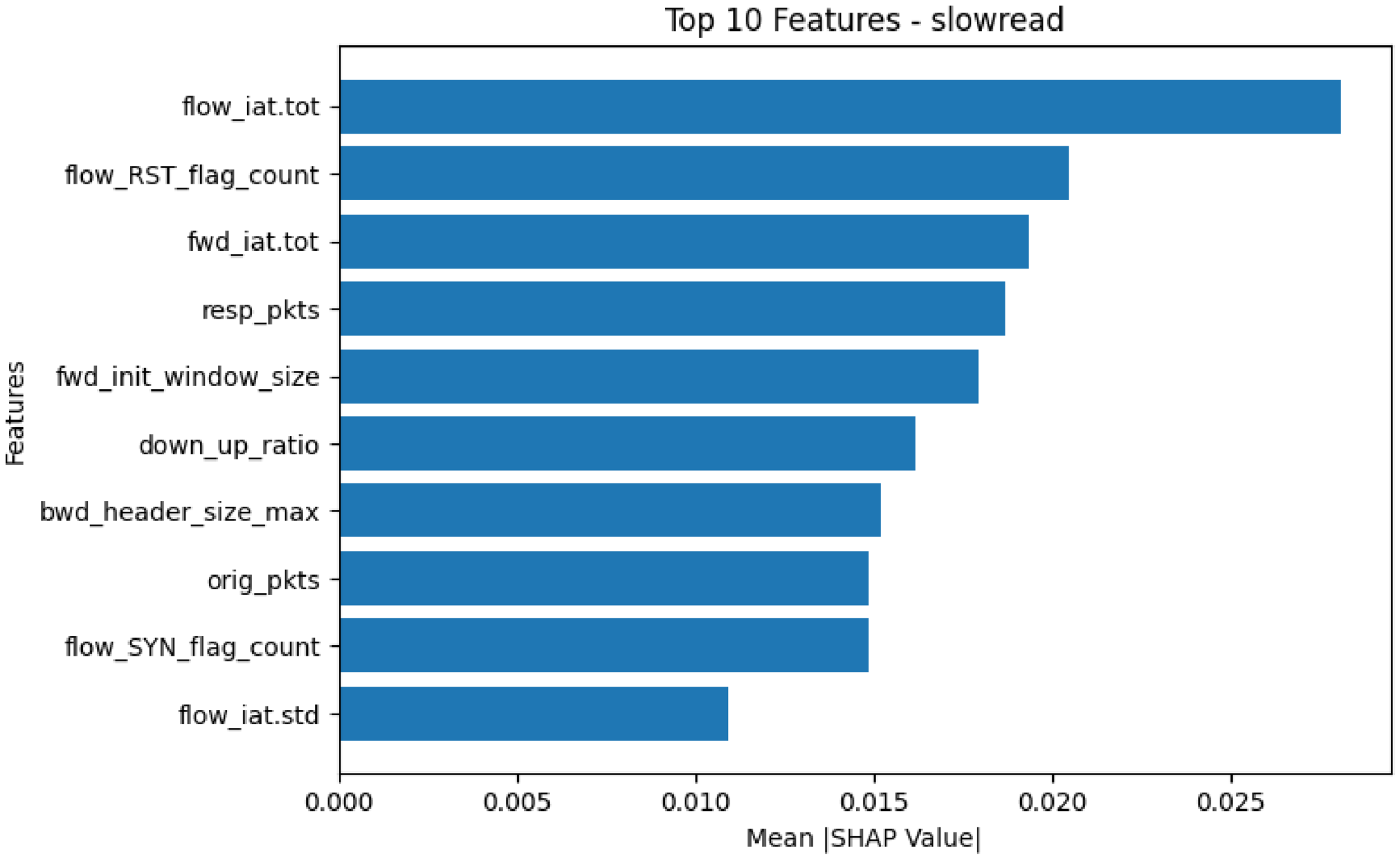
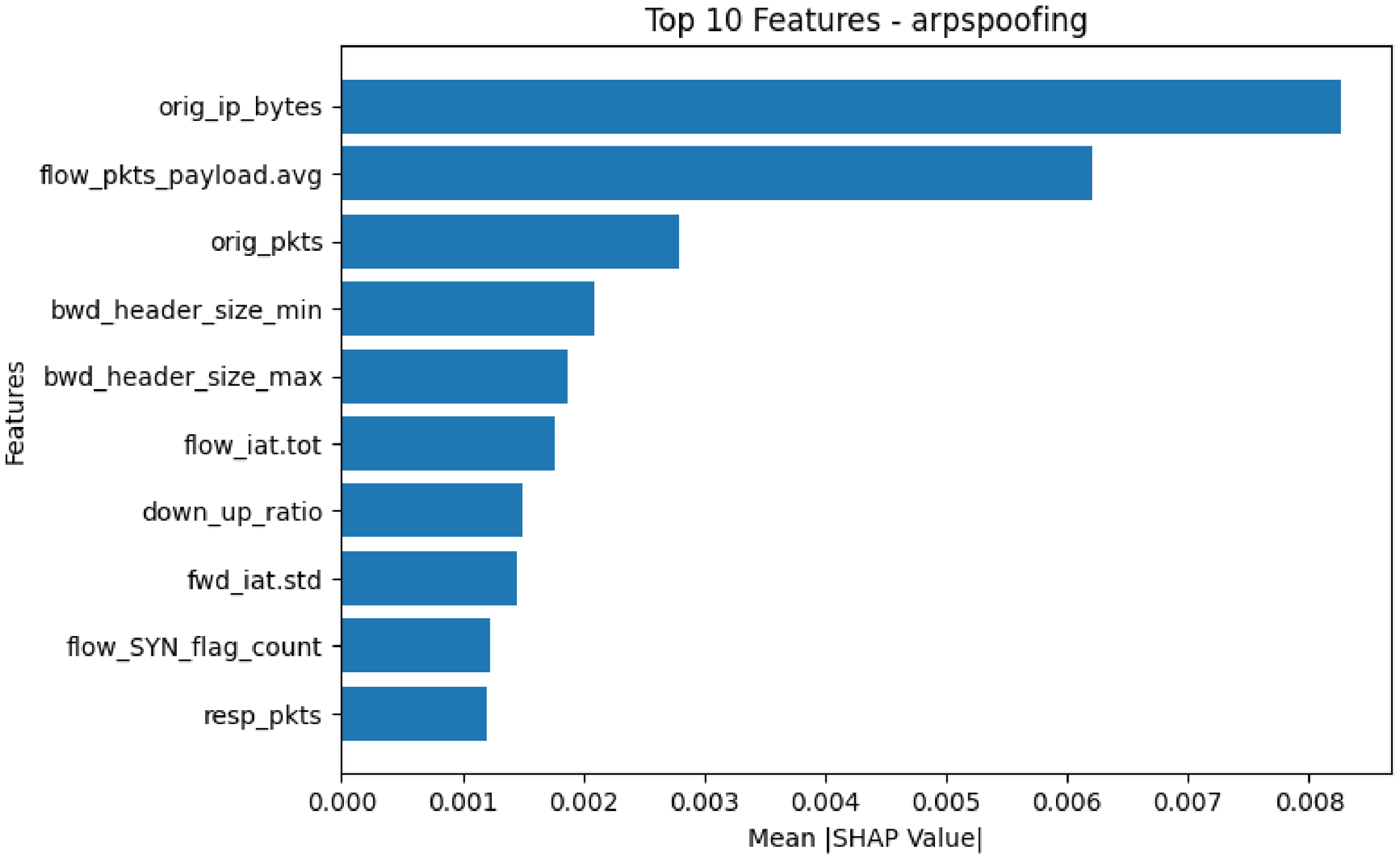
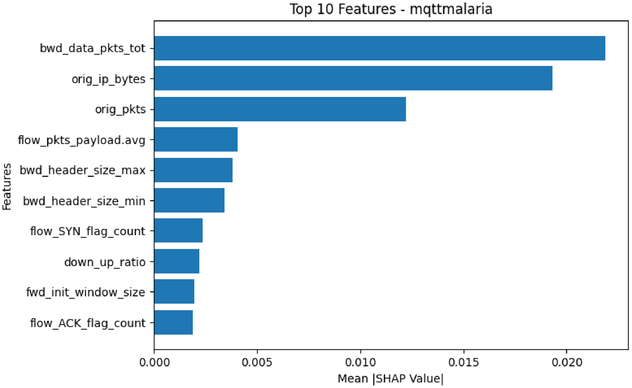
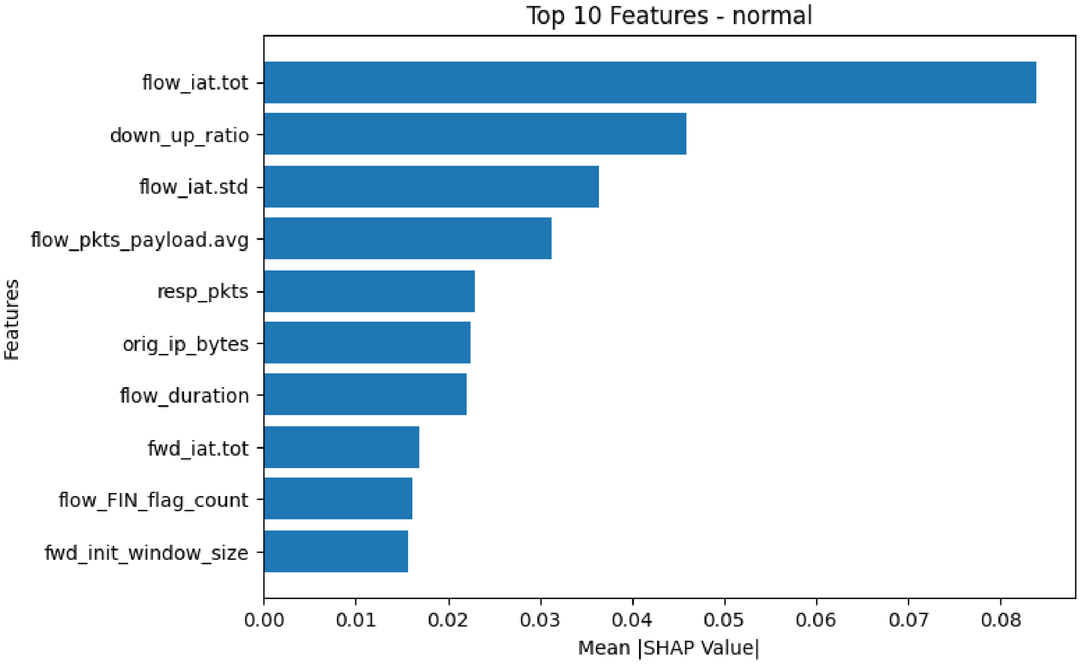
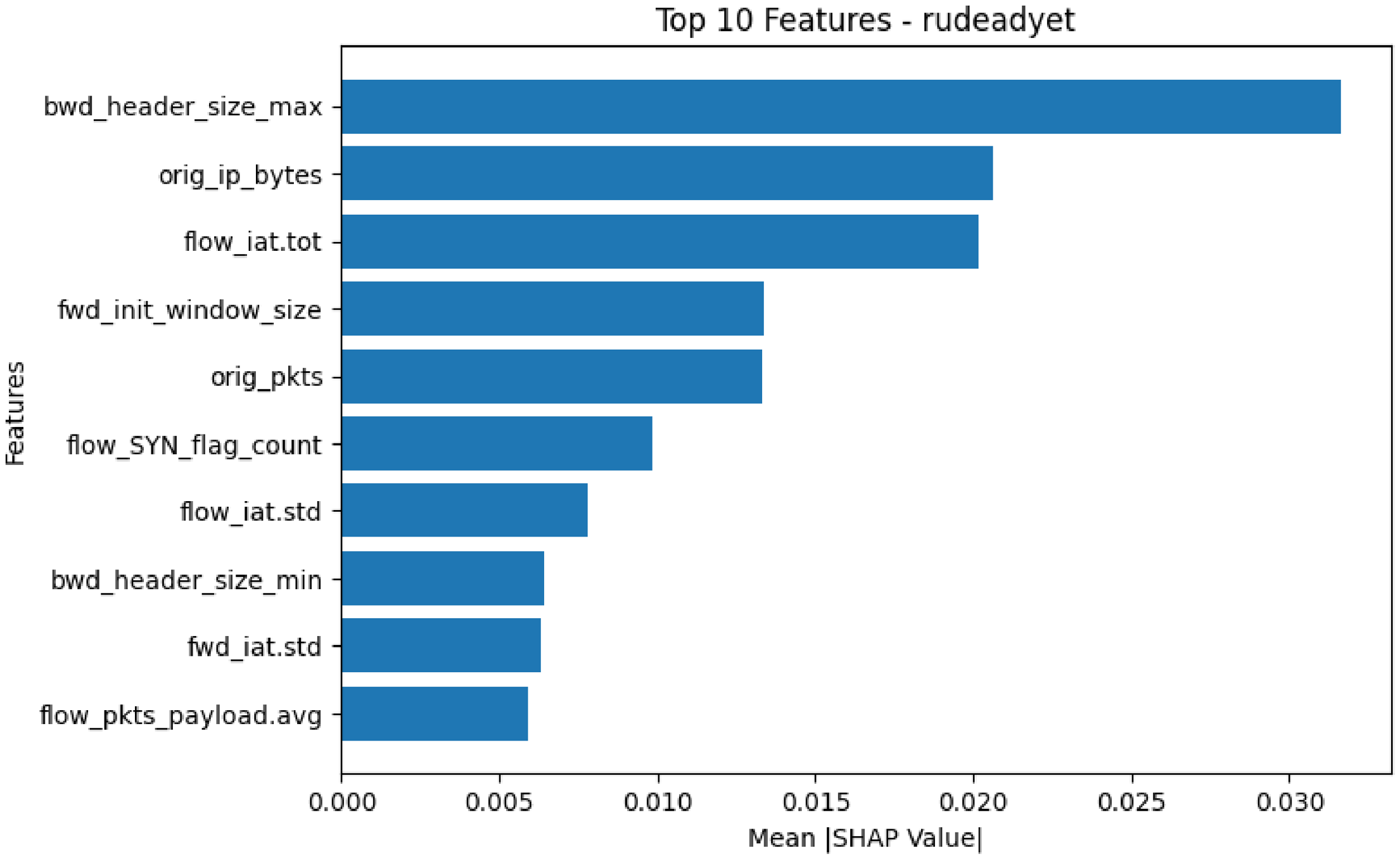
The SHAP feature importance for IoMT_TrafficData, given in Figure 39, Figure 40, Figure 41, Figure 42, Figure 43, Figure 44, Figure 45, Figure 46 and Figure 47, identifies the most significant variables that influence the classification of various attack categories and regular traffic. For apachekiller, features related to packets and payloads, like orig_pkts and flow_pkts_payload.avg, are the most important as given in Figure 39. On the other hand, orig_ip_bytes and payload statistics are the important features that define arpspoofing as given in Figure 40. The camoverflow class is significantly impacted by traffic direction and timing features, specifically down_up_ratio and fwd_iat.tot as given in Figure 41. In mqttmalaria, bwd_data_pkts_tot, orig_ip_bytes, and orig_pkts are the primary contributors to the detection of an attack as given in Figure 22. The netscan attack can be identified by TCP flag-based characteristics, notably flow_SYN_flag_count and flow_RST_flag_count, which show that the attack probes connections in depth as given in Figure 43. The most significant features for rudeadyet are those that pertain to headers and traffic volume, including bwd_header_size_max and orig_ip_bytes as given in Figure 44. Inter-arrival time metrics like flow_iat.tot and fwd_iat.tot are the main contributors for the detection of slowloris and slowread attacks, as given in Figure 45 and Figure 46, because they show how slowly they communicate. Finally, steady timing and flow characteristics like flow_iat.tot, down_up_ratio, and flow_iat.std characterize normal traffic as given in Figure 47. In general, the findings indicate that the most important distinguishing factors of attack classes and benign network traffic are the packet volume, payload characteristics, TCP flags, header information, and temporal flow statistics. These characteristics are the essential discriminative aspects that enable successful distinction.

4.3. Robustness Evaluation Under FGSM and PGD Adversarial Attacks

The robustness evaluation of the DNN model on the CICIoMT and IoMT datasets under FGSM and PGD adversarial attacks is presented in

Table 4. Robustness analysis of the DNN model under FGSM and PGD adversarial attacks on CICIoMT and IoMT datasets.

Dataset	Fold	FGSM Acc. (%)	FGSM Drop (%)	PGD Acc. (%)	PGD Drop (%)	OOD Rate (%)
DNN_IoMT	1	87.15	12.72	99.75	0.12	0.28
	2	91.02	8.86	99.45	0.43	0.29
	3	95.35	4.52	99.72	0.15	0.33
	4	92.92	6.96	99.55	0.33	0.32
	5	95.69	4.19	99.59	0.29	0.32
	Mean ± Std	92.43 ± 3.14	7.45 ± 3.14	99.61 ± 0.11	0.26 ± 0.11	0.31 ± 0.02
	95% CI	[88.53, 96.33]	[3.55, 11.35]	[99.47, 99.75]	[0.12, 0.40]	[0.28, 0.34]
DNN_CICIoMT	1	99.52	0.09	99.52	0.08	0.95
	2	99.42	0.15	99.43	0.14	0.96
	3	99.46	0.14	99.47	0.13	0.89
	4	99.51	0.08	99.51	0.08	0.94
	5	99.36	0.31	99.36	0.31	0.93
	Mean ± Std	99.45 ± 0.06	0.15 ± 0.08	99.46 ± 0.06	0.15 ± 0.09	0.94 ± 0.02
	95% CI	[99.38, 99.52]	[0.05, 0.25]	[99.39, 99.53]	[0.04, 0.26]	[0.91, 0.97]

, and was conducted using five-fold cross-validation. The results show that the DNN model on the CICIoMT dataset was very stable in the face of adversarial attacks, with an average FGSM Accuracy of 99.45 ± 0.06% and a PGD Accuracy of 99.46 ± 0.06%. It also had very low FGSM and PGD accuracy drops of about 0.15%.

Additionally, as the OOD detection rate is 0.94 ± 0.02%, it shows that unobserved data distributions can be consistently detected. The DNN model on the IoMT dataset, on the other hand, demonstrated a somewhat lower level of robustness against FGSM attacks. It achieved a mean FGSM Accuracy of 92.43 ± 3.14% with an FGSM drop of 7.45 ± 3.14%, which indicates a larger sensitivity to perturbation-based adversarial samples. However, the model was very strong against PGD attacks; it achieved a PGD Accuracy of 99.61 ± 0.11% with only a 0.26 ± 0.11% drop in performance. The CICIoMT dataset showed more consistent and steady resilience performance, in contrast to the IoMT dataset, which had a bigger standard deviation, suggesting greater variability among folds. Overall, the results show that, especially in situations involving recurrent PGD attacks, the suggested DNN framework has excellent adversarial resilience and dependable detection capacity across both datasets.

4.4. Statistical Analysis

The results of the five-fold cross-validation experiments for the DNN, CNN, and ET models on the CICIoMT and IoMT datasets were analyzed statistically using the Shapiro–Wilk normality test, paired t-test, and Wilcoxon signed-rank test. The results are presented in

Table 5. Statistical significance analysis using balanced accuracy and F1-score across five-fold cross-validation results.

Dataset	Metric	Comparison	Shapiro-p	t-Stat	p-Value	Wilcoxon Stat	Wilcoxon-p
CICIoMT	Balanced Accuracy	DNN vs. CNN	0.8112	5.5375	0.0052	0	0.0625
CICIoMT	Balanced Accuracy	DNN vs. ET	0.3158	2.1187	0.1015	1	0.1250
CICIoMT	Balanced Accuracy	CNN vs. ET	0.5957	−5.7401	0.0046	0	0.0625
CICIoMT	F1-score	DNN vs. CNN	0.5257	5.7828	0.0044	0	0.0625
CICIoMT	F1-score	DNN vs. ET	0.2840	2.6490	0.0570	0	0.0625
CICIoMT	F1-score	CNN vs. ET	0.7033	−5.8022	0.0044	0	0.0625
IoMT	Balanced Accuracy	DNN vs. CNN	0.0004	−0.9457	0.3978	7	1.0000
IoMT	Balanced Accuracy	DNN vs. ET	0.0005	−0.6476	0.5525	5	0.6250
IoMT	Balanced Accuracy	CNN vs. ET	0.4221	6.2759	0.0033	0	0.0625
IoMT	F1-score	DNN vs. CNN	0.0002	−1.0381	0.3578	1	0.1250
IoMT	F1-score	DNN vs. ET	0.0003	−0.8408	0.4478	5	0.6250
IoMT	F1-score	CNN vs. ET	0.8989	21.3542	2.84 × 10−5	0	0.0625

. On the CICIoMT dataset, the DNN model did much better than the CNN model in terms of balanced accuracy ($p=0.0052$) and F1-score ($p=0.0044$). The ET model also performed better than CNN, with p-values of $0.0046$ and $0.0044$, respectively. Balanced accuracy ($p=0.1015$) and F1-score ($p=0.0570$) showed no statistically significant variations in performance between DNN and ET, suggesting that the two models performed similarly. There were no statistically significant changes between DNN and CNN or between DNN and ET in the IoMT dataset, as all of the p-values were higher than 0.05. In contrast, CNN demonstrated a substantial improvement over ET in both the F1-score ($p=2.84\times {10}^{-5}$) and balanced accuracy ($p=0.0033$). The Shapiro–Wilk results show that a number of IoMT comparisons did not follow the normality assumption, which supports the use of both parametric and non-parametric statistics tests. Hence, the statistical analysis shows that the DNN model can reliably and effectively classify both the CICIoMT and IoMT datasets. Additionally, the DNN model outperforms the CNN model on the CICIoMT dataset by a substantial margin, while both models demonstrate statistically equivalent performance on the IoMT dataset.

5. Discussion

The DNN model consistently outperforms both CNN and ET throughout the CICIoMT2024 and IoMT_TrafficData datasets. In CICIoMT2024, the DNN achieves near-perfect performance, with an average accuracy of roughly 99.65% during cross-validation and 99.68% on the test set, greatly outperforming CNN’s 76.78% accuracy. Similar to this, all models perform well in IoMT_TrafficData since the dataset is more clearly separable, although the DNN still has a tiny advantage with an accuracy of 99.87% and an F1-score of 98.99%. These findings suggest that the DNN is more effective in capturing complex, non-linear relationships within network traffic than the CNN and ET, while still maintaining a reasonable level of computational efficiency.

The proposed method outperforms other methods as given in

Table 6. Performance comparison of existing methods and the proposed model on IoMT datasets.

Research	Dataset	Method	Accuracy (%)	AUC
Hafid et al. [14]	CICIoMT2024	XGBoost + SHAP	97	–
Torre et al. [23]	CICIoMT2024	CNN	97.31	–
Rehaman et al. [24]	CICIoMT2024	IG, MI, Fisher Score + ML	97.7	–
	IoMT_TrafficData		98.7	–
Akar et al. [25]	CICIoMT2024	LSTM	98	–
Bo et al. [26]	CICIoMT2024	Meta-learning + Feature Fusion	97.78	–
Palaniappan et al. [27]	CICIoMT2024	ProxyNet + MI Filtering + ML	–	0.9998
	IoMT_TrafficData		–	0.9997
Proposed	CICIoMT2024	PSO + Deep Learning + XAI (5-fold CV)	$99.68$	$0.9999$
	IoMT		$99.87$	$0.9999$

, which provides a comparative assessment of various intrusion detection methods across the CICIoMT2024 and IoMT_TrafficData datasets, emphasizing their accuracy and AUC performance. Existing approaches, like XGBoost with SHAP, CNN, LSTM, and meta-learning-based feature fusion, obtain accuracy rates ranging from about 97% to 98%, indicating robust but somewhat restricted detection power.

As per the LIME and SHAP analysis, the CICIoMT2024 dataset is strongly reliant on connection-level parameters, including length, protocol type, and TCP flag-based features. Benign traffic is distinguished by its balanced feature contributions, which show consistent communication patterns. High SYN flag numbers and short durations, which indicate flooding behavior, are the primary drivers of DDoS and DoS attacks, respectively; DDoS displays more severe patterns. The kind of protocol significantly affects MQTT traffic, validating that the model accurately captures protocol-specific properties. Spoofing attacks are separated from recon attacks by discrepancies between SYN and ACK flags, which indicate anomalous communication behavior. Short durations and frequent state changes characterize recon assaults. In the IoMT Traffic dataset, packet, payload, TCP flag, and flow time features are paramount, whereas IAT, ack_flag_number, number of packets, and variance predominate in CICIoMT2024. These results are consistent for LIME and SHAP analysis and provide further evidence that the selected characteristics provide a high degree of discriminative power, which is necessary for accurate IoMT attack detection.

Similarly, the IoMT_TrafficData dataset indicates a more dispersed pattern of feature relevance, with no single feature predominating across all attack types. Instead, flow-based parameters, including flow length, original and response byte counts, and packet speeds, are important factors. For instance, apachekiller and slowloris attacks are linked to long-lived connections and lengthy flow durations, whereas arpspoofing and netscan attacks are linked to high packet rates and short-lived flows. Attacks such as camoverflow and rudeadyet are associated with anomalous payload sizes and byte distributions, whereas mqttmalaria represents irregular IoT communication bursts. Normal traffic, by contrast, has balanced contributions across features, indicating stable and consistent activity. This shows that the model adjusts to varied IoMT traffic patterns using complementary features.

Despite its high performance, this research has some limitations, such as SHAP being computationally expensive. It may not scale well for large or real-time systems, despite its usefulness for interpretability. Additionally, it fails to account for sequential patterns or temporal dependencies in network traffic. Furthermore, adversarial scenarios are not considered because the datasets used are open-source, which may have an effect on the resilience of the model when it is successfully deployed in the real world.

6. Conclusions

The paper proposes a novel hybrid framework, DeepMedShield-XAI, that uses a metaheuristic algorithm for feature selection and then uses the selected features for training the CNN, DNN, and encoder–transformer models. The proposed framework has three major steps. The first step is to pre-process the dataset and use the PSO algorithm for feature selection. The second step is to train three DL models, i.e., DNN, CNN, and the encoder–transformer model, using the selected features. The third step is to analyze the predictions made by the models using explainable artificial intelligence (XAI) methods. Local analysis of a particular sample is performed to find the features responsible for the prediction. On the other hand, global analysis is also performed to find the common features responsible for classifying a particular sample into a particular class. For each class, a separate SHAP analysis is shown by highlighting the features that affect it positively and negatively. The highest performance is achieved by the PSO and DNN hybrid model, which attains accuracies of 99.68% and 99.87% on CICIoMT2024 and IoMT_TrafficData. Despite the optimistic performance, the research has the potential to be expanded in the future to incorporate real-time datasets for adversarial attacks and computationally efficient XAI methods, which can potentially result in low computational saturation.

References

1. Munshar, H.H.A.; Jemili, F.; Korbaa, O.; Alauthmaan, M. Comprehensive analysis of intrusion detection systems for enhancing security in internet of things environments. Discov. Appl. Sci. 2026, 8, 473. [Google Scholar] [CrossRef] [Scilit]
2. Ogunseyi, T.B.; Thiyagarajan, G.; He, H.; Bist, V.; Du, Z. Performance Analysis of Explainable Deep Learning-Based Intrusion Detection Systems for IoT Networks: A Systematic Review. Sensors 2026, 26, 363. [Google Scholar] [CrossRef] [Scilit] [PubMed]
3. Raychaudhuri, A.; Dutt, I. Intrusion Detection in Cloud-IoT Systems: Challenges and Opportunities. In Strategic Approaches to Intrusion Detection in Cloud-IoT Ecosystem; John Wiley & Sons: Hoboken, NJ, USA, 2026; pp. 1–30. [Google Scholar]
4. Alqahtani, A.; Abdullah, M. A Review on Intrusion Detection Models in Internet of Medical Things (IoMT). Int. J. Adv. Comput. Sci. Appl. 2026, 17, 361. [Google Scholar] [CrossRef] [Scilit]
5. Hazman, C.; Douiba, M.; Guezzaz, A.; Ravi, V.; Azrour, M.; Benkirane, S. Intrusion Detection Approaches in Healthcare Systems: An Overview. In Reliability in Cyber-Physical Systems: The Human Factor Perspective; Springer: Berlin/Heidelberg, Germany, 2026; pp. 131–145. [Google Scholar]
6. Ramya, M.; Sudhakaran, P.; Sivagnanam, Y.; Krishnan, C.S. Advanced intrusion detection technique (AIDT) for secure communication among devices in internet of medical things (IoMT). EURASIP J. Wirel. Commun. Netw. 2025, 2025, 34. [Google Scholar] [CrossRef] [Scilit]
7. Thomas, T.; Prakash, R.; Pal, S. Intrusion Detection in Internet of Medical Things Using Digital Twins—A Review. Comput. Mater. Contin. 2025, 84, 4055. [Google Scholar] [CrossRef] [Scilit]
8. ElSayed, Z.; Abdelgawad, A.; Elsayed, N. Cybersecurity and frequent cyber attacks on IoT devices in healthcare: Issues and solutions. In Proceedings of the 2025 IEEE 4th International Conference on Computing and Machine Intelligence (ICMI); IEEE: New York, NY, USA, 2025; pp. 1–7. [Google Scholar]
9. Verma, H.; Chauhan, N.; Awasthi, L.K. A Comprehensive review of ‘Internet of Healthcare Things’: Networking aspects, technologies, services, applications, challenges, and security concerns. Comput. Sci. Rev. 2023, 50, 100591. [Google Scholar] [CrossRef] [Scilit]
10. Huang, C.; Wang, J.; Wang, S.; Zhang, Y. Internet of medical things: A systematic review. Neurocomputing 2023, 557, 126719. [Google Scholar] [CrossRef] [Scilit]
11. Huiying, D. Research on optimizing network intrusion detection using deep learning and big data in intelligent elderly care. Comput. Stand. Interfaces 2026, 97, 104136. [Google Scholar] [CrossRef] [Scilit]
12. Govindaram, A.; Prasath, J.; Suganya, A.; Jayasakthi, K.; Rajkumar, N. Federated learning in big data with IoT for intrusion detection. In Proceedings of the 2025 6th International Conference on Mobile Computing and Sustainable Informatics (ICMCSI); IEEE: New York, NY, USA, 2025; pp. 252–258. [Google Scholar]
13. Kikissagbe, B.R.; Adda, M. Machine learning-based intrusion detection methods in IoT systems: A comprehensive review. Electronics 2024, 13, 3601. [Google Scholar] [CrossRef] [Scilit]
14. Hafid, A.; Rahouti, M.; Aledhari, M. Optimizing Intrusion Detection in IoMT Networks Through Interpretable and Cost-Aware Machine Learning. Mathematics 2025, 13, 1574. [Google Scholar] [CrossRef] [Scilit]
15. Kamal, H.; Mashaly, M. Robust Intrusion Detection System Using an Improved Hybrid Deep Learning Model for Binary and Multi-Class Classification in IoT Networks. Technologies 2025, 13, 102. [Google Scholar] [CrossRef] [Scilit]
16. Waghmode, P.; Kanumuri, M.; El-Ocla, H.; Boyle, T. Intrusion detection system based on machine learning using least square support vector machine. Sci. Rep. 2025, 15, 12066. [Google Scholar] [CrossRef] [Scilit] [PubMed]
17. Kaushik, S.; Bhardwaj, A.; Almogren, A.; Bharany, S.; Altameem, A.; Rehman, A.U.; Hussen, S.; Hamam, H. Robust machine learning based Intrusion detection system using simple statistical techniques in feature selection. Sci. Rep. 2025, 15, 3970. [Google Scholar] [CrossRef] [Scilit] [PubMed]
18. Benmalek, M.; Seddiki, A. Particle swarm optimization-enhanced machine learning and deep learning techniques for Internet of Things intrusion detection. Data Sci. Manag. 2025, 8, 423–435. [Google Scholar] [CrossRef] [Scilit]
19. Deng, P.; Huang, Y. Edge-featured multi-hop attention graph neural network for intrusion detection system. Comput. Secur. 2025, 148, 104132. [Google Scholar] [CrossRef] [Scilit]
20. Ashraf, J.; Raza, G.M.; Kim, B.S.; Wahid, A.; Kim, H.Y. Making a Real-Time IoT Network Intrusion-Detection System (INIDS) Using a Realistic BoT–IoT Dataset with Multiple Machine-Learning Classifiers. Appl. Sci. 2025, 15, 2043. [Google Scholar] [CrossRef] [Scilit]
21. Imtiaz, N.; Wahid, A.; Abideen, S.Z.U.; Kamal, M.M.; Sehito, N.; Khan, S.; Virdee, B.S.; Kouhalvandi, L.; Alibakhshikenari, M. A Deep Learning-Based Approach for the Detection of Various Internet of Things Intrusion Attacks Through Optical Networks. Photonics 2025, 12, 35. [Google Scholar] [CrossRef] [Scilit]
22. Pastore, F.; Anwar, R.W.; Jabeur, N.H.; Ali, S. Intelligent Fusion: A Resilient Anomaly Detection Framework for IoMT Health Devices. Information 2026, 17, 117. [Google Scholar] [CrossRef] [Scilit]
23. Torre, D.; Chennamaneni, A.; Jo, J.; Vyas, G.; Sabrsula, B. Toward Enhancing Privacy Preservation of a Federated Learning CNN Intrusion Detection System in IoT: Method and Empirical Study. ACM Trans. Softw. Eng. Methodol. 2025, 34, 1–48. [Google Scholar] [CrossRef] [Scilit]
24. Rehman, M.; Kalakoti, R.; Bahşi, H. Comprehensive feature selection for machine learning-based intrusion detection in healthcare IoMT networks. In Proceedings of the 11th International Conference on Information Systems Security and Privacy; Scitepress-Science and Technology Publications: Setúbal, Portugal, 2025; Volume 2, pp. 248–259. [Google Scholar]
25. Akar, G.; Sahmoud, S.; Onat, M.; Cavusoglu, U.; Malondo, E. L2D2: A Novel LSTM Model for Multi-Class Intrusion Detection Systems in the Era of IoMT. IEEE Access 2025, 13, 7002–7013. [Google Scholar] [CrossRef] [Scilit]
26. Bo, J.; Chen, K.; Li, S.; Gao, P. Boosting Few-Shot Network Intrusion Detection with Adaptive Feature Fusion Mechanism. Electronics 2024, 13, 4560. [Google Scholar] [CrossRef] [Scilit]
27. Palaniappan, S.; Sengan, S. Hybrid feature selection for IoMT based intrusion detection system for integrating mutual information filtering with deep learning based accelerated metaheuristic optimization. Sci. Rep. 2026, 16, 16120. [Google Scholar] [CrossRef] [Scilit] [PubMed]
28. Dadkhah, S.; Neto, E.C.P.; Ferreira, R.; Molokwu, R.; Sadeghi, S.; Ghorbani, A.A. CICIoMT2024: A benchmark dataset for multi-protocol security assessment in IoMT. Internet Things 2024, 28, 101351. [Google Scholar] [CrossRef] [Scilit]
29. Areia, J.; Bispo, I.A.; Santos, L.; Costa, R.L.C. IoMT-TrafficData: Dataset and tools for benchmarking intrusion detection in Internet of Medical Things. IEEE Access 2024, 12, 115370–115385. [Google Scholar] [CrossRef] [Scilit]
30. Eberhart, R.; Kennedy, J. A new optimizer using particle swarm theory. In Proceedings of the MHS’95. Proceedings of the Sixth International Symposium on Micro Machine and Human Science; IEEE: New York, NY, USA, 1995; pp. 39–43. [Google Scholar]
31. Ribeiro, M.T.; Singh, S.; Guestrin, C. “Why Should I Trust You?”: Explaining the Predictions of Any Classifier. In Proceedings of the 22nd ACM SIGKDD International Conference on Knowledge Discovery and Data Mining (KDD), San Francisco, CA, USA, 13–17 August 2016; pp. 1135–1144. [Google Scholar] [CrossRef] [Scilit]
32. Lundberg, S.M.; Lee, S.I. A Unified Approach to Interpreting Model Predictions. In Proceedings of the Advances in Neural Information Processing Systems (NeurIPS), Long Beach, CA, USA, 4–9 December 2017; Volume 30, pp. 4765–4774. [Google Scholar]
33. Goodfellow, I.J.; Shlens, J.; Szegedy, C. Explaining and Harnessing Adversarial Examples. In Proceedings of the International Conference on Learning Representations (ICLR), San Diego, CA, USA, 7–9 May 2015. [Google Scholar]
34. Madry, A.; Makelov, A.; Schmidt, L.; Tsipras, D.; Vladu, A. Towards Deep Learning Models Resistant to Adversarial Attacks. In Proceedings of the International Conference on Learning Representations (ICLR), Vancouver, BC, Canada, 30 April 30–3 May 2018. [Google Scholar]
35. Hendrycks, D.; Gimpel, K. A Baseline for Detecting Misclassified and Out-of-Distribution Examples in Neural Networks. In Proceedings of the International Conference on Learning Representations (ICLR), Toulon, France, 24–26 April 2017. [Google Scholar]
Figure 1. Proposed DL-based framework DeepMedShield-XAI with PSO.
Technologies 14 00480 g001
Figure 2. Flow chart of the proposed framework DeepMedShield-XAI.
Technologies 14 00480 g002
Figure 3. Number of samples in 6 categories of the CICIoMT2024 dataset.
Technologies 14 00480 g003
Figure 4. Number of samples in 9 categories of the IoMT_TrafficData dataset.
Technologies 14 00480 g004
Figure 5. Proposed DNN architecture.
Technologies 14 00480 g005
Figure 6. Proposed CNN architecture.
Technologies 14 00480 g006
Figure 7. (a) Aggregated accuracy and (b) aggregated loss comparison for the DNN model on the CICIoMT2024 dataset.
Technologies 14 00480 g007
Figure 8. Comparison of (a) ROC curves and (b) PR curves for the DNN model on the CICIoMT2024 dataset.
Technologies 14 00480 g008
Figure 9. (a) Aggregated accuracy and (b) aggregated loss comparison for the CNN model on the CICIoMT2024 dataset.
Technologies 14 00480 g009
Figure 10. Comparison of (a) ROC curves and (b) PR curves for the CNN model on the CICIoMT2024 dataset.
Technologies 14 00480 g010
Figure 11. (a) Aggregated accuracy and (b) aggregated loss comparison for the encoder–transformer model on the CICIoMT2024 dataset.
Technologies 14 00480 g011
Figure 12. Comparison of (a) ROC curves and (b) PR curves for the encoder–transformer model on the CICIoMT2024 dataset.
Technologies 14 00480 g012
Figure 13. LIME results of the CICIoMT2024 dataset for the DNN model for sample 0.
Technologies 14 00480 g013
Figure 14. LIME results of the CICIoMT2024 dataset for the DNN model for sample 1.
Technologies 14 00480 g014
Figure 15. LIME results of the CICIoMT2024 dataset for the DNN model for sample 2.
Technologies 14 00480 g015
Figure 16. SHAP explanations for the DNN model: (a) benign class and (b) DDoS class.
Technologies 14 00480 g016
Figure 17. SHAP explanations for the DNN model: (a) DoS class and (b) MQTT class.
Technologies 14 00480 g017
Figure 18. (a) SHAP analysis for the recon class and (b) SHAP analysis for the spoofing class for the DNN model.
Technologies 14 00480 g018
Figure 19. SHAP feature importance for the benign class.
Technologies 14 00480 g019
Figure 20. SHAP feature importance for the DDoS class.
Technologies 14 00480 g020
Figure 21. SHAP feature importance for the DoS class.
Technologies 14 00480 g021
Figure 22. SHAP feature importance for the MQTT class.
Technologies 14 00480 g022
Figure 23. SHAP feature importance for the recon class.
Technologies 14 00480 g023
Figure 24. SHAP feature importance for the spoofing class.
Technologies 14 00480 g024
Figure 25. (a) Aggregated accuracy and (b) aggregated loss comparison for the DNN model on the IoMT_TrafficData dataset.
Technologies 14 00480 g025
Figure 26. Comparison of (a) ROC curves and (b) PR curves for the DNN model on the IoMT_TrafficData dataset.
Technologies 14 00480 g026
Figure 27. (a) Aggregated accuracy and (b) aggregated loss comparison for the CNN model on the IoMT_TrafficData dataset.
Technologies 14 00480 g027
Figure 28. Comparison of (a) ROC curves and (b) PR curves for the CNN model on the IoMT_TrafficData dataset.
Technologies 14 00480 g028
Figure 29. (a) Aggregated accuracy and (b) aggregated loss comparison for the encoder–transformer model on the IoMT_TrafficData dataset.
Technologies 14 00480 g029
Figure 30. Comparison of (a) ROC curves and (b) PR curves for the encoder–transformer model on the IoMT_TrafficData dataset.
Technologies 14 00480 g030
Figure 31. LIME results of IoMT_TrafficData dataset for the DNN model for sample 0.
Technologies 14 00480 g031
Figure 32. LIME results of IoMT_TrafficData dataset for the DNN model for sample 1.
Technologies 14 00480 g032
Figure 33. LIME results of IoMT_TrafficData dataset for the DNN model for sample 2.
Technologies 14 00480 g033
Figure 34. (a) SHAP analysis for the apachekiller class and (b) SHAP for the arpspoofing class for the DNN model.
Technologies 14 00480 g034
Figure 35. (a) SHAP analysis for the camoverflow class and (b) SHAP analysis for the mqttmalaria class for the DNN model.
Technologies 14 00480 g035
Figure 36. (a) SHAP analysis for the netscan class and (b) SHAP analysis for the normal class for the DNN model.
Technologies 14 00480 g036
Figure 37. (a) SHAP analysis for the rudeadyet class and (b) SHAP for the slowloris class for the DNN model.
Technologies 14 00480 g037
Figure 38. SHAP analysis for the slowread class for the DNN model.
Technologies 14 00480 g038
Figure 39. SHAP feature importance for the apachekiller class.
Technologies 14 00480 g039
Figure 40. SHAP feature importance for the arpspoofing class.
Technologies 14 00480 g040
Figure 41. SHAP feature importance for the camoverflow class.
Technologies 14 00480 g041
Figure 42. SHAP feature importance for the mqttmalaria class.
Technologies 14 00480 g042
Figure 43. SHAP feature importance for the netscan class.
Technologies 14 00480 g043
Figure 44. SHAP feature importance for the rudeadyet class.
Technologies 14 00480 g044
Figure 45. SHAP feature importance for the slowloris class.
Technologies 14 00480 g045
Figure 46. SHAP feature importance for the slowread class.
Technologies 14 00480 g046
Figure 47. SHAP feature importance for the normal class.
Technologies 14 00480 g047