Fully Native DPL-Based Conductor Sizing Optimization for Distribution Networks in DIgSILENT PowerFactory



Abstract
1. Introduction
1.1. General Context
1.2. Motivation
1.3. Literature Review
1.4. Contributions and Scope
- A fully native TSA-DPL framework for the OCSP implemented within DIgSILENT PowerFactory, integrating the optimization algorithm and the native three-phase power flow solver in a unified environment while avoiding external data exchange between separate optimization and network simulation platforms.
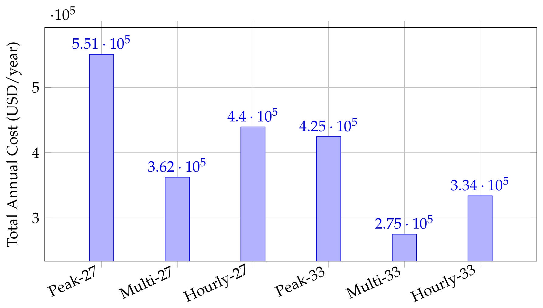
- A comprehensive evaluation of conductor sizing under peak demand, multilevel, and hourly demand representations, showing that the multilevel and hourly formulations produced reductions in the total annual planning costs of up to approximately 35% with respect to the conventional peak demand formulation while satisfying voltage regulation and conductor loading constraints.
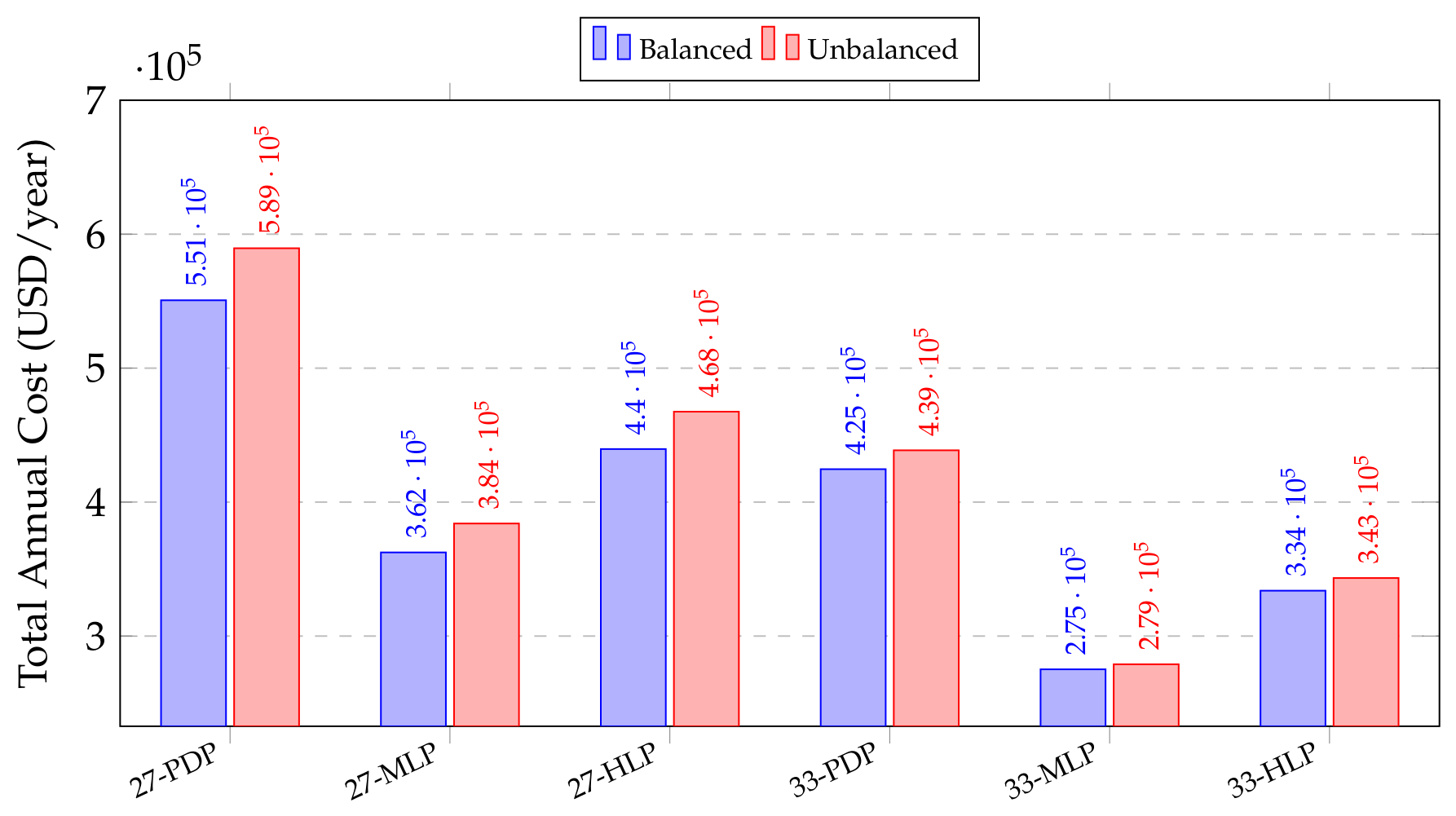
- A quantitative assessment of balanced and unbalanced operating conditions, showing that phase asymmetry modified the optimal conductor sizing, increased the annual operating costs, and mainly affected medium-capacity conductor selections, while the primary feeder reinforcements remained comparatively stable.
- Validation of the proposed native implementation on the 27-, 33-, and IEEE 123-bus benchmark systems, where independent executions exhibited low solution dispersion. For the IEEE 123-bus feeder, the standard deviation remained below 0.7% of the average annual cost under all evaluated demand scenarios, demonstrating low solution dispersion and repeatable optimization results across the evaluated benchmark systems.
- Public release of the developed implementation, benchmark systems, and source code is conducted to facilitate transparency, reproducibility, and future research based on the proposed native DPL framework [31].
1.5. Document Structure
2. Methodology
2.1. Mathematical Formulation of the OCSP
2.2. Operational Constraints
2.3. Load Profile Scenarios
- Peak demand profile (PDP);
- Multilevel load profile (MLP);
- Hourly load profile (HLP).
2.4. Tabu Search-Optimization Framework
| Algorithm 1: Proposed TSA-based OCSP implemented in the DPL |
|
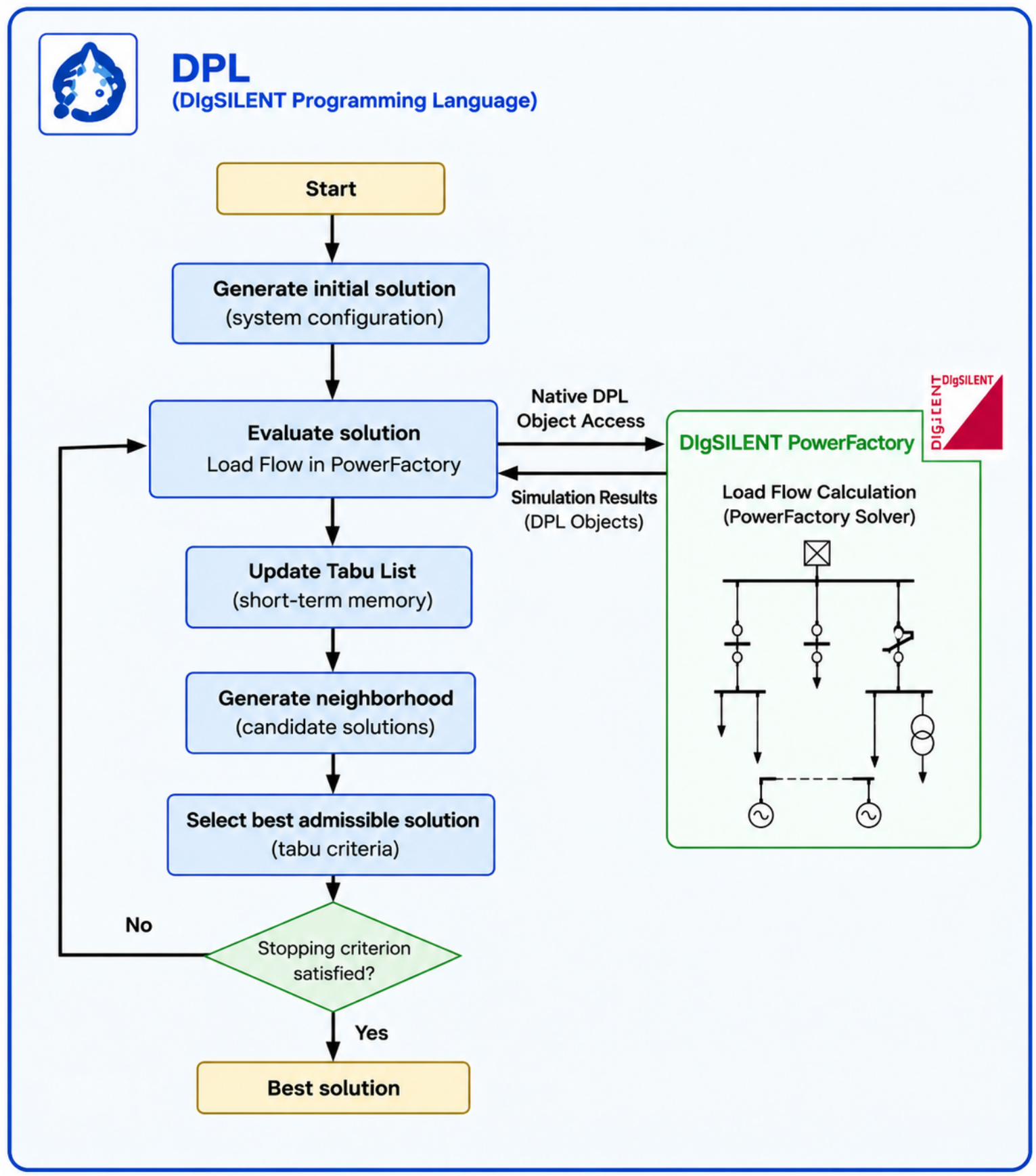
2.5. Native TSA-DPL Implementation and Workflow
3. Test Systems and Simulation Scenarios
3.1. Balanced and Unbalanced Operating Conditions
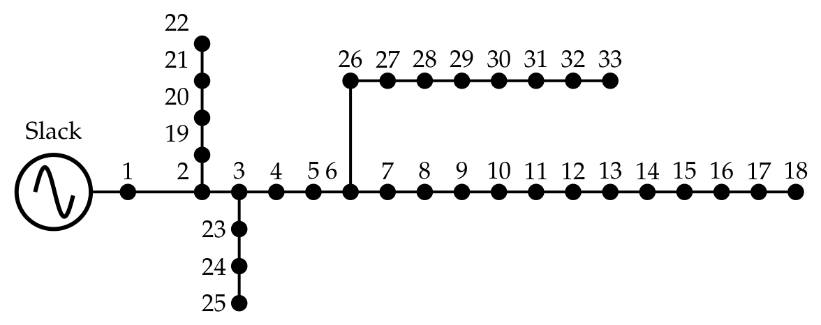
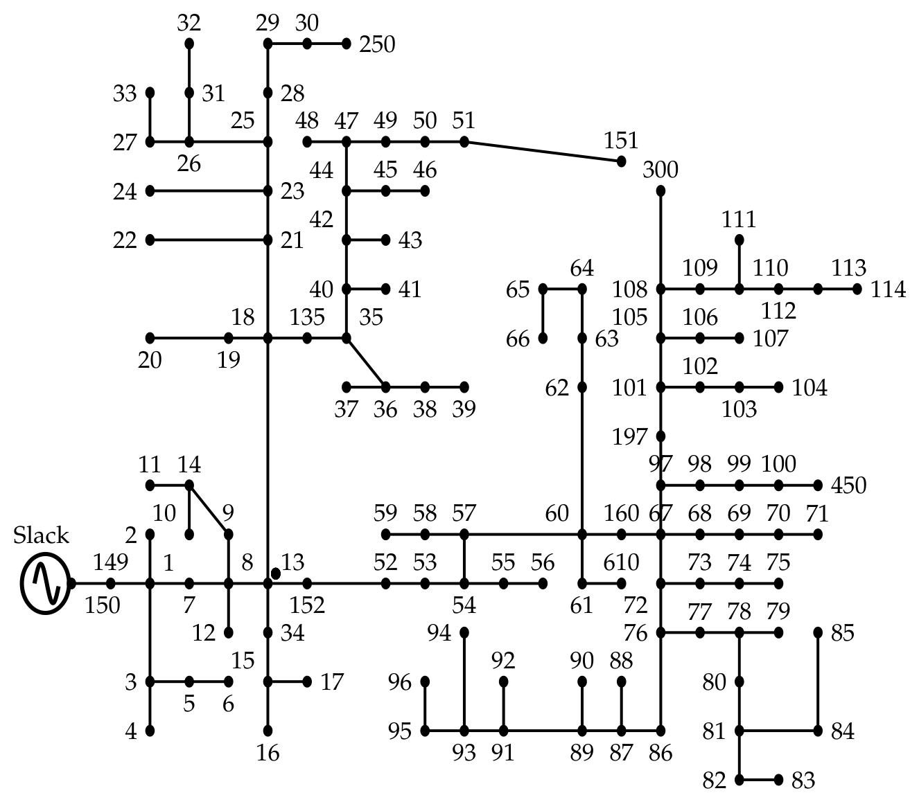
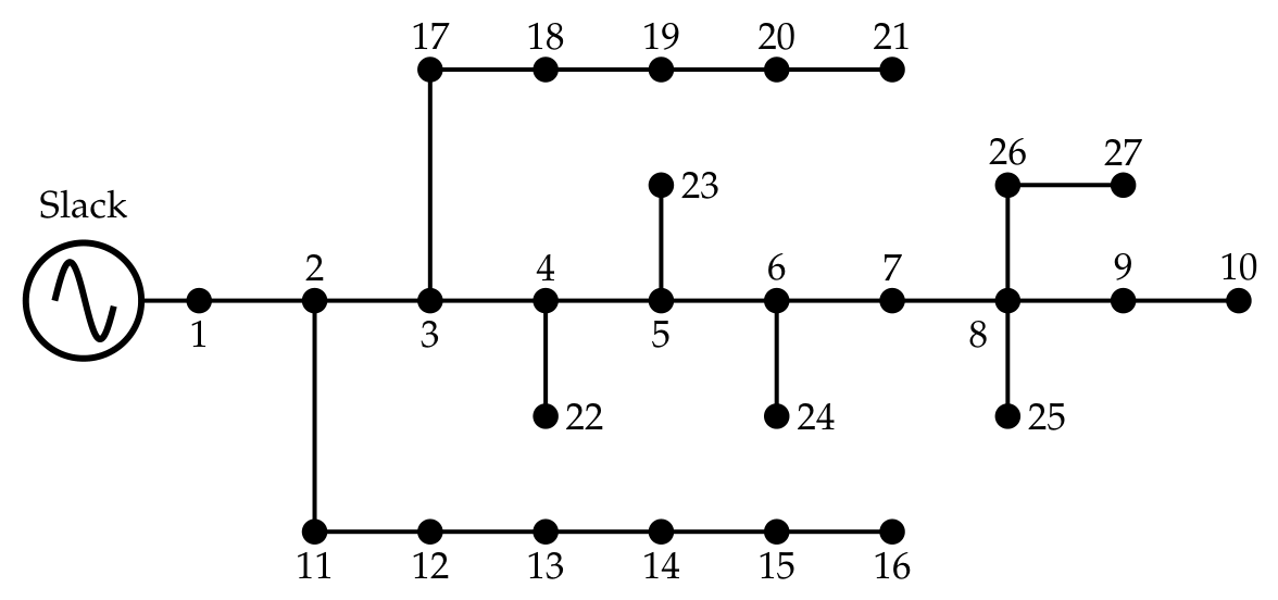
3.2. Evaluated Distribution Systems
3.3. Conductor Catalog and Electrical Parameters
3.4. Model Assumptions
- The distribution systems are operated under radial network configurations.
- The electrical loads are modeled as constant power demands.
- Each line section is assigned a single conductor type selected from the predefined conductor catalog.
- The bus voltage magnitudes are maintained within the allowable limits (0.95–1.05 p.u.).
- Conductor loading is limited to 100% of the rated current-carrying capacity.
- The planning horizon corresponds to one year, and conductor investment costs are included directly in the objective function.
3.5. Simulation Parameters and TSA Configuration
3.6. Performance Metrics
- The total annual cost.
- The operating cost associated with energy losses.
- The conductor investment cost.
- The active power losses.
- The minimum nodal voltage magnitude.
- The maximum branch current loading.
- The computational execution time.
- The TSA’s convergence behavior.
4. Results and Discussion
4.1. Validation Against Literature Benchmarks
4.1.1. Comparison Under Balanced Operating Conditions
4.1.2. Comparison Under Unbalanced Operating Conditions
4.2. Economic Impact of Operating Conditions and Load Profiles
4.2.1. Influence of Load Profiles
4.2.2. Influence of an Unbalanced Operation
4.3. Computational Performance Assessment
4.3.1. Statistical Robustness Analysis
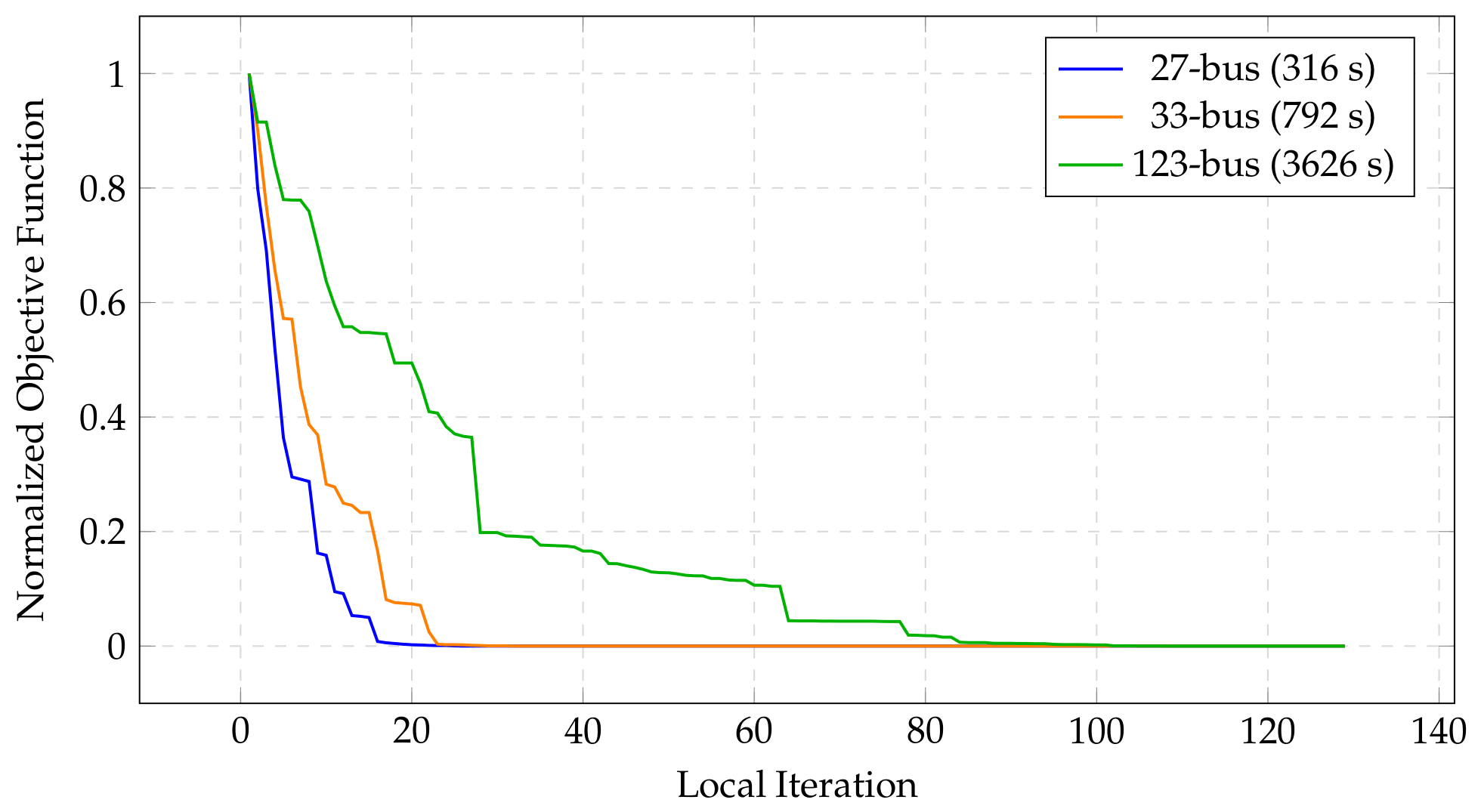
4.3.2. Convergence Behavior
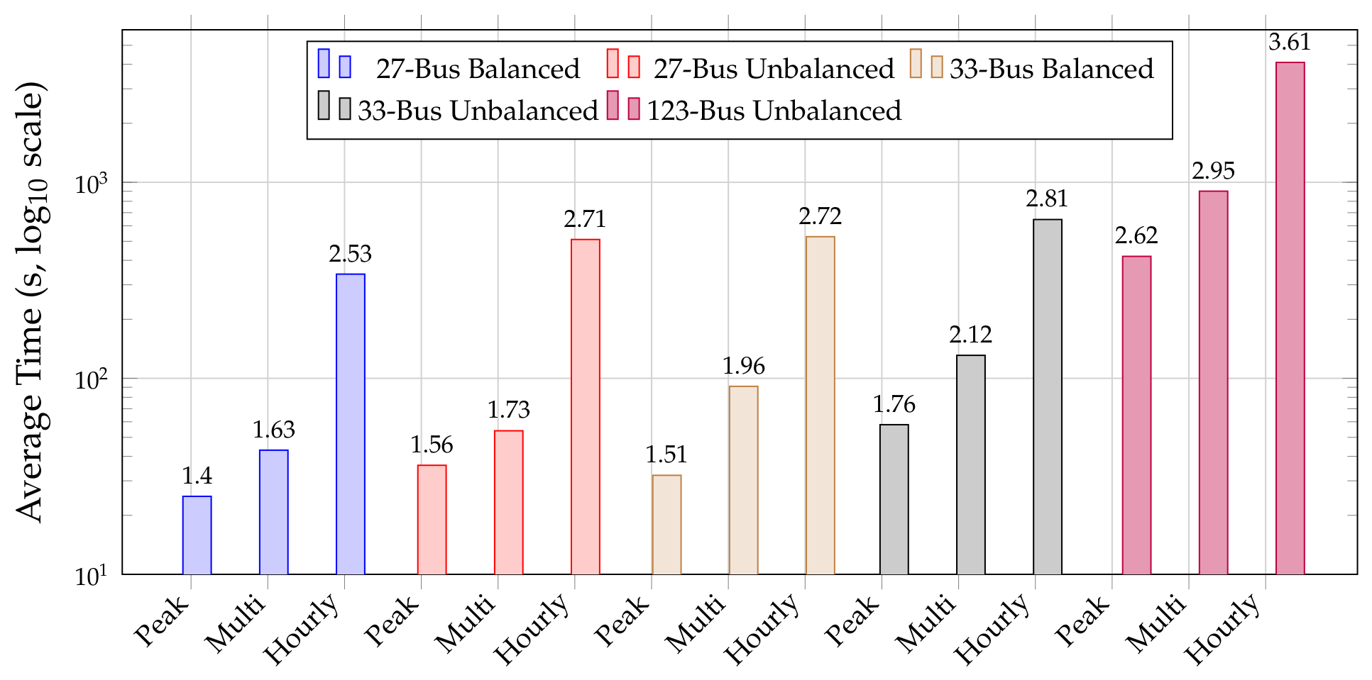
4.3.3. Computation Time Analysis
4.4. Computational Applicability Assessment Using the IEEE 123-Bus System
4.4.1. Optimization Performance Analysis
- (a)
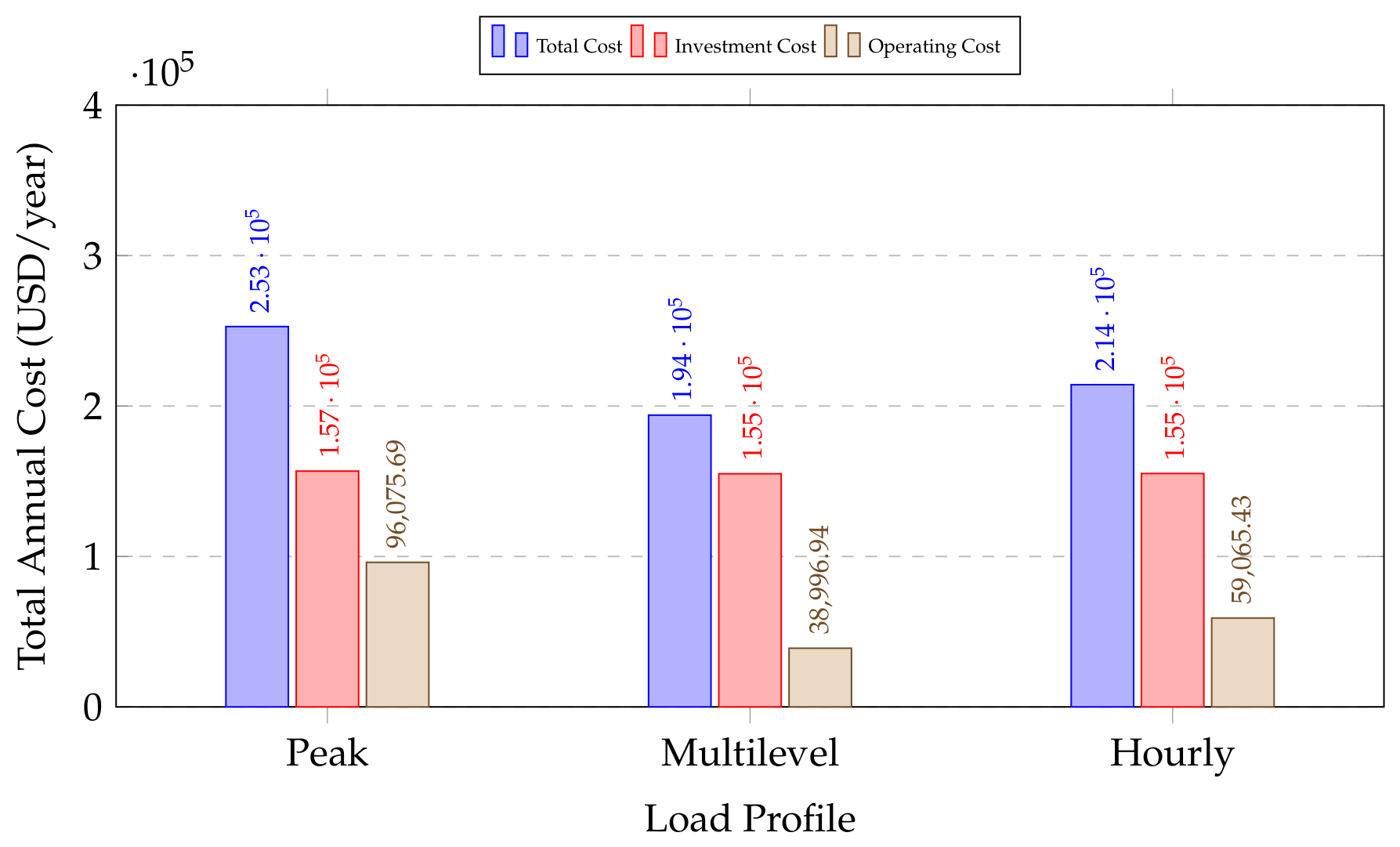
- Comparative cost analysis:
- (b)
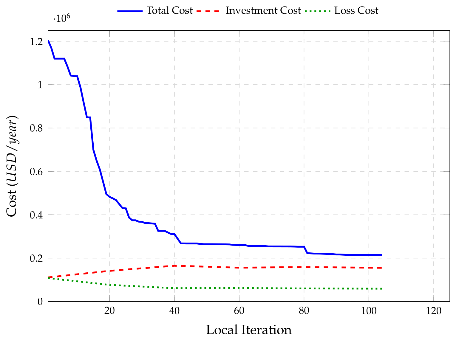
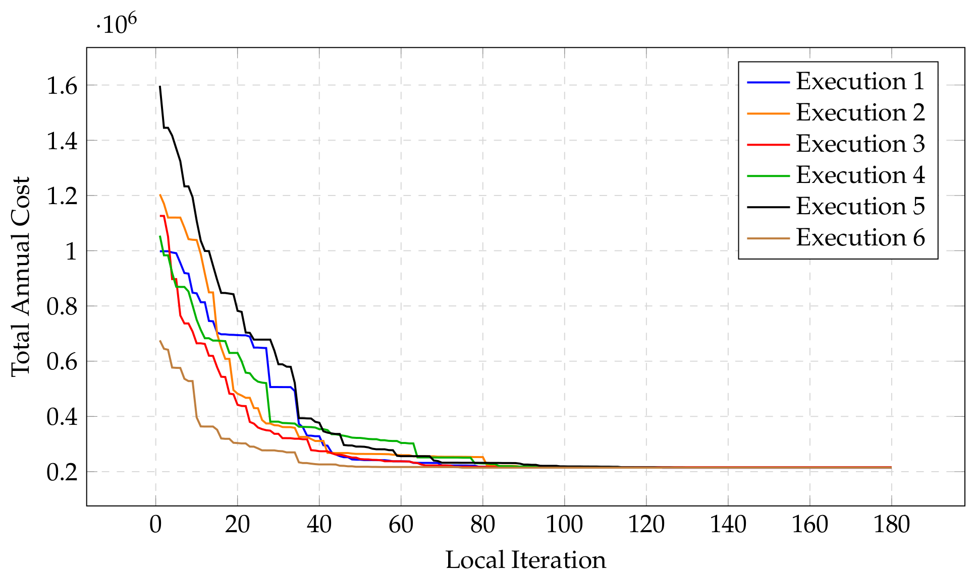
- Cost evolution during local search:
4.4.2. Robustness of the Local Search Process
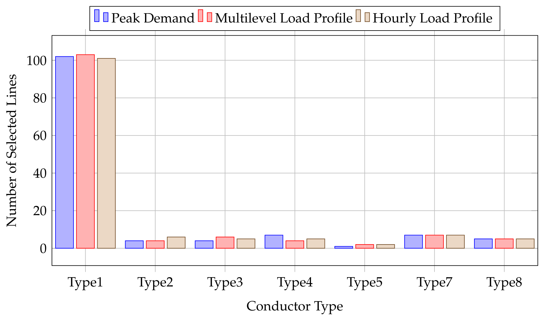
4.4.3. Conductor Allocation Characteristics
4.4.4. Electrical Performance Assessment
- (a)
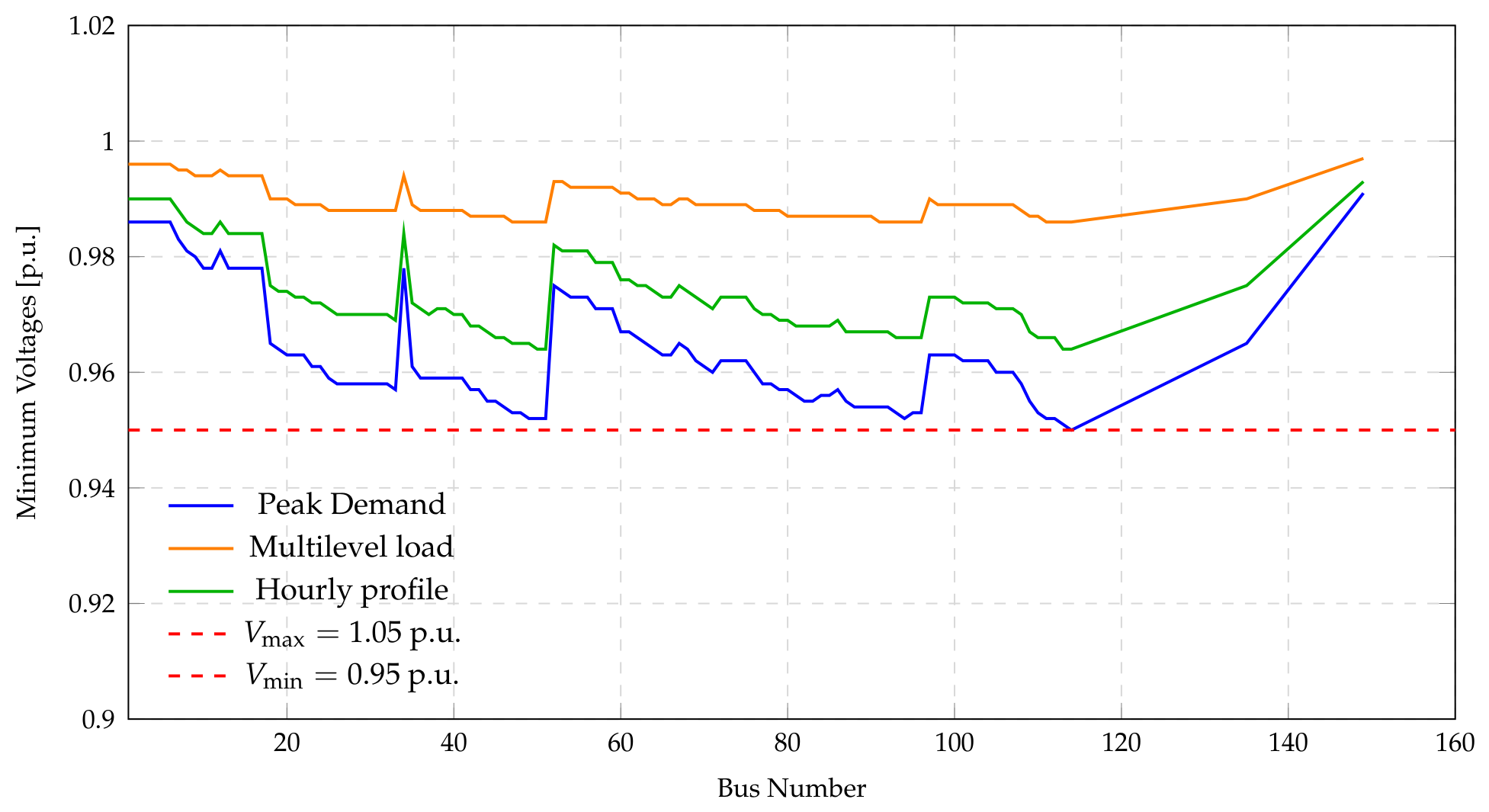
- Voltage performance:
- (b)
- Loss analysis:
- (c)
- Line loading analysis:
4.5. Discussion Regarding the Proposed Native DPL-Based Implementation
5. Conclusions
Author Contributions
Funding
Institutional Review Board Statement
Data Availability Statement
Acknowledgments
Conflicts of Interest
Appendix A
Appendix A.1. Test System Topology and Load Data
Appendix A.1.1. Data 27-Bus System

| Line | Node i | Node j | Lij (km) | (kW) | (kvar) |
|---|---|---|---|---|---|
| 1 | 1 | 2 | 0.55 | 0 | 0 |
| 2 | 2 | 3 | 1.50 | 0 | 0 |
| 3 | 3 | 4 | 0.45 | 297.5 | 184.4 |
| 4 | 4 | 5 | 0.63 | 0 | 0 |
| 5 | 5 | 6 | 0.70 | 255 | 158 |
| 6 | 6 | 7 | 0.55 | 0 | 0 |
| 7 | 7 | 8 | 1.00 | 212.5 | 131.7 |
| 8 | 8 | 9 | 1.25 | 0 | 0 |
| 9 | 9 | 10 | 1.00 | 266.1 | 164.9 |
| 10 | 2 | 11 | 1.00 | 85 | 52.7 |
| 11 | 11 | 12 | 1.23 | 340 | 210.7 |
| 12 | 12 | 13 | 0.75 | 297.5 | 184.4 |
| 13 | 13 | 14 | 0.56 | 191.3 | 118.5 |
| 14 | 14 | 15 | 1.00 | 106.3 | 65.8 |
| 15 | 15 | 16 | 1.00 | 255 | 158 |
| 16 | 3 | 17 | 1.00 | 255 | 158 |
| 17 | 17 | 18 | 0.60 | 127.5 | 79 |
| 18 | 18 | 19 | 0.90 | 297.5 | 184.4 |
| 19 | 19 | 20 | 0.95 | 340 | 210.7 |
| 20 | 20 | 21 | 1.00 | 85 | 52.7 |
| 21 | 4 | 22 | 1.00 | 106.3 | 65.8 |
| 22 | 5 | 23 | 1.00 | 55.3 | 34.2 |
| 23 | 6 | 24 | 0.40 | 69.7 | 43.2 |
| 24 | 8 | 25 | 0.60 | 255 | 158 |
| 25 | 8 | 26 | 0.60 | 63.8 | 39.5 |
| 26 | 26 | 27 | 0.80 | 170 | 105.4 |
| Node j | (kW) | (kvar) | (kW) | (kvar) | (kW) | (kvar) |
|---|---|---|---|---|---|---|
| 2 | 0 | 0 | 0 | 0 | 0 | 0 |
| 3 | 0 | 0 | 0 | 0 | 0 | 0 |
| 4 | 892.5 | 553.2 | 0 | 0 | 0 | 0 |
| 5 | 0 | 0 | 0 | 0 | 0 | 0 |
| 6 | 0 | 0 | 765 | 474 | 0 | 0 |
| 7 | 0 | 0 | 0 | 0 | 0 | 0 |
| 8 | 0 | 0 | 0 | 0 | 637.5 | 395.1 |
| 9 | 0 | 0 | 0 | 0 | 0 | 0 |
| 10 | 0 | 0 | 0 | 0 | 798.3 | 494.7 |
| 11 | 0 | 0 | 255 | 158.1 | 0 | 0 |
| 12 | 1020 | 632.1 | 0 | 0 | 0 | 0 |
| 13 | 446.25 | 276.6 | 446.25 | 276.6 | 0 | 0 |
| 14 | 0 | 0 | 286.95 | 177.75 | 286.95 | 177.75 |
| 15 | 159.45 | 98.7 | 0 | 0 | 159.45 | 98.7 |
| 16 | 0 | 0 | 382.5 | 237 | 382.5 | 237 |
| 17 | 1 | 0 | 765 | 474 | 0 | 0 |
| 18 | 382.5 | 237 | 0 | 0 | 0 | 0 |
| 19 | 446.25 | 276.6 | 446.25 | 276.6 | 0 | 0 |
| 20 | 0 | 0 | 510 | 316.05 | 510 | 316.05 |
| 21 | 127.5 | 79.05 | 0 | 0 | 127.5 | 79.05 |
| 22 | 0 | 0 | 159.75 | 98.7 | 159.75 | 98.7 |
| 23 | 165.9 | 102.6 | 0 | 0 | 0 | 0 |
| 24 | 0 | 0 | 0 | 0 | 209.1 | 129.6 |
| 25 | 255 | 158 | 255 | 158 | 255 | 158 |
| 26 | 63.8 | 39.5 | 63.8 | 39.5 | 63.8 | 39.5 |
| 27 | 170 | 105.4 | 170 | 105.4 | 170 | 105.4 |
Appendix A.1.2. The 33-Bus System
| Line | Node i | Node j | (km) | (kW) | (kvar) |
|---|---|---|---|---|---|
| 1 | 1 | 2 | 0.0699 | 100 | 60 |
| 2 | 2 | 3 | 0.3720 | 90 | 40 |
| 3 | 3 | 4 | 0.2762 | 120 | 80 |
| 4 | 4 | 5 | 0.2876 | 60 | 30 |
| 5 | 5 | 6 | 0.7630 | 60 | 20 |
| 6 | 6 | 7 | 0.4030 | 200 | 100 |
| 7 | 7 | 8 | 1.4733 | 200 | 100 |
| 8 | 8 | 9 | 0.8850 | 60 | 20 |
| 9 | 9 | 10 | 0.8900 | 60 | 20 |
| 10 | 10 | 11 | 0.1308 | 45 | 30 |
| 11 | 11 | 12 | 0.2491 | 60 | 35 |
| 12 | 12 | 13 | 1.3115 | 60 | 35 |
| 13 | 13 | 14 | 0.6272 | 120 | 80 |
| 14 | 14 | 15 | 0.5585 | 60 | 10 |
| 15 | 15 | 16 | 0.6457 | 60 | 20 |
| 16 | 16 | 17 | 1.5050 | 60 | 20 |
| 17 | 17 | 18 | 0.6530 | 90 | 40 |
| 18 | 2 | 19 | 0.1603 | 90 | 40 |
| 19 | 19 | 20 | 1.4298 | 90 | 40 |
| 20 | 20 | 21 | 0.4439 | 90 | 40 |
| 21 | 21 | 22 | 0.8231 | 90 | 40 |
| 22 | 3 | 23 | 0.3798 | 90 | 40 |
| 23 | 23 | 24 | 0.8035 | 420 | 200 |
| 24 | 24 | 25 | 0.7985 | 420 | 200 |
| 25 | 6 | 26 | 0.1532 | 60 | 25 |
| 26 | 26 | 27 | 0.2145 | 60 | 25 |
| 27 | 27 | 28 | 0.9963 | 60 | 20 |
| 28 | 28 | 29 | 0.7524 | 120 | 70 |
| 29 | 29 | 30 | 0.3830 | 200 | 600 |
| 30 | 30 | 31 | 0.9687 | 150 | 70 |
| 31 | 31 | 32 | 0.3362 | 210 | 100 |
| 32 | 32 | 33 | 0.4356 | 60 | 40 |
| Node j | (kW) | (kvar) | (kW) | (kvar) | (kW) | (kvar) |
|---|---|---|---|---|---|---|
| 2 | 100 | 50 | 100 | 60 | 0 | 0 |
| 3 | 90 | 0 | 90 | 40 | 0 | 0 |
| 4 | 120 | 75 | 120 | 80 | 150 | 90 |
| 5 | 60 | 20 | 60 | 30 | 60 | 30 |
| 6 | 60 | 18 | 60 | 20 | 60 | 20 |
| 7 | 200 | 150 | 0 | 0 | 100 | 100 |
| 8 | 200 | 0 | 200 | 100 | 0 | 0 |
| 9 | 60 | 60 | 0 | 0 | 0 | 0 |
| 10 | 60 | 60 | 60 | 20 | 0 | 0 |
| 11 | 45 | 30 | 45 | 30 | 45 | 30 |
| 12 | 0 | 0 | 60 | 35 | 155 | 100 |
| 13 | 60 | 110 | 60 | 35 | 60 | 35 |
| 14 | 120 | 80 | 190 | 80 | 120 | 80 |
| 15 | 60 | 10 | 60 | 50 | 60 | 10 |
| 16 | 60 | 20 | 110 | 80 | 60 | 20 |
| 17 | 60 | 20 | 150 | 95 | 0 | 0 |
| 18 | 90 | 40 | 100 | 0 | 90 | 40 |
| 19 | 0 | 0 | 0 | 0 | 90 | 40 |
| 20 | 210 | 50 | 85 | 40 | 70 | 75 |
| 21 | 90 | 40 | 110 | 40 | 110 | 20 |
| 22 | 300 | 400 | 0 | 0 | 90 | 40 |
| 23 | 90 | 50 | 70 | 0 | 0 | 0 |
| 24 | 420 | 200 | 420 | 200 | 420 | 200 |
| 25 | 120 | 75 | 0 | 0 | 150 | 100 |
| 26 | 60 | 25 | 80 | 25 | 0 | 0 |
| 27 | 0 | 0 | 80 | 25 | 0 | 0 |
| 28 | 60 | 20 | 48 | 24 | 60 | 20 |
| 29 | 120 | 70 | 185 | 75 | 120 | 70 |
| 30 | 200 | 600 | 400 | 400 | 500 | 600 |
| 31 | 150 | 70 | 120 | 90 | 150 | 70 |
| 32 | 210 | 100 | 120 | 35 | 210 | 100 |
| 33 | 60 | 40 | 100 | 750 | 0 | 0 |
Appendix A.1.3. IEEE 123-Bus System
| Line | Node i | Node j | (ft) | (kW) | (kvar) | (kW) | (kvar) | (kW) | (kvar) |
|---|---|---|---|---|---|---|---|---|---|
| 1 | 1 | 2 | 175 | 0 | 0 | 0 | 20 | 10 | 0 |
| 2 | 1 | 3 | 250 | 0 | 0 | 0 | 0 | 0 | 0 |
| 3 | 1 | 7 | 300 | 20 | 10 | 20 | 0 | 0 | 0 |
| 4 | 3 | 4 | 200 | 0 | 0 | 0 | 0 | 0 | 40 |
| 5 | 3 | 5 | 325 | 0 | 0 | 0 | 0 | 0 | 20 |
| 6 | 5 | 6 | 250 | 0 | 0 | 0 | 0 | 0 | 40 |
| 7 | 7 | 8 | 200 | 0 | 0 | 0 | 0 | 0 | 0 |
| 8 | 8 | 12 | 225 | 0 | 0 | 0 | 20 | 10 | 0 |
| 9 | 8 | 9 | 225 | 40 | 20 | 40 | 0 | 0 | 0 |
| 10 | 8 | 13 | 300 | 0 | 0 | 0 | 0 | 0 | 0 |
| 11 | 9 | 14 | 425 | 0 | 0 | 0 | 0 | 0 | 0 |
| 12 | 13 | 34 | 150 | 0 | 0 | 0 | 0 | 0 | 40 |
| 13 | 13 | 18 | 825 | 0 | 0 | 0 | 0 | 0 | 0 |
| 14 | 14 | 11 | 250 | 40 | 20 | 40 | 0 | 0 | 0 |
| 15 | 14 | 10 | 250 | 20 | 10 | 20 | 0 | 0 | 0 |
| 16 | 15 | 16 | 375 | 0 | 0 | 0 | 0 | 0 | 40 |
| 17 | 15 | 17 | 350 | 0 | 0 | 0 | 0 | 0 | 20 |
| 18 | 18 | 19 | 250 | 40 | 20 | 40 | 0 | 0 | 0 |
| 19 | 18 | 21 | 300 | 0 | 0 | 0 | 0 | 0 | 0 |
| 20 | 19 | 20 | 325 | 40 | 20 | 40 | 0 | 0 | 0 |
| 21 | 21 | 22 | 525 | 0 | 0 | 0 | 40 | 20 | 0 |
| 22 | 21 | 23 | 250 | 0 | 0 | 0 | 0 | 0 | 0 |
| 23 | 23 | 24 | 550 | 0 | 0 | 0 | 0 | 0 | 40 |
| 24 | 23 | 25 | 275 | 0 | 0 | 0 | 0 | 0 | 0 |
| 25 | 25 | 26 | 350 | 0 | 0 | 0 | 0 | 0 | 0 |
| 26 | 25 | 28 | 200 | 40 | 20 | 40 | 0 | 0 | 0 |
| 27 | 26 | 27 | 275 | 0 | 0 | 0 | 0 | 0 | 0 |
| 28 | 26 | 31 | 225 | 0 | 0 | 0 | 0 | 0 | 20 |
| 29 | 27 | 33 | 500 | 40 | 20 | 40 | 0 | 0 | 0 |
| 30 | 28 | 29 | 300 | 40 | 20 | 40 | 0 | 0 | 0 |
| 31 | 29 | 30 | 350 | 0 | 0 | 0 | 0 | 0 | 40 |
| 32 | 30 | 250 | 200 | 0 | 0 | 0 | 0 | 0 | 0 |
| 33 | 31 | 32 | 300 | 0 | 0 | 0 | 0 | 0 | 20 |
| 34 | 34 | 15 | 100 | 0 | 0 | 0 | 0 | 0 | 0 |
| 35 | 35 | 36 | 650 | 0 | 0 | 0 | 0 | 0 | 0 |
| 36 | 35 | 40 | 250 | 0 | 0 | 0 | 0 | 0 | 0 |
| 37 | 36 | 37 | 300 | 40 | 20 | 40 | 0 | 0 | 0 |
| 38 | 36 | 38 | 250 | 0 | 0 | 0 | 20 | 10 | 0 |
| 39 | 38 | 39 | 325 | 0 | 0 | 0 | 20 | 10 | 0 |
| 40 | 40 | 41 | 325 | 0 | 0 | 0 | 0 | 0 | 20 |
| 41 | 40 | 42 | 250 | 20 | 10 | 20 | 0 | 0 | 0 |
| 42 | 42 | 43 | 500 | 0 | 0 | 0 | 40 | 20 | 0 |
| 43 | 42 | 44 | 200 | 0 | 0 | 0 | 0 | 0 | 0 |
| 44 | 44 | 45 | 200 | 20 | 10 | 20 | 0 | 0 | 0 |
| 45 | 44 | 47 | 250 | 35 | 25 | 35 | 35 | 25 | 35 |
| 46 | 45 | 46 | 300 | 20 | 10 | 20 | 0 | 0 | 0 |
| 47 | 47 | 48 | 150 | 70 | 50 | 70 | 70 | 50 | 70 |
| 48 | 47 | 49 | 250 | 35 | 25 | 35 | 70 | 50 | 35 |
| 49 | 49 | 50 | 250 | 0 | 0 | 0 | 0 | 0 | 40 |
| 50 | 50 | 51 | 250 | 20 | 10 | 20 | 0 | 0 | 0 |
| 51 | 51 | 151 | 500 | 0 | 0 | 0 | 0 | 0 | 0 |
| 52 | 52 | 53 | 200 | 40 | 20 | 40 | 0 | 0 | 0 |
| 53 | 53 | 54 | 125 | 0 | 0 | 0 | 0 | 0 | 0 |
| 54 | 54 | 55 | 275 | 20 | 10 | 20 | 0 | 0 | 0 |
| 55 | 54 | 57 | 350 | 0 | 0 | 0 | 0 | 0 | 0 |
| 56 | 55 | 56 | 275 | 0 | 0 | 0 | 20 | 10 | 0 |
| 57 | 57 | 58 | 250 | 0 | 0 | 0 | 20 | 10 | 0 |
| 58 | 57 | 60 | 750 | 20 | 10 | 20 | 0 | 0 | 0 |
| 59 | 58 | 59 | 250 | 0 | 0 | 0 | 20 | 10 | 0 |
| Line | Node i | Node j | (ft) | (kW) | (kvar) | (kW) | (kvar) | (kW) | (kvar) |
|---|---|---|---|---|---|---|---|---|---|
| 60 | 60 | 61 | 550 | 0 | 0 | 0 | 0 | 0 | 0 |
| 61 | 60 | 62 | 250 | 0 | 0 | 0 | 0 | 0 | 40 |
| 62 | 62 | 63 | 175 | 40 | 20 | 40 | 0 | 0 | 0 |
| 63 | 63 | 64 | 350 | 0 | 0 | 0 | 75 | 35 | 0 |
| 64 | 64 | 65 | 425 | 35 | 25 | 35 | 35 | 25 | 70 |
| 65 | 65 | 66 | 325 | 0 | 0 | 0 | 0 | 0 | 75 |
| 66 | 67 | 68 | 200 | 20 | 10 | 20 | 0 | 0 | 0 |
| 67 | 67 | 72 | 275 | 0 | 0 | 0 | 0 | 0 | 0 |
| 68 | 67 | 97 | 250 | 0 | 0 | 0 | 0 | 0 | 0 |
| 69 | 68 | 69 | 275 | 40 | 20 | 40 | 0 | 0 | 0 |
| 70 | 69 | 70 | 325 | 20 | 10 | 20 | 0 | 0 | 0 |
| 71 | 70 | 71 | 275 | 40 | 20 | 40 | 0 | 0 | 0 |
| 72 | 72 | 73 | 275 | 0 | 0 | 0 | 0 | 0 | 40 |
| 73 | 72 | 76 | 200 | 105 | 80 | 105 | 70 | 50 | 70 |
| 74 | 73 | 74 | 350 | 0 | 0 | 0 | 0 | 0 | 40 |
| 75 | 74 | 75 | 400 | 0 | 0 | 0 | 0 | 0 | 40 |
| 76 | 76 | 77 | 400 | 0 | 0 | 0 | 40 | 20 | 0 |
| 77 | 76 | 86 | 700 | 0 | 0 | 0 | 20 | 10 | 0 |
| 78 | 77 | 78 | 100 | 0 | 0 | 0 | 0 | 0 | 0 |
| 79 | 78 | 79 | 225 | 40 | 20 | 40 | 0 | 0 | 0 |
| 80 | 78 | 80 | 475 | 0 | 0 | 0 | 40 | 20 | 0 |
| 81 | 80 | 81 | 475 | 0 | 0 | 0 | 0 | 0 | 0 |
| 82 | 81 | 82 | 250 | 40 | 20 | 40 | 0 | 0 | 0 |
| 83 | 81 | 84 | 675 | 0 | 0 | 0 | 0 | 0 | 20 |
| 84 | 82 | 83 | 250 | 0 | 0 | 0 | 0 | 0 | 20 |
| 85 | 84 | 85 | 475 | 0 | 0 | 0 | 0 | 0 | 40 |
| 86 | 86 | 87 | 450 | 0 | 0 | 0 | 40 | 20 | 0 |
| 87 | 87 | 88 | 175 | 40 | 20 | 40 | 0 | 0 | 0 |
| 88 | 87 | 89 | 275 | 0 | 0 | 0 | 0 | 0 | 0 |
| 89 | 89 | 90 | 225 | 0 | 0 | 0 | 40 | 20 | 0 |
| 90 | 89 | 91 | 225 | 0 | 0 | 0 | 0 | 0 | 0 |
| 91 | 91 | 92 | 300 | 0 | 0 | 0 | 0 | 0 | 40 |
| 92 | 91 | 93 | 225 | 0 | 0 | 0 | 0 | 0 | 0 |
| 93 | 93 | 94 | 275 | 40 | 20 | 40 | 0 | 0 | 0 |
| 94 | 93 | 95 | 300 | 0 | 0 | 0 | 20 | 10 | 0 |
| 95 | 95 | 96 | 200 | 0 | 0 | 0 | 20 | 10 | 0 |
| 96 | 97 | 98 | 275 | 40 | 20 | 40 | 0 | 0 | 0 |
| 97 | 98 | 99 | 550 | 0 | 0 | 0 | 40 | 20 | 0 |
| 98 | 99 | 100 | 300 | 0 | 0 | 0 | 0 | 0 | 40 |
| 99 | 100 | 450 | 800 | 0 | 0 | 0 | 0 | 0 | 0 |
| 100 | 101 | 102 | 225 | 0 | 0 | 0 | 0 | 0 | 20 |
| 101 | 101 | 105 | 275 | 0 | 0 | 0 | 0 | 0 | 0 |
| 102 | 102 | 103 | 325 | 0 | 0 | 0 | 0 | 0 | 40 |
| 103 | 103 | 104 | 700 | 0 | 0 | 0 | 0 | 0 | 40 |
| 104 | 105 | 106 | 225 | 0 | 0 | 0 | 40 | 20 | 0 |
| 105 | 105 | 108 | 325 | 0 | 0 | 0 | 0 | 0 | 0 |
| 106 | 106 | 107 | 575 | 0 | 0 | 0 | 40 | 20 | 0 |
| 107 | 108 | 109 | 450 | 40 | 20 | 40 | 0 | 0 | 0 |
| 108 | 108 | 300 | 1000 | 0 | 0 | 0 | 0 | 0 | 0 |
| 109 | 109 | 110 | 300 | 0 | 0 | 0 | 0 | 0 | 0 |
| 110 | 110 | 111 | 575 | 20 | 10 | 20 | 0 | 0 | 0 |
| 111 | 110 | 112 | 125 | 20 | 10 | 20 | 0 | 0 | 0 |
| 112 | 112 | 113 | 525 | 40 | 20 | 40 | 0 | 0 | 0 |
| 113 | 113 | 114 | 325 | 20 | 10 | 20 | 0 | 0 | 0 |
| 114 | 135 | 35 | 375 | 40 | 20 | 40 | 0 | 0 | 0 |
| 115 | 149 | 1 | 400 | 40 | 20 | 40 | 0 | 0 | 0 |
| 116 | 152 | 52 | 400 | 40 | 20 | 40 | 0 | 0 | 0 |
| Line | Node i | Node j | (ft) | (kW) | (kvar) | (kW) | (kvar) | (kW) | (kvar) |
|---|---|---|---|---|---|---|---|---|---|
| 117 | 160 | 67 | 350 | 0 | 0 | 0 | 0 | 0 | 0 |
| 118 | 197 | 101 | 250 | 0 | 0 | 0 | 0 | 0 | 0 |
| 119 | 13 | 152 | 2 | 0 | 0 | 0 | 0 | 0 | 0 |
| 120 | 18 | 135 | 2 | 0 | 0 | 0 | 0 | 0 | 0 |
| 121 | 60 | 160 | 2 | 0 | 0 | 0 | 0 | 0 | 0 |
| 122 | 61 | 610 | 1 | 0 | 0 | 0 | 0 | 0 | 0 |
| 123 | 97 | 197 | 2 | 0 | 0 | 0 | 0 | 0 | 0 |
| 124 | 150 | 149 | 2 | 0 | 0 | 0 | 0 | 0 | 0 |
Appendix A.2. Conductor Selection Results
Appendix A.2.1. Conductor Selection for the 27-Bus System
| Case | Method | Gauges | Annual Cost (USD) |
|---|---|---|---|
| Peak | TSA | 550,668.371 | |
| Hourly | TSA | 439,566.045 | |
| Multilevel | TSA | 362,431.588 |
| Case | Method | Gauges | Annual Cost (USD) |
|---|---|---|---|
| Peak | TSA | 589,482.447 | |
| Hourly | TSA | 467,507.064 | |
| Multilevel | TSA | 383,998.001 |
Appendix A.2.2. Conductor Selection for the 33-Bus System
| Case | Method | Gauges | Annual Cost (USD) |
|---|---|---|---|
| Peak | TSA | 424,561.302 | |
| Hourly | TSA | 333,865.488 | |
| Multilevel | TSA | 275,154.716 |
| Case | Method | Gauges | Annual Cost (USD) |
|---|---|---|---|
| Peak | TSA | 438,637.176 | |
| Hourly | TSA | 343,332.933 | |
| Multilevel | TSA | 278,939.389 |
Appendix A.2.3. Conductor Selection for the 123-Bus System
| Case | Method | Gauges | Annual Cost (USD) |
|---|---|---|---|
| Peak | TSA | 252,799.946 | |
| Multilevel | TSA | 193,948.013 | |
| Hourly | TSA | 214,194.516 |
References
- Adham, M.; Keene, S.; Bass, R.B. Distributed Energy Resources: A Systematic Literature Review. Energy Rep. 2025, 13, 1980–1999. [Google Scholar] [CrossRef] [Scilit]
- Marlés-Sáenz, E.; Gómez-Luna, E.; Guerrero, J.M.; Vasquez, J.C. Analysis of Impacts in Electric Power Grids Due to the Integration of Distributed Energy Resources. Energies 2025, 18, 745. [Google Scholar] [CrossRef] [Scilit]
- Waswa, L.; Chihota, M.J.; Bekker, B. Toward Optimal Active Distribution Network Planning: A Critical Review of Conductor Size Selection Methods. IEEE Access 2023, 11, 144812–144830. [Google Scholar] [CrossRef] [Scilit]
- Pham, N.V.; Pham, C.C. A MISOCP-based methodology for optimally selecting conductor cross-sections in electricity distribution grids considering daily patterns and voltage-dependence of loads. Eng. Res. Express 2026, 8, 065320. [Google Scholar] [CrossRef] [Scilit]
- Franco, J.F.; Rider, M.J.; Lavorato, M.; Romero, R. Optimal Conductor Size Selection and Reconductoring in Radial Distribution Systems Using a Mixed-Integer LP Approach. IEEE Trans. Power Syst. 2013, 28, 10–20. [Google Scholar] [CrossRef] [Scilit]
- Zdraveski, V.; Todorovski, M. Conductor size selection in radial distribution networks using robust optimization. Sustain. Energy Grids Netw. 2025, 43, 101730. [Google Scholar] [CrossRef] [Scilit]
- Ponce, D.; Aguila Téllez, A.; Krishnan, N. Optimal Selection of Conductors in Distribution System Designs Using Multi-Criteria Decision. Energies 2023, 16, 7167. [Google Scholar] [CrossRef] [Scilit]
- Mandal, S.; Pahwa, A. Optimal selection of conductors for distribution feeders. IEEE Trans. Power Syst. 2002, 17, 192–197. [Google Scholar] [CrossRef]
- Joshi, D.; Burada, S.; Mistry, K.D. Distribution system planning with optimal conductor selection. In Proceedings of the 2017 Recent Developments in Control, Automation & Power Engineering (RDCAPE), Noida, India, 26–27 October 2017; IEEE: Piscataway, NJ, USA, 2017; pp. 263–268. [Google Scholar] [CrossRef] [Scilit]
- Vega-Forero, J.A.; Ramos-Castellanos, J.S.; Montoya, O.D. Application of the Generalized Normal Distribution Optimization Algorithm to the Optimal Selection of Conductors in Three-Phase Asymmetric Distribution Networks. Energies 2023, 16, 1311. [Google Scholar] [CrossRef] [Scilit]
- Pradilla-Rozo, J.D.; Vega-Forero, J.A.; Montoya, O.D. Application of the Gradient-Based Metaheuristic Optimizerto Solve the Optimal Conductor Selection Problemin Three-Phase Asymmetric Distribution Networks. Energies 2023, 16, 888. [Google Scholar] [CrossRef] [Scilit]
- Nivia Torres, D.J.; Salazar Alarcón, G.A.; Montoya Giraldo, O.D. Selección óptima de conductores en redes de distribución trifásicas utilizando el algoritmo metaheurístico de Newton. Ingeniería 2022, 27, e19303. [Google Scholar] [CrossRef] [Scilit]
- Martínez-Gil, J.F.; Moyano-García, N.A.; Montoya, O.D.; Alarcon-Villamil, J.A. Optimal Selection of Conductors in Three-Phase Distribution Networks Using a Discrete Version of the Vortex Search Algorithm. Computation 2021, 9, 80. [Google Scholar] [CrossRef] [Scilit]
- Pfitscher, L.; Bernardon, D.; Canha, L.; Montagner, V.; Abaide, A.; Saldanha, J. A methodology for real time analysis of parallelism of distribution networks. Electr. Power Syst. Res. 2013, 105, 1–8. [Google Scholar] [CrossRef] [Scilit]
- Gonzalez-Longatt, F.; Alhejaj, S.; Marano-Marcolini, A.; Rueda Torres, J.L. Probabilistic Load-Flow Using Analysis Using DPL Scripting Language. In Advanced Smart Grid Functionalities Based on PowerFactory; Springer International Publishing: Cham, Switzerland, 2017; pp. 93–124. [Google Scholar] [CrossRef] [Scilit]
- Zare, M.; Azizipanah-Abarghooee, R.; Malekpour, M.; Terzija, V. Optimal PMU Placement Framework Under Observability Redundancy and Contingency—An Evolutionary Algorithm Using DIgSILENT Programming Language Module. In Advanced Smart Grid Functionalities Based on PowerFactory; Springer International Publishing: Cham, Switzerland, 2017; pp. 241–277. [Google Scholar] [CrossRef] [Scilit]
- Cepeda, J.C.; Rueda, J.L.; Erlich, I.; Korai, A.W.; Gonzalez-Longatt, F.M. Mean–Variance Mapping Optimization Algorithm for Power System Applications in DIgSILENT PowerFactory. In PowerFactory Applications for Power System Analysis; Springer International Publishing: Cham, Switzerland, 2014; pp. 267–295. [Google Scholar] [CrossRef] [Scilit]
- Singh, S.P.; Kanwar, N.; Saraswat, A. A Multi-Period Load Flow Framework for Active Distribution Network Using DIgSILENT PowerFactory Software. In Flexible Electronics for Electric Vehicles; Springer: Singapore, 2022; pp. 367–375. [Google Scholar] [CrossRef] [Scilit]
- Rao, R.S.; Satish, K.; Narasimham, S.V.L. Optimal Conductor Size Selection in Distribution Systems Using the Harmony Search Algorithm with a Differential Operator. Electr. Power Compon. Syst. 2011, 40, 41–56. [Google Scholar] [CrossRef] [Scilit]
- Manikandan, S.; Sasitharan, S.; Rao, J.V.; Moorthy, V. Analysis of optimal conductor selection for radial distribution systems using DPSO. In Proceedings of the 2016 3rd International Conference on Electrical Energy Systems (ICEES), Chennai, India, 17–19 March 2016; IEEE: Piscataway, NJ, USA, 2016; pp. 96–101. [Google Scholar] [CrossRef] [Scilit]
- Pereira Junior, B.R.; Cossi, A.M.; Contreras, J.; Mantovani, J.R.S. Multiobjective multistage distribution system planning using tabu search. IET Gener. Transm. Distrib. 2014, 8, 35–45. [Google Scholar] [CrossRef] [Scilit]
- Ziegler, D.U.; Prettico, G.; Mateo, C.; Gómez San Román, T. Methodology for integrating flexibility into realistic large-scale distribution network planning using Tabu search. Int. J. Electr. Power Energy Syst. 2023, 152, 109201. [Google Scholar] [CrossRef] [Scilit]
- Gallego Pareja, L.A.; López-Lezama, J.M.; Gómez Carmona, O. A MILP Model for Optimal Conductor Selection and Capacitor Banks Placement in Primary Distribution Systems. Energies 2023, 16, 4340. [Google Scholar] [CrossRef] [Scilit]
- Falaghi, H.; Ramezani, M.; Haghifam, M.R.; Milani, K. Optimal selection of conductors in radial distribution systems with time varying load. In Proceedings of the 18th International Conference and Exhibition on Electricity Distribution (CIRED 2005), Turin, Italy, 6–9 June 2005; IEEE: Piscataway, NJ, USA, 2005; pp. 1–4. [Google Scholar] [CrossRef] [Scilit]
- Garces, A. A Linear Three-Phase Load Flow for Power Distribution Systems. IEEE Trans. Power Syst. 2016, 31, 827–828. [Google Scholar] [CrossRef] [Scilit]
- Shen, T.; Li, Y.; Xiang, J. A Graph-Based Power Flow Method for Balanced Distribution Systems. Energies 2018, 11, 511. [Google Scholar] [CrossRef] [Scilit]
- Zhang, X.; Hua, W.; Liu, Y.; Duan, J.; Tang, Z.; Liu, J. Reinforcement learning for active distribution network planning based on Monte Carlo tree search. Int. J. Electr. Power Energy Syst. 2022, 138, 107885. [Google Scholar] [CrossRef] [Scilit]
- Glover, D.; Krishnamoorthy, G.; Ren, H.; Dubey, A.; Gebremedhin, A. Deep Reinforcement Learning for Distribution System Operations: A Tutorial and Survey. Proc. IEEE 2025, 113, 557–585. [Google Scholar] [CrossRef] [Scilit]
- Shuaijia, H.; Hongjun, G.; Zhe, C.; Junyong, L.; Liang, Z.; Gang, W.; Song, X. Low-carbon distribution system planning considering flexible support of zero-carbon energy station. Energy 2022, 244, 123079. [Google Scholar] [CrossRef] [Scilit]
- Zhu, L. Research on Multi-Objective Coordinated Planning of Distribution Networks Based on Improved Generative Adversarial Networks. IEEE Access 2025, 13, 134129–134142. [Google Scholar] [CrossRef] [Scilit]
- Velez, V. OCSP-DPL-Framework. 2026. Available online: https://github.com/victorr457/ocsp-dpl-framework (accessed on 20 May 2026).
- DIgSILENTGmbH. Power System Solutions. 2026. Available online: https://www.digsilent.com/ (accessed on 22 May 2026).
- S. Aras, H.T.K.; Gedkli, E. Determination of the Effects of Penalty Coefficient on the Meta-Heuristic Optimization Process. In Proceedings of the 2018 International Conference on Artificial Intelligence and Data Processing (IDAP), Malatya, Turkey, 28–30 September 2018. [Google Scholar]
- Talbi, E.G. Metaheuristics: From Design to Implementation; John Wiley & Sons: Hoboken, NJ, USA, 2009. [Google Scholar]
- Bosisio, A.; Berizzi, A.; Lupis, D.; Morotti, A.; Iannarelli, G.; Greco, B. A Tabu-search-based Algorithm for Distribution Network Restoration to Improve Reliability and Resiliency. J. Mod. Power Syst. Clean Energy 2023, 11, 302–311. [Google Scholar] [CrossRef] [Scilit]
- Yumbla, J.; Home-Ortiz, J.M.; Pinto, T.; Catalão, J.P.; Mantovani, J.R. Optimal operational planning of distribution systems: A neighborhood search-based matheuristic approach. Sustain. Energy Grids Netw. 2024, 38, 101330. [Google Scholar] [CrossRef] [Scilit]
- Farrag, M.A.; Khalil, A.H.; Omran, S. Optimal conductor selection and capacitor placement in radial distribution system using nonlinear AC load flow equations and dynamic load model. Int. Trans. Electr. Energy Syst. 2020, 30, e12316. [Google Scholar] [CrossRef] [Scilit]
- Kumari, M.; Ranjan, R. Economical Selection of Conductor in Radial Distribution System using PSO. J. Inst. Eng. India Ser. B 2022, 103, 1105–1114. [Google Scholar] [CrossRef] [Scilit]
- Dolatabadi, S.H.; Ghorbanian, M.; Siano, P.; Hatziargyriou, N.D. An Enhanced IEEE 33 Bus Benchmark Test System for Distribution System Studies. IEEE Trans. Power Syst. 2021, 36, 2565–2572. [Google Scholar] [CrossRef] [Scilit]
- IEEE Distribution System Analysis Subcommittee. IEEE PES Distribution Test Feeders. 2020. Available online: https://site.ieee.org/pes-testfeeders/resources/ (accessed on 19 May 2026).
- Figueroa-Saavedra, H.A.; Sanin-Villa, D.; Grisales-Noreña, L.F. A Tuned Parallel Population-Based Genetic Algorithm for BESS Operation in AC Microgrids: Minimizing Operational Costs, Power Losses, and Carbon Footprint in Grid-Connected and Islanded Topologies. Electricity 2025, 6, 45. [Google Scholar] [CrossRef] [Scilit]




| Reference | Method | Optimization Implementation | System Representation | Network Model | Year | Topic | Main Contribution |
|---|---|---|---|---|---|---|---|
| Representative OCSP studies | |||||||
| [8] | Heuristic | Standalone | Balanced Peak demand | Custom mathematical model | 2002 | OCSP | Classical formulation of the OCSP considering investment cost and energy losses. |
| [5] | MILP | GAMS | Balanced Peak demand | Custom mathematical model | 2013 | OCSP | Exact optimization model for conductor sizing. |
| [13] | DVSA | MATLAB | Unbalanced Hourly demand | Custom three-phase mathematical model | 2021 | OCSP | Three-phase conductor sizing considering hourly operating conditions. |
| [12] | NMA | MATLAB | Unbalanced Hourly demand | Custom mathematical model | 2022 | OCSP | Metaheuristic optimization for unbalanced distribution systems. |
| [11] | MGbMO | MATLAB | Unbalanced Hourly demand | Custom three-phase mathematical model | 2023 | OCSP | Gradient-based metaheuristic for three-phase conductor sizing. |
| [6] | Robust Optimization | MATLAB | Balanced Demand uncertainty | Custom mathematical model | 2025 | OCSP | Robust conductor sizing considering uncertain demand conditions. |
| Representative native DPL applications | |||||||
| [15] | Analytical | Native DPL | Three-phase | Native DIgSILENT model | 2018 | Power Flow | Automation of probabilistic power flow analysis. |
| [16] | Optimization | Native DPL | Transmission | Native DIgSILENT model | 2018 | PMU Placement | Native optimization framework for PMU allocation. |
| This work | Tabu Search | Native DPL | Balanced 3 Unbalanced Peak, multilevel and hourly demand | Native DIgSILENT PowerFactory object model | 2026 | OCSP | First native DPL implementation of the OCSP, integrating the optimization process with the built-in three-phase power flow solver within DIgSILENT PowerFactory |
| Time (h) | Demand (pu) | Time (h) | Demand (pu) | Time (h) | Demand (pu) |
|---|---|---|---|---|---|
| 1 | 0.684511335492475 | 9 | 0.706039245570585 | 17 | 0.874071251666984 |
| 2 | 0.644122690036197 | 10 | 0.787007048961707 | 18 | 1 |
| 3 | 0.613069156029720 | 11 | 0.839016955610593 | 19 | 0.983615926843208 |
| 4 | 0.599733282530006 | 12 | 0.852733854067441 | 20 | 0.936368832158506 |
| 5 | 0.588874071251667 | 13 | 0.870642027052772 | 21 | 0.887597637645266 |
| 6 | 0.598018670222900 | 14 | 0.834254143646409 | 22 | 0.809297008954087 |
| 7 | 0.626786054486569 | 15 | 0.816536483139646 | 23 | 0.745856353591160 |
| 8 | 0.651743189178891 | 16 | 0.819394170318156 | 24 | 0.733473042484283 |
| System | Buses | Branches | Voltage Level | Operating Conditions |
|---|---|---|---|---|
| 27-bus benchmark | 27 | 26 | 13.8 kV | Balanced/Unbalanced |
| 33-bus | 33 | 32 | 12.66 kV | Balanced/Unbalanced |
| IEEE 123-bus | 123 | 122 | 4.16 kV | Unbalanced |
| Gauge (c) | r (/km) | x (/km) | (A) | Cc (US$/km) |
|---|---|---|---|---|
| 1 | 0.8763 | 0.4133 | 180 | 1986 |
| 2 | 0.6960 | 0.4133 | 200 | 2790 |
| 3 | 0.5518 | 0.4077 | 230 | 3815 |
| 4 | 0.4387 | 0.3983 | 270 | 5090 |
| 5 | 0.3480 | 0.3899 | 300 | 8067 |
| 6 | 0.2765 | 0.3610 | 340 | 12,673 |
| 7 | 0.0966 | 0.1201 | 600 | 23,419 |
| 8 | 0.0853 | 0.0950 | 720 | 30,070 |
| Parameter | Value |
|---|---|
| Number of Independent Searches | 20 |
| Max. local searches | 250 |
| Max. local non-improving | 20 |
| Tabu tenure | 3 |
| Neighborhood size | 5 |
| Voltage limits | 0.95–1.05 p.u. |
| Loading limits | 100 |
| Demand Scenario | Method | Total Annual Cost | Loss Cost | Investment Cost |
|---|---|---|---|---|
| (USD/Year) | (USD/Year) | (USD) | ||
| 27-bus benchmark distribution system | ||||
| Peak demand | DVSA | 562,024.48 | 217,672.33 | 344,352.15 |
| Peak demand | NMA | 557,695.26 | 219,950.46 | 337,744.80 |
| Peak demand | GNDO | 550,709.31 | 230,941.23 | 319,768.08 |
| Peak demand | MGbMO | 550,709.31 | 230,941.23 | 319,768.08 |
| Peak demand | Proposed TSA | 550,668.37 | 227,075.29 | 323,593.08 |
| Multilevel | DVSA | 388,238.27 | 155,671.76 | 232,566.51 |
| Multilevel | Proposed TSA | 362,431.59 | 166,714.86 | 195,716.73 |
| Hourly profile | DVSA | 475,633.64 | 196,153.64 | 279,480.00 |
| Hourly profile | Proposed TSA | 439,566.05 | 215,767.21 | 223,798.83 |
| 33-bus distribution feeder | ||||
| Peak demand | Proposed TSA | 424,561.30 | 202,067.17 | 222,494.13 |
| Multilevel | Proposed TSA | 275,154.72 | 121,886.30 | 153,268.41 |
| Hourly profile | Proposed TSA | 333,865.49 | 150,927.45 | 182,938.04 |
| Demand Scenario | Method | Total Annual Cost | Loss Cost | Investment Cost |
|---|---|---|---|---|
| (USD/Year) | (USD/Year) | (USD) | ||
| 27-bus benchmark distribution system | ||||
| Peak demand | DVSA | 608,392.14 | 257,999.19 | 350,392.95 |
| Peak demand | NMA | 597,579.01 | 252,624.61 | 344,954.40 |
| Peak demand | GNDO | 589,482.45 | 257,654.37 | 331,828.08 |
| Peak demand | MGbMO | 589,482.45 | 257,654.37 | 331,828.08 |
| Peak demand | Proposed TSA | 589,482.45 | 257,654.37 | 331,828.08 |
| Multilevel | DVSA | 404,887.32 | 148,536.87 | 256,350.45 |
| Multilevel | Proposed TSA | 383,998.00 | 167,056.42 | 216,941.58 |
| Hourly profile | DVSA | 489,849.48 | 223,894.68 | 265,954.80 |
| Hourly profile | Proposed TSA | 467,507.06 | 230,779.73 | 236,727.33 |
| 33-bus distribution feeder | ||||
| Peak demand | GNDO | 902,809.84 | 88,162.69 | 814,647.15 |
| Peak demand | Proposed TSA | 438,637.18 | 215,216.94 | 223,420.23 |
| Multilevel | GNDO | 642,128.41 | 48,350.74 | 593,777.67 |
| Multilevel | Proposed TSA | 278,939.39 | 128,573.63 | 150,365.76 |
| Hourly profile | GNDO | 386,941.98 | 191,754.52 | 195,187.46 |
| Hourly profile | Proposed TSA | 343,332.93 | 169,377.33 | 173,955.61 |
| System | Operating | Load | Avg. | Min. | Max. | Min. | Max. | Best Cost | Worst Cost | Standard |
|---|---|---|---|---|---|---|---|---|---|---|
| Condition | Profile | Iterations | Iterations | Iterations | Time (s) | Time (s) | (USD/Year) | (USD/Year) | Deviation | |
| 27-bus | Balanced | Peak Demand | 51.7 | 49 | 55 | 23 | 27 | 550,668.371 | 550,668.371 | 0.000 |
| 27-bus | Balanced | Multilevel Demand | 47.2 | 40 | 51 | 37 | 48 | 362,431.588 | 362,431.588 | 0.000 |
| 27-bus | Balanced | Hourly Demand | 43.0 | 42 | 45 | 250 | 430 | 439,566.045 | 439,566.045 | 0.000 |
| 27-bus | Unbalanced | Peak Demand | 57.3 | 53 | 67 | 32 | 41 | 589,482.447 | 589,482.447 | 0.000 |
| 27-bus | Unbalanced | Multilevel Demand | 48.0 | 44 | 51 | 49 | 58 | 383,998.001 | 383,998.001 | 0.000 |
| 27-bus | Unbalanced | Hourly Demand | 51.0 | 48 | 53 | 430 | 592 | 467,507.064 | 467,507.064 | 0.000 |
| 33-bus | Balanced | Peak Demand | 56.5 | 28 | 60 | 22 | 43 | 424,561.302 | 450,815.602 | 10,543.750 |
| 33-bus | Balanced | Multilevel Demand | 54.3 | 50 | 63 | 68 | 114 | 275,154.716 | 275,154.716 | 0.000 |
| 33-bus | Balanced | Hourly Demand | 57.2 | 56 | 58 | 473 | 582 | 333,865.488 | 333,865.488 | 0.000 |
| 33-bus | Unbalanced | Peak Demand | 58.2 | 52 | 67 | 39 | 84 | 438,637.176 | 438,637.176 | 0.000 |
| 33-bus | Unbalanced | Multilevel Demand | 54.7 | 50 | 62 | 97 | 166 | 278,939.389 | 278,939.389 | 0.000 |
| 33-bus | Unbalanced | Hourly Demand | 57.8 | 56 | 60 | 554 | 724 | 343,332.933 | 343,576.252 | 99.330 |
| 123-bus | Unbalanced | Peak Demand | 206.2 | 191 | 229 | 377 | 461 | 252,799.946 | 255,566.643 | 1270.479 |
| 123-bus | Unbalanced | Multilevel Demand | 188.8 | 174 | 203 | 776 | 1161 | 193,948.013 | 196,673.907 | 1224.373 |
| 123-bus | Unbalanced | Hourly Demand | 137.0 | 109 | 180 | 3182 | 5199 | 214,194.516 | 216,037.114 | 661.163 |
| Load Profile | Total Cost | Investment Cost | Operational Cost |
|---|---|---|---|
| (USD/Year) | (USD/Year) | (USD/Year) | |
| Peak | 252,799.946 | 156,724.253 | 96,075.694 |
| Multilevel | 193,948.013 | 154,951.071 | 38,996.942 |
| Hourly | 214,194.516 | 155,129.089 | 59,065.427 |
| Search | Iterations | Total Cost | Investment Cost | Loss Cost | Time (s) |
|---|---|---|---|---|---|
| 1 | 162 | 214,194.516 | 155,129.089 | 59,065.427 | 4355 |
| 2 | 125 | 214,746.445 | 155,472.553 | 59,273.892 | 3376 |
| 3 | 116 | 216,037.114 | 156,241.678 | 59,795.437 | 3182 |
| 4 | 130 | 214,541.065 | 155,416.264 | 59,124.801 | 3626 |
| 5 | 180 | 214,652.923 | 155,537.163 | 59,115.760 | 5199 |
| 6 | 109 | 214,412.169 | 154,884.407 | 59,527.762 | 3240 |
| Load Profile | Loss Cost | Days | Energy Cost | Loss Energy | Average Losses | Peak Loss |
|---|---|---|---|---|---|---|
| [USD] | Days | [USD/kWh] | [kWh/Day] | [kW] | [kW] | |
| Peak Demand | 96,075.694 | 365 | 0.139 | 1893.677 | 78.903 | 78.903 |
| Multilevel load profile | 38,996.942 | 365 | 0.139 | 768.640 | 32.027 | 81.555 |
| Hourly Load Profile | 59,065.427 | 365 | 0.139 | 1164.195 | 48.508 | 80.576 |
| Line | Peak (kW) | Multilevel (kW) | Hourly (kW) |
|---|---|---|---|
| Line 115 | 10.416 | 10.429 | 10.424 |
| Line 13 | 9.521 | 9.539 | 9.538 |
| Line 3 | 7.156 | 7.165 | 7.162 |
| Line 10 | 6.513 | 6.521 | 6.518 |
| Line 58 | 5.861 | 5.867 | 5.863 |
| Line 7 | 4.704 | 4.710 | 4.708 |
| Line 116 | 3.697 | 3.701 | 3.698 |
| Line 55 | 2.836 | 2.839 | 2.837 |
| Line 114 | 2.511 | 2.819 | 2.517 |
| Line 67 | 2.238 | 2.518 | 2.238 |
| Line | Peak | Multilevel | Hourly | |||
|---|---|---|---|---|---|---|
| Loading (%) | Type | Loading (%) | Type | Loading (%) | Type | |
| Line 115 | 97.291 | Type 8 | 97.343 | Type 8 | 97.322 | Type 8 |
| Line 3 | 94.672 | Type 8 | 94.723 | Type 8 | 94.702 | Type 8 |
| Line 7 | 93.358 | Type 8 | 93.409 | Type 8 | 93.388 | Type 8 |
| Line 10 | 86.757 | Type 8 | 86.808 | Type 8 | 86.788 | Type 8 |
| Line 13 | 83.097 | Type 5 | 83.168 | Type 5 | 83.161 | Type 5 |
| Line 116 | 62.562 | Type 7 | 62.588 | Type 7 | 62.566 | Type 7 |
| Line 52 | 59.383 | Type 7 | 59.409 | Type 7 | 59.388 | Type 7 |
| Line 114 | 56.483 | Type 4 | 56.560 | Type 4 | 56.553 | Type 4 |
| Line 53 | 56.200 | Type 7 | 56.226 | Type 7 | 56.205 | Type 7 |
| Line 67 | 55.867 | Type 4 | 65.633 | Type 3 | 55.869 | Type 4 |
| Line 73 | 52.336 | Type 4 | 61.497 | Type 3 | 52.338 | Type 4 |
| Line 41 | 42.173 | Type 4 | 57.035 | Type 2 | 49.588 | Type 3 |
Disclaimer/Publisher’s Note: The statements, opinions and data contained in all publications are solely those of the individual author(s) and contributor(s) and not of MDPI and/or the editor(s). MDPI and/or the editor(s) disclaim responsibility for any injury to people or property resulting from any ideas, methods, instructions or products referred to in the content. |
© 2026 by the authors. Licensee MDPI, Basel, Switzerland. This article is an open access article distributed under the terms and conditions of the Creative Commons Attribution (CC BY) license.
Share and Cite
Vélez-Marín, V.M.; Montoya, O.D.; Hernández, J.C. Fully Native DPL-Based Conductor Sizing Optimization for Distribution Networks in DIgSILENT PowerFactory. Technologies 2026, 14, 477. https://doi.org/10.3390/technologies14080477
Vélez-Marín VM, Montoya OD, Hernández JC. Fully Native DPL-Based Conductor Sizing Optimization for Distribution Networks in DIgSILENT PowerFactory. Technologies. 2026; 14(8):477. https://doi.org/10.3390/technologies14080477
Chicago/Turabian StyleVélez-Marín, Víctor Mario, Oscar Danilo Montoya, and Jesús C. Hernández. 2026. "Fully Native DPL-Based Conductor Sizing Optimization for Distribution Networks in DIgSILENT PowerFactory" Technologies 14, no. 8: 477. https://doi.org/10.3390/technologies14080477
APA StyleVélez-Marín, V. M., Montoya, O. D., & Hernández, J. C. (2026). Fully Native DPL-Based Conductor Sizing Optimization for Distribution Networks in DIgSILENT PowerFactory. Technologies, 14(8), 477. https://doi.org/10.3390/technologies14080477