Chebyshev–Gauss–Lobatto Collocation Method for 1D Diffusion in Holby–Morgan Model of Platinum Degradation

Abstract

Electrokinetic mechanisms of platinum catalyst degradation in polymer electrolyte membrane fuel cells are represented by platinum ion dissolution and platinum oxide formation. The other primary mechanism of degradation is the diffusion of platinum particles. The governing one-dimensional Holby–Morgan model across the catalyst thickness is described by nonlinear reaction–diffusion equations with Butler–Volmer reaction rates. To approximate properly spatial diffusion, the Chebyshev–Gauss–Lobatto pseudo-spectral collocation method is introduced and tested numerically within implicit–explicit time discretization. The accurate approximation makes it possible to simulate the nonlinear degradation of a platinum catalyst over a long cyclic voltammetry test until it loses its operational capacity.

1. Introduction

The electrochemical reactions of platinum (Pt) dissolution and platinum oxide (PtO) film formation govern the loss of electrochemical surface area (ECSA) on platinum catalysts. In turn, the ECSA loss simulated by Accelerated Stress Tests (ASTs) encourages catalyst degradation in Polymer Electrolyte Membrane (PEM) fuel cells, which limits their durability. Developing more durable fuel cells and mitigation strategies remains a crucial challenge for commercialization; the fundamentals can be found in books by Basile et al. [1], Eikerling and Kulikovsky [2], and Hacker and Mitsushima [3].

The review by Hidayat et al. [4] summarizes recent advancements in PEMFC materials focusing on Catalyst Layers (CLs), membranes, gas diffusion layers, bipolar plates, and peripherals. Despite progress in developing alternatives to platinum as a catalyst, challenges remains in enhancing durability and manufacturing. Yang et al. [5] gave atomic-level insights into the common structural features required for multifunctional catalysis. In Prijatelj et al. [6], a new bimetallic alloyed catalyst degradation model was developed on the basis of the continuity equation and the rate of change of particle radii. Shih and Chen [7] described microwave-assisted synthesis of a platinum-based composite nano-catalyst in direct methanol fuel cells because of their simple construction. Danilov et al. [8] reviewed other promising solutions using protonic ceramic electrochemical cells with thin-film electrolytes, which affects the kinetics of the oxygen reduction and oxygen evolution reactions. Electrocatalyst performance has historically been measured in terms of overpotential, which is the potential difference necessary to drive a certain reaction rate. Kumar et al. [9] critically examined limitations of the traditional static descriptors and proposed a dynamic active-site electrocatalytic evolution. Alimbekova et al. [10] established degradation patterns and proposed a predictive model for device lifetime using a galvanostatic method.

Globally, transportation accounts for 30% of all greenhouse gas emissions. In their review, Hegde et al. [11] examined recent researches on platinum catalyst degradation in the context of automotive applications. Studying the durability of CLs in PEMFC buses, Golaghaei et al. [12] developed an electrochemical degradation model that translates driving cycles into voltage profiles based on the Ostwald ripening phenomenon. When various involved parameters were tested, an increase in vehicle speed was the largest contributor to durability; other contributors included vehicle acceleration and deceleration. In contrast, increased fluctuations led to greater degradation. Wang et al. [13] investigated simulated dynamic automotive conditions using both in situ and physical characterisation techniques. In experimental data and model calculations, Pt dissolution and Ostwald ripening in cells with low Pt loading were found to be effectively mitigated by increasing the lower potential limit. Validated against the Toyota Mirai, simulations by Rašić et al. [14] clarified that cold start-up led to a catalyst ECSA degradation rate of two orders of magnitude higher than warm start-up.

Marine power systems, another important application, are significantly affected by nonlinear electrochemical kinetics and extremely wide fluctuations in the propulsion load profile. To increase fuel cells’ efficiency and to decrease hydrogen consumption, Elgammal [15] developed a dynamic simulation model based on particle swarm optimization methods. Aliberti et al. [16] examined the potential of fuel cells in advancing the hydrogen-based aviation sector. There, the key performance indicator relies on improving the mass-to-power ratio. In particular, reducing the bipolar plates’ mass and increasing the membrane electrode assembly’s operating temperature helps to keep the aircraft maximal take-off mass in an appropriate range. For a computer-aided design system for manufacturing processes in aircraft technologies, see Guzev et al. [17].

The durability of water electrolysers under renewable power, particularly solar photovoltaic (PV) systems, is a critical challenge for green hydrogen production to decarbonise the global energy system. The acidic cell environment requires catalysts of noble metals such as iridium or ruthenium at the anode and platinum or palladium at the cathode, which are scarce and expensive. Al-Mandhari and Ghosh [18] investigated the performance and ageing of a PEM electrolysis stack, including loss of ECSA, under day–night cycles and seasonal variability in contrasting humid climates. Energy management strategies for PV batteries employ classical optimal control approaches that use the first-order optimality condition ensuring stationarity of solutions. Mundu et al. [19] introduced a second-order variational framework based on Jacobi equations aiming at stability and robustness to operating perturbations. They provided a mathematically grounded and practically relevant foundation for energy management in renewable PV and battery storage systems.

Mechanical degradation of catalyst supports, such as porous carbon layers in fuel cells or electrolysers, is typically modelled within classical continuum plate theory. In the work of Annin and Volchkov [20], the reader can find a review of methods reducing 3D elasticity theory to 2D models of plates and shells. Using the method of variational inequalities, Khludnev [21] analysed the equilibrium of elastic inclusions assuming that they may delaminate from the surrounding matrix. Popova and Efremov [22] modelled local defects as junction points between separate inclusions, characterized by a positive damage parameter. Xi et al. [23] proved the variational solution of the equilibrium problem for an elastic body in contact with a wedge-shaped rigid inclusion. Leonova et al. [24] applied periodic homogenization to ascertain the effective characteristics of elastic composite material reinforced by curvilinear inclusions. A hyperelastic body containing a crack that crosses the boundary at zero angle was formulated by Furtsev [25] as minimization of an energy functional. The well-posedness of the problem of non-penetrating cracks in nonlinear elastic bodies was studied by Itou et al. [26].

The focus of the current contribution is on diffusion phenomena in the Holby–Morgan model. In general context, diffusion and reaction–diffusion equations explain the macroscopic motion in a mixture arising from random motion of micro-particles. When driven by Brownian motion, particles spread from high-concentration to low-concentration areas in a suitable physical environment. Diffusion is a primary example of a continuous-time stochastic Markov process in mathematics.

In a range of nonlinear diffusion problems, the global existence of solutions is an open problem. When the standard monotone operator theory failed, Bulíček et al. [27] overcame the crucial difficulty by resorting to proper weighted spaces. Alekseev and Pukhnachev [28] proved the global solvability and local uniqueness of a stationary thermal diffusion equation with variable coefficients. Fellner et al. [29] established renormalised solutions and convergence to equilibrium for complex balanced reaction–diffusion systems satisfying an entropy inequality. In vivo dynamical analysis of water diffusion through a skin membrane presents a considerable challenge in biomechanics. Based on experimental observations, Argatov et al. [30] developed a one-dimensional concentration-dependent diffusion model and applied it to evaluate water loss as the central indicator of age-related changes. For heat transfer equations, we refer to Recupero [31] and to Mallikarjunaiah and Bhatta [32] for the finite element model. The Poisson–Nernst–Planck (PNP) system of continuum equations model thermodynamically consistent transport of charged species immersed in a solvent, which is driven by the interaction of diffusion and convection with the electrostatic potential. For cross-diffusion PNP equations describing solvent concentrations, Jüngel and Massimini [33] proved the existence of a global bounded weak solution by using the relative entropy method.

To achieve physical consistency, it is necessary to keep physical quantities positive or bilaterally bounded within certain thresholds. From the standpoint of optimization, this task leads to constrained problems over polyhedral domains. Chok and Petzinna [34] proposed a method based on the logarithmic barrier, which defines a diffusion process that preserves trajectories started in the interior domain, allowing them to remain feasible for all finite times. The preservation of non-negativity of solutions of an evolutionary Partial Differential Equation (PDE), starting with non-negative initial data, for linear problems follows directly from the maximum principle; see, e.g., Fellner and Kovtunenko [35,36]. Non-negative solutions in cases where the maximum principle does not hold were studied by Efendiev and Vougalter [37]. For nonlinear PNP equations, Kovtunenko and Zubkova [38] guaranteed the balance of total mass and positivity for mass concentrations, forming the Gibbs simplex, within a reduced formulation when employing the positive part of diffusion fluxes. Numerical non-negativity can be achieved by non-local modelling of nonlinear terms within non-standard finite differences; see Mickens [39].

2. Theory

Electrokinetic rate equations to describe platinum catalyst degradation in PEM fuel cells were elaborated by Darling and Meyers [40]. Holby and Morgan [41] reduced subordinate chemical dissolution from the model focusing on the main electrochemical reactions of platinum ion dissolution

$$\mathrm{Pt}\leftrightharpoons {\mathrm{Pt}}^{2+}+2{\mathrm{e}}^{-}$$

and platinum oxide formation

$$\mathrm{Pt}+{\mathrm{H}}_2\mathrm{O}\leftrightharpoons \mathrm{PtO}+2{\mathrm{H}}^{+}+2{\mathrm{e}}^{-}.$$

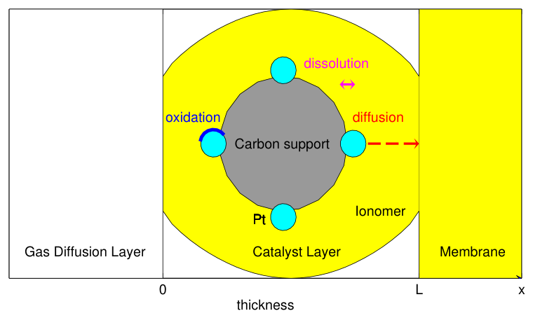
Holby et al. [42] and Li et al. [43] coupled the kinetic model with particle size distribution and approximated it with particle groups. Experimental and theoretical techniques were compared in the work [42] in order to validate the kinetic model. Agravante and Gostick [44], in their review, provided a detailed comparison of Darling–Meyers and Holby–Morgan governing equations, further simplifying assumptions made by the Rinaldo–Stumper–Eikerling model [45] and other models used in the field. Koltsova et al. [46] compared the results of experimental studies. The ECSA loss of the platinum catalyst was found to have a significant impact on overall fuel-cell performance loss. In the simulation [46], the effect of each degradation mechanism on the overall degradation of the platinum catalyst surface of the cathode was studied. See Figure 1 for the schematic illustration of the catalyst degradation process.

This study systematically examines the Holby–Morgan electrochemical model for degradation of a platinum catalyst under cyclic voltammetry from a mathematical point of view. Local sensitivity analysis in Kovtunenko and Karpenko-Jereb [47] and in Karpenko-Jereb and Kovtunenko [48] predicted variance of cycling operating condition, whereas Kovtunenko [49,50] collected feasible domain for model parameters. The normal distribution of Pt particles was treated in Kovtunenko [51], and in another study by the same author [52], the log-normal distribution was implemented, which is in good agreement with experimental data. Industrial protocols of electric potential of square and triangle wave forms with various upper potential levels were applied to the Holby–Morgan model to model the impact of cycling operating conditions on the durability of fuel cells. The existing Holby–Morgan degradation model is well established and widely used. The novelty of this work’s mathematical contribution consists of developing a pseudo-spectral method for highly efficient numerical computation of its discrete counterpart.

In a CL of thickness L (cm), the Holby–Morgan model looks for time-dependent distributions as $x\in [0,L]$ of the platinum ion (${\mathrm{Pt}}^{2+}$) concentration $c(t,x)>0$ (mol/cm³), the platinum (Pt) particle diameter $d(t,x)>0$ (cm), and the ratio of platinum oxide (PtO) coverage $\theta (t,x)\in (0,1)$ (1). It validates the nonlinear system of reaction-diffusion equations [43]

$$\left\{\begin{array}{c}{\displaystyle \frac{\partial c}{\partial t}}-{\epsilon }^{1/2}{D}_{\mathrm{Pt}}{\displaystyle \frac{{\partial }^{2}c}{\partial x^2}}={\displaystyle \frac{\pi N_{\mathrm{Pt}}}{2\epsilon V_{\mathrm{Pt}}}}{d}^2{r}_{\mathrm{dissol}}(c,d,\theta ),\hfill \\ {\displaystyle \frac{\partial d}{\partial t}}=-\Omega r_{\mathrm{dissol}}(c,d,\theta ),\hfill \\ {\displaystyle \frac{\partial \theta }{\partial t}}+{\displaystyle \frac{2\theta }{d}}{\displaystyle \frac{\partial d}{\partial t}}={\displaystyle \frac{1}{\Gamma }}{r}_{\mathrm{oxide}}\left(\theta \right),\hfill \end{array}\right.$$

(1)

where the reaction rates $r_{\mathrm{dissol}}$ (mol/(cm² s)) and $r_{\mathrm{oxide}}$ (mol/(cm² s)) satisfy the following Butler–Volmer equations. The reaction rate of Pt²⁺ dissolution is

$$\left\{\begin{array}{cc}{r}_{\mathrm{dissol}}(c,d,\theta )\hfill & =\Gamma (1-\theta )({\nu }_{1}exp[-{\displaystyle \frac{H_{1,\mathrm{fit}}+(1-{\beta }_1)H_1(d,\theta )}{RT}}]\hfill \\ \hfill & -{\nu }_2{\displaystyle \frac{c}{c_{\mathrm{ref}}}}exp[{\displaystyle \frac{-H_{1,\mathrm{fit}}+{\beta }_1{H}_1(d,\theta )}{RT}}]).\hfill \end{array}\right.$$

(2)

In (2), the molar enthalpy difference for dissolution (J/mol) is

$$H_1(d,\theta )=nF(U_{\mathrm{eq}}-V)-{\displaystyle \frac{4\Omega }{d}}\left({\gamma }_0\left(\theta \right)-\Gamma n_{2}F\theta V\right),$$

(3)

and the surface tension difference (J/cm²) is

$$\left\{\begin{array}{cc}{\gamma }_0\left(\theta \right)\hfill & =\gamma +\Gamma RT\theta (ln[{\displaystyle \frac{{\nu }_2^{★}}{{\nu }_1^{★}}}{10}^{-2pH}]\hfill \\ \hfill & +{\displaystyle \frac{2n_{2}F{U}_{\mathrm{fit}}+\omega \theta }{2RT}}+ln({\displaystyle \frac{\theta }{2}})+{\displaystyle \frac{2-\theta }{\theta }}ln(1-{\displaystyle \frac{\theta }{2}})).\hfill \end{array}\right.$$

(4)

The reaction rate of PtO coverage yields

$$\left\{\begin{array}{cc}{r}_{\mathrm{oxide}}\left(\theta \right)\hfill & =\Gamma ({\nu }_1^{★}(1-{\displaystyle \frac{\theta }{2}})exp[-{\displaystyle \frac{H_{2,\mathrm{fit}}+\lambda \theta +(1-{\beta }_2)H_2\left(\theta \right)}{RT}}]\hfill \\ \hfill & -{\nu }_2^{★}{10}^{-2pH}exp[{\displaystyle \frac{-H_{2,\mathrm{fit}}-\lambda \theta +{\beta }_2{H}_2\left(\theta \right)}{RT}}]),\hfill \end{array}\right.$$

(5)

with the molar enthalpy difference for oxidation (J/mol)

$$H_2\left(\theta \right)=n_{2}F(U_{\mathrm{fit}}-V)+\omega \theta .$$

(6)

The initial conditions are prescribed as

$$c=0,d=d_{\mathrm{Pt}},\theta =0\mathrm{as}t=0,$$

(7)

with a no-flux boundary condition at the left surface and zero at the right surface of the CL:

$${\displaystyle \frac{\partial c}{\partial x}}=0\mathrm{as}x=0,c=0\mathrm{as}x=L.$$

(8)

In the governing relations (1)–(8), R is the gas constant and F is the Faraday constant. The catalyst’s structural and kinetic parameters according to the literature [40,41,42,43] are gathered in

Table 1. The parameters for Pt²⁺ dissolution.

Symbol	Value	Units	Description
${\nu }_1$	$1\times {10}^4$	Hz	dissolution attempt frequency
${\nu }_2$	$8\times {10}^5$	Hz	backward dissolution rate factor
${\beta }_1$	0.5		Butler transfer coefficient for dissolution
n	2		electrons transferred during dissolution
$U_{\mathrm{eq}}$	1.118	V	Pt dissolution bulk equilibrium voltage
$\Omega$	9.09	cm3/mol	molar volume of Pt
$\gamma$	$2.4\times {10}^{-4}$	J/cm2	Pt [1 1 1] surface tension
$c_{\mathrm{ref}}$	1	mol/cm3	reference Pt2+ concentration
$H_{1,\mathrm{fit}}$	$4.4\times {10}^4$	J/mol	partial Pt dissolution activation enthalpy
$D_{\mathrm{Pt}}$	$1\times {10}^{-6}$	cm2/s	diffusion coefficient of Pt2+ in membrane

for Pt²⁺ dissolution and in

Table 2. The parameters for PtO formation.

Symbol	Value	Units	Description
${\nu }_1^{★}$	$1\times {10}^4$	Hz	forward PtO formation rate constant
${\nu }_2^{★}$	$2\times {10}^{-2}$	Hz	backward PtO formation rate constant
$\Gamma$	$2.2\times {10}^{-9}$	mol/cm2	Pt surface site density
${\beta }_2$	0.5		Butler transfer coefficient for oxidation
$n_2$	2		electrons transferred during oxidation
$U_{\mathrm{fit}}$	0.8	V	PtO formation bulk equilibrium voltage
$\lambda$	$2\times {10}^4$	J/mol	PtO dependent kinetic barrier constant
$\omega$	$5\times {10}^4$	J/mol	Pt oxide–oxide interaction energy
$H_{2,\mathrm{fit}}$	$1.2\times {10}^4$	J/mol	partial PtO formation activation enthalpy

for PtO formation, and the key operating parameters are indicated in

Table 3. The parameters of the CL.

Symbol	Value	Units	Description
L	${10}^{-3}$	cm	thickness
T	353.15	K	temperature
$pH$	0		potential of hydrogen
$d_{\mathrm{Pt}}$	$3\times {10}^{-7}$	cm	Pt particle diameter
$V_{\mathrm{Pt}}$	$1.4\times {10}^{-20}$	cm3	Pt particle density
$p_{\mathrm{Pt}}$	$4\times {10}^{-4}$	g/cm2	Pt particle loading
$\epsilon$	0.02		Pt/C volume fraction
${\rho }_{\mathrm{Pt}}$	21.45	g/cm3	Pt particle density
$N_{\mathrm{Pt}}$	$1.3\times {10}^{18}$		Pt particle count

and thereafter.

This study applies an asymmetric square profile for 40 s electric potential $V\left(t\right)$, alternating between voltages of 0.6 (V) for 10 (s) and 0.9 (V) for 30 (s), as recommended by the Fuel Cell and Hydrogen Joint Undertaking (FCH JU).

3. Methods

Advanced space-time discretization of the Holby–Morgan model (1)–(8) is described herein. Let time points $0=t^0<t^1<\dots$ compose intervals of length ${\tau }^l:=t^l-t^{l-1}>0$ as $l=1,2,\dots$. Following time stepping by Ascher et al. [53], implicit–explicit (IMEX) iteration with an intermediate $(l-1/2)$ time step was introduced in Kovtunenko and Karpenko-Jereb [54]:

$$\left\{\begin{array}{c}{c}^{l-1/2}-w{\tau }^l{\epsilon }^{1/2}{D}_{\mathrm{Pt}}{\displaystyle \frac{d^2{c}^{l-1/2}}{d{x}^2}}=c^{l-1}+w{\tau }^l{\displaystyle \frac{\pi N_{\mathrm{Pt}}}{2\epsilon V_{\mathrm{Pt}}}}{\left(d^{l-1}\right)}^2{r}_{\mathrm{dissol}}(c^{l-1},d^{l-1},{\theta }^{l-1}),\hfill \\ c^l=c^{l-1}+{\tau }^l{\epsilon }^{1/2}{D}_{\mathrm{Pt}}{\displaystyle \frac{d^2{c}^{l-1/2}}{d{x}^2}}+{\tau }^l{\displaystyle \frac{\pi N_{\mathrm{Pt}}}{2\epsilon V_{\mathrm{Pt}}}}{\left(d^{l-1}\right)}^2{r}_{\mathrm{dissol}}(c^{l-1/2},d^{l-1},{\theta }^{l-1}),\hfill \\ {\displaystyle \frac{d{c}^{l-1/2}}{dx}}={\displaystyle \frac{d{c}^l}{dx}}=0\mathrm{as}x=0,c^{l-1/2}=c^l=0\mathrm{as}x=L,\hfill \\ d^l=d^{l-1}-{\tau }^l\Omega r_{\mathrm{dissol}}(c^{l-1},d^{l-1},{\theta }^{l-1}),\hfill \\ {\theta }^l={\theta }^{l-1}+{\tau }^l{\displaystyle \frac{2\Omega {\theta }^{l-1}}{d^{l-1}}}{r}_{\mathrm{dissol}}(c^{l-1},d^{l-1},{\theta }^{l-1})+{\tau }^l{\displaystyle \frac{1}{\Gamma }}{r}_{\mathrm{oxide}}\left({\theta }^{l-1}\right),\hfill \end{array}\right.$$

(9)

where the IMEX parameter is set to $w=0.5$ and initialized at $l=0$ with

$$c^0=0,d^0=d_{\mathrm{Pt}},{\theta }^0=0.$$

(10)

To solve the Cauchy problem (9)–(10) with nonlinear reaction terms with respect to $c^l\left(x\right)$, $d^l\left(x\right)$, and ${\theta }^l\left(x\right)$, the 4th-order Runge–Kutta method (RK4) with variable step size ${\tau }^l$ was elaborated in Kovtunenko [55]. For the square-voltage FCG JU profile, the time step is herein set to ${\tau }^l={10}^{-2}$ (s), which is refined locally to ${\tau }^l={10}^{-4}$ (s) when the electric potential takes off from $V=0.6$ (V) to $V=0.9$ (V) at time 10 (s) during each voltage cycle of 40 (s).

Aiming at accurate space approximation, this study applies the Chebyshev–Gauss–Lobatto (CGL) pseudo-spectral collocation method, which may achieve exponential convergence. For a natural number $p\ge 2$, let the CL thickness $[0,L]$ be split by Chebyshev collocation points

$${\xi }_k:=-cos\left({\displaystyle \frac{\pi (k-1)}{p}}\right),x_k:={\displaystyle \frac{L}{2}}\left(1+{\xi }_k\right),k=1,\dots ,p+1,$$

(11)

with end points $x_1=0$ and $x_{p+1}=L$. Lagrange polynomials of degree p

$${\ell }_k^p\left(x\right):={\displaystyle \prod _{k\ne m=1}^p}{\displaystyle \frac{x-x_m}{x_k-x_m}},k=1,\dots ,p+1,$$

(12)

validate the interpolation property

$${\ell }_k^p\left(x_m\right)=\left\{\begin{array}{c}1\mathrm{if}m=k,\hfill \\ 0\mathrm{if}m\ne k.\hfill \end{array}\right.$$

The solution ansatz in the polynomial basis

$$c^l\left(x\right)={\displaystyle \sum _{k=1}^{p+1}}{c}_k^l{\ell }_k^p\left(x\right),d^l\left(x\right)={\displaystyle \sum _{k=1}^{p+1}}{d}_k^l{\ell }_k^p\left(x\right),{\theta }^l\left(x\right)={\displaystyle \sum _{k=1}^{p+1}}{\theta }_k^l{\ell }_k^p\left(x\right)$$

(13)

fully discretizes Equations (9) and (10) in the form

$$\left\{\begin{array}{c}{c}_k^{l-1/2}-w{\tau }^l{\epsilon }^{1/2}{D}_{\mathrm{Pt}}{\displaystyle {\sum }_{n=1}^p}{S}_{kn}{c}_n^{l-1/2}\hfill \\ =c^{l-1}k+w{\tau }^l{\displaystyle \frac{\pi N_{\mathrm{Pt}}}{2\epsilon V_{\mathrm{Pt}}}}{\left(d_k^{l-1}\right)}^2{r}_{\mathrm{dissol}}(c_k^{l-1},d_k^{l-1},{\theta }_k^{l-1}),c_{p+1}^{l-1/2}=0,\hfill \\ c_k^l=c_k^{l-1}+{\tau }^l{\epsilon }^{1/2}{\displaystyle {\sum }_{n=1}^p}{S}_{kn}{c}_n^{l-1/2}\hfill \\ +{\tau }^l{\displaystyle \frac{\pi N_{\mathrm{Pt}}}{2\epsilon V_{\mathrm{Pt}}}}{\left(d_k^{l-1}\right)}^2{r}_{\mathrm{dissol}}(c_k^{l-1/2},d_k^{l-1},{\theta }_k^{l-1}),c_{p+1}^l=0,\hfill \\ d_k^l=d_k^{l-1}-{\tau }^l\Omega r_{\mathrm{dissol}}(c_k^{l-1},d_k^{l-1},{\theta }_k^{l-1}),\hfill \\ {\theta }_k^l={\theta }_k^{l-1}+{\tau }^l{\displaystyle \frac{2\Omega {\theta }_k^{l-1}}{d_k^{l-1}}}{r}_{\mathrm{dissol}}(c_k^{l-1},d_k^{l-1},{\theta }_k^{l-1})+{\tau }^l{\displaystyle \frac{1}{\Gamma }}{r}_{\mathrm{oxide}}\left({\theta }_k^{l-1}\right),\hfill \end{array}\right.$$

(14)

subjected to the initial condition

$$c_k^0=0,d_k^0=d_{\mathrm{Pt}},{\theta }_k^0=0.$$

(15)

In (14), the stiffness matrix

$$S_{kn}:={\displaystyle \sum _{m=2}^{p+1}}{D}_{km}{D}_{mn}$$

(16)

is built from the matrix of derivatives (see Gheorghiu [56])

$$D_{mn}:={\displaystyle \frac{2}{L}}\left\{\begin{array}{cc}{\displaystyle \frac{{\alpha }_m}{{\alpha }_n}}{\displaystyle \frac{{(-1)}^{m+n}}{{\xi }_m+{\xi }_n}}\hfill & \mathrm{if}m\ne n,\hfill \\ -{\displaystyle \frac{{\xi }_m}{2{(1-{\xi }_m)}^2}}\hfill & \mathrm{if}m=n=2,\dots ,p,\hfill \\ {\displaystyle \frac{2p^2+1}{6}}\hfill & \mathrm{if}m=n=1,\hfill \\ -{\displaystyle \frac{2p^2+1}{6}}\hfill & \mathrm{if}m=n=p+1\hfill \end{array}\right.$$

(17)

where ${\alpha }_m=1$ as $m=2,\dots ,p$, and ${\alpha }_1={\alpha }_{p+1}=1$. The Neumann boundary conditions at $x_1=0$ are incorporated in S by means of the identities

$${\displaystyle \sum _{n=1}^{p+1}}{D}_{1n}{c}_n^{l-1/2}=0,{\displaystyle \sum _{n=1}^{p+1}}{D}_{1n}{c}_n^l=0.$$

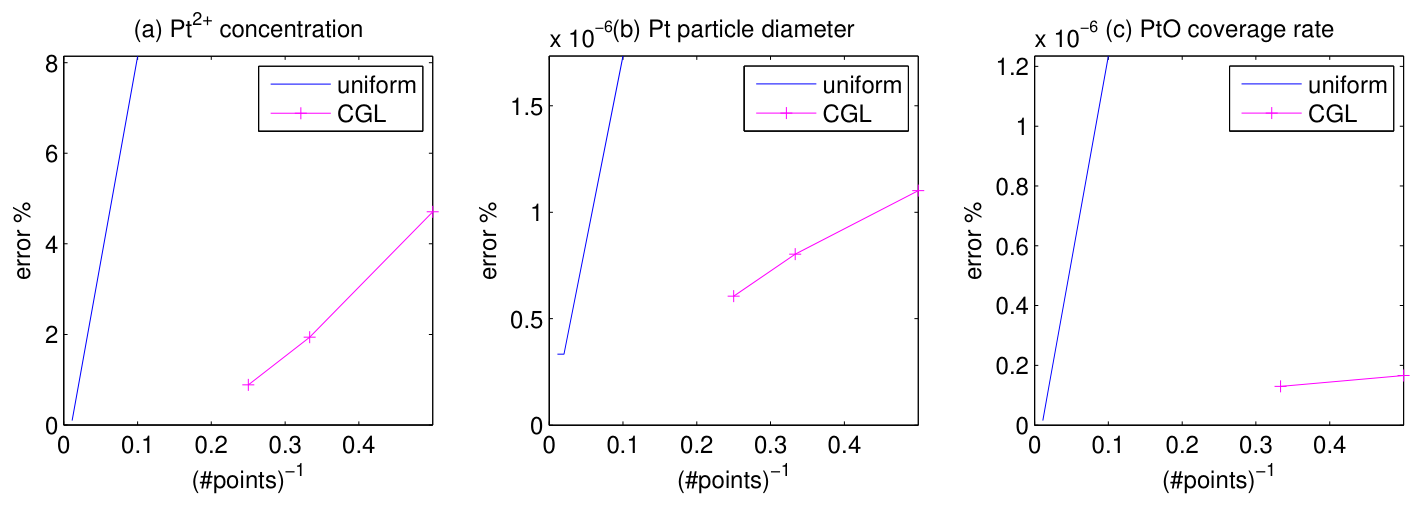
To test the accuracy of the CGL approximation, (11)–(17), it is herein compared with uniform meshing of the CL thickness by $N+1$ points with equal spacing $h:=L/N$. The maximum error during $l=1,\dots ,4037$ time steps within one voltage cycle, measured as a percentage with respect to the finest mesh of $N=100$, is depicted in Figure 2 versus the reciprocal of the number of points (#points). The errors in Pt²⁺ concentration c, Pt particle diameter d, and PtO coverage ratio $\theta$ are shown through respective plots (a)–(c). There, one line represents uniform meshing by $N=10,\dots ,90$ (that is (#points)⁻¹ = 1/N), and another line is obtained for Chebyshev collocation points as $p=2,3,4$ (that is, (#points)⁻¹ = 1/p). Whereas the error in Figure 2b,c is negligible, one concludes from Figure 2a that the 8% threshold for $N+1=11$ of uniform points, which was used in our previous works, is easily improved by only $p+1=3$ of collocation points. Correspondingly, the accuracy for $N+1=101$ uniform points is attained by the use $p+1=5$ CGL basis polynomials.

For convenience, selected numerical values of the error are collected in

Table 4. Maximum error within voltage cycle for uniform meshing and for CGL collocation.

#Points	(#Points)−1	Error c (%)	Error d (%)	Error $\mathit{\theta }$ (%)
$N=10$	$1/N=0.1$	8.14	$1.73\times {10}^{-6}$	$1.23\times {10}^{-6}$
$N=50$	$1/N=0.02$	0.89	$3.33\times {10}^{-7}$	$1.37\times {10}^{-7}$
$N=90$	$1/N=0.01$	0.09	$3.33\times {10}^{-7}$	$1.52\times {10}^{-7}$
$p=2$	$1/p=0.5$	4.7	$1.1\times {10}^{-6}$	$1.65\times {10}^{-7}$
$p=3$	$1/p=0.33$	1.93	$8.03\times {10}^{-7}$	$1.29\times {10}^{-7}$
$p=4$	$1/p=0.25$	0.88	$6.05\times {10}^{-7}$	$1.37\times {10}^{-7}$

.

With the help of (11)–(13), it is possible to approximate the weighted integral mean

$${\tilde{c}}^l:={\int }_0^L{\displaystyle \frac{c^l\left(x\right)dx,}{\pi \sqrt{1-{\left(\frac{2}{L}x-1\right)}^2}}}{\tilde{d}}^l:={\int }_0^L{\displaystyle \frac{d^l\left(x\right)dx}{\pi \sqrt{1-{\left(\frac{2}{L}x-1\right)}^2}}},{\tilde{\theta }}^l:={\int }_0^L{\displaystyle \frac{{\theta }^l\left(x\right)dx}{\pi \sqrt{1-{\left(\frac{2}{L}x-1\right)}^2}}}$$

as the CGL quadrature

$${\tilde{c}}^l={\displaystyle \sum _{k=1}^{p+1}}{w}_k{c}_k^l,{\tilde{d}}^l={\displaystyle \sum _{k=1}^{p+1}}{w}_k{d}_k^l,{\tilde{\theta }}^l={\displaystyle \sum _{k=1}^{p+1}}{w}_k{\theta }_k^l,$$

(18)

where the weights are $w_k:=1/\left({\alpha }_{k}p\right)$. These formulas (18) are exact for polynomials of degree $2p+1$ and will be used in the following evaluation.

4. Results

On every time interval $t\in [t^{l-1},t^l]$, let Lagrange interpolation polynomials be defined according to (12) as

$${\ell }_1^2\left(t\right):={\displaystyle \frac{t-t^l}{t^{l-1}-t^l}},{\ell }_2^2\left(t\right):={\displaystyle \frac{t-t^{l-1}}{t^l-t^{l-1}}}.$$

(19)

Then, using spatial expansion (13), the solution is interpolated piecewise linearly in time as

$$\left\{\begin{array}{c}c(t,x)={\ell }_1^2\left(t\right)c^{l-1}\left(x\right)+{\ell }_2^2\left(t\right)c^l\left(x\right),\hfill \\ d(t,x)={\ell }_1^2\left(t\right)d^{l-1}\left(x\right)+{\ell }_2^2\left(t\right)d^l\left(x\right),\hfill \\ \theta (t,x)={\ell }_1^2\left(t\right){\theta }^{l-1}\left(x\right)+{\ell }_2^2\left(t\right){\theta }^l\left(x\right).\hfill \end{array}\right.$$

(20)

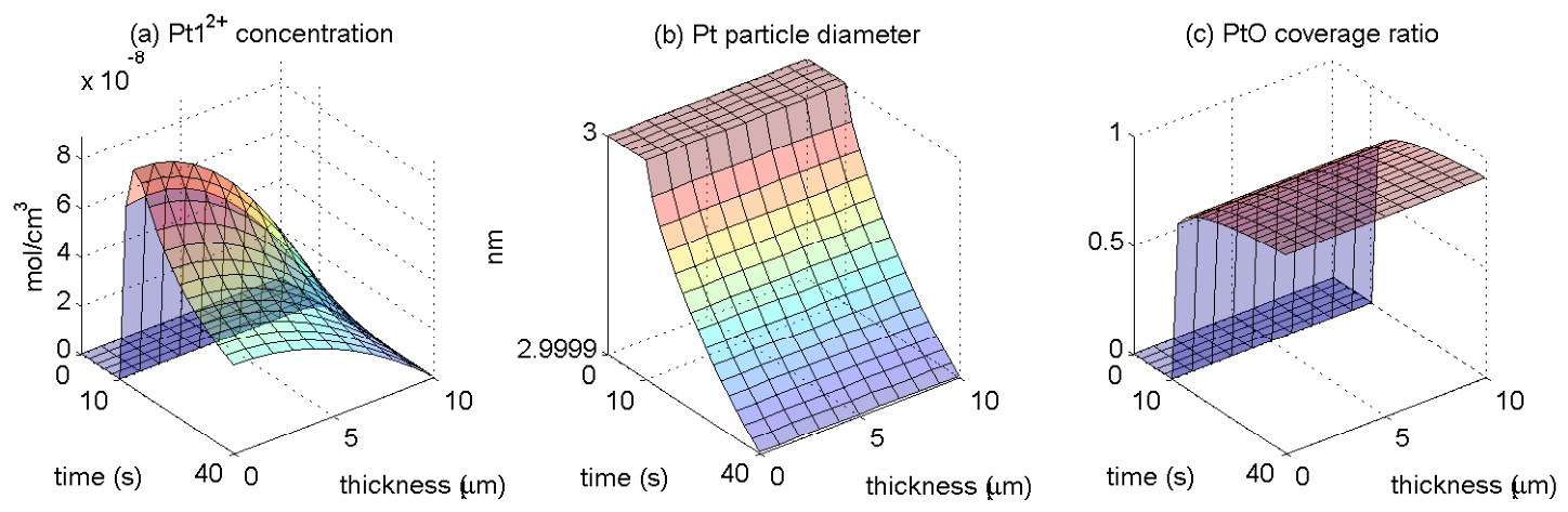
For one voltage cycle, the numerical solution (19)–(20) is presented in Figure 3 as the triple $(c,d,\theta )$. It is depicted versus time $t\in (0,40)$ (s) along the catalyst thickness $x\in (0,10)$, measured in microns (μm). In Figure 3a, the variation in the space variable is observed to be highly significant for Pt²⁺ concentration c due to the diffusion term in the model. Meanwhile, variation along CL is less visible for Pt particle diameter in Figure 3b and PtO coverage ratio in Figure 3c, since d and $\theta$ are affected indirectly by c through the reaction term $r_{\mathrm{dissol}}$.

The weighted integral means over the thickness are defined according to (18) as

$$\left\{\begin{array}{c}\tilde{c}\left(t\right)={\ell }_1^2\left(t\right){\tilde{c}}^{l-1}+{\ell }_2^2\left(t\right){\tilde{c}}^l,\hfill \\ \tilde{d}\left(t\right)={\ell }_1^2\left(t\right){\tilde{d}}^{l-1}+{\ell }_2^2\left(t\right){\tilde{d}}^l,\hfill \\ \tilde{\theta }\left(t\right)={\ell }_1^2\left(t\right){\tilde{\theta }}^{l-1}+{\ell }_2^2\left(t\right){\tilde{\theta }}^l.\hfill \end{array}\right.$$

(21)

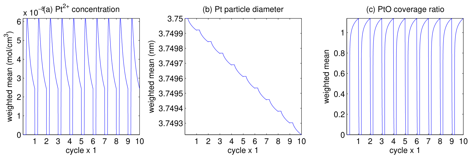
For 10 cycles during $6.\overline{6}$ (min), we depict the respective $(\tilde{c},\tilde{d},\tilde{\theta })$ from (21) in Figure 4 for $l=1,\dots ,$ 40,370 time steps. The Pt²⁺ concentration $c\left(t\right)$ in Figure 4a and PtO coverage ratio $\theta \left(t\right)$ in Figure 4c oscillate periodically between zero and some positive value. In contrast, the Pt particle diameter $d\left(t\right)$ in Figure 4b demonstrates a steady decrease over time with small oscillations.

Furthermore, degradation under AST cycling is investigated in terms of the Pt particle diameter d, electrochemical surface area

$$ECSA:=0.63{\displaystyle \frac{\pi N_{\mathrm{Pt}}}{2}}{d}^2,$$

where the rescaling parameter is derived from experimental data to adjust a model geometric surface area, measured by transmission electron microscopy, to experimental ECSA, measured by cyclic voltammetry (see [42]) and Pt mass

$$m:={\displaystyle \frac{\pi }{6}}{d}^3.$$

We measure the relative loss ratio with respect to initial value at $t=0$ using the weighted integral mean defined by the CGL quadrature (18) such that

$$d_{\mathrm{rat}}\left(t\right):={\displaystyle \frac{\tilde{d}\left(t\right)}{\tilde{d}\left(0\right)}},E_{\mathrm{rat}}\left(t\right):={\displaystyle \frac{\widetilde{ECSA}\left(t\right)}{\widetilde{ECSA}\left(0\right)}}=d_{\mathrm{rat}}^2\left(t\right),m_{\mathrm{rat}}\left(t\right):={\displaystyle \frac{\tilde{m}\left(t\right)}{\tilde{m}\left(0\right)}}=d_{\mathrm{rat}}^3\left(t\right).$$

(22)

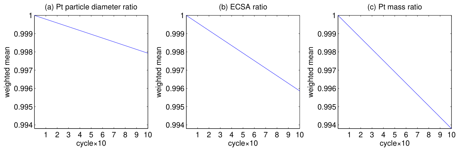
For 100 cycles during $1.\overline{1}$ (h), the ratios $(d_{\mathrm{rat}},E_{\mathrm{rat}},m_{\mathrm{rat}})$ from (22) are presented in Figure 5a–c for 403,700 time steps. Here, small oscillations for each cycle become invisible along the decaying curves. It is evident that $d_{\mathrm{rat}}$ has the lowest loss rate and $m_{\mathrm{rat}}$ the highest loss rate over time.

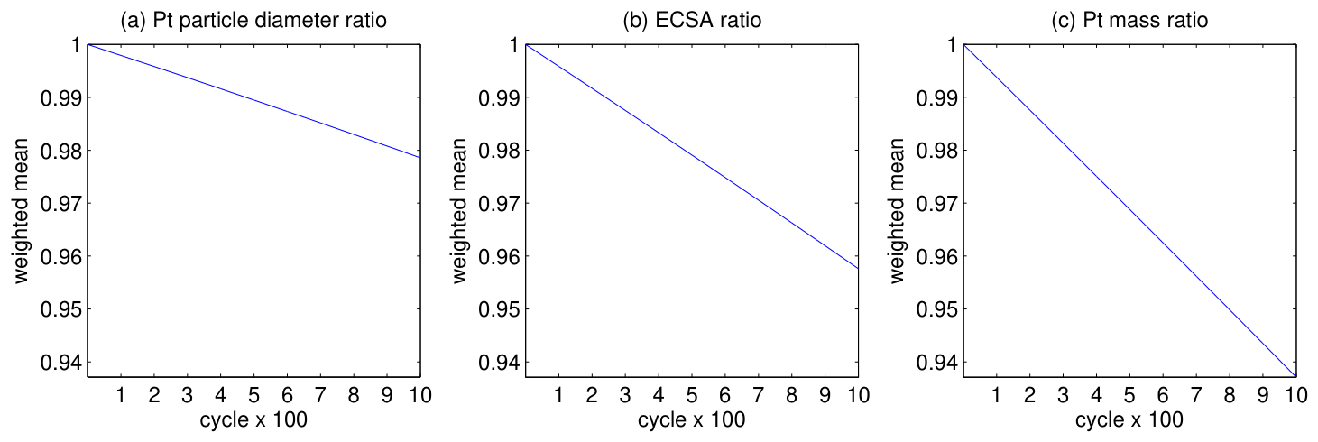
Similarly, for 1000 cycles during $11.\overline{1}$ (h) of AST, time-dependent values of $(d_{\mathrm{rat}},E_{\mathrm{rat}},m_{\mathrm{rat}})$ are shown in Figure 6a–c for 4,037,000 steps. Both Figure 5 and Figure 6 illustrate a linear degradation for all the physical quantities starting at a value of one as $t=0$. Thus, electrochemical degradation in the early stage is dominated by dissolution of small platinum particles. If it continued in this way, then the Pt mass ratio would reach zero in about 15.5 thousand potential cycles.

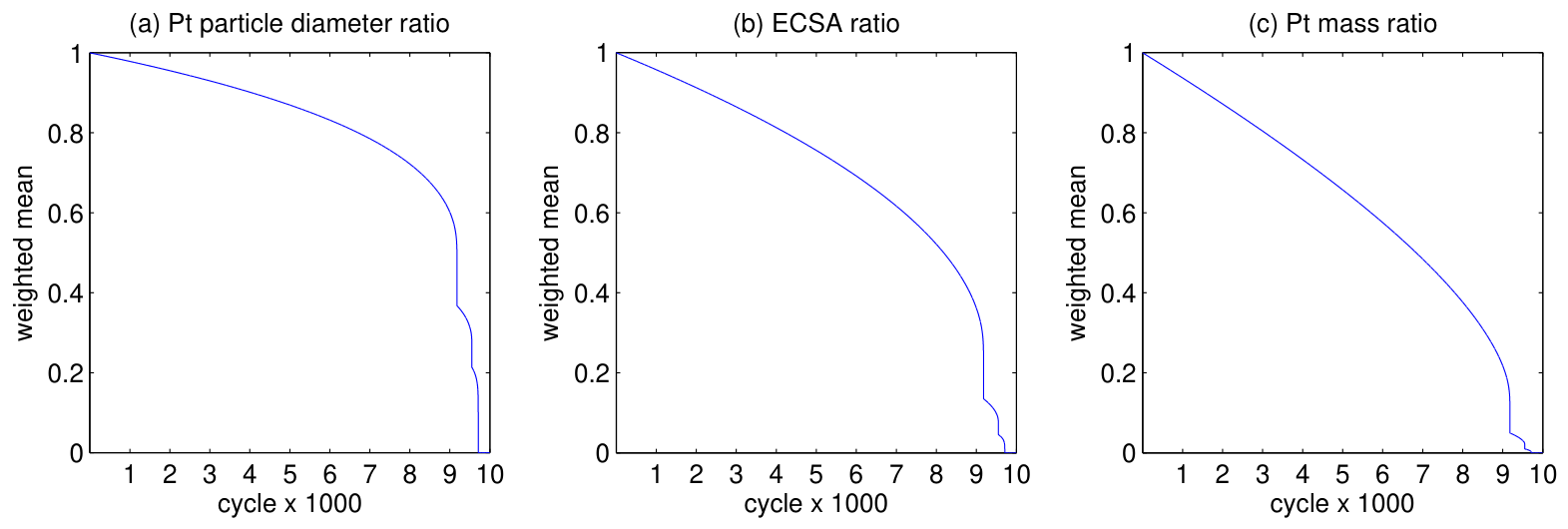
The above behaviour changes dramatically to a nonlinear degradation when AST testing is continued for 10,000 cycles during $111.\overline{1}$ (h), that is, $l=1,\dots ,$ 40,370,000 time steps. Transition toward the nonlinear phase is likely governed by coarsening of platinum nano-particles due to Ostwald ripening and coalescence mechanisms. In

Table 5. Losses of physical quantities and loss rates over ten thousand cycles.

#Cycles	${\mathit{d}}_{\mathbf{rat}}$	${\mathit{d}}_{\mathbf{rat}}^{\prime }$	${\mathit{E}}_{\mathbf{rat}}$	${\mathit{E}}_{\mathbf{rat}}^{\prime }$	${\mathit{m}}_{\mathbf{rat}}$	${\mathit{m}}_{\mathbf{rat}}^{\prime }$
1000	0.98	0.22	0.96	0.43	0.94	0.64
2000	0.95	0.24	0.91	0.46	0.87	0.66
3000	0.93	0.26	0.86	0.49	0.80	0.69
4000	0.90	0.29	0.81	0.54	0.73	0.73
5000	0.87	0.34	0.75	0.59	0.66	0.78
6000	0.83	0.40	0.69	0.68	0.57	0.85
7000	0.78	0.52	0.61	0.82	0.48	0.97
8000	0.72	0.75	0.52	1.10	0.37	1.20
9000	0.60	2.04	0.36	2.50	0.51	2.30

, we collect selected values of losses $(d_{\mathrm{rat}},E_{\mathrm{rat}},m_{\mathrm{rat}})$ together with the loss rates $(d_{\mathrm{rat}}^{\prime },E_{\mathrm{rat}}^{\prime },m_{\mathrm{rat}}^{\prime })$ given per ten thousand cycles (that is, times ${10}^{-4}$ per cycle).

The corresponding curves $(d_{\mathrm{rat}},E_{\mathrm{rat}},m_{\mathrm{rat}})$ depicted in Figure 7a–c start to fall sharply after about 90,000 voltage cycles (that is, 100 h). At this moment, Pt diameter has decreased by 40%, ECSA by 64%, and Pt mass by 49% from the initial values. In this respect, it is worth remembering the quadratic relationship from (22) for the surface area $E_{\mathrm{rat}}$ in plot (b) and the cubic relationship for the mass $m_{\mathrm{rat}}$ in plot (c) with respect to the particle size $d_{\mathrm{rat}}$ given in plot (a). The 1D model assumes spatially homogeneous electrokinetic rates such that all quantities of interest change along one dimension across the catalyst only and remain unchangeable in other directions. Across the CL’s thickness, the degradation is stronger at the right surface $x=L$, where the catalyst matches the membrane due to hydrogen and oxygen crossover. At this end the boundary condition $c=0$ is imposed, and we observe first that $d=0$ after 92,000 cycles. Then the quantities continue to fall toward the CL left surface $x=0$ matching gas diffusion layer such that its weighted integral means are zero. Approximately at 96,000 cycles the weighted integral mean of Pt2+ concentration $\tilde{c}$ becomes close to zero, thereafter the weighted integral mean of Pt particle diameter $\tilde{d}$ falls zero at about 98,000 cycles. To this end CL fully loses its operating capability.

5. Discussion

Degradation processes in fuel cells can be studied using both experiments and simulations. Computer models are cost-effective, with simplified 0D or 1D models often being used, and they involve theoretical hypotheses regarding degradation mechanisms.

Numerical simulation of catalysts is particularly beneficial, owing to their small thickness and complex assembly processes for experimental monitoring of internal electrochemical phenomena. Agravante and Gostick [57] developed a novel approach to platinum degradation using a pore network generating a 2D artificial image of the cathode CL. To predict spatially distributed cell states with high computational efficiency, Altmann et al. [58] presented a quasi-2D time-dependent multi-phase model. Through laboratory experiments, Raga et al. [59] validated a 3D numerical model that characterizes the degradation mechanisms of carbon support corrosion, platinum and carbon oxidation, as well as proton conductivity loss due to acid washout in the membrane of a high-temperature PEMFC. Aiming at further reduction of testing duration regardless of the application case, Thiele et al. [60] proposed an optimization method to generate optimal parameters for realistic testing based on automotive driving cycles.

Inhomogeneous catalytic systems stem from a wide range of chemical synthesis coupling surface kinetics with mass transport, which may occur at different time and length scales. Mathematically, this implies systems of PDE with highly nonlinear reactions or boundary conditions imposed by the surface chemistry. Solving numerically stiff problems by the conventional Computational Fluid Dynamic (CFD) methods involves huge computational costs. Qureshi et al. [61] presented a reduced approach achieved by a low-order asymptotic expansion with respect to the catalyst characteristic size and demonstrated it for a 2D channel flow. The idea behind the order reduction is relevant to minimizing the error of basis functions for solutions.

Spectral methods, finite difference methods, and finite element methods are the main discretization techniques suitable for simulation of stationary and evolutionary differential equations on computers. The reader can find key ideas regarding spectral methods and their programming in MATLAB version 5.3 in the handbook by Trefethen [62]. For spectral points, the roots or extrema of Chebyshev polynomials are commonly used (see Tchébychew [63]). The pseudo-spectral collocation method typically approximates a solution expressed in terms of Lagrange basis polynomials. Schillinger et al. [64] demonstrated that collocation is significantly less expensive than standard Galerkin finite element methods.

Aghdam et al. [65] developed a numerical scheme for discretization of the diffusion equation of fractional order. After time stepping by compact finite differences, the spatial fractional derivative is approximated by the collocation method using Chebyshev polynomials of the fourth kind as test and trial function basis. To demonstrate the performance of different spectral collocation schemes, Nova et al. [66] considered collocation points generated from Gauss–Lobatto nodes; roots of Chebyshev polynomials of the first kind; roots of Legendre polynomials; and equally spaced nodes over the space domain. Supported by time-discrete stability and convergence analysis, numerical examples illustrate the high performance and accuracy of the Chebyshev pseudo-spectral collocation method for representation of integer- and fractional-order diffusion.

6. Conclusions

This study investigated the one-dimensional Holby–Morgan model of electrochemical degradation of platinum in a carbon cathodic catalyst in a proton exchange membrane fuel cell with respect to its lifetime.

A harmonized testing protocol with an asymmetric square-wave potential profile, which is recommended by the European Union, was applied for durability test under accelerated stress cycling. Ion diffusion drives platinum degradation by re-deposition of nano-particles dissolved from the cathode onto larger particles (commonly called Ostwald ripening) and by platinum band formation. This paper aimed to achieve a good approximation of spatial distribution for all physical quantities that change across the catalyst thickness due to diffusion phenomena. Diffusivity is involved in the model directly through platinum ion concentration as well as indirectly through dissolution reaction.

To simulate numerically the long-term behaviour of the platinum catalyst, this study introduced into consideration a highly accurate Chebyshev–Gauss–Lobatto method, which is of the pseudo-spectral collocation type. The spatial approximation attained an error threshold of about 5% by the use of only three Lagrange polynomials on three Chebyshev collocation points. For time stepping, this study employed an advanced implicit–explicit discretization with intermediate time steps incorporated into the standard fourth-order Runge–Kutta method. The efficient discretization makes it possible to overcome the linear degradation within 1000 voltage cycles obtained in previous works, as well as to achieve nonlinear degradation in 10,000 cycles over more than 100 h. In fact, the degradation curve of platinum particle diameter and, consequently, electrochemical surface area over time falls sharply against zero until operating capability is lost.

References

1. Basile, A.; Gupta, R.; Veziroǧlu, T. Compendium of Hydrogen Energy: Hydrogen Storage, Distribution and Infrastructure; Woodhead Publishing: Sawston, UK, 2016. [Google Scholar]
2. Eikerling, M.; Kulikovsky, A. Polymer Electrolyte Fuel Cells; Elsevier: Amsterdam, The Netherlands, 2017. [Google Scholar]
3. Hacker, V.; Mitsushima, S. Fuel Cells and Hydrogen; Elsevier: Amsterdam, The Netherlands, 2018. [Google Scholar] [CrossRef]
4. Hidayat, E.F.; Juliandri; Zain, S.M.; Noviyanti, A.R. Advances in proton exchange membrane fuel cell (PEMFC) materials: A review of developments from 2021 to 2025. J. Power Sources 2025, 657, 238124. [Google Scholar] [CrossRef]
5. Yang, Y.; Yang, L.; Zhang, Q.; Li, Y.; Cao, L.; Li, Q.; Fu, C.; Sheng, C.; Zhang, S.; Xie, H.; et al. Fe-N4 single-atom nitrogen doped carbon catalyst: Dual-functional design for PMS-activated antibiotic degradation and efficient oxygen reduction reaction. Chem. Eng. J. 2026, 527, 171819. [Google Scholar] [CrossRef]
6. Prijatelj, M.; Kregar, A.; Kravos, A.; Katrašnik, T. Modeling core-shell Pt-Co catalyst degradation in fuel cells using a continuum approach. ChemElectroChem. 2025, 12, e202500055. [Google Scholar] [CrossRef]
7. Shih, K.Y.; Chen, Z.M. Microwave-assisted synthesis of graphene-supported PtFeCu nanoparticles for enhanced methanol oxidation in direct methanol fuel cells. J. Nanopart. Res. 2025, 27, 212. [Google Scholar] [CrossRef]
8. Danilov, N.A.; Lei, L.; Medvedev, D.A. Contemporary trends and frontiers in oxygen electrode design for protonic ceramic electrochemical cells: A scientometric perspective. Chem. Eng. J. 2026, 535, 175380. [Google Scholar] [CrossRef]
9. Kumar, A.; Abdullah, M.; Raj, P.B.; Samal, S.K.; Bains, P.S.; Abdul, A.H.; Kaur, G.; Dehghanipour, M. Beyond overpotential: Mechanistic metrics for meaningful electrocatalysis evaluation. J. Alloys Compd. 2026, 1067, 188434. [Google Scholar] [CrossRef]
10. Alimbekova, A.; Daniel, L.; Ihonen, J. Evaluation of double layer capacitance and carbon support corrosion under variable conditions. In 10th Low-Temperature Fuel Cells, Electrolysers & H2 Processing Forum (EFCF 2025); European Fuel Cell Forum AG: Lucerne, Switzerland, 2025; Chapter A1112. [Google Scholar] [CrossRef]
11. Hegde, S.; Wörner, R.; Shabani, B. Automotive PEM fuel cell catalyst layer degradation mechanisms and characterisation techniques, Part II: Platinum degradation. Int. J. Hydrogen Energy 2025, 143, 179–212. [Google Scholar] [CrossRef]
12. Golaghaei, F.; Ahmadi, P.; Ashjaee, M.; Houshfar, E. Mitigation of cathode catalyst degradation in PEM fuel cell hydrogen buses based on the analysis and optimization of driving cycle-associated parameters. Int. J. Hydrogen Energy 2026, 213, 153280. [Google Scholar] [CrossRef]
13. Wang, Z.; Zhang, F.; Wang, B.; Fan, L.; Tongsh, C.; Wu, S.; Ren, H.; Liu, J.; Deng, H.; Du, Q.; et al. Complex causality behind low-Pt-loading cathode degradation in proton exchange membrane fuel cells. Energy 2025, 334, 137663. [Google Scholar] [CrossRef]
14. Rašić, D.; Kravos, A.; Katrašnik, T. Predicting the impact of ambient temperature on PEM fuel cell cold start-up catalyst degradation with a multi-domain and multi-scale modeling framework. Energy Convers. Manag. X 2026, 354, 121254. [Google Scholar] [CrossRef]
15. Elgammal, A. Efficiency and energy–emissions optimization of hydrogen–fuel cell power systems using multi-objective PSO strategy for sustainable marine vessel propulsion. Eng. Technol. J. 2025, 10, 8374–8388. [Google Scholar] [CrossRef]
16. Aliberti, P.; Simone, C.; Addesso, P.; De-Piano, G.; Donsí, F.; Galdi, A.; Maritato, L.; Pantani, R.; Pianese, C.; Polverino, P.; et al. Fuel cells in aviation: Challenges to power the future of flight. Energy Convers. Manag. X 2026, 29, 101426. [Google Scholar] [CrossRef]
17. Guzev, M.; Oleinikov, A.; Bormotin, K.; Dolgopolik, O. Multithreaded integrated design of aiframe panel manufacture processes. In Methods and Tools of Parallel Programming Multicomputers. MTPP 2010; Hsu, C., Malyshkin, V., Eds.; Lecture Notes in Computer Science; Springer: Berlin/Heidelberg, Germany, 2010; Volume 6083, pp. 283–292. [Google Scholar] [CrossRef]
18. Al-Mandhari, M.; Ghosh, A. Modelling solar intermittency effects on PEM electrolyser performance & degradation: A comparison of Oman and UK. Energies 2025, 18, 6131. [Google Scholar] [CrossRef]
19. Mundu, M.; Basajja, M.; Kweyu, E.; Ssempewo, J.; Nnamchi, S.; Uti, D.E. Second-order variational analysis of PV–battery energy management using Jacobi equations. Sci. Rep. 2026, 16, 22314. [Google Scholar] [CrossRef] [PubMed]
20. Annin, B.; Volchkov, Y. Nonclassical models of the theory of plates and shells. J. Appl. Mech. Tech. Phy. 2016, 57, 769–776. [Google Scholar] [CrossRef]
21. Khludnev, A. On a 3D elastic body with a thin rigid inclusion. Math. Notes NEFU 2026, 33, 117–127. [Google Scholar] [CrossRef]
22. Popova, T.; Efremov, A. On modeling thin delaminated inclusions with local damage in a two-dimensional elastic body. Lobachevskii J. Math. 2026, 47, 99–108. [Google Scholar] [CrossRef]
23. Xi, S.; Lazarev, N.P.; Nikiforov, D. Corner contact problem for an elastic body with a wedge shaped rigid inclusion. Math. Notes NEFU 2026, 33, 92–107. [Google Scholar] [CrossRef]
24. Leonova, E.; Rudoy, E.; Sazhenkov, S. The homogenized static model of elastic composite reinforced by curvilinear inclusions. Mech. Res. Commun. 2026, 153, 104657. [Google Scholar] [CrossRef]
25. Furtsev, A. The equilibrium problem for a hyperelastic body with a crack crossing the boundary at zero angle. Math. Notes NEFU 2026, 33, 56–72. [Google Scholar] [CrossRef]
26. Itou, H.; Kovtunenko, V.; Rajagopal, K. Well-posedness of the problem of non-penetrating cracks in elastic bodies whose material moduli depend on the mean normal stress. Int. J. Eng. Sci. 2019, 136, 17–25. [Google Scholar] [CrossRef]
27. Bulíček, M.; Burczak, J.; Schwarzacher, S. Well posedness of nonlinear parabolic systems beyond duality. Ann. Inst. H. Poincaré Anal. Non Linéaire 2019, 36, 1467–1500. [Google Scholar] [CrossRef]
28. Alekseev, G.V.; Pukhnachev, V.V. Boundary value problem for the stationary thermal diffusion model with variable coefficients. Dokl. Math. 2025, 526, 3–7. [Google Scholar] [CrossRef]
29. Fellner, K.; Fischer, J.; Kniely, M.; Tang, B.Q. Global renormalised solutions and equilibration of reaction–diffusion systems with nonlinear diffusion. J. Nonlinear Sci. 2023, 33, 66. [Google Scholar] [CrossRef]
30. Argatov, I.I.; Roosen-Runge, F.; Kocherbitov, V.V. Dynamics of post-occlusion water diffusion in stratum corneum. Sci. Rep. 2022, 12, 17957. [Google Scholar] [CrossRef] [PubMed]
31. Recupero, V. A convergence result for a Stefan problem with phase relaxation. Discret. Contin. Dyn. Syst. Ser. S 2023, 16, 3535–3551. [Google Scholar] [CrossRef]
32. Mallikarjunaiah, S.; Bhatta, D. A finite element model for hydro-thermal convective flow in a porous medium: Effects of hydraulic resistivity and thermal diffusivity. arXiv 2024, arXiv:2402.15917. [Google Scholar] [CrossRef]
33. Jüngel, A.; Massimini, A. Analysis of a Poisson–Nerns–Planck–Fermi system for charge transport in ion channels. J. Differ. Equ. 2024, 395, 38–68. [Google Scholar] [CrossRef]
34. Chok, J.; Petzinna, D. Constrained Dikin–Langevin diffusion for polyhedra. IMA J. Appl. Math. 2026, 91, 210–228. [Google Scholar] [CrossRef]
35. Fellner, K.; Kovtunenko, V.A. A singularly perturbed nonlinear Poisson–Boltzmann equation: Uniform and super-asymptotic expansions. Math. Meth. Appl. Sci. 2015, 38, 3575–3586. [Google Scholar] [CrossRef]
36. Fellner, K.; Kovtunenko, V.A. A discontinuous Poisson–Boltzmann equation with interfacial transfer: Homogenisation and residual error estimate. Appl. Anal. 2016, 95, 2661–2682. [Google Scholar] [CrossRef] [PubMed]
37. Efendiev, M.; Vougalter, V. The preservation of nonnegativity of solutions of a parabolic system with the cubed Laplacian. arXiv 2025. [Google Scholar] [CrossRef]
38. Kovtunenko, V.; Zubkova, A. Mathematical modeling of a discontinuous solution of the generalized Poisson–Nernst–Planck problem in a two-phase medium. Kinet. Relat. Mod. 2018, 11, 119–135. [Google Scholar] [CrossRef]
39. Mickens, R.E. Nonstandard Finite Difference Models of Differential Equations; World Scientific: Singapore, 1994. [Google Scholar] [CrossRef]
40. Darling, R.; Meyers, J. Kinetic model of platinum dissolution in PEMFCs. J. Electrochem. Soc. 2003, 150, A1523–A1527. [Google Scholar] [CrossRef]
41. Holby, E.; Morgan, D. Application of Pt nanoparticle dissolution and oxidation modeling to understanding degradation in PEM fuel cells. J. Electrochem. Soc. 2012, 159, B578–B591. [Google Scholar] [CrossRef]
42. Holby, E.; Sheng, W.; Shao-Horn, Y.; Morgan, D. Pt nanoparticle stability in PEM fuel cells: Influence of particle size distribution and crossover hydrogen. Energy Environ. Sci. 2009, 2, 865–871. [Google Scholar] [CrossRef]
43. Li, Y.; Moriyama, K.; Gu, W.; Arisetty, S.; Wang, C. A one-dimensional Pt degradation model for polymer electrolyte fuel cells. J. Electrochem. Soc. 2015, 162, F834–F842. [Google Scholar] [CrossRef]
44. Agravante, G.J.; Gostick, J.T. Physics-based modeling of platinum catalyst dissolution and oxidation in PEM fuel cells: A focused review. J. Electrochem. Soc. 2026, 173, 074507. [Google Scholar] [CrossRef]
45. Rinaldo, S.G.; Stumper, J.; Eikerling, M. Physical theory of platinum nanoparticle dissolution in polymer electrolyte fuel cells. J. Phys. Chem. C 2010, 114, 5773–5785. [Google Scholar] [CrossRef]
46. Koltsova, E.; Vasilenko, V.; Zhensa, A.; Bogdanovskaya, V.; Radina, M. Mechanism of degradation of polymer fuel cell cathode catalyst: Research and modeling. Theor. Found. Chem. Eng. 2024, 58, 1945–1956. [Google Scholar] [CrossRef]
47. Kovtunenko, V.; Karpenko-Jereb, L. Lifetime of catalyst under voltage cycling in polymer electrolyte fuel cell due to platinum oxidation and dissolution. Technologies 2021, 9, 80. [Google Scholar] [CrossRef]
48. Karpenko-Jereb, L.; Kovtunenko, V. Modeling of the impact of cycling operating conditions on durability of polymer electrolyte fuel cells and its sensitivity analysis. Int. J. Hydrogen Energy 2023, 48, 15646–15656. [Google Scholar] [CrossRef]
49. Kovtunenko, V. The Holby–Morgan model of platinum catalyst degradation in PEM fuel cells: Range of feasible parameters achieved using voltage cycling. Technologies 2023, 11, 184. [Google Scholar] [CrossRef]
50. Kovtunenko, V. Feasible domain of cycling operating conditions and model parameters for Holby–Morgan model of platinum catalyst degradation in PEMFC. Int. J. Hydrogen Energy 2024, 51C, 1518–1526. [Google Scholar] [CrossRef]
51. Kovtunenko, V. Particle size distribution in Holby–Morgan degradation model of platinum on carbon catalyst in fuel cell: Normal distribution. Technologies 2024, 12, 202. [Google Scholar] [CrossRef]
52. Kovtunenko, V. Impact of log-normal particle size distribution in Holby–Morgan degradation model on aging of Pt/C catalyst in PEMFC. Technologies 2025, 13, 262. [Google Scholar] [CrossRef]
53. Ascher, U.; Ruuth, S.; Spiteri, R. Implicit-explicit Runge–Kutta methods for time-dependent partial differential equations. Appl. Numer. Math. 1997, 25, 151–167. [Google Scholar] [CrossRef]
54. Kovtunenko, V.; Karpenko-Jereb, L. Study of voltage cycling conditions on Pt oxidation and dissolution in polymer electrolyte fuel cells. J. Power Sources 2021, 493, 229693. [Google Scholar] [CrossRef]
55. Kovtunenko, V. Variance-based sensitivity analysis of fitting parameters to impact on cycling durability of polymer electrolyte fuel cells. Technologies 2022, 9, 111. [Google Scholar] [CrossRef]
56. Gheorghiu, C.I. Spectral Methods for Differential Problems; Casa Cǎrtii de Stiintǎ: Cluj-Napoca, Romania, 2007. [Google Scholar]
57. Agravante, G.J.; Gostick, J.T. Simulating transient pore-scale behaviour of platinum degradation in PEM fuel cells using pore network modeling. J. Power Sources 2026, 663, 238878. [Google Scholar] [CrossRef]
58. Altmann, F.; Kuzdas, D.; Murschenhofer, D.; Bartlechner, J.; Hametner, C.; Jakubek, S.; Braun, S. A quasi-2D multiphase flow proton exchange membrane fuel cell model for efficient distributed cell state prediction. Energy Convers. Manag. X 2026, 30, 101584. [Google Scholar] [CrossRef]
59. Raga, C.; Montiel, M.; Losantos, R.; Mustata, R.; Valiño, L. Modeling degradation mechanisms of a platinum based catalyst layer in a HT-PEMFC: A 3D numerical study. Int. J. Hydrogen Energy 2024, 83, 51–69. [Google Scholar] [CrossRef]
60. Thiele, P.; Yang, Y.; Liu, Y.; Wick, M.; Pischinger, S. Realistic accelerated stress tests for PEM fuel cells: Validation of load profile optimization via lifetime prognosis in fuel cell electric vehicles. Int. J. Hydrogen Energy 2026, 203, 152594. [Google Scholar] [CrossRef]
61. Qureshi, M.U.; Matera, S.; Runge, D.; Merdon, C.; Fuhrmann, J.; Repke, J.U.; Brösigke, G. Reduced order CFD modeling approach based on the asymptotic expansion—An application for heterogeneous catalytic systems. Chem. Eng. J. 2025, 504, 158684. [Google Scholar] [CrossRef]
62. Trefethen, L.N. Spectral Methods in MATLAB; Software, Environments, and Tools; SIAM: Philadelphia, PA, USA, 2000; Volume 10. [Google Scholar] [CrossRef]
63. Tchébychew, P.L. Théorie des mécanismes connus sous le nom de parallélogrammes. Mém. Savants Étrang. Présentés Á l’Académie St.-Pétersbourg 1853, 7, 539–586. [Google Scholar] [CrossRef]
64. Schillinger, D.; Evans, J.A.; Frischmann, F.; Hiemstra, R.R.; Hsu, M.C.; Hughes, T.J. A collocated C0 finite element method: Reduced quadrature perspective, cost comparison with standard finite elements, and explicit structural dynamics. Int. J. Numer. Methods Eng. 2015, 102, 576–631. [Google Scholar] [CrossRef]
65. Aghdam, Y.E.; Safdari, H.; Azari, Y.; Jafari, H.; Baleanu, D. Numerical investigation of space fractional order diffusion equation by the Chebyshev collocation method of the fourth kind and compact finite difference scheme. Discret. Contin. Dyn. Syst.-S 2021, 14, 2025–2039. [Google Scholar] [CrossRef]
66. Nova, M.H.; Molla, H.U.; Banu, S. Comparison of numerical approximations of one-dimensional space fractional diffusion equation using different types of collocation points in spectral method based on Lagrange’s basis polynomials. Am. J. Comput. Math. 2017, 7, 469–480. [Google Scholar] [CrossRef][Green Version]
Figure 1. Illustration of the catalyst degradation process.
Technologies 14 00462 g001
Figure 2. Maximum error within voltage cycle for Pt2+ concentration c (a), Pt particle diameter d (b), and PtO coverage ratio θ (c) against reciprocal value of #points.
Technologies 14 00462 g002
Figure 3. Solution within 1 cycle: Pt2+ concentration c (a), Pt particle diameter d (b), and PtO coverage ratio θ (c) against time t ( 0 , 40 ) (s) and thickness x ( 0 , 10 ) (μm).
Technologies 14 00462 g003
Figure 4. Weighted integral means within 10 cycles: Pt2+ concentration c (a), Pt particle diameter d (b), and PtO coverage ratio θ (c) against time t ( 0 , 400 ) (s).
Technologies 14 00462 g004
Figure 5. Ratio of weighted integral means within 100 cycles: Pt particle diameter d rat ( t ) (a), ECSA E rat ( t ) (b), and Pt mass m rat ( t ) (c) against time t ( 0 , 4000 ) (s).
Technologies 14 00462 g005
Figure 6. Ratio of weighted integral means within 1000 cycles: Pt particle diameter d rat ( t ) (a), ECSA E rat ( t ) (b), and Pt mass m rat ( t ) (c) against time t (0, 40,000) (s).
Technologies 14 00462 g006
Figure 7. Ratio of weighted integral means within 10,000 cycles: Pt particle diameter d rat ( t ) (a), ECSA E rat ( t ) (b), and Pt mass m rat ( t ) (c) against time t (0, 400,000) (s).
Technologies 14 00462 g007