Probabilistic Assessment of Groundwater Potential Using Spatially Aware Machine Learning and Multimodal Geospatial Data

Abstract

This study presents a spatially aware machine learning model for probabilistic groundwater potential assessment using multimodal geospatial data derived from topography, hydrotopography, climate, soil, land use, Sentinel-1 SAR, and water balance variables. The model incorporates spatially consistent data partitioning, leakage-controlled model development, and probabilistic forecasting to improve the robustness and transferability of groundwater potential assessment. A total of 2402 spatial observations, including 601 groundwater-related locations and 1801 spatially filtered pseudo-absence samples, were used to evaluate eleven machine learning and deep learning models. The proposed hybrid framework achieved the best overall validation results with ROC-AUC of 0.9319, PR-AUC of 0.8363, F1-measure of 0.8226, balanced accuracy of 0.8847, and MCC of 0.7613. Independent spatial block testing further demonstrated strong generalization ability, showing ROC-AUC of 0.9535, PR-AUC of 0.9002, F1-measure of 0.7983, balanced accuracy of 0.8594, and MCC of 0.7336. Comparative experiments demonstrated that the proposed framework remains competitive with state-of-the-art machine learning and deep learning approaches while providing robust probabilistic estimates in spatially separated validation. The resulting groundwater potential maps identify areas with environmental conditions similar to known groundwater observations and provide a reliable basis for prioritizing hydrogeological studies, groundwater exploration, and regional water resources planning in data-poor settings.

1. Introduction

Mapping groundwater potential is a critical task in geoinformation analysis, hydrology, and natural resource management, particularly amid growing water demand, climate variability, and spatial unevenness in water resources [1,2,3]. Groundwater provides a significant share of the water supply for agriculture, industry, and domestic use; however, its spatial distribution is difficult to observe directly, often requiring indirect assessment methods [4,5]. Traditional hydrogeological approaches based on drilling, geophysical surveys, and field measurements are valuable but limited by cost, spatial coverage, and reproducibility [6,7].

In response to these limitations, methods based on geographic information systems and remote sensing are being actively developed. These approaches enable the integration of various data sources, including digital elevation models, climate variables, soil characteristics, land-use information, and satellite observations [8,9,10]. Previous approaches to groundwater potential mapping relied primarily on expert-based weighting schemes in GIS environments. Although such methods are interpretable, their results can be affected by subjectivity and limited reproducibility [11,12]. With the development of open geospatial data and cloud platforms such as Google Earth Engine, it has become possible to build scalable, standardized analytical pipelines for processing large geospatial datasets [13,14].

Meanwhile, machine learning methods, including random forests, gradient boosting, support vector machines, and neural networks, have gained widespread acceptance for modeling complex nonlinear relationships between environmental factors and groundwater-related conditions [15,16,17]. However, despite this progress, many existing studies still primarily focus on algorithm comparison and performance maximization. At the same time, methodological aspects of dataset construction, target interpretation, spatial validation, and leakage monitoring remain understudied [18,19]. A key methodological challenge is correctly formulating the target variable. When mapping groundwater potential, the presence of observations such as springs or wells may be recorded, whereas the absence of such observations does not prove the absence of groundwater. Therefore, pseudo-absence concepts, originally developed in species distribution modeling, are becoming increasingly relevant for this type of problem [20]. However, if pseudo-absence points are incorrectly generated or misinterpreted as true negatives, this can lead to systematic error and an overestimation of model performance [21].

Another important limitation is spatial autocorrelation. Many studies use random splitting into training and test sets, which can result in spatially close observations being placed in both sets. This can artificially inflate the model’s reported accuracy, as nearby locations often have similar environmental conditions [22]. For this reason, spatially sensitive validation strategies, including block and group splits, are needed to assess the model’s generalization ability more realistically [3,17].

Furthermore, data leakage remains a serious but often underestimated challenge in geospatial machine learning. Leakage can occur when a model receives direct or indirect information about the target variable through coordinates, identifiers, distances to known groundwater-related features, or other variables derived from the target variable [18]. Similarly, probability calibration and interpretability are not always sufficiently considered, even though practical groundwater assessment requires not only class separation but also robust probability estimates [19,22]. Thus, existing studies still face several methodological limitations: incorrect interpretation of negative samples, insufficient control for spatial dependence, risk of data leakage, limited reproducibility of workflows, and insufficient attention to probability calibration and interpretability. These limitations highlight the need to shift from algorithm-driven research to systems-oriented and reproducible frameworks.

Beyond groundwater potential mapping, recent studies have highlighted the importance of uncertainty-based groundwater modeling to support robust environmental decision-making. For example, Ref. [23] investigated groundwater flow and contaminant transport under heterogeneous permeability conditions using coupled random field modeling and extended porous media theory. Their results showed that subsurface heterogeneity introduces significant uncertainty into groundwater predictions and emphasized the importance of probabilistic rather than deterministic interpretation of modeling results. Although the objectives differ from groundwater potential assessment, these results reinforce the need for cautious interpretation of spatial prediction models when direct hydrogeological observations are limited.

Computational groundwater models are increasingly viewed as decision support tools rather than a direct replacement for hydrogeological studies. Ref. [24] combined groundwater flow modeling, reactive transport modeling, a genetic algorithm, and finite difference methods to optimize groundwater remediation strategies in complex subsurface conditions. Their study found that computational models are most effective when used to prioritize management actions, while taking into account model uncertainty and the need for independent verification. This view is consistent with the present study, in which probabilistic groundwater suitability maps are intended to support hydrogeological exploration and planning rather than to provide direct evidence of groundwater availability.

To address these challenges, this study proposes a replicable, spatially aware machine learning framework for probabilistic groundwater-related occurrence suitability mapping using multimodal geospatial data. The study does not aim to directly detect or confirm groundwater presence. Instead, it estimates the favorability of environmental conditions associated with known groundwater-related observations. This distinction reflects the indirect nature of remote sensing and geospatial predictors, which characterize environmental conditions rather than subsurface groundwater directly. Groundwater is a subsurface resource that cannot be directly observed using remote sensing or surface-based geospatial data. Therefore, the proposed model should not be interpreted as determining the physical presence or absence of groundwater. Instead, it estimates the likelihood that a location possesses environmental characteristics similar to those associated with documented groundwater-related observations, including springs and wells. These observations are used as indirect indicators of favorable hydrogeological conditions, rather than as direct measurements of groundwater availability.

Existing groundwater potential studies often report high forecast accuracy but pay little attention to whether the claimed performance remains reliable when assessed spatially independently. Furthermore, the construction of pseudo-missing observations and the prevention of information leakage are often poorly documented, complicating the comparison of published results. This study addresses these issues by developing a reproducible groundwater potential assessment workflow that combines spatial block validation, carefully constructed pseudo-missing observations, and multimodal geospatial predictors. The proposed algorithm enables the creation of groundwater potential maps that remain reliable when assessed spatially independently and can be used to prioritize hydrogeological studies, groundwater exploration, and regional water resources management.

The remainder of this paper is organized as follows. Section 2 describes the research area, dataset preparation, feature engineering, and the proposed probabilistic model. Section 3 presents the experimental setup and comparative evaluation of machine learning models, as well as the obtained results. Section 4 discusses the results, methodological aspects, and limitations of the proposed approach. Finally, Section 5 concludes the study and outlines future research directions.

2. Materials and Methods

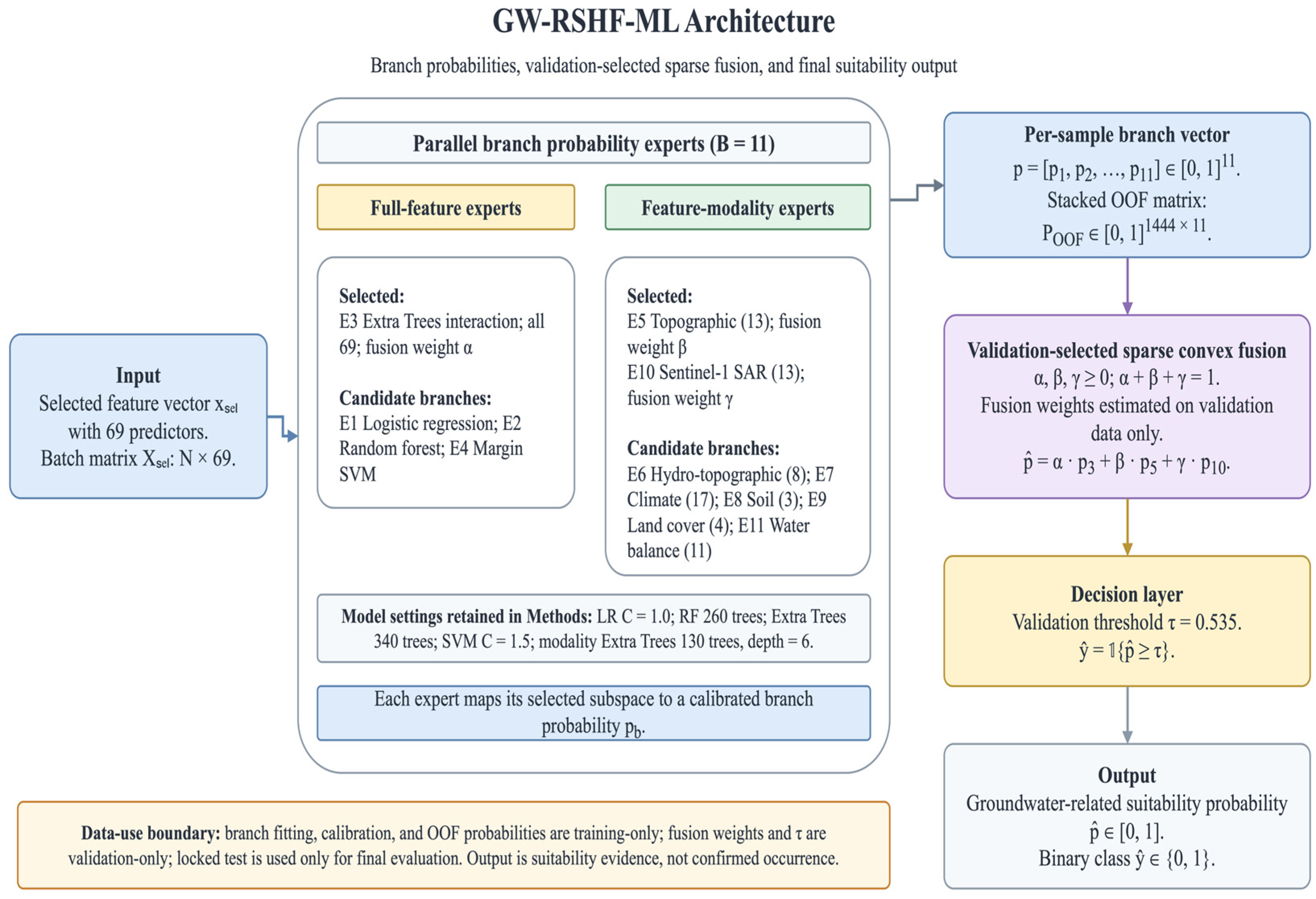
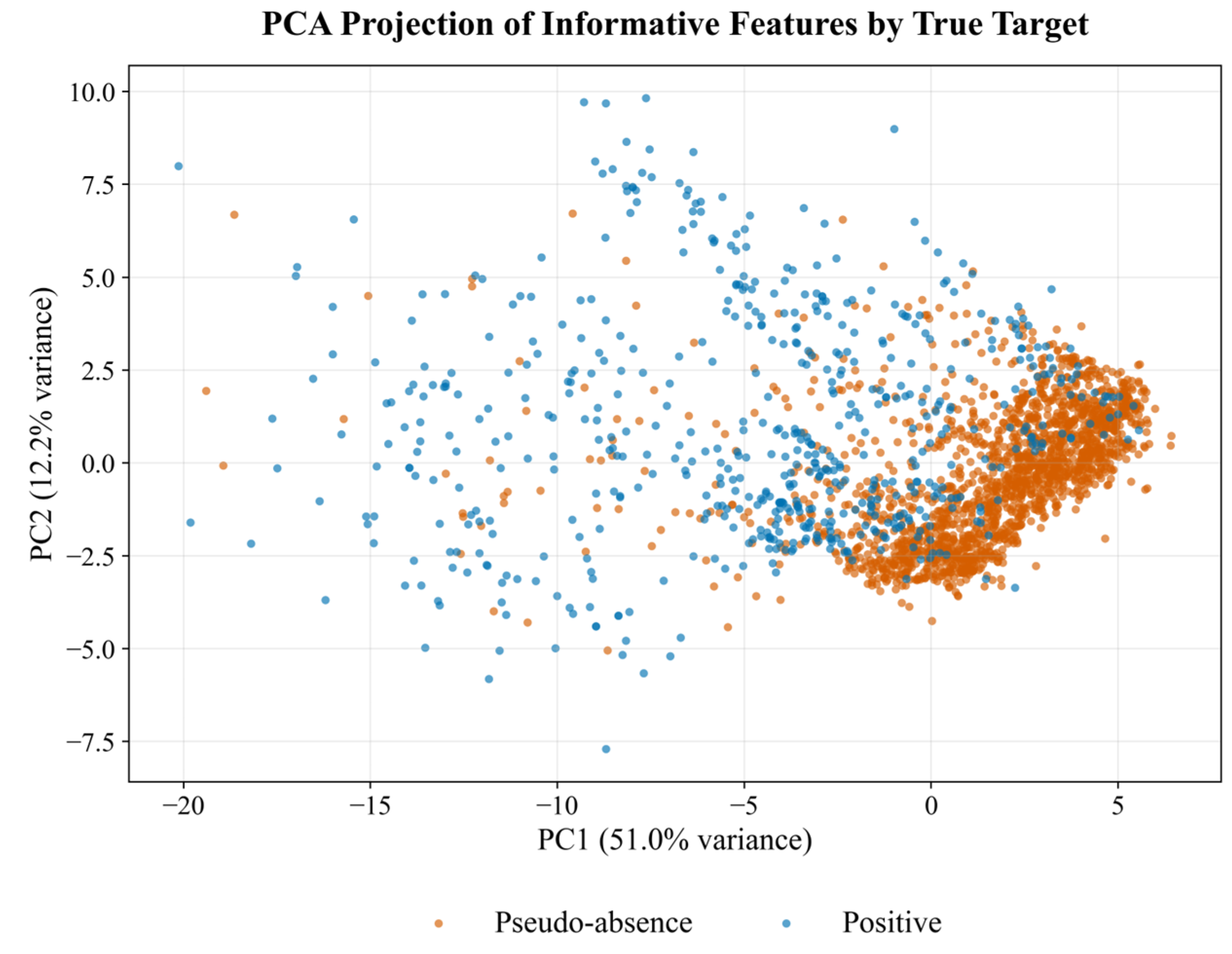
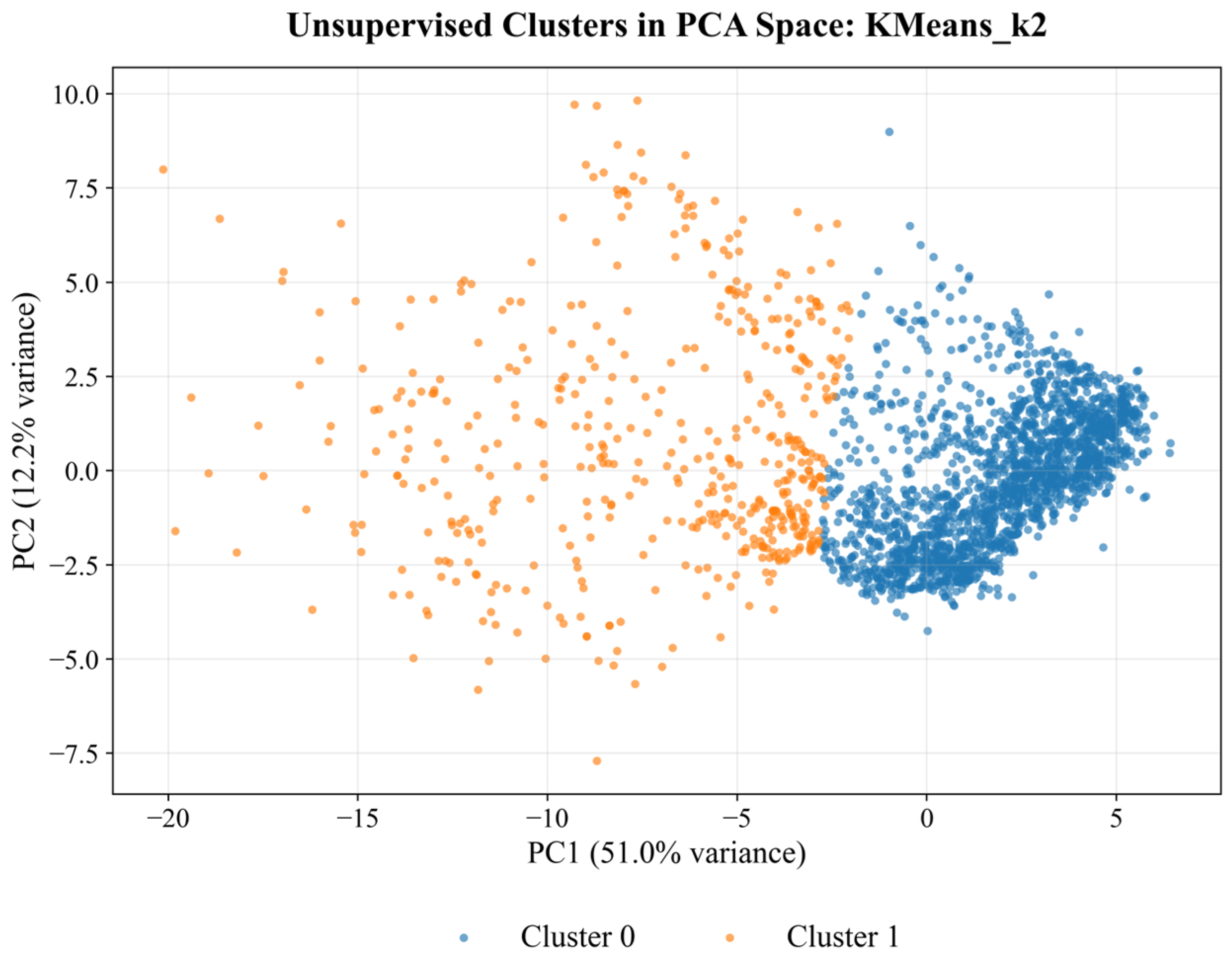
2.1. Preparation and Formation of a Training Geospatial Dataset

Data analysis was structured as a sequential, reproducible workflow to prepare a valid feature space for probabilistic modeling of potentially favorable groundwater distribution zones. The main objective of the data analysis stage was not only to generate a feature table but also to ensure the scientific validity of the sample: eliminating features with the risk of leakage of the target variable, quality control of initial values, checking the class structure, spatial partitioning of the data, and selecting informative variables only from the training set.

The resulting dataset is a point-sampling dataset with supervised learning designed to evaluate whether multimodal geospatial predictors can distinguish documented groundwater-related observations from spatially filtered pseudo-absence locations. Each observation is represented by 89 environmental predictors extracted from independent geospatial layers. Although the initial number of predictors is relatively large compared to the number of observations, feature selection was performed exclusively on the training data, allowing the final predictor set to be reduced to 69 variables before model development. This procedure limits model complexity while retaining only informative environmental predictors.

Table 1. Basic notations used in formalizing the methodology for preparing geospatial data.

№	Designation	Description
1.	$\Omega$	Study area
2.	$p_i$	Spatial observation point
3.	${\lambda }_i$	Point longitude
4.	${\phi }_i$	Point latitude
5.	$y_i$	Target variable
6.	$x_i$	Feature vector for point p_i
7.	$\mathcal{D}$	Final analytical dataset
8.	${\mathcal{F}}_{all}$	Complete set of initial features
9.	${\mathcal{F}}_{model}$	Set of features allowed for modeling
10.	${\mathcal{F}}_{sel}$	Final set of features after train-only selection
11.	$b_i$	Spatial block to which the point belongs
12.	${\mathcal{D}}_{train}$$, {\mathcal{D}}_{valid}$$, {\mathcal{D}}_{test}$	Training, validation, and test datasets.

presents the basic mathematical notations used to formally describe the process of generating and preparing a geospatial dataset. The notations cover the study area, spatial observation points, coordinates, target variable, feature vector, final analytical dataset, feature sets, spatial blocks, and training, validation, and test samples. This table is necessary for a consistent understanding of subsequent formulas and stages of probabilistic modeling of groundwater potential.

The initial sample was formed as a set of two types of spatial points: positive groundwater-related observations and spatially filtered pseudo-absence points. Each point is treated as a geographic observation with coordinates and a target label (1):

$${\mathcal{D}}_{\mathbf{0}}={\left\{\left({\mathit{p}}_{\mathit{i}},{\mathit{y}}_{\mathit{i}}\right)\right\}}_{\mathit{i}=1}^{\mathit{n}},{\mathit{p}}_{\mathit{i}}=\left({\mathit{\lambda }}_{\mathit{i}},{\mathit{\phi }}_{\mathit{i}}\right),{\mathit{y}}_{\mathit{i}}\mathit{\in }\left\{\mathbf{0},\mathbf{1}\right\}$$

(1)

The target variable was defined as follows (2):

$${\mathit{y}}_{\mathit{i}}=\left\{\begin{array}{cc}\mathbf{1},\hfill & \mathrm{if} {\mathit{p}}_{\mathit{i}}\mathit{\in }{\mathcal{S}}^{+}\\ \mathbf{0},\hfill & \mathrm{if} {\mathit{p}}_{\mathit{i}}\mathit{\in }{\mathcal{S}}^{-}\end{array}\right.$$

(2)

where ${\mathcal{S}}^{+}$ is the set of known or probable groundwater-related objects, and ${\mathcal{S}}^{-}$ is the set of filtered pseudo-absence points. The positive class reflects points associated with known groundwater manifestations or objects, such as springs and water wells. The negative class is not interpreted as a proven absence of groundwater. It represents spatially sampled pseudo-absence points used to construct a contrast sample in binary probability modeling. The final class structure after quality control (3):

$$\mathit{\mid }{\mathcal{S}}^{+}\mathit{\mid }=\mathbf{601},\mathit{\mid }{\mathcal{S}}^{-}\mathit{\mid }=\mathbf{1801},\mathit{n}=\mathbf{2402}$$

(3)

This class ratio preserves the real imbalance between known groundwater-related objects and spatially distributed pseudo-absence points but remains suitable for training binary classification models using appropriate quality metrics. The pseudo-absence points were formed not as random points, but as a spatially filtered sample. The main principle was to eliminate obvious intersections with known positive objects and reduce the likelihood of negative points falling in close proximity to groundwater-related observations. Formally, the spatial filtering condition can be written as follows (4):

$${\mathit{p}}_{\mathit{j}}^{-}\in \Omega ,\mathit{d}\left({\mathit{p}}_{\mathit{j}}^{-},{\mathcal{S}}^{+}\right)\ge {\mathit{r}}_{\mathit{min}}$$

(4)

where ${\mathit{p}}_{\mathit{j}}^{-}$ is a pseudo-absence point, $\mathit{d}\left({\mathit{p}}_{\mathit{j}}^{-},{\mathcal{S}}^{+}\right)$ is the minimum distance from this point to the nearest positive observation, and ${\mathit{r}}_{\mathit{m}\mathit{i}\mathit{n}}$ is the minimum spatial filtering buffer. This condition does not prove the absence of groundwater at pseudo-absence points but makes the negative class more appropriate for probabilistic modeling for probabilistic mapping tasks. Therefore, in what follows, the class $\mathit{y}=\mathbf{0}$ is treated as filtered pseudo-absence, and not as confirmed absence. For each point ${\mathit{p}}_{\mathit{i}}$, a feature vector ${\mathbf{x}}_{\mathit{i}}$ was formed, obtained by extracting values from a set of open geospatial layers. These layers described the topographic, hydro-topographic, climatic, soil, landscape, radar, and water-balance characteristics of the territory. The selected predictors were chosen because they represent key environmental factors influencing groundwater availability. Topographic variables describe relief configuration and runoff accumulation, climate variables characterize long-term water availability, soil properties influence infiltration and reservoir capacity, Sentinel-1 SAR data provide information on surface moisture conditions, and water balance indicators reflect regional hydrological processes. Their integration allows for a more comprehensive understanding of environmental conditions associated with groundwater potential. If we denote the set of initial spatial layers as (5):

$$\mathcal{G}=\left\{{\mathit{g}}_{\mathbf{1}},{\mathit{g}}_{\mathbf{2}},\dots ,{\mathit{g}}_{\mathit{m}}\right\}$$

(5)

then the feature vector for each point is defined as (6):

$${\mathbf{x}}_{\mathit{i}}=\left[{\mathit{g}}_{\mathbf{1}}\left({\mathit{p}}_{\mathit{i}}\right),{\mathit{g}}_{\mathbf{2}}\left({\mathit{p}}_{\mathit{i}}\right),\dots ,{\mathit{g}}_{\mathit{m}}\left({\mathit{p}}_{\mathit{i}}\right)\right],\mathit{m}=\mathbf{89}$$

(6)

Thus, each row of the final table corresponds to one spatial point, and each feature column corresponds to the value of a specific geospatial layer or derived indicator at that point. The final initial analytical feature matrix had the form (7):

$${\mathbf{X}}_{\mathit{all}}=\left[\begin{array}{cccc}{\mathit{x}}_{\mathbf{11}}& {\mathit{x}}_{\mathbf{12}}& \dots & {\mathit{x}}_{\mathbf{1}\mathit{m}}\\ {\mathit{x}}_{\mathbf{21}}& {\mathit{x}}_{\mathbf{22}}& \dots & {\mathit{x}}_{\mathbf{2}\mathit{m}}\\ ⋮& ⋮& \ddots & ⋮\\ {\mathit{x}}_{\mathit{n}\mathbf{1}}& {\mathit{x}}_{\mathit{n}\mathbf{2}}& \dots & {\mathit{x}}_{\mathit{n}\mathit{m}}\end{array}\right],\mathit{n}=\mathbf{2402},\mathit{m}=\mathbf{89}$$

(7)

At this stage, it was important that the features were derived from actual source-sampled geospatial layers, not from synthetic fallback values. This increases the reproducibility and scientific validity of further analysis. After generating the source table, quality control of the observations and features was performed. At the row level, the proportion of missing values for each point was analyzed (8):

$${\mathit{M}}_{\mathit{i}}={\displaystyle \frac{\mathbf{1}}{\mathit{m}}}{\displaystyle {{\displaystyle \sum }}_{\mathit{k}=\mathbf{1}}^{\mathit{m}}}\mathit{I}({\mathit{x}}_{\mathit{i}\mathit{k}} \mathrm{is} \mathrm{missing})$$

(8)

where ${\mathit{M}}_{\mathit{i}}$ is the proportion of gaps in the $\mathit{i}$-th row, $\mathit{I}\left(\cdot \right)$ is an indicator function that takes the value 1 when the condition is met and 0 otherwise. Rows with an excessive proportion of gaps were excluded from further analysis (9):

$$\mathcal{D}=\left\{\left({\mathit{p}}_{\mathit{i}},x_{\mathit{i}},{\mathit{y}}_{\mathit{i}}\right):{\mathit{M}}_{\mathit{i}}\le {\mathit{\tau }}_{\mathit{r}\mathit{o}\mathit{w}}\right\}$$

(9)

where ${\mathit{\tau }}_{\mathit{r}\mathit{o}\mathit{w}}$ is the acceptable threshold for missing values at the observation level. After quality control, the final dataset contained (10):

$$\mathcal{D}={\left\{\left({\mathbf{x}}_{\mathit{i}},{\mathit{y}}_{\mathit{i}},{\mathit{b}}_{\mathit{i}}\right)\right\}}_{\mathit{i}=\mathbf{1}}^{\mathbf{2402}}$$

(10)

Additionally, the proportion of omissions for each characteristic was analyzed (11):

$${\mathit{Q}}_{\mathit{k}}={\displaystyle \frac{\mathbf{1}}{\mathit{n}}}{\displaystyle {{\displaystyle \sum }}_{\mathit{i}=\mathbf{1}}^{\mathit{n}}}\mathit{I}({\mathit{x}}_{\mathit{i}\mathit{k}} \mathrm{is} \mathrm{missing})$$

(11)

where ${\mathit{Q}}_{\mathit{k}}$ is the proportion of missing values in the k-th feature. This step allowed us to identify features with potentially low reliability, verify the missingness structure, and prepare the data for subsequent processing without distorting the target variable. One of the key requirements of the analysis was the exclusion of leakage features. Leakage is defined as variables that can directly or indirectly convey information to the model about the target variable, point identifier, coordinates, spatial block, or known groundwater-related objects. The complete set of features was divided into acceptable and unacceptable (12):

$${\mathcal{F}}_{\mathbf{a}\mathbf{l}\mathbf{l}}={\mathcal{F}}_{\mathbf{m}\mathbf{o}\mathbf{d}\mathbf{e}\mathbf{l}}\cup {\mathcal{F}}_{\mathbf{l}\mathbf{e}\mathbf{a}\mathbf{k}},{\mathcal{F}}_{\mathbf{m}\mathbf{o}\mathbf{d}\mathbf{e}\mathbf{l}}\cap {\mathcal{F}}_{\mathbf{l}\mathbf{e}\mathbf{a}\mathbf{k}}=\varnothing$$

(12)

The set of features allowed for modeling was defined as (13):

$${\mathcal{F}}_{\mathit{m}\mathit{o}\mathit{d}\mathit{e}\mathit{l}}={\mathcal{F}}_{\mathit{a}\mathit{l}\mathit{l}}/{\mathcal{F}}_{\mathit{l}\mathit{e}\mathit{a}\mathit{k}}$$

(13)

The ${\mathcal{F}}_{\mathit{l}\mathit{e}\mathit{a}\mathit{k}}$ set included features potentially posing a risk of data leakage: the target variable, observation identifiers, point coordinates, spatial block identifiers, features directly associated with known groundwater/water features, distance variables to target objects, and technical fields that are not independent natural predictors. Excluding these variables is necessary to ensure that the model is trained on physically interpretable characteristics of the area, rather than on service information or technical traces of the sampling process.

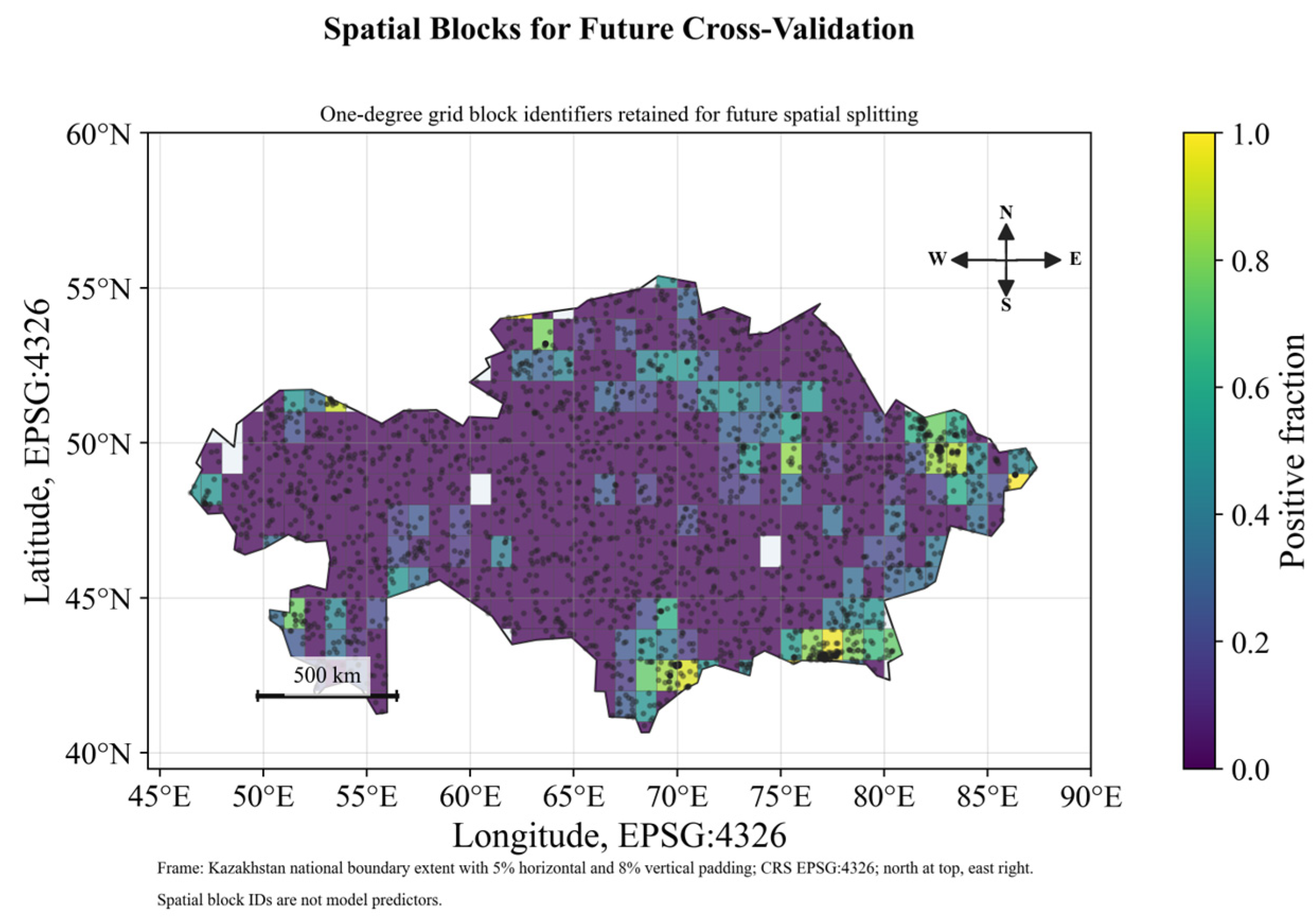
To prevent overestimation of quality, spatial-block grouped partitioning was used. Each point was assigned to a spatial block ${\mathit{b}}_{\mathit{i}}$. The partitioning was performed at the spatial-block level rather than at the level of individual observations, to prevent closely located points with high spatial similarity from being included in both the training and test sets. Formally, this can be represented as follows (14):

$${\mathit{b}}_{\mathit{i}}=\mathit{B}\left({\mathit{p}}_{\mathit{i}}\right)$$

(14)

where $\mathit{B}\left(\cdot \right)$ is the function that assigns a point to a corresponding spatial block. The dataset was then divided into three disjoint parts (15):

$$\mathcal{D}={\mathcal{D}}_{\mathit{t}\mathit{r}\mathit{a}\mathit{i}\mathit{n}}\cup {\mathcal{D}}_{\mathit{v}\mathit{a}\mathit{l}\mathit{i}\mathit{d}}\cup {\mathcal{D}}_{\mathit{t}\mathit{e}\mathit{s}\mathit{t}}$$

(15)

subject to condition (16):

$${\mathcal{D}}_{\mathit{t}\mathit{r}\mathit{a}\mathit{i}\mathit{n}}\cap {\mathcal{D}}_{\mathit{v}\mathit{a}\mathit{l}\mathit{i}\mathit{d}}\cap {\mathcal{D}}_{\mathit{t}\mathit{e}\mathit{s}\mathit{t}}=\varnothing$$

(16)

For spatial blocks, the condition of non-intersection between parts was also met (17):

$${\mathcal{B}}_{\mathbf{t}\mathbf{r}\mathbf{a}\mathbf{i}\mathbf{n}}\cap {\mathcal{B}}_{\mathbf{v}\mathbf{a}\mathbf{l}\mathbf{i}\mathbf{d}}\cap {\mathcal{B}}_{\mathbf{t}\mathbf{e}\mathbf{s}\mathbf{t}}=\varnothing$$

(17)

The actual distribution of observations was as follows (18):

$$\mathbf{\mid }{\mathcal{D}}_{\mathbf{t}\mathbf{r}\mathbf{a}\mathbf{i}\mathbf{n}}\mathbf{\mid }=\mathbf{1444},\mathbf{\mid }{\mathcal{D}}_{\mathbf{v}\mathbf{a}\mathbf{l}\mathbf{i}\mathbf{d}}\mathbf{\mid }=\mathbf{482},\mathbf{\mid }{\mathcal{D}}_{\mathbf{t}\mathbf{e}\mathbf{s}\mathbf{t}}\mathbf{\mid }=\mathbf{476}$$

(18)

Model performance was assessed using the same type of observations, as there is no publicly available, independent, nationwide hydrogeological inventory for Kazakhstan confirming the absence or presence of groundwater. Therefore, validation was conducted on spatially independent subsets of the same dataset, obtained using point sampling, using a block partitioning into training, validation, and test sets. This protocol provides a more realistic assessment of spatial generalization than random partitioning, although it should not be interpreted as independent hydrogeological validation. All preprocessing parameters were evaluated exclusively on the training portion of ${\mathcal{D}}_{\mathit{t}\mathit{r}\mathit{a}\mathit{i}\mathit{n}}$ and then applied to the validation and test portions. This eliminates the transfer of information from validation/test to the training process. For numerical features, a transformation of the form (19) was used:

$${\tilde{\mathit{x}}}_{\mathit{i}\mathit{k}}={\displaystyle \frac{{\mathit{x}}_{\mathit{i}\mathit{k}}-{\mu }_{\mathit{k}}^{\mathit{t}\mathit{r}\mathit{a}\mathit{i}\mathit{n}}}{{\mathit{\sigma }}_{\mathit{k}}^{\mathit{t}\mathit{r}\mathit{a}\mathit{i}\mathit{n}}}}$$

(19)

where ${\mathit{\mu }}_{\mathit{k}}^{\mathit{t}\mathit{r}\mathit{a}\mathit{i}\mathit{n}}$ and ${\mathit{\sigma }}_{\mathit{k}}^{\mathit{t}\mathit{r}\mathit{a}\mathit{i}\mathit{n}}$ are the mean and standard deviation of the $\mathit{k}$-th feature, calculated using only the training set. If the feature required imputation of missing data, the imputation parameter was also calculated using only the training set (20):

$${\mathit{x}}_{\mathit{i}\mathit{k}}^{\mathit{i}\mathit{m}\mathit{p}}=\left\{\begin{array}{cc}{\mathit{x}}_{\mathit{i}\mathit{k}},\hfill & \mathrm{if} {\mathit{x}}_{\mathit{i}\mathit{k}} \mathrm{not} \mathrm{missed},\\ {\mathit{\theta }}_{\mathit{k}}^{\mathit{t}\mathit{r}\mathit{a}\mathit{i}\mathit{n}},\hfill & \mathit{i}\mathit{f} {\mathit{x}}_{\mathit{i}\mathit{k}} \mathrm{missed}\end{array}\right.$$

(20)

where ${\mathit{\theta }}_{\mathit{k}}^{\mathit{t}\mathit{r}\mathit{a}\mathit{i}\mathit{n}}$ is the imputation value determined from the training data. This processing procedure preserves the independence of the validation and test splits and complies with the leakage-safe data preparation principle. After basic data cleaning, an analysis of the feature space was performed. This included checking the distributions, differences between classes, correlation structure, and feature redundancy. For each feature ${\mathit{f}}_{\mathit{k}}$, its relationship with the target variable and stability in the training set were assessed. Generally, the informativeness of a feature can be represented as function (21):

$${\mathbf{S}}_{\mathbf{k}}=\Psi {({\mathbf{f}}_{\mathbf{k}},\mathbf{y})}_{{\mathcal{D}}_{\mathbf{t}\mathbf{r}\mathbf{a}\mathbf{i}\mathbf{n}}}$$

(21)

where ${\mathbf{S}}_{\mathbf{k}}$ is the estimate of the informativeness of the $\mathit{k}$-th feature, and Ψ(⋅) is the criterion for the relationship between the feature and the target variable, calculated only on the training data. To control for multicollinearity, the correlation between the features was analyzed (22):

$${\mathit{\rho }}_{\mathit{k}\mathit{l}}=\mathit{c}\mathit{o}\mathit{r}\mathit{r}\left({\mathit{f}}_{\mathit{k}},{\mathit{f}}_{\mathit{l}}\right)$$

(22)

If two features had an excessively high correlation, one of them could be excluded as redundant (23):

$$\mathbf{\mid }{\mathit{\rho }}_{\mathit{k}\mathit{l}}\mathbf{\mid }>{\mathit{\tau }}_{\mathit{c}\mathit{o}\mathit{r}\mathit{r}}\Rightarrow {\mathit{f}}_{\mathit{l}}\in {\mathcal{F}}_{\mathit{d}\mathit{r}\mathit{o}\mathit{p}}$$

(23)

Here, ${\mathit{\tau }}_{\mathit{c}\mathit{o}\mathit{r}\mathit{r}}$ is the acceptable correlation threshold, and ${\mathcal{F}}_{\mathit{d}\mathit{r}\mathit{o}\mathit{p}}$ is the set of features excluded due to redundancy. The final set of features was formed only during the training phase. Validation and test data were excluded from the feature-selection procedure to preserve the independence of the evaluation. The general selection principle can be written as follows (24):

$${\mathcal{F}}_{\mathit{s}\mathit{e}\mathit{l}}=\mathit{S}\mathit{e}\mathit{l}\mathit{e}\mathit{c}\mathit{t}\left({\mathcal{F}}_{\mathit{m}\mathit{o}\mathit{d}\mathit{e}\mathit{l}},{\mathcal{D}}_{\mathit{t}\mathit{r}\mathit{a}\mathit{i}\mathit{n}}\right)$$

(24)

After removing weak, unstable and redundant features, the final number of variables was (25):

$$\mathbf{\mid }{\mathcal{F}}_{\mathit{a}\mathit{l}\mathit{l}}\mathbf{\mid }=\mathbf{89},\mathbf{\mid }{\mathcal{F}}_{\mathit{s}\mathit{e}\mathit{l}}\mathbf{\mid }=\mathbf{69}$$

(25)

The final feature matrix for modeling is (26):

$${\mathbf{X}}_{\mathit{s}\mathit{e}\mathit{l}}=\mathbf{X}\left[:,{\mathcal{F}}_{\mathit{s}\mathit{e}\mathit{l}}\right],{\mathbf{X}}_{\mathit{s}\mathit{e}\mathit{l}}\in {\mathbf{ℝ}}^{\mathbf{2402}\times \mathbf{69}}$$

(26)

Accordingly, the model was trained on a selected feature space that accounted for data quality, informativeness, redundancy, and leakage risk. After data preparation, the problem was reduced to binary probabilistic classification. For each point ${\mathit{p}}_{\mathit{i}}$, the model receives a feature vector ${\mathbf{x}}_{\mathit{i}}$ and estimates the probability of belonging to a class of potentially favorable groundwater-related conditions (27):

$${\widehat{\mathit{p}}}_{\mathit{i}}=\mathit{p}\left({\mathit{y}}_{\mathit{i}}=\mathbf{1}\mathbf{\mid }{\mathit{x}}_{\mathit{i}}\right),{\widehat{\mathit{p}}}_{\mathit{i}}\in \left[\mathbf{0},\mathbf{1}\right]$$

(27)

Here, ${\widehat{\mathit{p}}}_{\mathit{i}}$ is not direct evidence for the presence of groundwater. It is an estimate of the probability that the natural conditions at point ${\mathit{p}}_{\mathit{i}}$ are similar to those characteristic of known groundwater-related observations. The final binary decision can be obtained using the classification threshold (28):

$${\widehat{\mathit{y}}}_{\mathit{i}}=\left\{\begin{array}{cc}\mathbf{1},\hfill & \mathrm{if} {\widehat{\mathit{p}}}_{\mathit{i}}\ge \mathit{t}\\ \mathbf{0},\hfill & \mathrm{if} {\widehat{\mathit{p}}}_{\mathit{i}}<\mathit{t}\end{array}\right.$$

(28)

where $\mathit{t}$ is the classification threshold selected for the validation split, not the test split. Thus, the locked test split is retained only for the final independent quality assessment, not for model tuning, feature selection, or threshold selection. In a compact form, the entire data preparation process can be represented as a sequence of transformations (29):

$${\mathcal{D}}_{\mathbf{0}}\to {\mathcal{D}}_{\mathit{Q}\mathit{C}}\to {\mathcal{D}}_{\mathit{n}\mathit{o} \mathit{l}\mathit{e}\mathit{a}\mathit{k}\mathit{a}\mathit{g}\mathit{e}}\to \left({\mathcal{D}}_{\mathit{t}\mathit{r}\mathit{a}\mathit{i}\mathit{n}},{\mathcal{D}}_{\mathit{v}\mathit{a}\mathit{l}\mathit{i}\mathit{d}},{\mathcal{D}}_{\mathit{t}\mathit{e}\mathit{s}\mathit{t}}\right)\to {\mathbf{X}}_{\mathit{s}\mathit{e}\mathit{l}}$$

(29)

where ${\mathcal{D}}_{\mathbf{0}}$ is the original sample of points, ${\mathcal{D}}_{\mathit{Q}\mathit{C}}$ is the data after quality control, ${\mathcal{D}}_{\mathit{n}\mathit{o} \mathit{l}\mathit{e}\mathit{a}\mathit{k}\mathit{a}\mathit{g}\mathit{e}}$ is the data after excluding leakage features, ${\mathcal{D}}_{\mathit{t}\mathit{r}\mathit{a}\mathit{i}\mathit{n}}$, ${\mathcal{D}}_{\mathit{v}\mathit{a}\mathit{l}\mathit{i}\mathit{d}}$, ${\mathcal{D}}_{\mathit{t}\mathit{e}\mathit{s}\mathit{t}}$ are spatially separated parts, ${\mathbf{X}}_{\mathit{s}\mathit{e}\mathit{l}}$ is the final matrix of 69 features for modeling. The final conceptual model of data preparation has the following form (30):

$${\mathbf{X}}_{\mathit{s}\mathit{e}\mathit{l}}=\mathit{S}\mathit{e}\mathit{l}\mathit{e}\mathit{c}\mathit{t}\left(\mathit{P}\mathit{r}\mathit{e}\mathit{p}\mathit{r}\mathit{o}\mathit{c}\mathit{e}\mathit{s}\mathit{s}{\left({\mathcal{F}}_{\mathit{a}\mathit{l}\mathit{l}}\backslash {\mathcal{F}}_{\mathit{l}\mathit{e}\mathit{a}\mathit{k}}\right)}_{{\mathcal{D}}_{\mathit{t}\mathit{r}\mathit{a}\mathit{i}\mathit{n}}}\right)$$

(30)

This formula reflects the main methodological principle of the work: features are first cleared of potential leakage, then processed with parameters calculated only for the train split, and only after that they undergo train-only selection.

2.2. Leakage-Safe Spatial Data Preparation Framework for Groundwater Potential Modeling

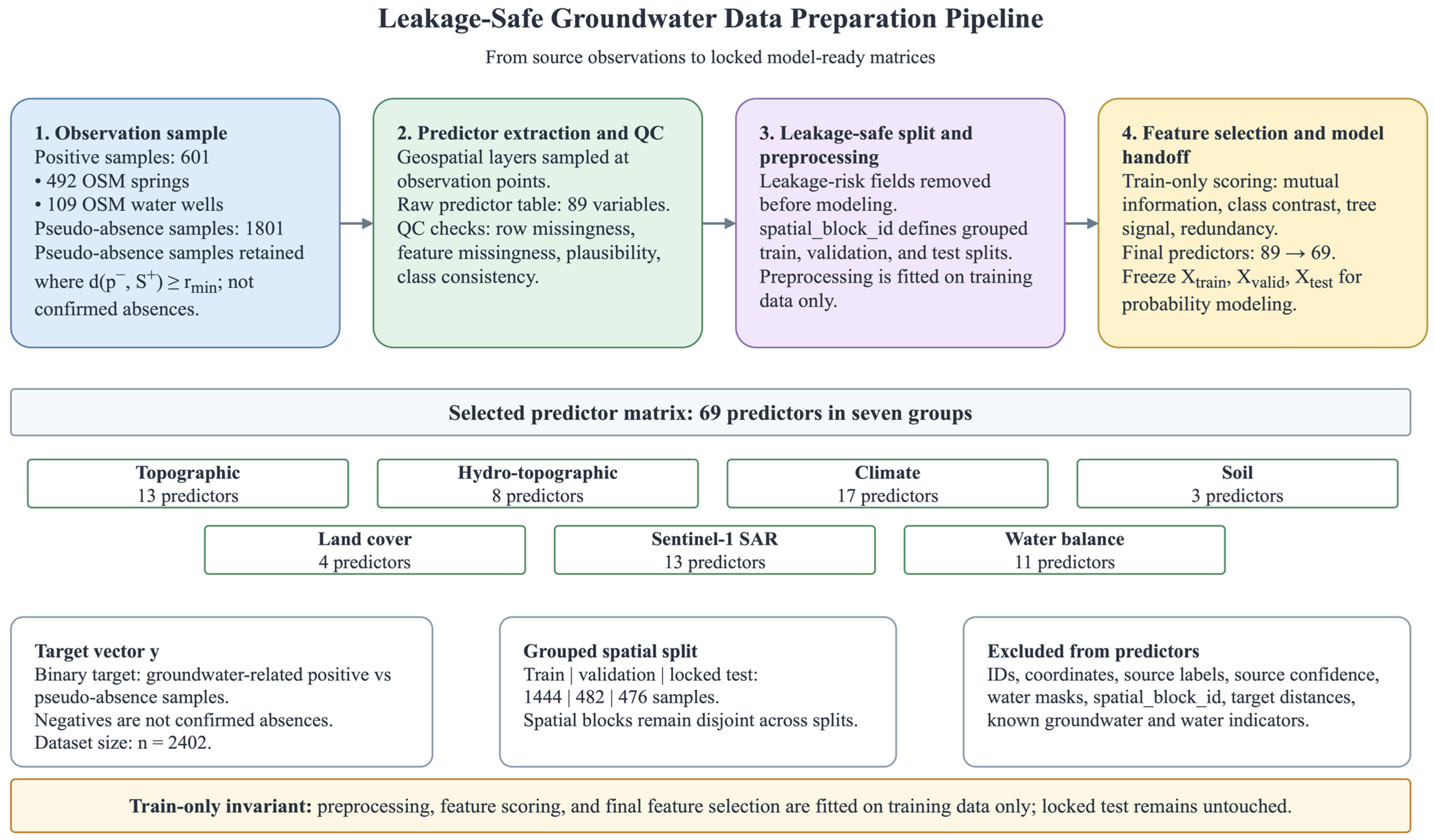
Figure 1 shows the sequential data preparation process prior to model training. The left side of the figure shows the composition of the final analytical sample: the objects of analysis are spatial points $p_i=\left({\lambda }_i,{\phi }_i\right)$, for which a binary target variable $y_i$ and a vector of predictors ${\mathrm{x}}_i$ are formed. 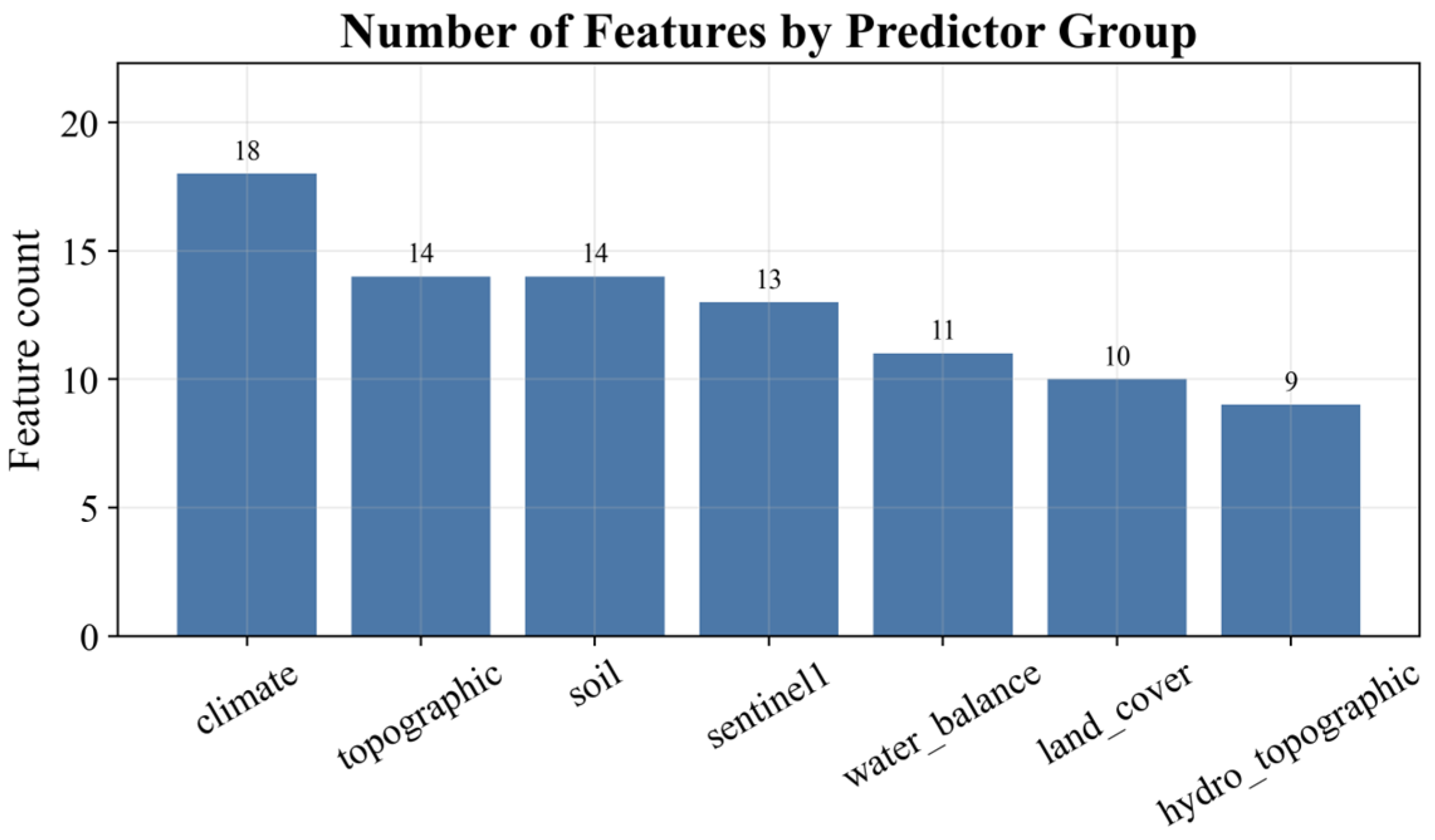After quality control and feature selection, the final matrix ${\mathrm{X}}_{sel}$ includes 69 predictors grouped into seven substantive blocks: topographic, hydrotopographic, climatic, soil, land-cover, Sentinel-1 SAR, and water-balance features. This structure reflects a physically interpretable description of the territory, rather than an arbitrary set of statistical variables. The right side of the figure shows the procedure for forming the leakage-safe sample. First, positive groundwater-related observations and filtered pseudo-absence samples are combined, after which the pseudo-absence points are spatially filtered relative to positive objects. Next, values from the actual geospatial layers are extracted for each point, forming an initial 2402 × 89 feature matrix. The following steps include gap checking, class consistency checking, and the exclusion of variables with the risk of information leakage: coordinates, identifiers, spatial block IDs, distances to target objects, and known groundwater/water indicators.

Data preprocessing to prevent leakage was conducted according to an established protocol. Before model development, metadata fields and all variables directly or indirectly related to the target object were excluded. These included unique identifiers, geographic coordinates, source labels, source credibility attributes, spatial block identifiers, water masks, direct groundwater measurements, and distance-to-target variables. Specifically, variables such as water table, groundwater depth, depth to water, well yield, discharge, pumping rate, NDWI, MNDWI, AWEI, JRC water occurrence frequency, JRC water seasonality, surface water mask, distance to source, distance to well, distance to known groundwater point, and existing groundwater potential maps were excluded from model training to prevent information leakage.

Rows containing more than 30% missing values were removed during quality control. After preprocessing, the dataset contained 2402 observations described by 89 environmental predictors. Feature selection was performed exclusively on the training set using a “training only” protocol. Pairwise correlations were assessed, highly redundant predictors exceeding a predetermined correlation threshold were removed, and the remaining variables were ranked according to their predictive contribution. The final feature set consisted of 69 predictors used in all subsequent experiments. All experiments were conducted using a fixed random number generator seed (42) to ensure reproducibility.

The key methodological element of the scheme is a spatial-block grouped split, in which the data is divided into train, validation, and test parts by spatial blocks, rather than randomly by rows. This reduces the risk of overestimating quality due to spatial autocorrelation. All preprocessing operations, information content assessment, and final feature selection are performed only on ${\mathcal{D}}_{train}$, while validation and locked test are not used to adjust the feature space. Therefore, the final matrix ${\mathrm{X}}_{sel}$ is passed to the modeling as a pre-cleaned, spatially controlled, and leakage-proof basis for estimating the probability $P\left(y_i=l\mid {\mathrm{x}}_i\right)$.

Careful preparation of spatial observations is important because errors introduced during sampling or data pre-processing can significantly affect the reliability of groundwater potential predictions. The sequence of steps ensures traceability of the origin of each observation and each feature: from point generation and extraction of source-sampled layers to the final predictor matrix. This is necessary because, in groundwater-related occurrence suitability mapping, an error during sample preparation can lead to a greater distortion of the results than the choice of a specific classification algorithm. Excluding audit-only fields does not reduce the environmental information available to the model; instead, it prevents technical or spatial identifiers from influencing prediction. Such fields retain their value for quality assurance, data description, and reproducibility. However, these fields should not be used for model training because they may introduce spatially dependent or target-related information. Therefore, the final scheme establishes a strict boundary between the data used to document the sample and the features acceptable for prediction. This makes subsequent model comparison methods consistent and reduces the risk of overinterpreting the obtained metrics.

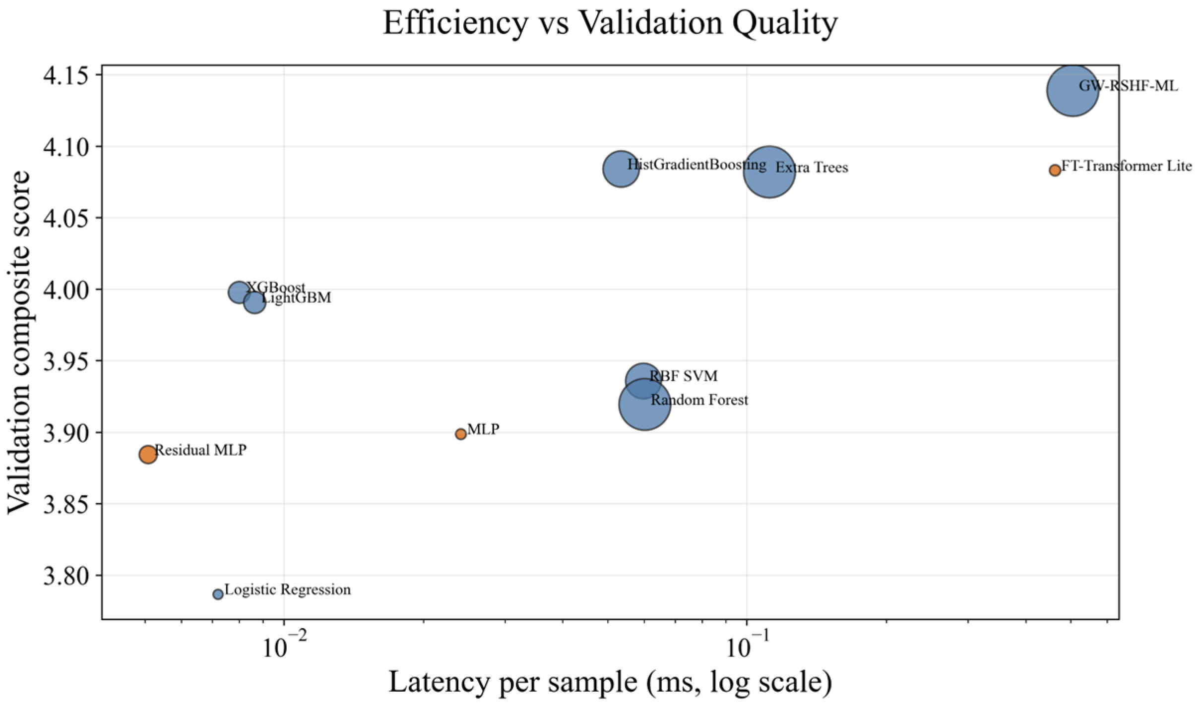
To further evaluate the robustness of the proposed branch selection strategy, an additional stability analysis of repeated spatial partitions was conducted using ten independent spatial partitions. The resulting branch selection frequencies, merge weights, and performance variability are presented in Supplementary Table S1 and Figure S1, demonstrating that the HistGradientBoosting branch remained consistently active across all repeated partitions, while modality-specific branches contributed with varying frequencies depending on the spatial partition. These additional experiments further confirm the robustness of the proposed validation-guided fusion strategy.

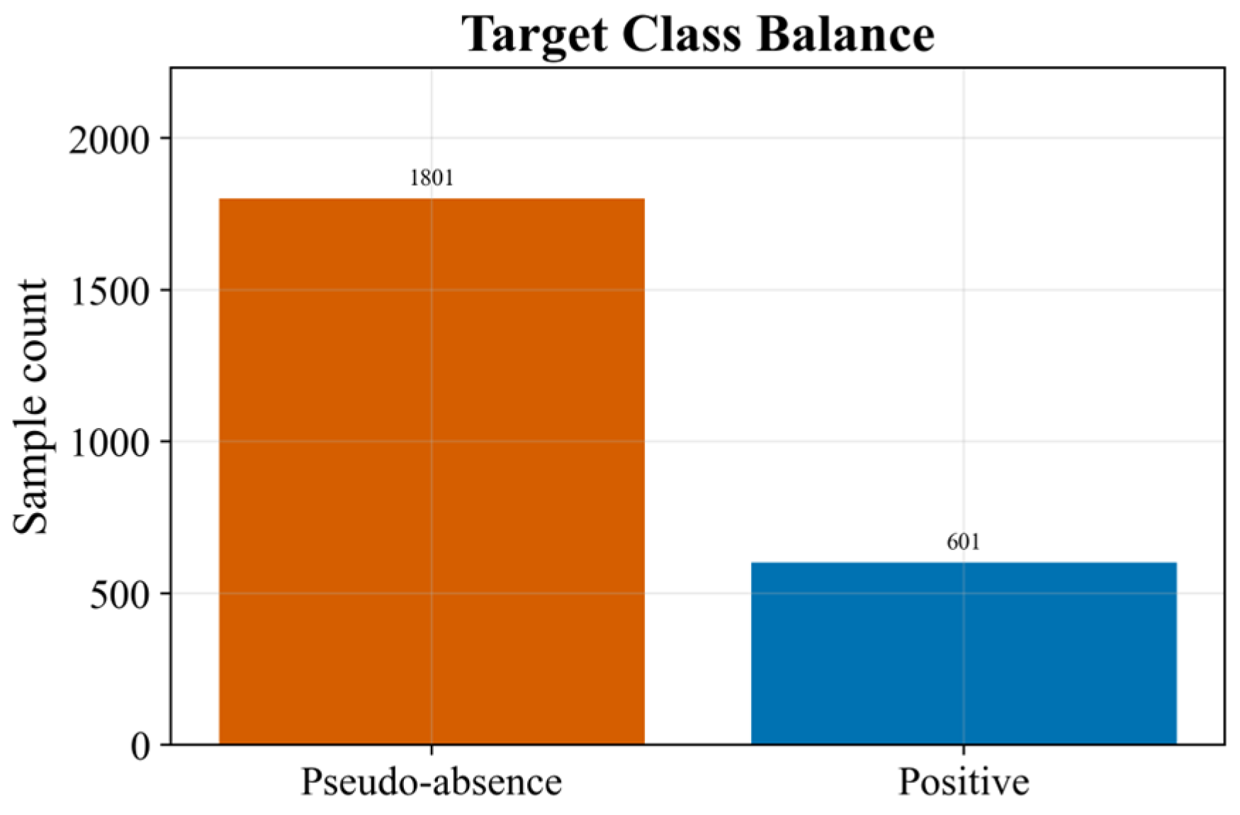
Figure 2 shows the class balance in the final dataset, formed after constructing positive groundwater-related observations and spatially filtered pseudo-absence points. The sample contains 2402 observations: 601 points belong to the positive class and 1801 to the pseudo-absence class. Thus, the ratio of negative to positive classes is approximately 3:1.

This distribution reflects the problem’s deliberate design rather than a data preparation error. The positive class is limited to publicly available observations associated with groundwater occurrences or objects, while pseudo-absence points were generated in greater numbers to form a contrasting spatial background. The pseudo-absence class is not interpreted as a confirmed absence of groundwater; rather, it serves as a comparative category for training the probabilistic model. The presence of moderate class imbalance was taken into account in further analysis of the model quality. Therefore, for evaluation, not only accuracy but also more informative metrics for imbalanced data were used: PR-AUC, F1-score, balanced accuracy, and MCC. This avoids overinterpretation of results due to the dominant class and more accurately assesses the model’s ability to identify groundwater-related conditions.

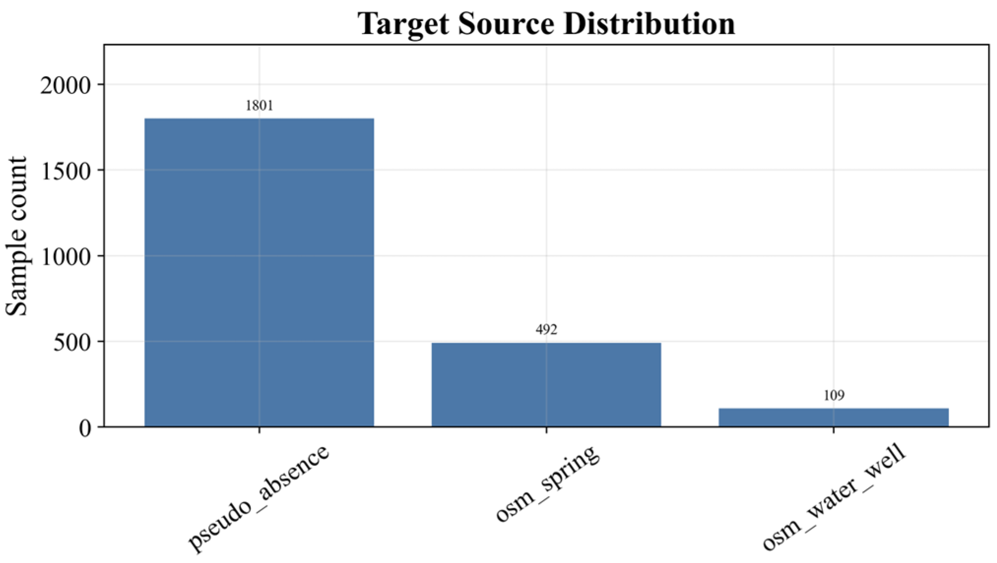
Figure 3 shows the original structure of the observations used to form the target variable. The final sample includes three source categories: pseudo_absence, osm_spring, and osm_water_well. The largest portion consists of 1801 spatially filtered pseudo-absence points, which were used as a contrasting background for binary modeling. The positive class comprises 492 osm_spring and 109 osm_water_well objects, for a total of 601 groundwater-related observations.

This distribution demonstrates that the positive class is not homogeneous in origin: it combines two types of open groundwater-related features, springs and water wells. This enhances the substantive validity of the class, as it reflects not a single specific data source, but several categories of features associated with groundwater occurrence or use. At the same time, the figure highlights an important methodological limitation: the number of osm_water_well features is significantly smaller than that of osm_spring features, so the model should not be interpreted as a specialized well-finding model. In this study, both feature types are used to assess groundwater potential. The pseudo_absence category is considered only as a filtered comparison class and does not indicate the confirmed absence of groundwater.

The study was conducted across Kazakhstan, extending from approximately 40.0° N to 56.8° N and from 45.0° E to 88.5° E, covering an area of approximately 2.72 million km². Kazakhstan is characterized by significant environmental heterogeneity, including vast plains, deserts, semi-deserts, steppes, foothills, and mountainous regions. Climatic conditions range from arid and semi-arid regions in the south and west to more humid continental conditions in the north and northeast, resulting in pronounced spatial variability in precipitation, temperature, evaporation, and water availability. From a hydrogeological perspective, groundwater is located in a variety of aquifer systems, including unconsolidated alluvial deposits, sedimentary basins, fractured bedrock, and mountain aquifers. Groundwater is an important source of drinking water, irrigation water, and industrial water supplies, especially in regions where surface water resources are limited or highly seasonal. The high environmental diversity and uneven spatial distribution of groundwater observations make Kazakhstan a suitable testing ground for spatially aware machine learning methods using multimodal geospatial predictors.

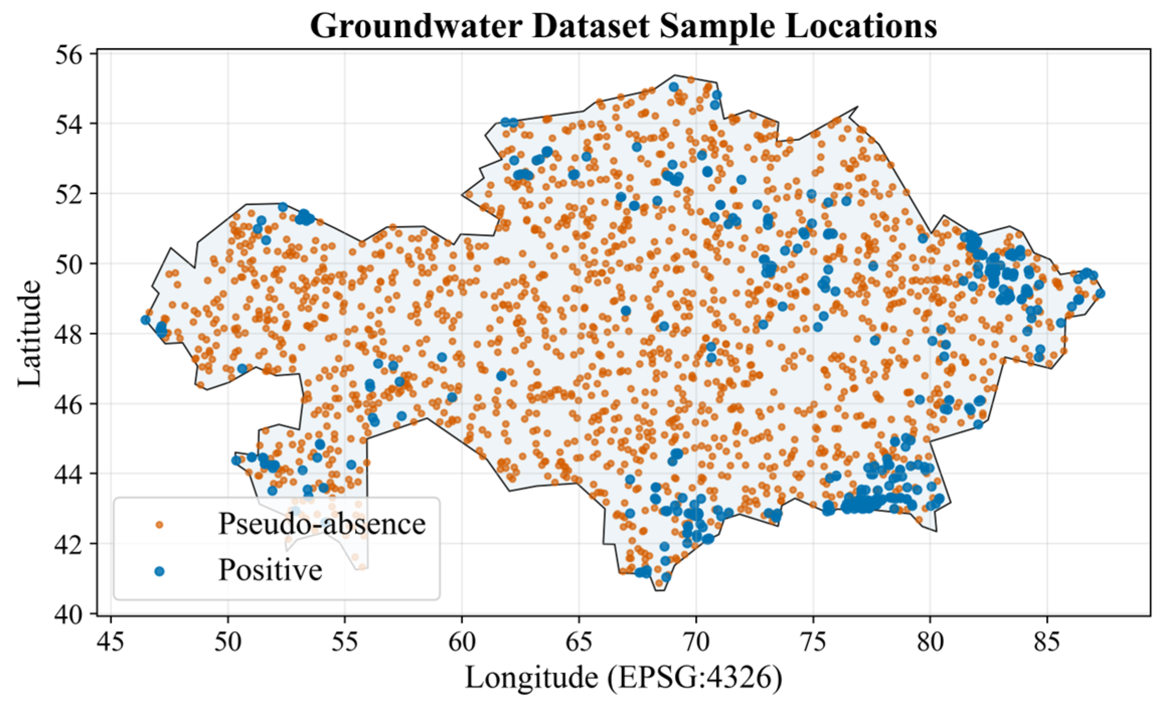
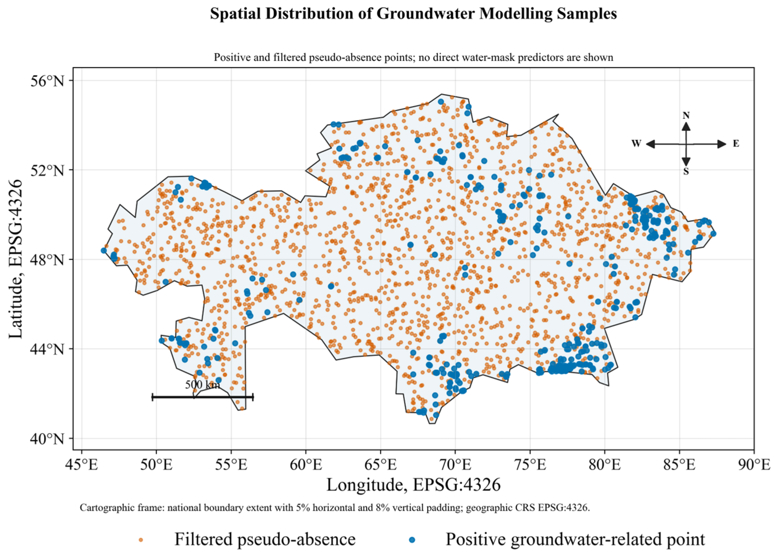
Figure 4 shows the geographic distribution of the final dataset points in the EPSG:4326 coordinate system. The contour delimits the study area, within which two types of observations are located: positive groundwater-related points and spatially filtered pseudo-absence points. This presentation allows visual verification that the sample covers the main analysis area and is not concentrated in isolated regions. Pseudo-absence points are distributed throughout the study area and form the spatial background necessary for comparison with positive observations. Positive points exhibit more pronounced clustering, which is expected for open data on springs and water wells: such objects are typically recorded unevenly and depend on both natural conditions and the availability of observations. Therefore, the spatial heterogeneity of the positive class was taken into account in subsequent stages through spatial block partitioning.

The figure also confirms that the analysis was performed on real coordinate objects, not on an abstract tabular sample. However, the coordinates themselves were used to construct the sample, control the spatial structure, and visualize it, but were not included in the final set of predictors. This reduces the risk of spatial leakage and ensures that subsequent modeling is focused on the natural features of the area, rather than on the direct memorization of point locations.

The proposed framework is based on multimodal geospatial datasets representing topographic, climate, hydrological, soil, land-use, and radar information. Because these datasets were obtained from different providers and have different spatial and temporal characteristics, they were harmonized prior to feature extraction.

Table 2. Characteristics of geospatial datasets used for assessing groundwater environmental suitability.

Data Group	Source	Period	Resolution	Preprocessing	Missing-Value Handling	License	Purpose
Positive observations	OpenStreetMap	2025	Point	Duplicate removal, AOI filtering	Not applicable	ODbL	Target labels
DEM	NASA SRTM	Static	30 m	Terrain derivatives	No missing values	Public	Topography
Climate	TerraClimate	2018–2025	~4 km	Seasonal aggregation	Train-only imputation	Public	Climate
Sentinel-1 SAR	Copernicus	2018–2025	10 m	Seasonal composites	Train-only imputation	Copernicus	Surface moisture
Land Cover	ESA WorldCover	2021	10 m	Fraction calculation	No missing values	ESA	Land cover
Soil	OpenLandMap	Static	250 m	Resampling	Train-only imputation	OpenLandMap	Soil
Water balance	MOD16A2GF/TerraClimate	2018–2025	500–4000 m	Annual aggregation	Train-only imputation	Public	Water balance

provides a summary of the geospatial datasets used in this study, including their source, temporal coverage, spatial resolution, preprocessing procedure, missing value handling, license, and role in the proposed framework.

All raster data were resampled to a common working resolution of 250 m before feature extraction. Predictor values were extracted only at observation sites, resulting in a feature table with point sampling. Missing values were estimated separately for each predictor and imputed exclusively using statistics obtained from the training set to prevent information leakage. All spatial datasets were processed in the EPSG:4326 coordinate system.

2.3. Study of Distributions and Information Content of Feature Space

Table 3. Descriptive statistics of the first thirty geospatial predictors of the final dataset.

Feature	Count	Mean	Std	Min	25%	50%	75%	Max
elevation	2402	525.2465	679.4197	−68.0000	136.0000	312.0000	578.7500	4199.0000
slope	2402	2.6137	5.4458	0.0000	0.0000	1.0000	2.0000	46.0000
aspect_sin	2402	−0.0023	0.6889	−1.0000	−0.7040	0.0000	0.7040	1.0000
aspect_cos	2402	0.1238	0.7145	−1.0000	−0.5592	0.2079	0.8192	1.0000
hillshade	2402	180.0808	13.0431	81.0000	179.0000	180.0000	181.0000	255.0000
local_relief	2402	20.0262	41.3947	0.0000	2.0000	4.0000	14.0000	495.0000
tpi_250 m	2402	−1.0299	5.9205	−53.6000	−0.8000	−0.2000	0.4000	57.2000
tpi_1000 m	2402	−4.7933	23.8316	−215.3673	−2.5918	−0.4286	0.7347	155.9600
roughness	2402	20.0262	41.3947	0.0000	2.0000	4.0000	14.0000	495.0000
curvature_proxy	2402	14.2211	77.7872	−717.0000	−5.0000	2.0000	10.0000	774.0000
tpi_500 m	2402	−2.2105	11.5211	−95.6923	−1.3846	−0.2308	0.5385	99.3080
tpi_2000 m	2402	−7.4032	42.8756	−359.1117	−4.2411	−0.5051	1.1269	270.4100
slope_relief_interaction	2402	11.0631	27.7546	0.0000	0.0000	1.6094	5.4161	283.8000
terrain_dissection_index	2402	0.0457	0.0639	0.0000	0.0122	0.0251	0.0548	1.3067
flow_accumulation	2401	1206.7005	27,307.0018	1.0000	1.0000	2.0000	7.0000	1,038,300.0000
log_flow_accumulation	2401	1.7688	1.7118	0.6931	0.6931	1.0986	2.0794	13.8530
upstream_drainage_area	2402	50.7944	1587.4782	0.0049	0.0101	0.0265	0.1430	75,491.0000
hand	2402	17.6331	46.2881	0.0000	1.0250	3.1750	12.1438	603.3800
valley_bottom_proxy	2402	0.9002	0.2041	0.0000	0.9190	0.9788	0.9932	1.0000
drainage_tendency_index	2401	1.1067	1.4044	0.0144	0.3466	0.6931	1.1989	13.8530
topographic_wetness_index_proxy	2401	1.0385	1.8964	−3.1781	0.0000	0.6931	1.3863	13.8530
stream_power_index_proxy	2401	0.0915	0.2812	0.0000	0.0000	0.0121	0.0547	4.0922
relative_valley_position	2402	0.9199	0.1782	0.0000	0.9393	0.9841	0.9949	1.0000
annual_precipitation_mean	2402	251.2775	118.2260	69.7500	150.6562	246.2500	303.6562	699.3800
wet_season_precipitation	2402	90.7747	48.8370	28.1250	55.1250	78.1875	106.5000	302.3800
dry_season_precipitation	2402	61.0790	47.6766	2.5000	21.8750	47.6875	92.2500	222.7500
precipitation_seasonality	2402	0.1398	0.1539	−0.1359	0.0093	0.1046	0.2628	0.4670
precipitation_cv	2402	0.2211	0.0563	0.0874	0.1808	0.2119	0.2576	0.4190
mean_air_temperature	2402	7.0129	4.2378	−8.9036	3.9650	6.9467	10.4863	15.9980
warm_season_temperature	2402	19.9947	4.4383	1.1667	17.3738	20.5976	23.3571	27.8760

presents descriptive statistics for the first thirty features used in the initial analysis of the data structure. These variables belong to three key groups of factors: topography, hydrotopography, and climate. For each feature, the number of available observations, mean, standard deviation, minimum, quartile values, and maximum are shown. This table was used to control ranges, identify missing values, assess feature dispersion, and check the physical plausibility of values prior to model training.

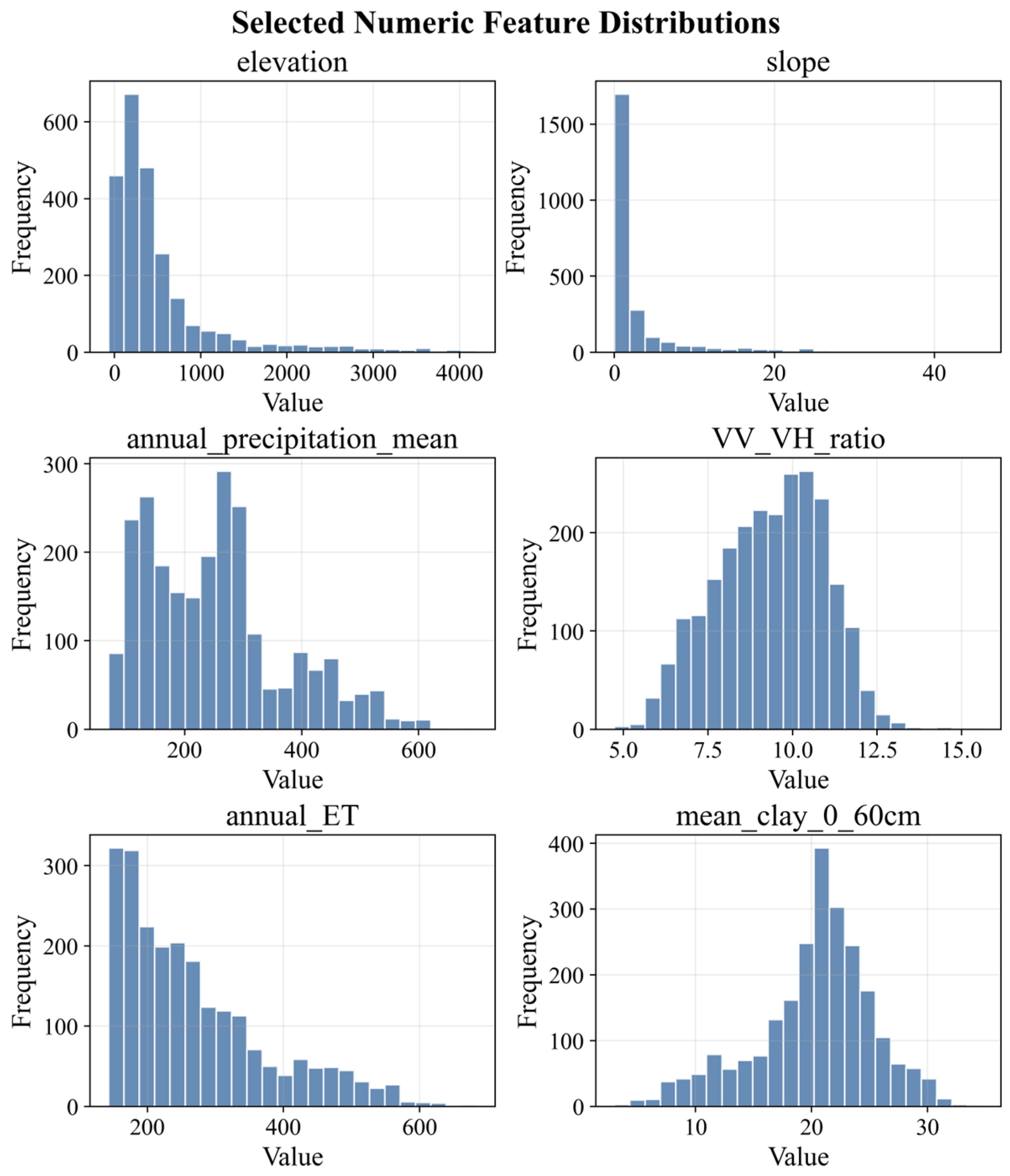
Therefore, this table represents a fragment of the overall feature statistics, not a complete list of all variables in the dataset. The full original feature space contained 89 features, and after train-only selection, 69 features were used for modeling. Figure 5 shows the distribution histograms of six numerical features selected for the initial validation of the data structure: elevation, slope, annual_precipitation_mean, VV_VH_ratio, annual_ET, and mean_clay_0_60 cm. These variables reflect different groups of factors—topography, climate, radar response, water balance, and soil characteristics so their joint analysis allows us to assess the heterogeneity of the feature space before model training.

The elevation and slope distributions exhibit a pronounced right-hand asymmetry: most observations are located in relatively low-lying, gently sloping areas. At the same time, isolated high-altitude and steeper areas are also present. A similar asymmetry is observed for annual_ET, indicating heterogeneity in evaporation conditions and water balance. The annual_precipitation_mean feature exhibits a multimodal distribution, reflecting the territory’s climatic heterogeneity and differences between drier and wetter zones. The VV_VH_ratio distribution appears more compact and closer to unimodal, indicating a relatively stable range of Sentinel-1 radar ratios in the sample. The soil indicator mean_clay_0_60 cm also shows a pronounced central range but retains sufficient variability to describe soil water-retention properties. Taken together, the figure confirms that the features have different scales, distribution shapes, and degrees of skewness, so supervised preprocessing procedures were required before modeling, including handling missing values, scaling, and selecting informative variables for training. 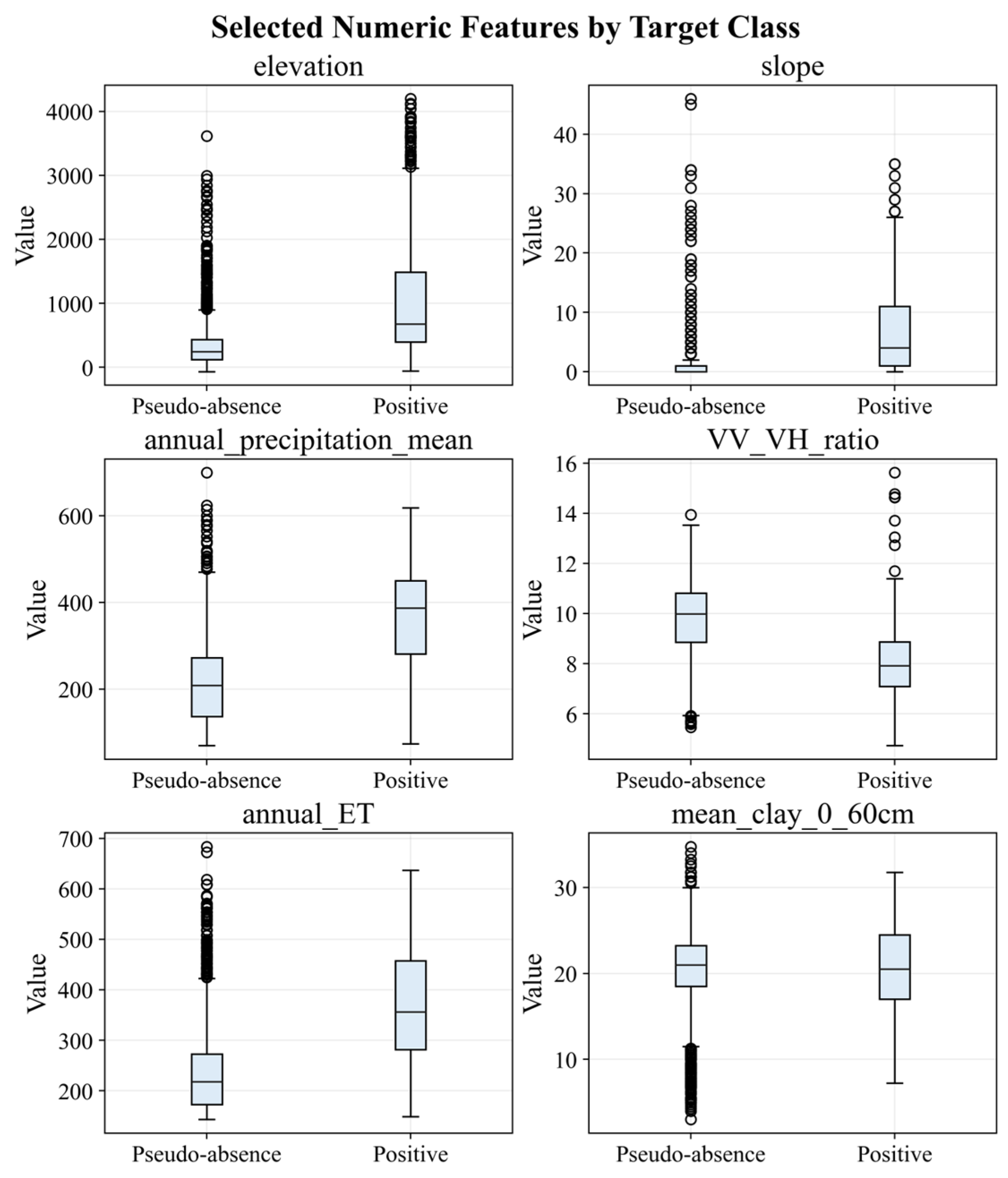Figure 6 presents boxplots of six numerical features for the Pseudo-Absence and Positive classes. This visualization was used for an initial assessment of whether conditions at groundwater-related observation points differ from those of the spatially filtered background class before model training.

The elevation, slope, annual_precipitation_mean, and annual_ET features show that the positive class is, on average, biased toward higher values. This indicates that known groundwater-related points are more often associated with areas where topography, climatic moisture, and water balance differ from the conditions observed in most pseudo-absence locations. Differences are particularly noticeable for precipitation and evapotranspiration: the medians of the positive class are higher, and the interquartile ranges show a more pronounced concentration in relatively moist conditions. For VV_VH_ratio, the opposite pattern is observed: the positive class has a lower median compared to pseudo-absence. This may reflect differences in the surface radar response associated with cover type, landscape structure, or moisture conditions. The soil indicator mean_clay_0_60 cm shows partial overlap between classes but retains differences in ranges and outliers, indicating its potential additional information content. The presence of outliers in both classes was not considered an error in itself, as geospatial features naturally exhibit high spatial heterogeneity. The figure confirms that the selected variables contain a discriminatory signal between classes, but no single feature alone provides complete separation. Therefore, further modeling was based on a multi-feature approach, in which the final probability is derived from the combined use of topographic, climatic, SAR, soil, and water-balance factors. 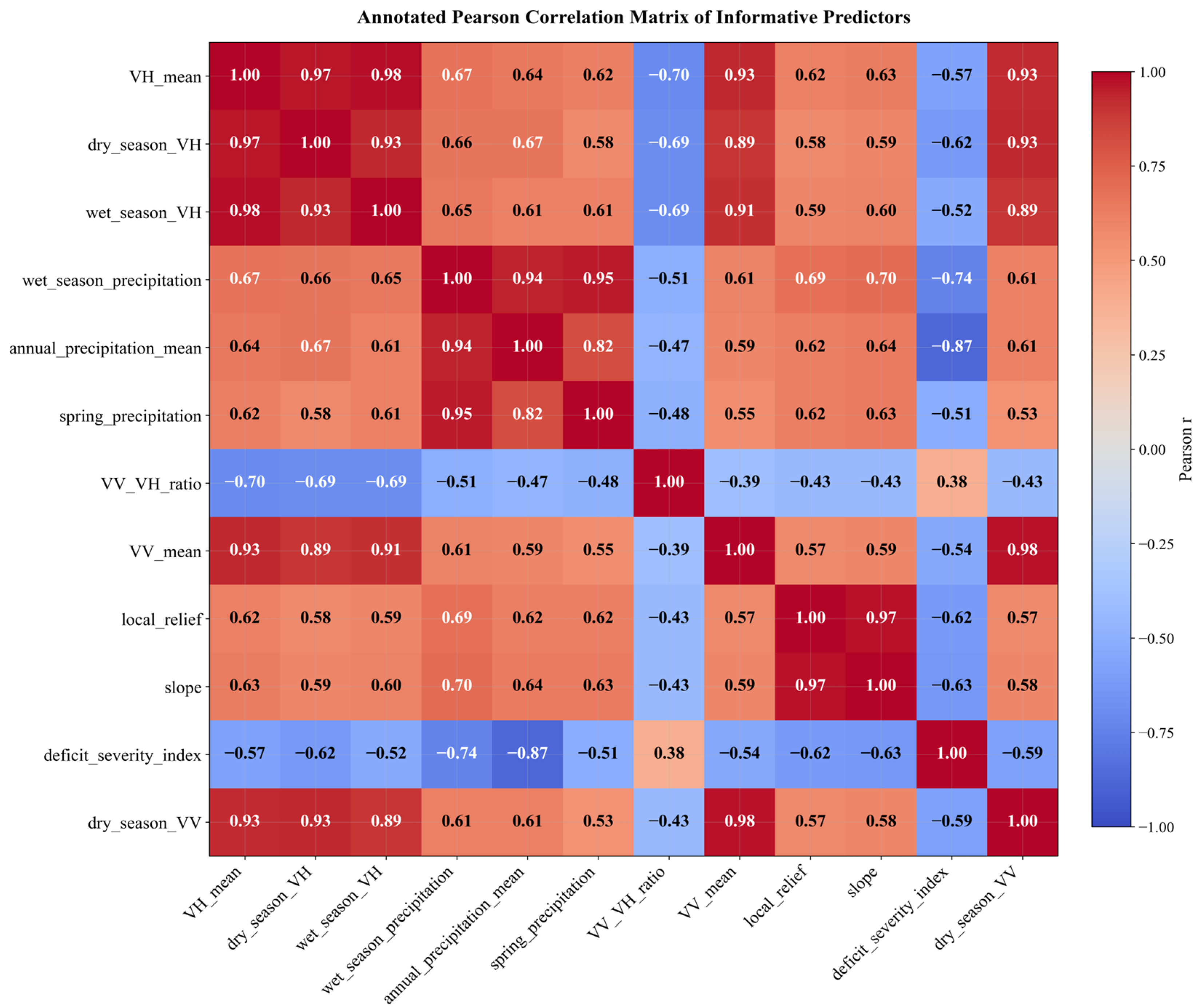Figure 7 shows the annotated Pearson correlation matrix for the group of most informative features identified during the preliminary analysis.

The matrix was used to assess linear relationships among variables and to identify potential redundancies in the feature space before final predictor selection. The most pronounced positive correlations are observed within homogeneous groups of features. The Sentinel-1 SAR metrics VH_mean, dry_season_VH, wet_season_VH, VV_mean, and dry_season_VV are strongly correlated, reflecting the similar nature of radar seasonal characteristics. Similarly, the climate metrics wet_season_precipitation, annual_precipitation_mean, and spring_precipitation exhibit high positive correlations, as they describe related components of the precipitation regime. The topographic metrics local_relief and slope are also highly correlated, as expected for areas with pronounced relief discontinuities.

Negative correlations are particularly evident for deficit_severity_index, which shows inverse relationships with precipitation variables and several SAR/terrain metrics. This is logical, as increasing climate deficits are typically contrasted with higher moisture conditions. The VV_VH_ratio feature also shows negative correlations with most SAR indices and moderate inverse correlations with climate variables, indicating its independent role relative to absolute VV/VH values. Thus, the figure confirms the presence of both informative relationships and partial multicollinearity between the predictors. Therefore, subsequent train-only feature selection was necessary to preserve the useful signal while simultaneously removing weak or redundant variables.

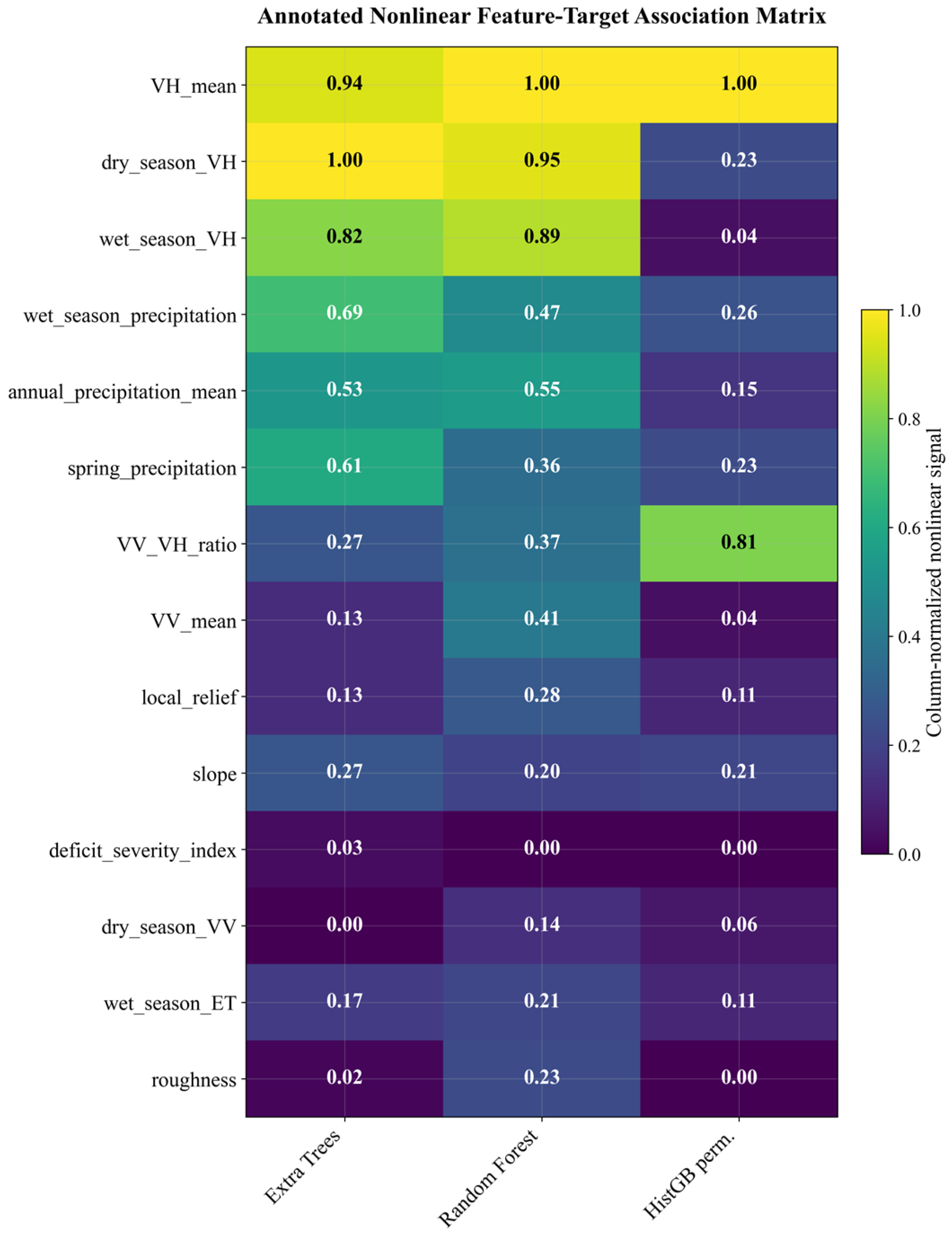
Figure 8 shows the annotated matrix of normalized nonlinear signal relationships between the selected features and the target variable. The evaluation was performed using three tree-based approaches: Extra Trees, Random Forest, and permutation-based evaluation for HistGradientBoosting. The cell values are normalized from 0 to 1 within each column, so the figure reflects the relative importance of the features within the respective method rather than the absolute magnitude of the effect. The most consistent signal is observed for the SAR features VH_mean, dry_season_VH, and wet_season_VH. These variables rank among the top in several models, indicating their strong ability to distinguish between positive groundwater-related points and pseudo-absence observations in the multi-feature space. Climate indicators, especially wet_season_precipitation, annual_precipitation_mean, and spring_precipitation, also demonstrate a significant relationship with the target class, consistent with the hydrological role of the moisture regime. The VV_VH_ratio feature shows a particularly high signal in the HistGradientBoosting permutation estimate, indicating its independent informativeness when accounting for nonlinear interactions.

In contrast, deficit_severity_index, dry_season_VV, and roughness have low values in most columns, so their individual contribution to the feature group under consideration is limited. Thus, the figure confirms that a single factor does not drive the strongest relationship with the target variable; rather, a combination of SAR, climatic, and individual topographic features does. The results show that groundwater-related observations are influenced by multiple interacting environmental factors rather than any single factor, highlighting the importance of integrating climate, elevation, radar and soil information to assess regional groundwater potential.

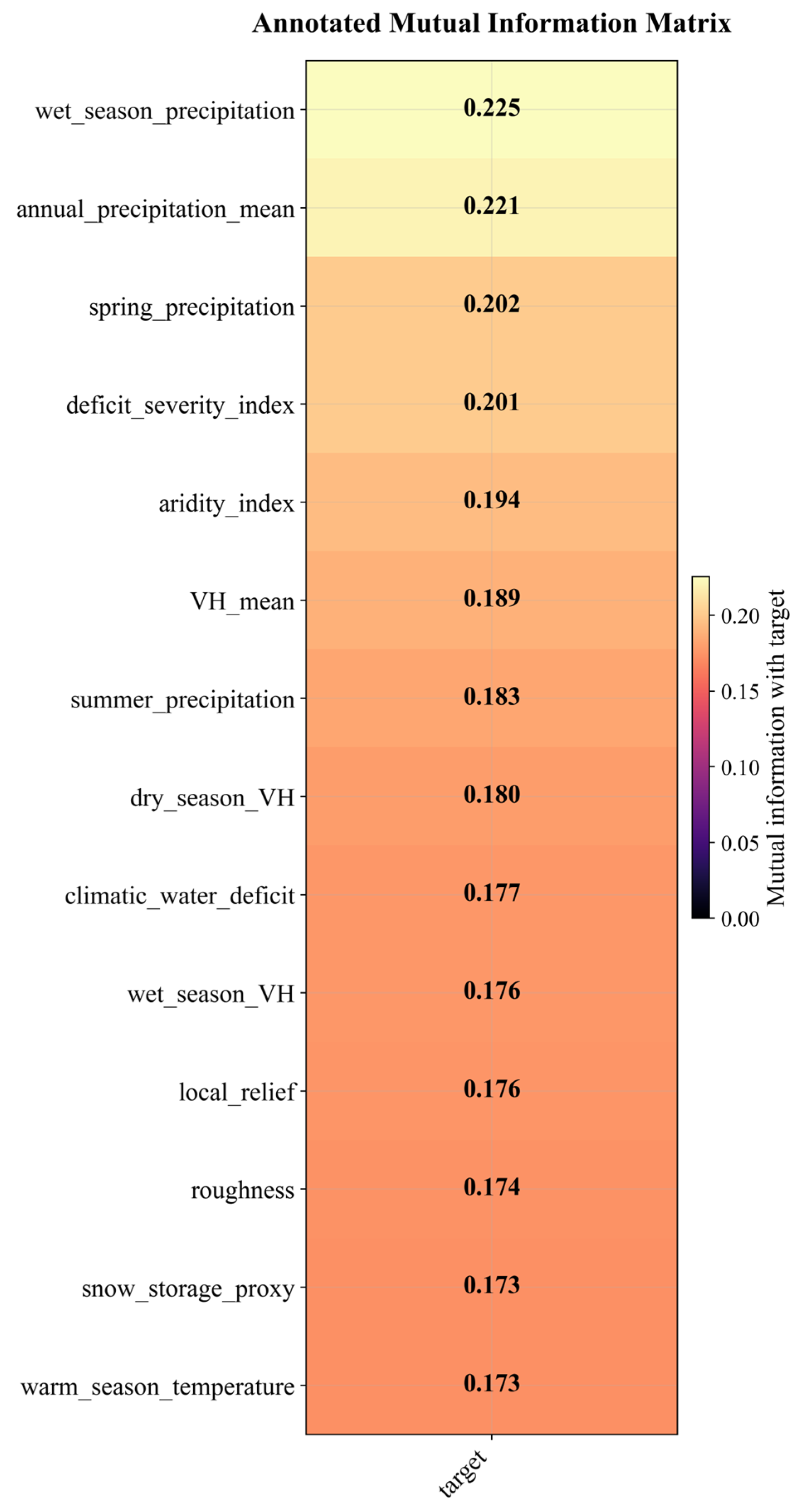
Figure 9 shows the annotated mutual information matrix for the group of features that demonstrated the strongest relationship with the target variable. Unlike correlation analysis, mutual information was used to identify not only linear but also more complex nonlinear relationships between individual predictors and the target class. The values in the figure reflect the information contribution of each feature to distinguish between positive groundwater-related points and pseudo-absence observations.

The highest mutual information values were obtained for the climatic features wet_season_precipitation (0.225), annual_precipitation_mean (0.221), and spring_precipitation (0.202). This demonstrates that the moisture regime and seasonal precipitation distribution contain the most pronounced individual signal relative to the target class. High values are also observed for deficit_severity_index (0.201) and aridity_index (0.194), which further confirms the importance of climatic water deficit and aridity in assessing groundwater potential.

Among the radar features, VH_mean (0.189), dry_season_VH (0.180), and wet_season_VH (0.176) have a significant contribution, indicating the informativeness of Sentinel-1 SAR indicators as a supplement to climatic factors. The topographic features local_relief (0.176) and roughness (0.174) demonstrate a moderate but stable relationship with the target variable. The features snow_storage_proxy and warm_season_temperature, with values of 0.173, are also included in the group of informative factors, although their contribution is lower than that of the leading precipitation-related variables. Thus, the figure demonstrates that the strongest individual signal is formed primarily by climatic and water-balance characteristics, while SAR and terrain indicators play a supporting but substantively important role. These results were used as part of a train-only analysis of feature informativeness and confirmed the feasibility of subsequent multi-feature modeling.

3. Results

3.1. Machine Learning Models and Probabilistic Modeling Framework

After forming the leakage-safe feature matrix ${\mathrm{X}}_{sel}\in {ℝ}^{2402\times 69}$, the problem was reduced to binary probabilistic classification. For each observation i, the model $M_m$ obtains the selected feature vector ${\mathbf{x}}_i^{*}\in {ℝ}^{69}$ and returns the probability of belonging to the positive groundwater-related class (31):

$${\widehat{p}}_i^{\left(m\right)}=f_m\left({\mathrm{x}}_i^{*}\right),{\widehat{p}}_i^{\left(m\right)}=P_m\left(y_i=1\mid {\mathrm{x}}_i^{*}\right)$$

(31)

All models were trained on ${\mathcal{D}}_{train}$, classification thresholds and best configuration selection were performed on ${\mathcal{D}}_{valid}$, and ${\mathcal{D}}_{test}$ was saved as a locked test split for final validation. This arrangement eliminates the use of test labels when selecting features, setting thresholds, and comparing architectures. Regularized logistic regression (32) was used for the linear baseline model:

$${\widehat{p}}_i^{\left(LR\right)}=\sigma \left({\beta }_0+{\displaystyle {{\displaystyle \sum }}_{k=1}^{69}}{\beta }_k{x}_{ik}^{*}\right),\sigma \left(z\right)={\displaystyle \frac{1}{1+\exp \left(-z\right)}}$$

(32)

Tree-based models generated the probability as an aggregated result of an ensemble of trees (33):

$${\widehat{p}}_i^{\left(ens\right)}={\displaystyle \frac{1}{T}}{\displaystyle {{\displaystyle \sum }}_{t=1}^T}{h}_t\left({\mathrm{x}}_i^{*}\right)$$

(33)

where $h_t\left(\cdot \right)$ is an individual tree or the base predictor of the ensemble, and $T$ is the number of trees. For boosting models, the probability was constructed as a sequential sum of weak models (34):

$${\widehat{p}}_i^{\left(boost\right)}=\sigma \left({\displaystyle {{\displaystyle \sum }}_{t=1}^T}{\eta }_t{h}_t\left({\mathrm{x}}_i^{*}\right)\right)$$

(34)

For RBF SVM, the separating function was first estimated in the nonlinear kernel space, after which the probabilities were obtained via calibrated probabilistic inference (35):

$${\widehat{p}}_i^{\left(SVM\right)}=\sigma \left(A g\left({\mathbf{x}}_i^{*}\right)+B\right)$$

(35)

The neural network models were trained on a pre-processed feature matrix, where, after one-hot encoding, the input dimension was 78. The general form of the DL models is written as (36):

$${\widehat{p}}_i^{\left(DL\right)}=\sigma \left(g_{\theta }\left({\mathbf{z}}_i\right)\right)$$

(36)

where ${\mathbf{z}}_i$ is the preprocessed input vector, g_θ is the neural network function, and $\theta$ are the trainable parameters. Training was performed with weighted binary cross-entropy, the AdamW optimizer, and early stopping using PR-AUC validation. The aggregated validation metric (37) was used to compare the models:

$$S_{valid}=PR\text{-}AUC+ROC\text{-}AUC+F1+BA+MCC-Brier$$

(37)

The binary decision was formed using the validation-selected threshold (38):

$${\widehat{y}}_i^{\left(m\right)}=\mathbb{1}\left[{\widehat{p}}_i^{\left(m\right)}\ge {\tau }_m\right]$$

(38)

Table 4. Descriptive statistics of the main features of the final data set.

Model	Family	Main Hyperparameters	Role in the Experiment	Methodological Explanation
Logistic Regression	Linear ML	solver = liblinear, C = 1.0, max_iter = 2000, class_weight = balanced	Simple linear baseline model	Checks whether linear separation is sufficient in a 69-dimensional space
Random Forest	Bagging/tree ensemble	n_estimators = 240, min_samples_leaf = 2, class_weight = balanced	Nonlinear robust baseline	Used to test nonlinear patterns without boosting
Extra Trees	Randomized tree ensemble	n_estimators = 300, min_samples_leaf = 2, class_weight = balanced	Strong tree-based baseline	Evaluates the contribution of strongly randomized trees and feature interactions
HistGradientBoosting	Gradient boosting	max_iter = 160, learning_rate = 0.045, l2_regularization = 0.08, max_leaf_nodes = 15	One of the strongest classical ML baselines	Checks the quality of regularized boosting on tabular geospatial data
RBF SVM	Kernel ML	C = 1.5, gamma = scale, probability = True, class_weight = balanced	Margin-based baseline	Used to test nonlinear separation via an RBF kernel
XGBoost	Gradient boosting	n_estimators = 160, max_depth = 2, learning_rate = 0.045, subsample = 0.9, colsample_bytree = 0.9	Boosting baseline	Limited tree depth reduces the risk of overfitting on a small sample
LightGBM	Gradient boosting	n_estimators = 160, learning_rate = 0.045, num_leaves = 7, min_child_samples = 5, class_weight = balanced	Alternative boosting baseline	Checks the robustness of the result to another boosting algorithm
MLP	Deep learning	hidden = 64, dropout = 0.20, AdamW, weighted BCE, early stopping	Basic neural network model	Used as a simple DL baseline for tabular features
Residual MLP	Deep learning	width = 64, residual blocks = 2, dropout = 0.15, AdamW	Improved MLP baseline	Checks whether residual representation is helpful for tabular features
FT-Transformer Lite	Deep tabular model	dim = 24, heads = 4, layers = 1, dropout = 0.10	Strong DL baseline	Used to test attention-based feature processing
GW-RSHF-ML	Proposed hybrid ML	11 probability expert branches; validation-selected sparse convex fusion	Proposed model	Combines full-feature and modality-specific branches, but selects weights only based on validation data

presents the machine learning models used for the comparative experiment on probabilistic groundwater-related occurrence suitability mapping. The table lists the model families, key hyperparameters, their role in the experimental design, and methodological purpose. Linear, ensemble, boosting, kernel-based, and neural network models were considered as baseline approaches, enabling us to evaluate the performance of both simple and more complex nonlinear algorithms on a single feature space. The proposed hybrid GW-RSHF-ML model, which combines full-feature and modality-specific probabilistic branches with weight selection only on the validation split, is presented separately. This comparison is necessary for an objective assessment of whether the proposed hybrid approach provides an advantage over classical and modern baseline models.

In the final part of the experiment, the proposed GW-RSHF-ML model was implemented. Its goal was not to replace all baseline models with a single “complex” architecture, but to test whether the hydrological fusion approach can robustly combine different signal types: a common multi-feature signal and signals from individual physically interpretable groups. Each expert branch $b$ receives its own subset of features ${\mathcal{I}}_b$ and generates its own probability (39):

$$p_{ib}=P_b\left(y_i=1\mid {\mathbf{x}}_{i,{\mathcal{I}}_b}^{*}\right)$$

(39)

Within GW-RSHF-ML, full-feature branches and modality-specific branches were used. Full-feature branches worked with all 69 features, while modality-specific branches used individual groups: topographic, hydro-topographic, climate, soil, land-cover, Sentinel-1 SAR, and water-balance predictors. The final merging was performed using sparse convex fusion (40):

$$w_b\ge 0,{\displaystyle {{\displaystyle \sum }}_{b=l}^B}{w}_b=1$$

(40)

For the chosen validation configuration, three branches were active: the full-feature Extra Trees interaction branch, the topographic branch, and the Sentinel-1 SAR branch. Therefore, the resulting probability can be compactly written as (41):

$${\widehat{p}}_i=\alpha p_{i,3}+\beta p_{i,5}+\gamma p_{i,10},\alpha ,\beta ,\gamma \ge 0,\alpha +\beta +\gamma =1$$

(41)

Here, $p_{i,3}$ is the probability of the full-feature nonlinear interaction branch, $p_{i,5}$ is the probability of the topographic modality branch, and $p_{i,10}$ is the probability of the Sentinel-1 SAR branch. In the trained configuration, the weights were not obtained manually, but through validation-guarded selection. Therefore, the correct interpretation of the model is that the contribution of the branches is determined by the data and the validation procedure, and not by expert assignment of coefficients. The final binary decision was formed using the validation-selected threshold (42):

$${\widehat{y}}_i=\mathbb{1}\left[{\widehat{p}}_i-\tau \ge 0\right]$$

(42)

Figure 10 shows the internal structure of GW-RSHF-ML as an ensemble of parallel probabilistic expert branches. The input is a selected 69-dimensional feature vector ${\mathbf{x}}^{*}\in {ℝ}^{69}$, formed after leakage-safe data preparation and train-only feature selection. The architecture is divided into two groups of branches: full-feature expert branches and feature-modality expert branches.

Full-feature branches use the entire feature set and test different types of statistical signal: regularized linear dependence, bagging structure, nonlinear interactions, and margin-based splitting. Modality-specific branches work with individual physically interpretable feature blocks: topographic, hydrotopographic, climate, soil, land cover, Sentinel-1 SAR, and water balance. This principle allows us to test which groups of factors independently contribute to the probability of groundwater potential.

Each branch returns its own probability, $p_b$, after which a branch probability vector is formed. Validation-selected sparse convex fusion is then applied. These results indicate that the model does not mechanically average all branches or manually assign weights. Instead, the procedure selects the combination of branches that yields the most stable result in the validation split. In the final configuration, the nonlinear interaction branch, topographic branch, and Sentinel-1 SAR branch remained active, while the remaining branches received zero coefficients in sparse fusion. The decision layer uses a validation threshold $\tau$, after which a binary forecast $\widehat{y}$ is generated. Notably, the test split does not participate in branch selection, coefficient selection, or threshold selection. Therefore, the scheme reflects not simply an ensemble of models, but a validation-controlled hydrological fusion pipeline designed for probabilistic groundwater-potential modeling without leaking test information.

3.2. Analysis of the Latent and Spatial Structure of Geospatial Data

Figure 11 shows a two-dimensional PCA projection of informative features, where points are colored by true class: Positive and Pseudo-Absence. The first principal component explains 51.0% of the variance, while the second explains 12.2%, accounting for 63.2% of the variation in the selected feature space. This visualization was not used for model training, but rather for diagnostic assessment of the data’s internal structure and the possible separability of classes in reduced dimensions. The distribution of points shows that the classes are not completely linearly separable. In the central region of the projection, there is a significant overlap of positive and pseudo-absence samples. This confirms that the problem cannot be reduced to a simple threshold rule based on a single or a few principal components. Positive observations are also more often shifted to the left and more dispersed part of the space, while pseudo-absence points form a denser cluster in the right part of the projection. This PCA structure indicates the presence of a discriminating multivariate signal but also reveals its nonlinearity and partial ambiguity. Therefore, the continued use of tree-based, DL, and hybrid models was methodologically justified: they can account for complex interactions among climatic, SAR, topographic, and water-balance features. The figure also confirms the need for probabilistic classification, as some observations lie in the overlap zone between classes and should not be interpreted as completely unambiguous.

Figure 12 presents a visualization of the results of unsupervised KMeans_k2 clustering in the space of two principal components constructed using the informative features of the dataset. The first principal component explains 51.0% of the variance, and the second 12.2%. Therefore, this projection reflects the underlying structure of the feature space and allows one to assess the internal heterogeneity of the sample without using the target variable.

Cluster 0 forms a more compact and dense group of observations, concentrated primarily in the right side of the PCA space. Cluster 1, in contrast, is characterized by a wider dispersion and occupies the left side of the projection, encompassing observations with greater variability in their principal components. The boundary between the clusters is quite clearly defined, although partial overlap remains in the transition zone, indicating the absence of a completely rigid separation. This structure demonstrates the existence of natural heterogeneity in the feature space, detectable even without class labels. This is important from an analytical perspective, as it confirms the presence of internal subgroups of observations associated with differences in combinations of topographic, climatic, SAR, and water balance characteristics. However, clusters should not be interpreted as a direct replacement for the Positive and Pseudo-Absence target classes: the KMeans algorithm minimizes intracluster variance rather than solving the problem of classification based on groundwater-related labels. Thus, the figure confirms that the sample has its own latent structure, and the modeling problem is not formed in a completely chaotic feature space. This further justifies the use of multivariate models capable of accounting for complex combinations of features and also demonstrates that some of the discriminatory signal is already present at the level of unsupervised data analysis.

Figure 13 shows a map of the distribution of observations used for the subsequent groundwater-potential modeling. Within the study area boundary, two categories of points are shown: positive groundwater-related observations and filtered pseudo-absence samples. Coordinates are presented in the EPSG:4326 geographic system; the map also includes a scale bar, cardinal directions, and a cartographic frame, making the visualization suitable for spatial interpretation.

The figure shows that the filtered pseudo-absence points are distributed throughout the study area and form a broad spatial background for comparison with the positive class. This distribution is necessary to ensure that the model is trained not only on local contrasts around known objects but also on a broader range of natural conditions in the area. Positive groundwater-related points, in contrast, are unevenly distributed and form distinct spatial clusters. This clustering is expected, since known springs and water wells depend on both natural conditions and the uneven completeness of open observations.

The figure is presented solely to illustrate the spatial structure and territorial coverage of the sample; water-mask and distance-to-target variables were not included as predictors. The map only demonstrates the spatial structure of the sample and serves to verify territorial coverage, visually inspect the class distribution, and justify the need for spatial block partitioning. The observed spatial heterogeneity increases the risk that random partitioning will place environmentally similar neighboring observations in both the training and test sets, thereby inflating performance estimates. Thus, the figure confirms that the initial sample was constructed as a real, coordinate-based geospatial observation base, where the positive class reflects available groundwater-related objects, and the filtered pseudo-absence class serves as a spatially distributed comparative category for probabilistic modeling.

Figure 14 shows a grid of spatial blocks formed based on a one-dimensional degree partition of the territory in the EPSG:4326 coordinate system. Each block contains points from the final sample, and the color scale reflects the proportion of positive groundwater-related observations within the corresponding cell. Spatial blocks were retained as a service structure for subsequent spatial splitting and cross-validation but were not used as model predictors.

The map shows pronounced heterogeneity in the distribution of the positive class: most blocks have a low proportion of positive samples, while individual cells, particularly in the southern, southeastern, and eastern parts of the region, contain a higher concentration of positive observations. This structure confirms the presence of spatial autocorrelation and unevenness in the original data, making the standard random partitioning methodologically insufficient. The use of spatial blocks allows data to be partitioned not by individual rows, but by spatial units. This reduces the risk of closely spaced, naturally similar points being included in both the training and test datasets, thereby artificially inflating the model’s quality. Therefore, spatial block IDs were used solely to control for partitioning and to assess the model’s generalization across spatially separated areas.

Thus, the figure substantiates the need for leakage-safe spatial validation: the model should be tested not on adjacent observations with similar features, but on blocks not used in training. Figure 15 shows how the initial feature space was structured into meaningful predictor groups before the final train-only selection stage. A total of 89 features were used in the initial set, and their overall distribution across groups is fully consistent with this dimensionality: climate—18, topographic—14, soil—14, sentinel1—13, water_balance—11, land_cover—10, and hydro_topographic—9 features.

This distribution is not random. The large proportion of climatic features is because groundwater potential is significantly dependent on the moisture regime, precipitation seasonality, temperature, aridity, and water deficit, so the climatic block was described in more detail. The significant representation of topographic, soil, and Sentinel-1 features reflects a desire to capture the main physical mechanisms that influence the accumulation, redistribution, and potential manifestation of groundwater. Water balance variables were identified as a separate group, as they complement the climatic block by reflecting evaporation, moisture deficit, and recharge-related conditions. The land_cover and hydro_topographic groups contain fewer features but remain important as sources of additional spatial signal.

The figure demonstrates that the initial feature space was formed as multimodal and physically interpretable, rather than as a set of variables of a single nature. It also confirms that subsequent feature selection was performed not from a narrow initial list, but from a sufficiently broad and meaningfully balanced set of factors encompassing key components of the natural environment.

3.3. Comparative Analysis of Models and Assessment of the Quality of Probabilistic Modeling

Table 5. Validation metrics for the quality of trained models.

Model	Family	Composite Score	PR-AUC	ROC-AUC	F1	Balanced Accuracy	MCC	Brier
GW-RSHF-ML	Proposed hybrid ML	4.139044	0.836338	0.931922	0.822581	0.884699	0.761329	0.097825
HistGradientBoosting	ML baseline	4.084109	0.821784	0.937910	0.803213	0.872336	0.734988	0.086121
FT-Transformer Lite	DL baseline	4.083185	0.850831	0.933834	0.798354	0.864208	0.730405	0.094447
Extra Trees	ML baseline	4.082038	0.856796	0.932855	0.792000	0.865460	0.719605	0.084678
XGBoost	ML baseline	3.997795	0.785097	0.925023	0.793522	0.864139	0.722503	0.092489
LightGBM	ML baseline	3.990773	0.789346	0.934654	0.786885	0.857332	0.714663	0.092107
RBF SVM	ML baseline	3.935828	0.766969	0.920765	0.778182	0.874636	0.699885	0.104609
Random Forest	ML baseline	3.919480	0.788901	0.920674	0.766284	0.855669	0.682737	0.094784
MLP	DL baseline	3.898677	0.797781	0.912318	0.758123	0.860883	0.671875	0.102302
Residual MLP	DL baseline	3.884382	0.804468	0.925114	0.751880	0.848725	0.662529	0.108333
Logistic Regression	ML baseline	3.786640	0.746958	0.907878	0.747082	0.839276	0.657026	0.111580

presents the validation results used to select the most robust model without resorting to a locked test split. GW-RSHF-ML emerged as the best model for the aggregate metric, demonstrating the most balanced combination of PR-AUC, ROC-AUC, F1 score, balanced accuracy, MCC, and Brier error. Individual baseline models also showed strong results: Extra Trees achieved the best validation PR-AUC and Brier score, while HistGradientBoosting achieved the best ROC-AUC. This is important for proper interpretation: the proposed model does not outperform all methods for each metric, but it demonstrates the best overall validation profile and the highest F1 score, balanced accuracy, and MCC. This result justifies its selection as the final model in the validation-controlled comparison.

To more fully assess the model’s robustness, additional calibration diagnostic data are presented in Supplementary Table S3. These results indicate that, although the GW-RSHF-ML model achieved the highest PR-AUC value, the calibration quality varied among the competing models, highlighting the need to interpret probabilistic results primarily as relative estimates of groundwater suitability rather than as absolute probabilities.

Table 6. Model quality metrics for locked test splits.

Model	Family	Test PR-AUC	Test ROC-AUC	Test F1	Test Balanced Accuracy	Test MCC	Test Brier
GW-RSHF-ML	Proposed hybrid ML	0.900245	0.953464	0.798283	0.859410	0.733573	0.086525
HistGradientBoosting	ML baseline	0.892137	0.953535	0.825000	0.883006	0.766011	0.068671
FT-Transformer Lite	DL baseline	0.874451	0.942088	0.769231	0.841292	0.694489	0.083759
Extra Trees	ML baseline	0.900202	0.955758	0.817021	0.873315	0.757387	0.072389
XGBoost	ML baseline	0.884083	0.951522	0.782609	0.846910	0.714703	0.073981
LightGBM	ML baseline	0.889201	0.950655	0.805195	0.862219	0.743891	0.075595
RBF SVM	ML baseline	0.769883	0.930875	0.779412	0.877060	0.702363	0.098678
Random Forest	ML baseline	0.882397	0.948338	0.793651	0.871723	0.721105	0.077058
MLP	DL baseline	0.781415	0.855758	0.725191	0.829822	0.626048	0.102537
Residual MLP	DL baseline	0.777535	0.886493	0.748092	0.846536	0.657773	0.101108
Logistic Regression	ML baseline	0.837854	0.910136	0.779528	0.863343	0.701611	0.096378

presents the final validation results for the models on a locked test split that was not used for feature selection, threshold tuning, or architecture selection. On the test set, GW-RSHF-ML achieved the best PR-AUC, almost identical to the Extra Trees result, indicating high-quality ranking of the positive class with an imbalanced data structure. However, Extra Trees was superior in ROC-AUC, while HistGradientBoosting was superior in F1 score, balanced accuracy, MCC, and Brier score. Therefore, the test results do not demonstrate the absolute dominance of a single model, but the presence of multiple strong solutions. The proposed model remains validated as the best in terms of the validation composite score and competitive in the locked test, while HistGradientBoosting can be considered the strongest classical baseline in terms of the final test classification metrics.

Table 7. Model performance: training time and inference latency.

№	Model	Family	Fit Time, s	Latency, ms/Sample
1	GW-RSHF-ML	Proposed hybrid ML	1.494583	0.505848
2	HistGradientBoosting	ML baseline	2.152761	0.053497
3	FT-Transformer Lite	DL baseline	38.027452	0.462950
4	Extra Trees	ML baseline	0.221674	0.111850
5	XGBoost	ML baseline	0.113282	0.008005
6	LightGBM	ML baseline	0.351307	0.008641
7	RBF SVM	ML baseline	0.311207	0.059746
8	Random Forest	ML baseline	0.226195	0.060186
9	MLP	DL baseline	14.679526	0.024103
10	Residual MLP	DL baseline	18.212802	0.005087
11	Logistic Regression	ML baseline	0.029634	0.007201

summarizes the computational characteristics of the models. Logistic Regression had the shortest training time, as expected for a linear model with a limited number of features. The residual MLP achieved the lowest inference latency per observation; however, this metric should be considered alongside its longer training time. The boosted models XGBoost and LightGBM demonstrate a good balance between training speed and low latency. GW-RSHF-ML requires more inference time than most single-model ML baselines because it combines multiple expert branches and performs probability fusion. However, training time remains moderate and significantly lower than that of DL models. Consequently, the proposed model has an acceptable computational cost for the research task but is not the fastest model in terms of latency.

Table 8. Summary interpretation of the effectiveness of models by experimental roles.

Model	Main Strength	Potential Limitation	Final Role in the Study
GW-RSHF-ML	Best validation composite score and best test PR-AUC	Not the best result across all test metrics; higher latency	Final proposed hybrid model
HistGradientBoosting	Best test F1, balanced accuracy, MCC, and Brier	Not the best validation composite score	Strongest classical ML baseline for test classification
Extra Trees	Best validation PR-AUC, validation Brier, and test ROC-AUC	Slightly below GW-RSHF-ML in test PR-AUC	Strong nonlinear ensemble baseline
FT-Transformer Lite	Best DL baseline for validation composite score	Long training time and inferior to the best ML models in test metrics	Main deep learning comparator
XGBoost/LightGBM	Fast and robust boosting	None of the models achieved the best results in the main outcome metrics	Additional strong boosting baselines
MLP/Residual MLP	Validation of the neural tabular approach	Weaker test PR-AUC and ROC-AUC compared to ML baselines	Control DL group
Logistic Regression	Simplicity, high speed, and interpretability	Lowest validation composite score	Linear lower baseline

summarizes not only the numerical metrics but also the experimental roles of each model group. This format is important for review, as it demonstrates that the comparison was performed not simply to list algorithms, but to test different levels of complexity: from a linear model to nonlinear ensembles, a DL baseline, and the proposed hybrid fusion approach. The main conclusion is that the classical ML baseline proved to be very competitive, especially HistGradientBoosting and ExtraTrees. The proposed GW-RSHF-ML is justified not as “absolutely the best by all metrics,” but as the model with the best validation composite score, the best test PR-AUC, and an interpretable hydrological fusion structure. This formulation reduces the risk of overinterpretation and ensures a methodologically sound discussion of the results.

Figure 16 shows a comparison of models by two criteria: validation composite score and inference latency per observation. The x-axis represents the latency per sample in milliseconds on a logarithmic scale, and the y-axis represents the aggregated validation quality. The marker size reflects the relative training time, so the figure simultaneously shows the quality, prediction speed, and computational cost of training. GW-RSHF-ML, located in the upper right part of the graph, demonstrates the highest validation quality. This indicates a better composite score but also shows that the proposed model has a higher inference latency compared to most single ML baselines. This is explained by the ensemble structure of the model and the need to calculate the probabilities of multiple expert branches.

HistGradientBoosting and Extra Trees occupy a similar region of high quality with lower latency, confirming their role as strong and computationally efficient classical ML baselines. XGBoost and LightGBM have lower composite scores but fall within the minimal latency range, making them effective for speed. DL models, especially FT-Transformer Lite, demonstrate competitive validation quality but are inferior to the best ML models in terms of computational efficiency. Thus, the figure illustrates the tradeoff between quality and performance. GW-RSHF-ML is justified as the best based on the validation composite score; however, for scenarios where minimal inference latency is critical, HistGradientBoosting, Extra Trees, XGBoost, or LightGBM can be considered faster alternatives.

Figure 17 shows the ablation analysis of the GW-RSHF-ML model, performed using the PR-AUC validation metric. The goal of the analysis was to test how removing individual groups of branches or procedures affects the quality of the probabilistic ranking of the positive class. This approach allows us to evaluate the contribution of architectural components not declaratively, but through a controlled comparison of model variants in a validation split. The full version of GW-RSHF-ML achieves a validation PR-AUC of 0.836. A similar level of performance is maintained when removing the threshold calibration, SVM margin branch, and boosting branches, indicating that these components are not critical to PR-AUC in this configuration. Removing a nonlinear tree branch or linear branch reduces the value to 0.825, indicating that these branches make a small but measurable contribution to the stability of the model. The “Remove feature-group branches” variant yielded the highest PR-AUC value of 0.854. Accordingly, within the specific validation split, the full-feature branches were more effective in ranking the positive class than adding all modality-specific branches. However, this result should not be interpreted as indicating the uselessness of group branches: they serve an interpretable diagnostic role and participate in the hydrological fusion logic. Furthermore, the final model was selected not only based on the PR-AUC ablation alone, but also on the combined validation composite score and subsequent validation using a locked test split.

Thus, the figure demonstrates that the GW-RSHF-ML architecture is resilient to component deletion, and the main signal is formed by strong full-feature branches and the chosen validation-controlled fusion. A more detailed ablation analysis is presented in Supplementary Table S2, where the effects of removing individual architectural components are quantified. These additional experiments indicate that modality-specific branches mainly improve model interpretability and complementary information fusion rather than consistently increasing predictive ranking performance.

Figure 18 shows a comparison of calibration curves for three models on a locked test split: HistGradientBoosting, FT-Transformer Lite, and GW-RSHF-ML.

The x-axis shows the average predicted probability, and the y-axis shows the observed fraction of the positive class in the corresponding probability intervals. The dashed diagonal represents perfect calibration, where the predicted probability matches the empirical frequency of positive observations. HistGradientBoosting closely follows the diagonal in the mid- and high-probability ranges, consistent with its superior Brier test score. FT-Transformer Lite lies below the ideal calibration line in several intervals, particularly in the mid-range, indicating an overestimation of the positive class probabilities. GW-RSHF-ML shows inhomogeneous calibration: at low probabilities, the actual positive fraction is underestimated, while in the mid- and high-probability range, the curve approaches the diagonal and partially exceeds it. Thus, the figure shows that the model’s high discriminatory power does not automatically imply perfect probabilistic calibration. GW-RSHF-ML remains competitive in ranking metrics, but calibration analysis underscores the need for caution when interpreting absolute probabilities. In practice, therefore, ${\hat{p}}_{\mathrm{values}}$ should be used primarily for relative ranking of groundwater potential zones rather than as direct frequency-based probabilities of groundwater presence.

Figure 19 presents a scenario-based mini-case analysis of the model’s sensitivity to changes in the annual_precipitation_mean feature. For a single fixed observation, the mean annual precipitation was sequentially varied, while the other features were held constant. For each scenario value, the model recalculated the predicted probability of groundwater potential, allowing us to track the local response of the prediction to variations in a single climatic factor.

The graph shows a generally increasing relationship: as annual_precipitation_mean increases from approximately 100 to 490 mm, the predicted probability increases from approximately 0.24 to 0.35. These results indicate that higher precipitation values are associated with more favorable conditions for a positive groundwater-related model response. This result is consistent with the previously identified informativeness of precipitation-related features in mutual information, nonlinear association, and the final modeling. However, the relationship is not strictly linear: in the middle range, areas of slower growth and a slight local decline are visible. This reflects the real nature of the trained model, which accounts for nonlinear interactions between features rather than imposing a simple linear relationship between precipitation and the target variable. Therefore, the figure should be interpreted as an illustration of the model response, not as direct physical evidence of a causal effect. Thus, the mini-case study confirms that the climate component, specifically average annual precipitation, does indeed influence the final probability in the expected direction. At the same time, the figure shows that the final forecast is formed from multiple features, and the contribution of a given factor depends on the specific combination of other observation conditions.

Figure 20 compares the two strongest baseline models based on the aggregate validation metric: HistGradientBoosting and FT-Transformer Lite. Both models demonstrate virtually identical performance: HistGradientBoosting has a validation composite score of 4.084, while FT-Transformer Lite has a score of 4.083. The difference between them is minimal, so both models can be considered competitive, strong baseline solutions at the validation stage.

HistGradientBoosting represents a classical ML approach based on tree-based gradient boosting and demonstrates that tree-based models handle tabular geospatial features well. FT-Transformer Lite, in contrast, is a deep learning baseline for tabular data that achieves comparable validation performance but does not provide a significant advantage over a strong classical ML baseline. These results indicate that using a neural network architecture alone does not automatically ensure superiority on this task. Specifically, the figure displays the strongest baselines, while the proposed GW-RSHF-ML is not shown as a separate column. Given the previously obtained validation composite score of 4.139, the proposed model outperforms both baseline models on the aggregate validation metric, but this advantage is moderate rather than significant. Therefore, the correct interpretation is that GW-RSHF-ML improves the validation profile of relatively strong alternatives, while maintaining the need to compare with them on individual test metrics and computational efficiency.

The spatial interpretation of the proposed framework is further illustrated in the Supplementary Materials. Figure S2 presents the resulting groundwater-related suitability probability map, Figure S3 shows the corresponding suitability classification into low/medium/high categories, and Figure S4 shows the model uncertainty and confidence. Taken together, these maps demonstrate that the proposed framework enables the generation of spatially interpretable probability estimates intended to support the prioritization of hydrogeological studies rather than to directly determine groundwater availability.

4. Discussion

Predicted maps should be interpreted as maps of groundwater potential, not as maps of confirmed groundwater presence. High predicted probabilities indicate that local environmental conditions are similar to those associated with documented groundwater observations, while low probabilities should not be interpreted as evidence of the absence of groundwater. Groundwater presence is controlled not only by surface environmental factors but also by subsurface geological structures, aquifer characteristics, and groundwater depth, which are not directly represented by the geospatial predictors used in this study. Therefore, the proposed framework is intended to support the prioritization of hydrogeological studies and groundwater exploration, not to replace fieldwork or direct hydrogeological assessment.

The results of this study demonstrate that spatially aware machine learning models can effectively identify patterns associated with groundwater-related environmental conditions when trained on carefully curated geospatial datasets. Results across several metrics, including ROC-AUC, PR-AUC, F1-measure, and MCC, confirm the presence of a significant predictive signal in the multimodal feature space.

However, it is important to emphasize that the proposed framework does not provide direct evidence of groundwater presence. Instead, it estimates the probabilistic favorability of environmental conditions that resemble those observed at known groundwater-associated locations. This distinction is important because remote sensing and geospatial predictors cannot directly observe groundwater but rather reflect surface and near-surface processes indirectly related to groundwater dynamics. One of the key methodological contributions of this work is its rigorous control of data leakage and spatial dependence. Using spatial block partitioning significantly reduces the risk of overestimating model performance due to spatial autocorrelation. Similarly, excluding features based on coordinates, identifiers, and target objects ensures that the model relies only on physically interpretable environmental predictors. These design decisions improve the robustness and reproducibility of results compared to traditional approaches.

The analysis also shows that classical machine learning models, particularly decision tree-based ensembles, remain highly competitive in this area. Although the proposed hybrid model demonstrates the best overall validation performance, it does not always outperform all baseline models across all metrics on the test set. This suggests that the primary advantage of the hybrid approach lies in robustness and balanced performance, rather than dominance in individual metrics. This result indicates that model selection should consider stability and interpretability in addition to predictive accuracy.

The analysis further demonstrates the complementary contribution of multimodal geospatial predictors. This confirms that groundwater potential depends on a combination of environmental processes rather than a single dominant factor. Integration of different data types is therefore essential to reflect the complexity of the underlying system.

The study has several limitations. The use of pseudo-absence data introduces uncertainty, as negative samples do not represent confirmed groundwater absence. Furthermore, reliance on publicly available datasets may lead to spatial distortions in the distribution of positive observations. In addition, the absence of direct field verification limits the hydrogeological confirmation of the predicted potential zones. An additional limitation is that the model’s performance was evaluated using the same source of observations from which the supervised training dataset was created. Although spatial block partitioning reduces the spatial dependence between training and test observations, the evaluation remains source-consistent and not validated by external data. Independent validation using borehole data, hydrogeological surveys, or institutional groundwater inventories would further strengthen confidence in the practical applicability of the proposed framework.

Future research should focus on incorporating additional sources of verification, including hydrogeological surveys and borehole data, and on expanding the framework for multiscale and temporal analysis. Integrating uncertainty quantification and explainable artificial intelligence methods could further enhance the interpretability and operational value of the proposed approach.

Overall, this study contributes to the development of reproducible, interpretable, and spatially consistent machine learning systems for geospatial environmental modeling. The proposed methodology can serve as a decision support tool for identifying priority areas of interest, guiding field research, and promoting sustainable groundwater resource management.

5. Conclusions

This study proposes a replicable, spatially aware machine learning framework for probabilistic groundwater-related occurrence suitability mapping using multimodal geospatial data. The approach frames the problem as a probabilistic assessment of environmental suitability, rather than direct groundwater detection, providing a scientifically sound interpretation consistent with the indirect nature of geospatial predictors. A leakage-safe data processing pipeline has been developed, including pseudo-absence sampling, spatial block validation, and feature selection on the training set only, significantly improving the robustness of model evaluation. The proposed hybrid model demonstrated high performance, achieving ROC-AUC = 0.9319 and PR-AUC = 0.8363 on the validation dataset and ROC-AUC = 0.9535 and PR-AUC = 0.9002 on the blocked test dataset, while remaining competitive with state-of-the-art decision-tree-based ensemble models. The results confirm that multimodal geospatial features provide additional information for identifying groundwater-related environmental patterns. Spatial block validation and leakage control were essential for obtaining realistic estimates of model generalization. Classical machine-learning models also remained highly competitive, indicating that data quality and evaluation design were more influential than model complexity. The proposed framework can be applied as a decision support tool for preliminary groundwater assessment, prioritizing field studies, and planning hydrogeological surveys. Future work should focus on incorporating field validation data, reducing the uncertainty associated with pseudo-absence sampling, and expanding the approach to multi-scale and temporal analysis.