Article

Design and Development of Web-Based 3D Point Cloud Scanner System for Flour Storage Bin Volumetric Measurement

by
Jaafar Omar
1,
Jeanette Pao
2,
Melody Mae Maluya
3,
Immanuel Paradela
3,
Earl Ryan Aleluya
3,
Francis Jann Alagon
3,
Ronnie Concepcion II
2,* and
Carl John Salaan
3,*
1
Department of Information Technology, School of Computing Studies, J.H. Cerilles State College, Pagadian 7016, Philippines
2
Department of Manufacturing Engineering and Management, De La Salle University, Manila 1004, Philippines
3
Center for Mechatronics and Robotics, Mindanao State University-Iligan Institute of Technology, Iligan 9200, Philippines
*
Authors to whom correspondence should be addressed.
Technologies 2026, 14(7), 401; https://doi.org/10.3390/technologies14070401
Submission received: 20 May 2026 / Revised: 22 June 2026 / Accepted: 24 June 2026 / Published: 30 June 2026
(This article belongs to the Section Manufacturing Technology)

Abstract

Adequate monitoring of flour storage bins in the food manufacturing industry can prevent profit loss from underproduction and overstocking. Manual volume measurement is labor-intensive and error-prone. With the need for efficient monitoring in mind, this study presents the design and development of volumetric measurement of the flour inside a storage bin using 2D-based rotating LiDAR to capture 3D point cloud data. The proposed system eliminates manual probing by fully automating the scanning and volumetric computation workflow. Instead of relying on discrete physical measurements inside the bin, the 2D rotating LiDAR continuously captures the interior walls and flour surface to generate a dense 3D point cloud. This removes the need for operators to insert rods or probes and thereby avoids human-induced measurement variability. Furthermore, because the system computes flour volume directly from geometric reconstruction rather than converting probe depths using a uniform surface assumption, it does not rely on a constant material density and is therefore more robust to compaction differences within the bin. The high-resolution point cloud also generates accurate mapping of non-uniform and irregular surface geometries, which captures true depressions, peaks, and sloped regions that manual methods typically miss. A dedicated web application was developed to send commands to the system for automated scanning and real-time volume computation. Successful real-world testing showed the system’s reliability, with an accuracy level of 1.013 ± 0.70% MAPE across varied flour quantities and surface contours.

1. Introduction

Agricultural raw materials such as rice, wheat, and corn contribute significantly to both industrial applications and human nutrition, primarily as carbohydrate sources [1,2]. While some grains are consumable with minimal processing, others undergo multiple stages of milling to achieve the desired quality [3]. With increasing agricultural yields driven by technological advancements, ensuring post-harvest quality preservation has become essential [4]. This has intensified the need for optimized storage and monitoring systems that incorporate modern sensing, automation, and digital technologies [5].
A persistent challenge in storage management is achieving accurate volume estimation. Traditional methods such as weighted fiberglass tapes provide only single-point measurements, resulting in limited accuracy and high operator variability [6,7]. Contact-based level indicators, including tilt switches, pressure diaphragms, and rotary paddles, are dust-tolerant and inexpensive but offer only localized measurements. Non-contact options such as radar, ultrasound, and Light Detection and Ranging (LiDAR) provide richer surface profiling but often require complex installation, higher cost, and are sensitive to environmental factors such as airborne particulates.
In modern manufacturing and processing environments, automation, wireless communication, and real-time monitoring have become standard practices [8]. However, storage environments, particularly silo systems handling fine powders, introduce unique challenges. Pneumatic transfers generate dense dust clouds that interfere with LiDAR wavelengths (typically 700–900 nm), affecting data fidelity and measurement accuracy [9]. The primary interference mechanism in such environments is Mie scattering, which dominates when particulate matter, for instance, flour dust, which is typically 1–100 µm, is comparable in size to the laser wavelength of common industrial LiDAR systems (905 nm) [10]. This scattering causes signal attenuation and generates backscatter noise [11], with quantitative effects that include (1) a reduction in effective measurement range and (2) a decrease in point cloud density and precision, thereby impacting the reliability of volumetric calculations [11,12]. While this study does not seek to characterize the scattering parameters of flour dust quantitatively, it recognizes that dense dust clouds would adversely affect measurement fidelity. Consequently, to ensure reliable data acquisition, the scanning protocol was designed to operate when airborne dust concentrations are relatively low, typically during settled periods outside active filling operations. Within this controlled yet representative operational framework, the core objective is to develop and validate a low-cost volumetric measurement system that maintains functional accuracy for routine storage monitoring.
As agricultural innovations continue to enhance crop yields, maintaining the quality of stored raw materials has become increasingly critical [4,13]. With annual increases in production, efficient and technology-supported storage processes are essential [5]. Despite the availability of various level-measurement tools, including stereovision, radar, ultrasound, lasers, and conventional manual methods, many food manufacturing industries still rely on labor-intensive procedures for estimating stored material volume [14,15]. Contact sensors remain cost-effective but lack surface detail, while non-contact sensors provide improved profiling but require permanent mounting and may suffer from dust-induced signal degradation.
Point cloud data continues to gain relevance in the spatial reconstructions for volumetric computation. Modern point cloud datasets may include intensity or RGB attributes that improve surface interpretation and segmentation [16,17,18]. LiDAR technology remains one of the effective methods for obtaining such spatial data [19], which generate dense 3D representations for volumetric analysis [20,21,22,23]. To further improve the fidelity of these spatial representations, recent techniques, such as the inertial odometry methods proposed in [24], optimize point cloud registration by compensating for motion distortion and utilizing ground constraints to reduce cumulative positioning errors. Although dual-axis 2D LiDAR systems can mimic 3D scanning with added tilting mechanisms [25], their limitations remain notable when compared to commercial-grade 3D LiDAR or omnidirectional setups that combine active depth sensors with light-field data, as demonstrated in [26]. Recent developments in automation, sensing, and wireless systems have transformed measurement tasks across industries. Interconnected sensors and machine-to-machine (M2M) communication allow remote data acquisition, processing, and visualization, integral characteristics of the emerging paperless and digitally integrated smart factory [8]. This transition, supported by autonomous machinery utilizing machine learning models for continuous 3D object detection and volume estimation [27], reduces manual intervention, improves operational safety, and improves measurement accuracy.
Beyond traditional static LiDAR frameworks, the integration of advanced computer vision, deep learning, and multi-sensor fusion has expanded the adaptability of industrial volume measurement systems. For dynamic environments, the apparatus and method in [28] fuses a stereo 3D depth camera with a 2D LiDAR sensor to perform continuous three-dimensional modeling and volume calculation of moving objects by rigorously matching image, depth, and distance coordinates. Similarly addressing complex industrial constraints, the real-time measurement method for large, irregular stockpiles in [29] uses binocular cameras and deep learning-based robust stereo matching to overcome challenges associated with complex outdoor lighting and surface occlusions. Meanwhile, alternative lightweight mathematical approaches are also emerging; for instance, the surface fitting and virtual ray-casting mechanisms introduced in [30] allow for the estimation of 3D point candidates and dimensional profiles from a single image. These innovations present an industry trajectory toward algorithmically driven volumetric systems that balance cost, processing efficiency, and real-time responsiveness across diverse measurement scenarios.
A review of common silo volume measurement methods reveals a clear trade-off between cost, complexity, and informational richness. Traditional manual techniques, for instance, weighted tapes and simple contact sensors such as tilt switches and pressure diaphragms, are low-cost and robust to dust but provide only single-point or localized data, leading to inaccurate volume estimates for non-uniform surfaces [6,14]. Advanced non-contact technologies such as radar and ultrasound offer continuous level profiling but can be expensive to install and are compromised by dust clouds and complex grain surface geometries [9]. While 3D laser scanning (LiDAR) generates the detailed surface models necessary for precise volumetric calculation, commercial 3D LiDAR systems are often prohibitively expensive for widespread industrial deployment. Lower-cost solutions utilizing 2D LiDAR with mechanical scanning have been explored. However, a comprehensive, low-cost, and fully automated system that integrates such sensing with remote operation and robust data processing, specifically designed for practical deployment and routine monitoring in industrial storage settings, remains an unmet need. This gap underscores the necessity for the integrated, operationally practical system presented in this work.
Thus, this study presents the development of a remote, LiDAR-based volumetric measurement system for flour storage bins. The system enables automated scanning and control through a web-based application, eliminating the need for manual probing and on-site measurement. Its originality lies in addressing existing gaps in silo volume estimation by providing a low-cost platform that utilizes an automated 2D LiDAR with a rotating mechanism and wireless sensor node to achieve 3D scanning without a commercial 3D LiDAR. The general objective of this study is to develop a system that remotely acquires point cloud data and computes the volume of flour inside a storage bin. By integrating 2D LiDAR scanning with automated data processing and browser-based visualization, the system overcomes limitations of traditional measurement practices, particularly those related to manual inspection and fixed sensor placement. In addition to improving measurement capability, the system is designed with operational practicality in mind. Remote access through a web-based interface allows users to initiate scans, visualize silo fill levels, and retrieve historical records without physically accessing elevated or enclosed spaces. This not only reduces the risks associated with manual measurement in confined or dusty environments but also supports streamlined workflow integration within existing storage and inventory management operations. By combining sensor technology, data processing, and user-centered visualization, the system aims to support safer, more efficient, and data-driven storage monitoring. The key contributions of this study are the following:
  • Introduced a fully automated volumetric measurement framework for flour storage bins that uses a 2D rotating LiDAR to generate dense 3D point clouds, which eliminates the need for manual probing and uniform bulk-density assumptions.
  • Designed and implemented a real-time LiDAR-to-3D reconstruction pipeline within the Robot Operating System (ROS), featuring automated point cloud filtering, alignment, and surface modeling tailored to irregular bin geometries.
  • Developed a remote, web-based control and visualization interface specific for LiDAR-based bin measurement systems.
Compared to conventional measurement practices that rely on manual probing or localized sensor readings, the proposed system provides a more complete and continuous representation of the stored material surface. Its remote accessibility eliminates the need for personnel to physically enter or climb silo structures, significantly improving safety during routine monitoring. Moreover, the integration of real-time visualization and historical data tracking supports more informed decision-making in storage management and inventory planning.
Table 1 summarizes representative approaches for bulk material volume estimation and highlights their sensing modalities, processing strategies, and deployment characteristics. While recent studies have demonstrated the effectiveness of LiDAR-based systems for volume estimation, most existing approaches rely on either full-field 3D LiDAR scanning or free-form scanning geometries designed for open environments. Such assumptions limit their applicability to enclosed vertical storage systems, where scanning coverage, sensor placement, and geometric constraints differ significantly from those of open stockpiles or outdoor settings.
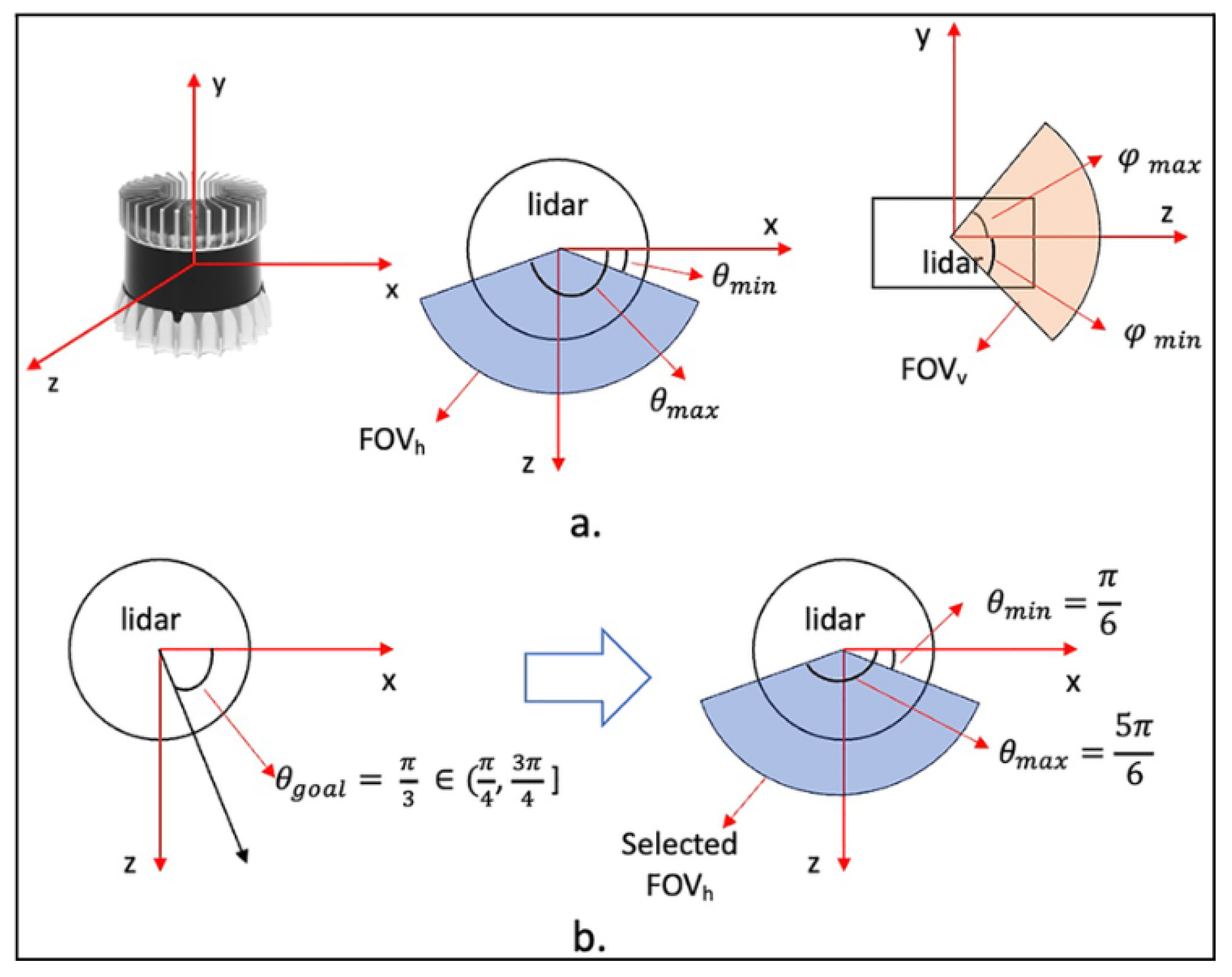
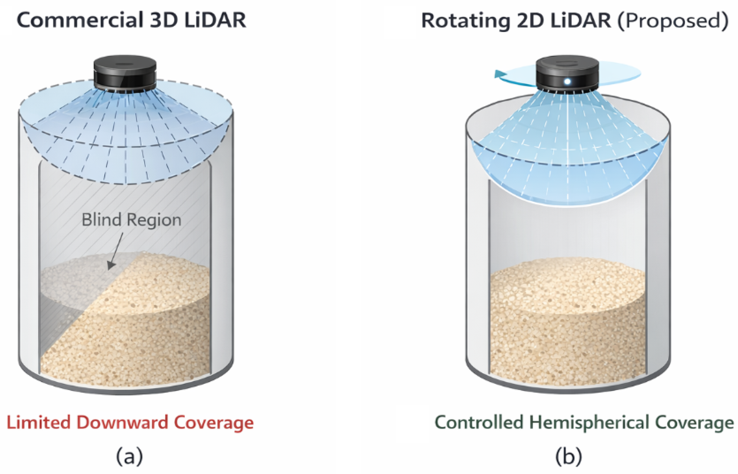
To contextualize the geometric limitations outlined in Table 2, a quantitative comparison further justifies the proposed system’s architecture. Commercially available 16-channel 3D LiDARs typically incur hardware costs exceeding > $4000. Furthermore, due to their limited vertical field of view (e.g., ± 15 ° ), a single commercial 3D LiDAR mounted at the top of a silo leaves significant blind spots near the bin walls. As a result, the estimated volumetric calculation errors exceed 10% unless multiple sensors are deployed and calibrated together—a process that increases deployment time to several days. In contrast, the proposed system utilizes modular, low-cost components, including a YDLiDAR X4, a Raspberry Pi 4, and an AX-12A servo motor, keeping the total hardware expenditure under $300. By mechanically sweeping the 2D LiDAR, the system guarantees full hemispherical coverage. Maintenance is equally streamlined; a mechanical failure in a dusty environment requires only the modular replacement of a $45 servo or $90 2D LiDAR, rather than the complete factory replacement required by sealed commercial 3D units. In addition, the proposed system adopts a structured scanning strategy based on controlled rotation of a 2D LiDAR. The resulting hemispherical coverage geometry is illustrated in Figure 1.
To visually illustrate the geometric limitations summarized in Table 2 and the motivation for the proposed sensing strategy, Figure 2 conceptually compares the effective sensing coverage of a commercial 3D LiDAR and the rotating 2D LiDAR adopted in this work. While mechanically rotating a 3D LiDAR could theoretically increase vertical coverage, such a configuration introduces substantial redundancy, mechanical complexity, and inefficient data utilization without resolving the fixed beam geometry inherent to commercially available 3D LiDAR systems. These limitations are particularly pronounced in enclosed volumetric measurement tasks, where sensing geometry must be tightly aligned with the measurement environment.
As summarized in Table 1, most commercial 3D LiDAR systems are optimized for wide-area environmental perception and exhibit the following constraints when applied to flour bin volume measurement:
  • Limited vertical field of view, restricting downward-focused sensing;
  • Fixed beam elevation angles, preventing adaptive hemispherical coverage;
  • Inefficient data utilization, with a large portion of emitted beams intersecting walls or non-relevant regions;
  • High cost and bulky form factor, limiting practical industrial deployment;
  • Increased integration and calibration complexity, especially in enclosed storage containers.
To address these constraints, the proposed system adopts a rotating two-dimensional LiDAR configuration, as illustrated in Figure 2. The design achieves the required sensing geometry through structured motion rather than increased sensor dimensionality, offering several advantages:
  • Controlled hemispherical coverage tailored to vertical bin geometry;
  • Uniform sampling density across the granular surface;
  • Geometry-aware surface reconstruction constrained by silo boundaries;
  • Efficient data acquisition with minimal redundant measurements;
  • Cost-efficient and deployable system design suitable for industrial facilities.
By prioritizing scan geometry suitability and structured motion, the proposed approach enables accurate volumetric measurement in enclosed flour storage bins while mitigating the limitations associated with both static and mechanically rotated 3D LiDAR systems.

2. Materials and Methods

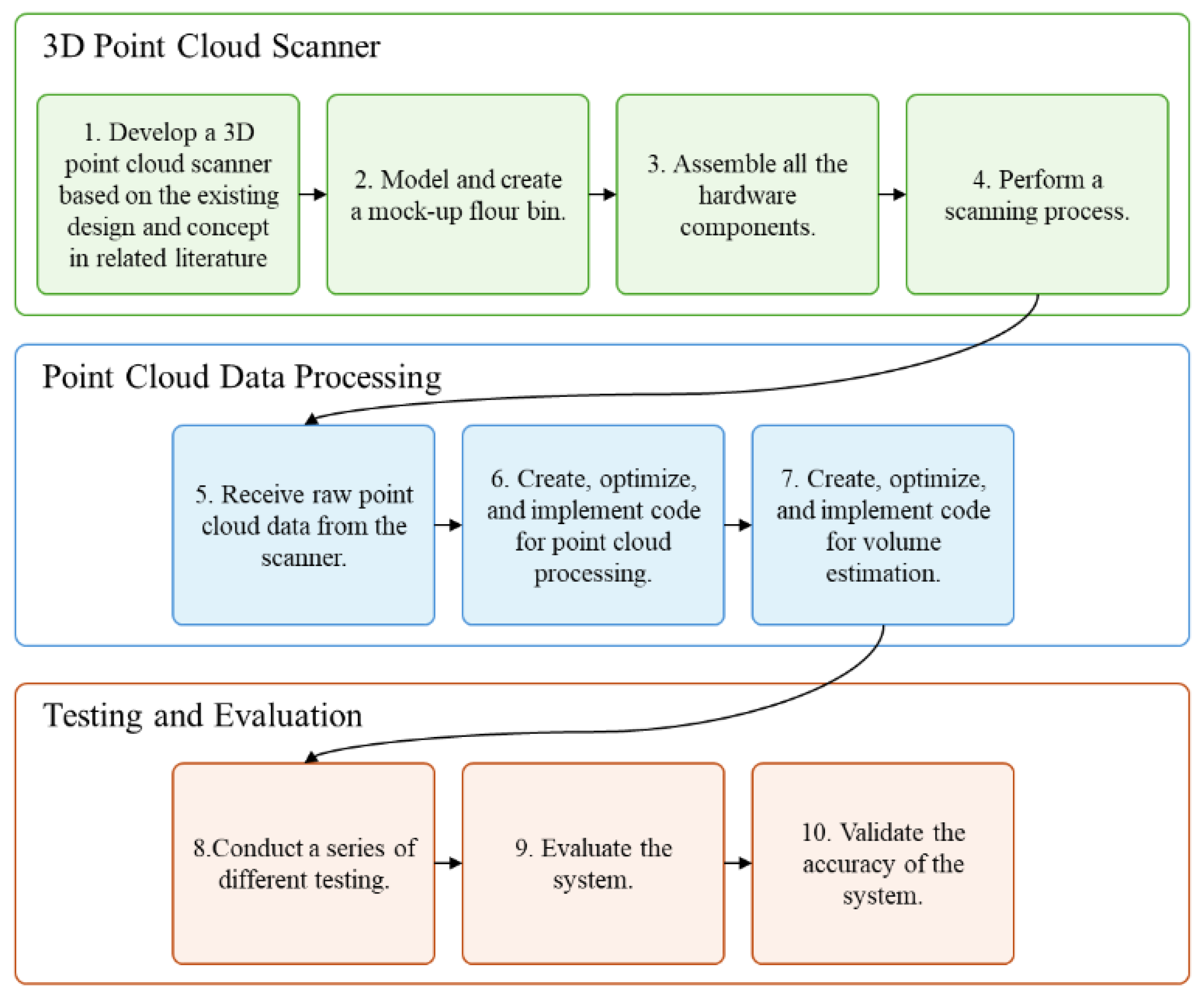
Accurate and efficient post-harvest processes are vital in the food industry to ensure effective inventory management and maintain an adequate supply of materials. Automation with remote sensing devices, modern technologies that can be integrated into a variety of industries, eliminates labor-intensive processes that may expose employees to dangerous scenarios. However, when flour is involved, dust clouds can form inside the bin during scanning, potentially leading to inaccurate data from the 3D point cloud scanner. Such inaccuracies can impact subsequent processing of the point cloud data. Figure 3 illustrates the general conceptual flow of the 3D point cloud scanning, processing, and evaluation system.
The research is based on the idea of using automation for industrial operations, specifically in the food industry. Point cloud data is a collection of an unorganized set of x, y, and z coordinates in a three-dimensional space. There are various ways to acquire point cloud data, and one possible way is through active non-contact sensing technology such as LiDAR sensor. LiDAR uses Time-of-Flight (TOF) methods of measuring the distance between the sensor and the object. TOF scanners are inexpensive compared to other specialized 3D scanners [34]. Researchers utilize LiDAR to acquire 3D point cloud data because of its ability to gather data and convert it into a global world coordinate frame [35]. This study does, however, acknowledge the potential limitations of LiDAR: when the environmental medium (water vapor, gases, dust particles) obstructs the target surface, the precision of the LiDAR-acquired point cloud data may be altered [34]. Thus, the researcher will manage the raw point cloud data by filtering the interfering elements such as dust. Lastly, Delaunay triangulation is a computational geometry computation that connects a set points to form a mesh of triangles. It can be used for volume estimation by calculating the volume of a convex hull [36,37], which will be used in this study.
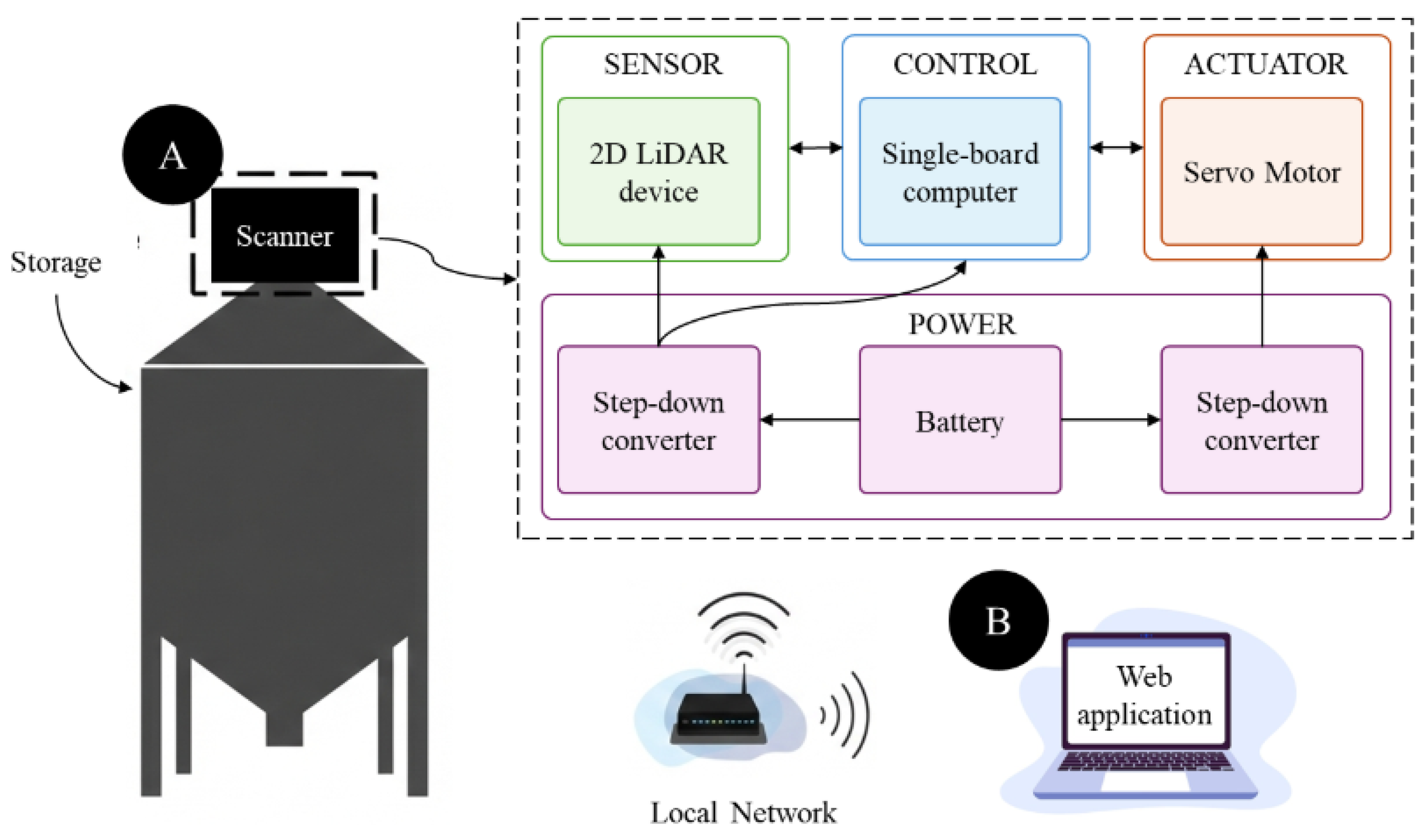
Figure 4 shows the system architecture of the the 3D Point Cloud Scanner System comprising a 2D LiDAR sensor, single-board computer, and servo motor, all powered by a battery regulated with a buck converter. The flow chart in Figure 3 outlines the development process of the Web-Based 3D Point Cloud Scanner System and Web Application, where each phase is essential for shaping the overall system’s functionality.

2.1. Hardware Integration

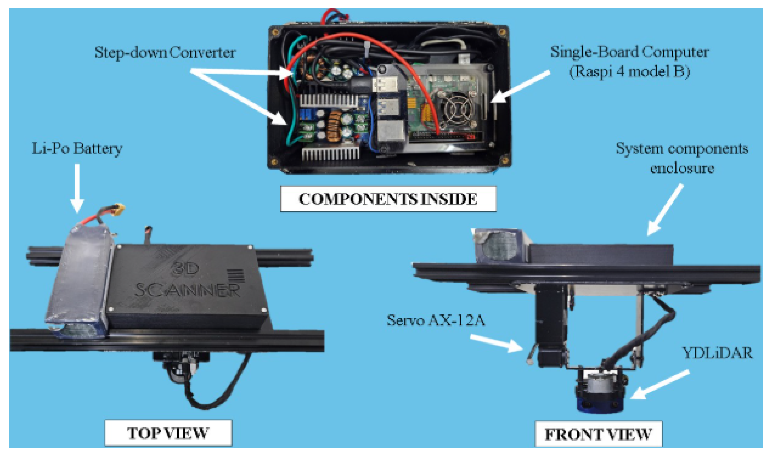
As illustrated in Figure 5, the hardware architecture of the 3D Point Cloud Scanner System (3D-PCSS) consists of a 2D LiDAR sensor, a rotating mechanism driven by a servo motor, and a single-board computer. The hardware requirements for the 2D LiDAR scanning subsystem were established based on three essential functional criteria:
  • A 2D LiDAR device capable of scanning within a horizontal field of view of at least 180°;
  • A minimum measurable range of 10 m to accommodate varying bin dimensions;
  • A single-board computer equipped with a 64-bit CPU operating at a minimum of 1.8 GHz, at least 4 GB of RAM, 5 GB of available disk space, and full compatibility with the required operating system and software libraries.
The rotating mechanism integrated with 2D LiDAR follows the methodology described by [25], which provides the foundational framework for using a pan–tilt unit (PTU) to transform planar scans into three-dimensional point cloud data. Guided by this previous work, the rotating device was designed with two operational requirements: it must rotate through an angular sweep of 0° to 180°, and it must maintain high positioning precision with an angular resolution finer than 1°. These specifications ensure accurate spatial sampling and reliable reconstruction of the bin’s interior geometry.
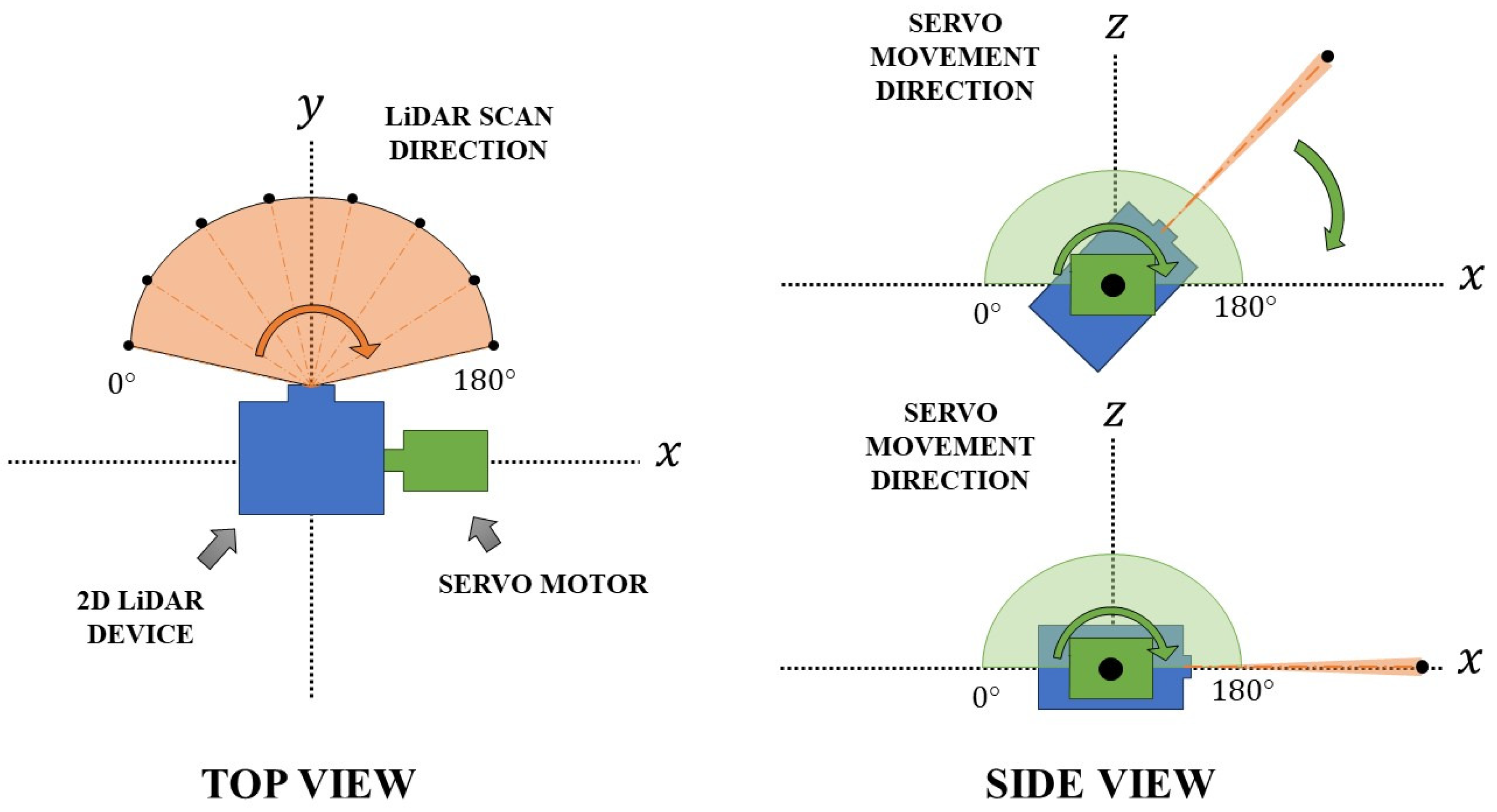
Figure 6 provides an illustration of the attachment of the servo to the 2D LiDAR device, enabling an additional axis of movement. It also demonstrates the respective scan angle directions of the LiDAR and the movement direction of the servo motor. After the LiDAR scans from 0 to 180°, the system sends a command to the servo to move to the next angle until it reaches the end angle.
  • The rotating device can rotate a minimum angle from 0 of 180 degree.
  • The rotating device has a minimum angular resolution of ≤1 degree.
Figure 7 provides an illustration of the servo’s attachment to the 2D LiDAR device, enabling an additional axis of movement. It also demonstrates the respective scan angle directions of the LiDAR and the movement direction of the servo motor. This synchronization method is further detailed in Algorithm 1. After the LiDAR scans from 0 to 180 degrees, the system sends a command to the servo to move to the next angle until it reaches the end angle.
Algorithm 1: Synchronization of LiDAR and Servo
Input: Initialized LiDAR sensor lidar, Servo motor servo
Output: Synchronized LiDAR scan data at discrete servo positions
1 
Initialize LiDAR and Servo;
2 
repeat
3 
   Start LiDAR scan from 0 ° to 180 °
4 
   while LiDAR scan is not complete do
5 
      Wait for scan to complete;
6 
   if LiDAR scan is complete then
7 
      if Servo is at final position then
8 
         Terminate the process;
9 
      else
10 
         Send command to Servo to move to next position;
11 
until servo reaches the final position;
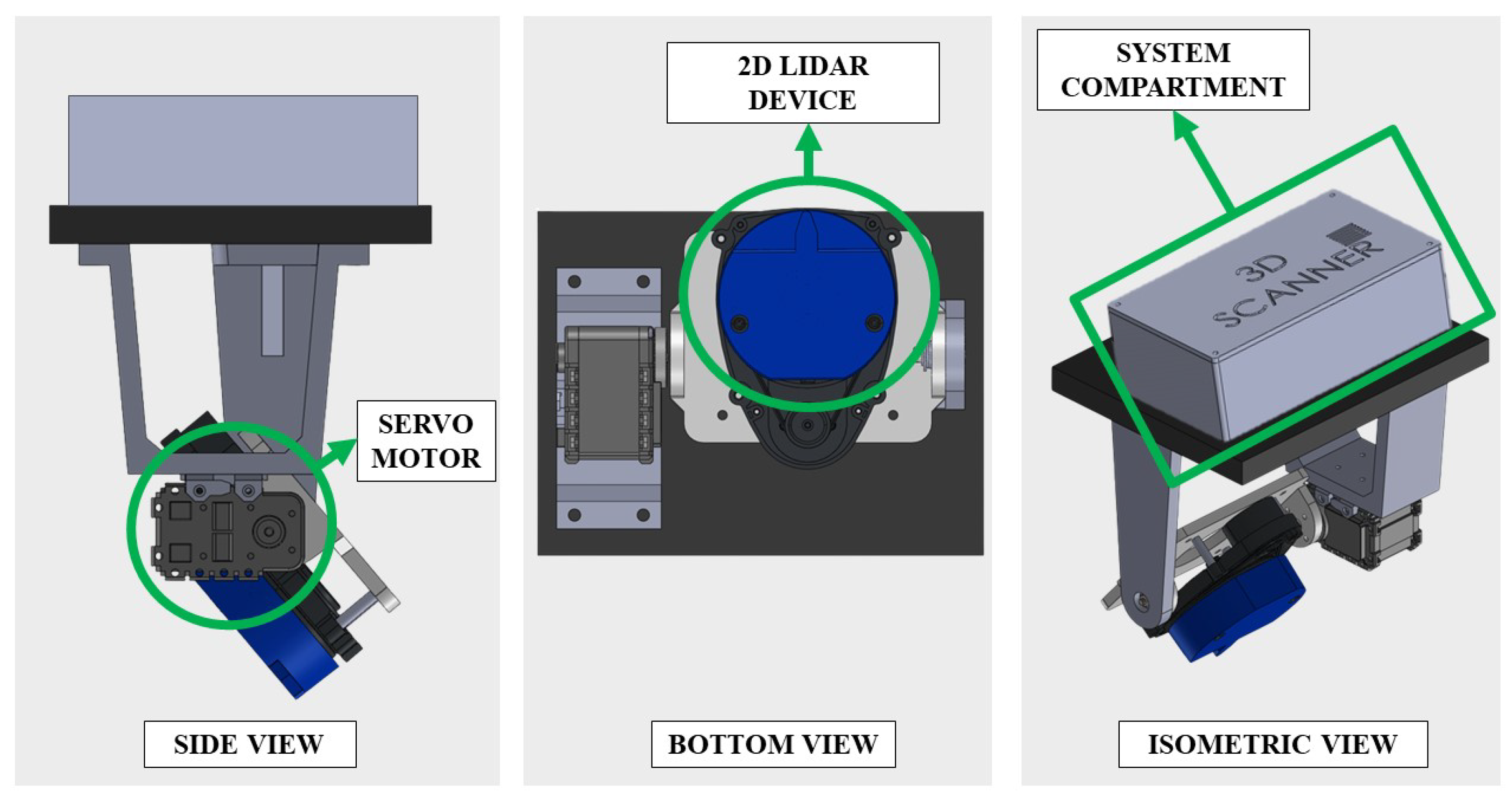
Figure 7, Figure 8 and Figure 9 illustrate the complete mechanical and electrical integration of the 3D Point Cloud Scanner System. Figure 5 presents multiple CAD views of the enclosure, showing the arrangement of the primary components: the side view emphasizes the mounting of the AX-12A servo motor responsible for the rotational motion of the LiDAR, the bottom view reveals the placement of the YDLiDAR X4 sensor, and the isometric view provides a full visualization of the assembled system and its compartment layout. Regarding angular accuracy, the proposed system employs controlled incremental rotation with calibration and synchronized data acquisition, which limits cumulative angular error during scanning. The resulting point clouds were verified through repeated scans, showing stable reconstruction performance for the intended volumetric measurement task.
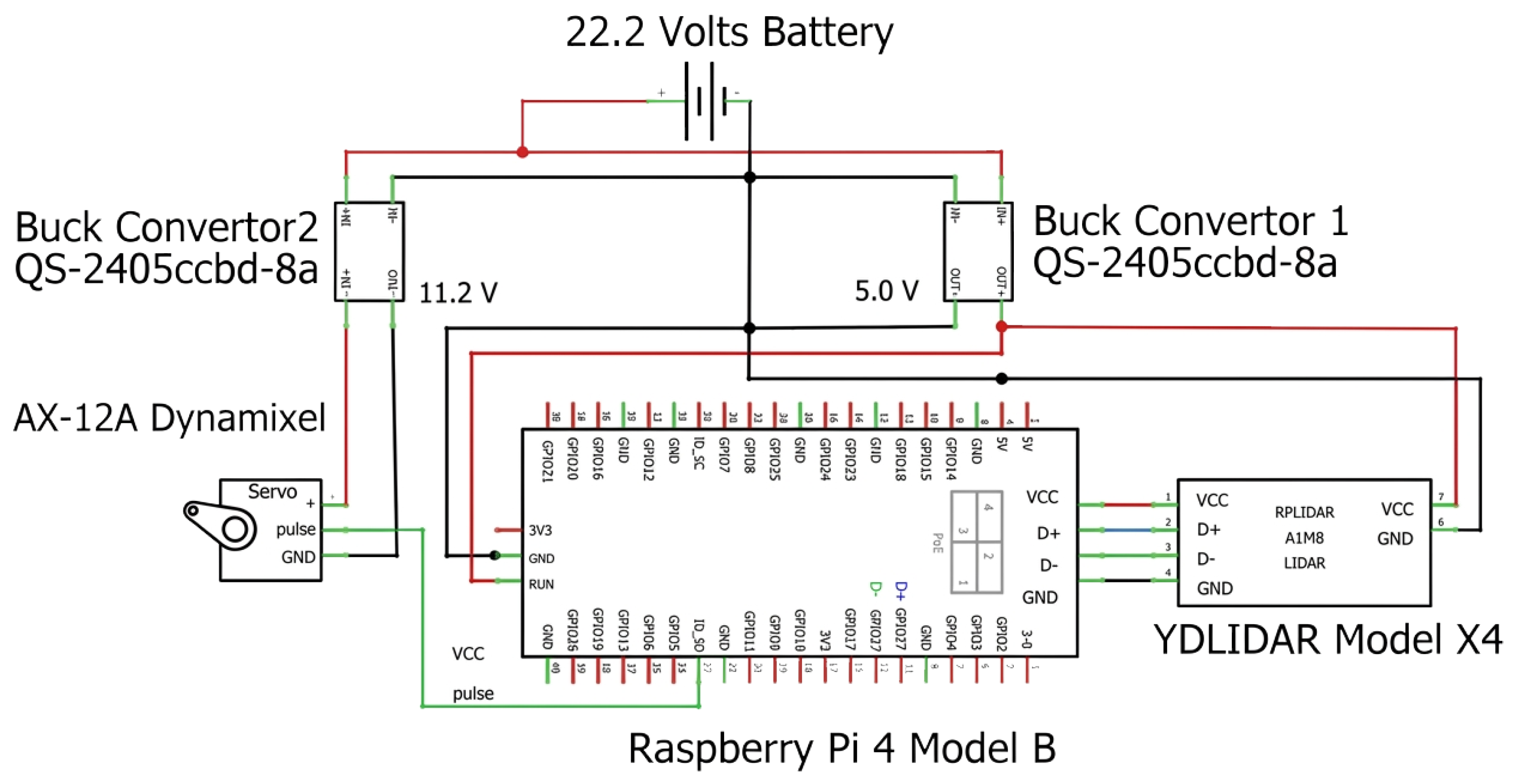
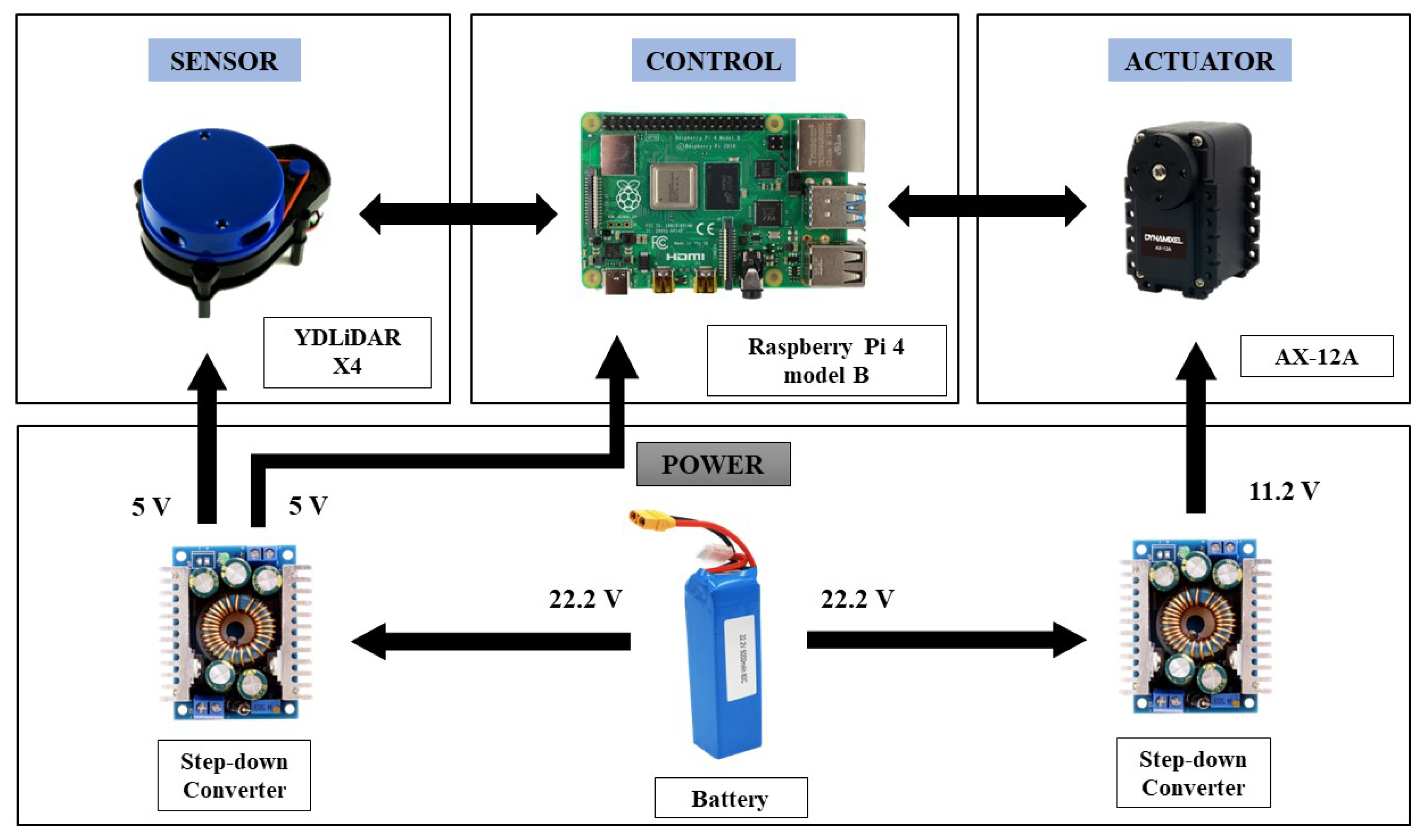
Figure 8 details the core hardware elements, including the YDLiDAR X4 for range sensing, the Raspberry Pi 4 Model B for system control and data processing, and the AX–12A actuator for vertical rotation. Figure 9 presents the overall circuit diagram, where a 22.2 V battery serves as the main power source and is regulated by two buck converters: one decreases to 11.2 V to drive the AX–12A Dynamixel and another supplies 5 V to the Raspberry Pi 4 Model B and YDLiDAR X4. Concerning reliability in dusty environments, the system was designed and tested under real flour silo operating conditions, including the presence of dust during filling. The mechanical components were enclosed, and experimental results demonstrated stable operation throughout the measurement period, indicating suitability for practical deployment. Although long-term degradation is a valid consideration, the focus of this study is on feasibility and performance validation under real-world conditions rather than lifetime endurance testing. With respect to accuracy, the goal of this work is not to replace high-end commercial 3D LiDAR sensors, but to provide a low-cost alternative for industrial volume estimation. Experimental results show that the proposed 2D LiDAR-based system achieves consistent and application-appropriate accuracy for flour bin volumetric measurement, validated against known bin geometry and reference volume calculations. These results demonstrate that the simplified hardware setup is sufficient for the targeted application.

2.2. Software Development

The software architecture of the 3D Point Cloud Scanner System was developed using the Robot Operating System, ROS version 1 Noetic Ninjemys, running on Ubuntu 20.04 LTS, following a modular, distributed, and event-driven design. Multiple ROS nodes manage sensor data acquisition, motor control, point cloud mapping, volume computation, and user interaction via a web interface. The system was developed and tested on an ASUS TUF FX505DU laptop equipped with an AMD Ryzen™ 7 3750H processor (up to 4.0 GHz), 16 GB DDR4 RAM, 512 GB NVMe SSD, 1 TB HDD, and an NVIDIA GeForce GTX 1660 Ti (6 GB GDDR6) GPU.

2.2.1. ROS Node Architecture

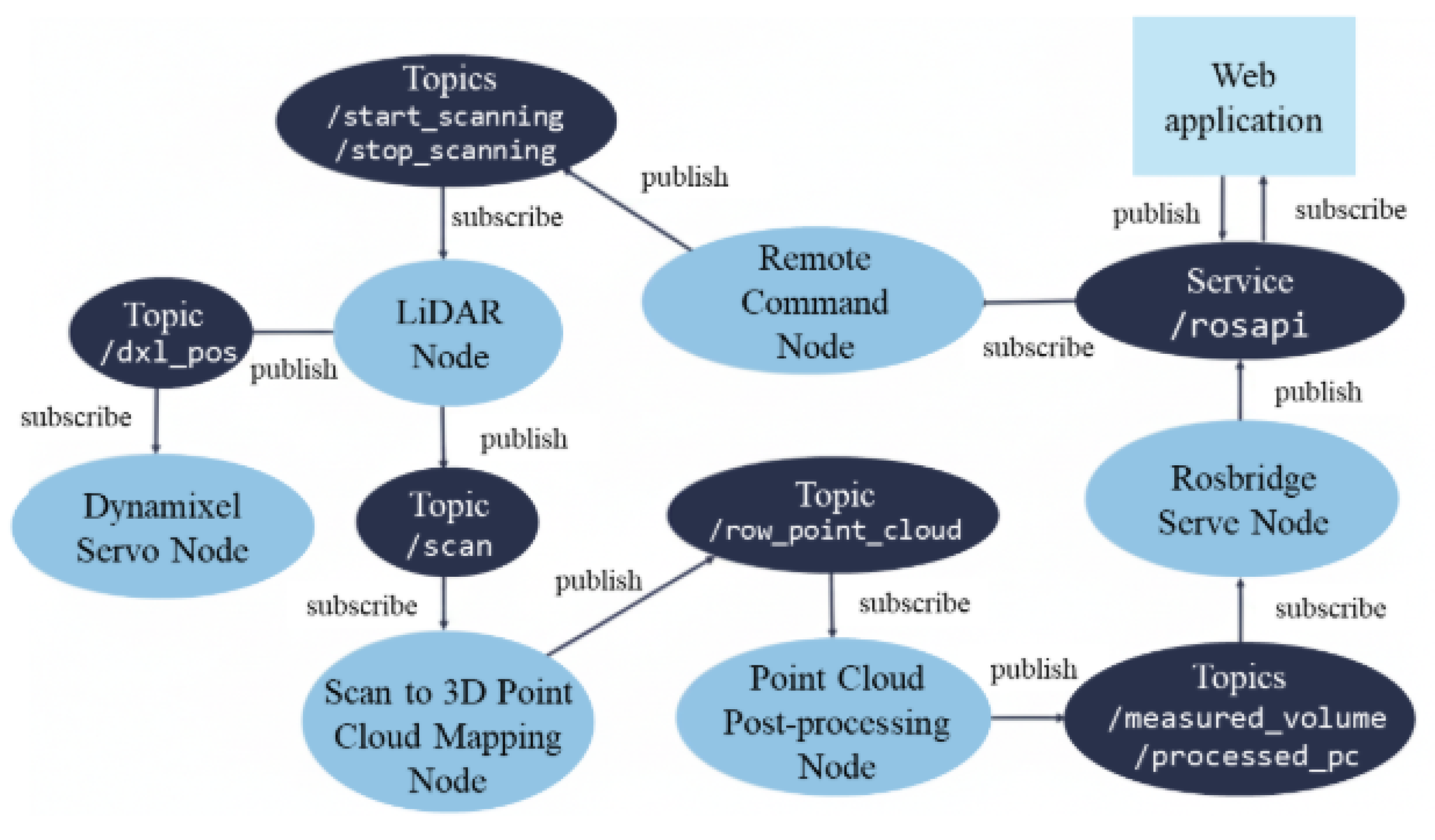
The system’s software functionality is divided into several ROS nodes, which communicate through topics in a publish–subscribe model. In this communication architecture, each node operates independently and exchanges information through topics: a node acting as a publisher transmits data to a topic, while other nodes acting as subscribers receive that data without direct dependency. This decentralized design ensures modularity and efficient data flow between system components. Each node is responsible for a specific function, such as LiDAR data collection, servo motor positioning, scan-to-point cloud conversion, and volume calculation. The overall ROS communication structure among these nodes is illustrated in Figure 10.
The LiDAR node is responsible for capturing 2D range data from the YDLiDAR X4 sensor and publishing the measured distances in real time. The servo node manages the angular position of the servo motor that tilts the LiDAR sensor, updating its orientation for each scan cycle. The command node listens for user commands transmitted via WebSocket from the web interface, initiating and controlling the scanning process as required. The point cloud mapper synchronizes LiDAR data with servo angle readings to generate three-dimensional point cloud coordinates representing the surface geometry of the flour inside the storage bin. Finally, the volume estimator processes the resulting point cloud data and calculates the total volume using the convex hull algorithm, which determines the smallest enclosing 3D shape that represents the material’s surface boundary.

2.2.2. Data Processing Flow

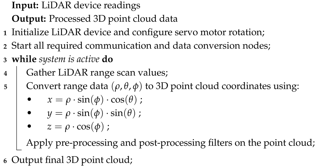
Upon receiving a scan command, the system enters active mode. The servo rotates incrementally, and the LiDAR captures horizontal scans at each step. Each range measurement ρ in meters and the corresponding angles θ and ϕ in degrees are recorded. These polar measurements are then converted into Cartesian coordinates—where x, y, and z represent the point’s horizontal, lateral, and vertical positions in meters—using the transformation equations shown in Equations (1)–(3). This conversion enables the construction of a complete 3D point cloud of the bin’s interior:
x = ρ cos ( ϕ ) cos ( θ )
y = ρ cos ( ϕ ) sin ( θ )
z = ρ sin ( ϕ )
The entire data processing flow consists of four key processes: preparing the operating system and framework, executing the bootstrap program, scanning and generating the point cloud, and measuring the volume. To ensure fully automated operation, a custom system service is configured to automatically launch core ROS services (roscore and rosbridge_server) during system boot. Once these services are initialized, the system transitions into an idle state, ready to receive and execute external commands through the web interface.

2.2.3. System Scanning Process

In the conceptual framework shown in Figure 3, the system is placed at the top of the storage bin. Once the system receives a command from the web application, it will start scanning the inside of the storage bin and acquiring range values from the LiDAR; otherwise the system will enter idle mode. The study developed ROS nodes that handle different processes such as initialization of the LiDAR device and servo motor, establishing a publish–subscribe relationship between these devices, and the conversion of LiDAR range scan data to point cloud data. The servo motor used in this study is compatible with a Software Development Kit (SDK) version 3.7.51, which includes configurations for integration with the ROS. The raw scan data from the LiDAR typically includes range values of the return pulses. These range values enter different stages of pre-processes to be mapped in two- or three-dimensional Euclidean space to create point cloud data and use for further post-processing.
The flow of processes from initialization to mapped point cloud data is listed in Algorithm 1. The method used in this study to process the range values gathered from the LiDAR device is described in the Algorithm 2, which was discussed in the theoretical framework. ρ represents distance from the origin (0,0,0) which is in our case the LiDAR, and this distance is measured in meters. The angle θ is the rotation around the z-axis in the xy-plane. The angle ϕ is the tilt of the radius vector from the positive z-axis: from 0 degrees on the positive z-axis down to 90 degrees on the xy-plane and to 180° on the negative z-axis. Equations (1)–(3) show the conversion formulas for the Cartesian coordinates x, y, and z, respectively.
Algorithm 2: LiDAR Range to 3D Point Cloud Mapping Process
 Technologies 14 00401 i001

2.2.4. Volume Measurement Process

An empty-space approach was used to measure the flour materials inside the storage bin. A simple representation of an empty-space approach is made following the concept discussed in the conceptual framework, as shown in Figure 3, where the 3D Point Cloud Scanner System is placed at the top of the storage bin to scan the empty space and generate point cloud data. This point cloud data is processed to calculate the empty-space volume using the convex hull method, specifically utilizing the Quickhull algorithm. The Quickhull algorithm computes the convex hull of the gathered point cloud data, enabling volume estimation. Theoretically, as shown in Equation (4), the volume of flour materials is determined by subtracting the volume of the empty space from the bin’s maximum volume capacity, a commonly used method in these studies [25,38].
V f = V m a x V e m p t y
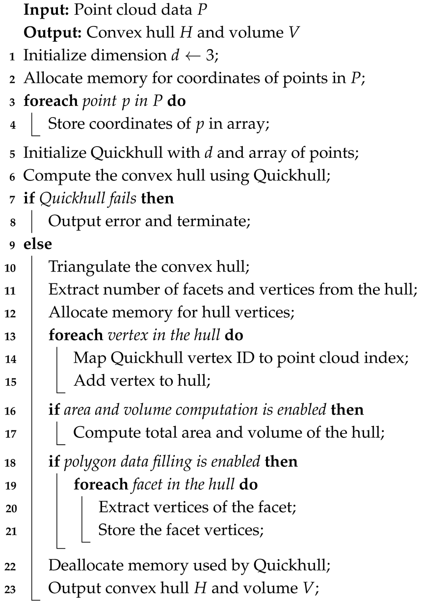
In Equation (4), V f represents the volume of the flour materials inside the bin, expressed in cubic meters ( m 3 ). The term V m a x denotes the maximum volumetric capacity of the flour bin, also measured in cubic meters ( m 3 ), based on its known geometric dimensions. Meanwhile, V e m p t y corresponds to the computed empty-space volume derived from the point cloud data, likewise expressed in cubic meters ( m 3 ). By subtracting the empty-space volume from the bin’s total capacity, the resulting value V f provides the estimated volume of flour stored at any given time. The raw data from the LiDAR is converted into point cloud data. This point cloud data can then use the convex hull to create a mesh for volume estimation. The Quickhull algorithm used for this process is shown Algorithm 3.
Algorithm 3: Quickhull Algorithm for 3D Point Cloud Volume Calculation
 Technologies 14 00401 i002

2.3. Web Application Design

The web application developed for the 3D Point Cloud Scanner System enables real-time, remote interaction by serving as the central interface for sending scan commands, visualizing point cloud data, monitoring system status, and storing measurement results.
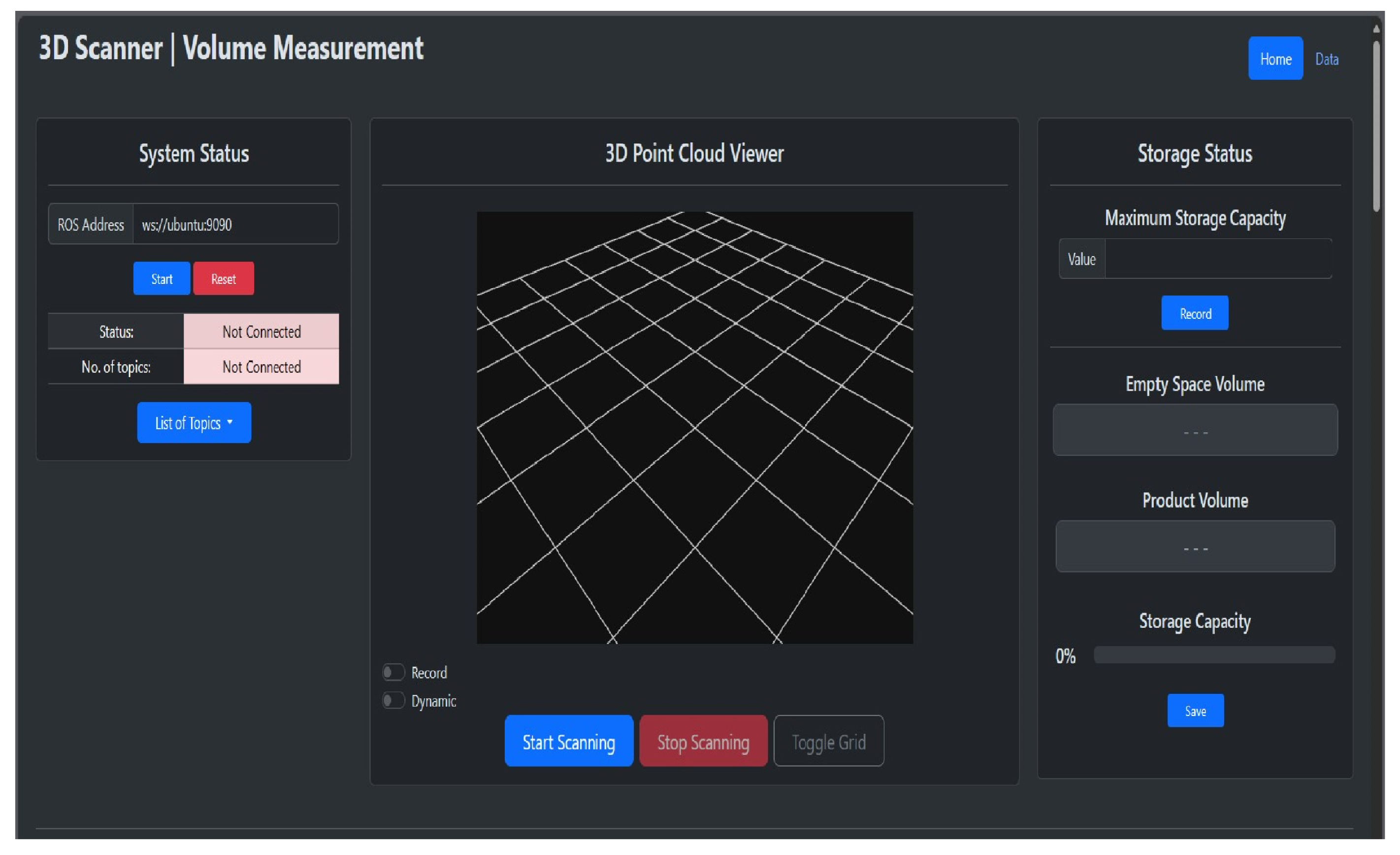
As shown in Figure 11, the web-based visualization platform integrates multiple frontend and backend components to provide real-time data communication, visualization, and user interaction. The system employs asynchronous communication mechanisms to facilitate efficient data exchange between the browser interface and ROS-based backend services. A WebGL-based rendering engine is utilized to display three-dimensional point cloud data directly within the browser, enabling users to inspect scanned bulk material surfaces without requiring specialized software. Integration with the Robot Operating System (ROS) allows seamless acquisition and visualization of sensor-generated data, including point clouds and measurement outputs. The platform incorporates dynamic charting capabilities to monitor volume estimation results over time, providing users with immediate feedback on system performance. A responsive user interface framework ensures compatibility across different devices and screen sizes, while an event-driven architecture coordinates interactions among system modules and maintains synchronized updates throughout the application.
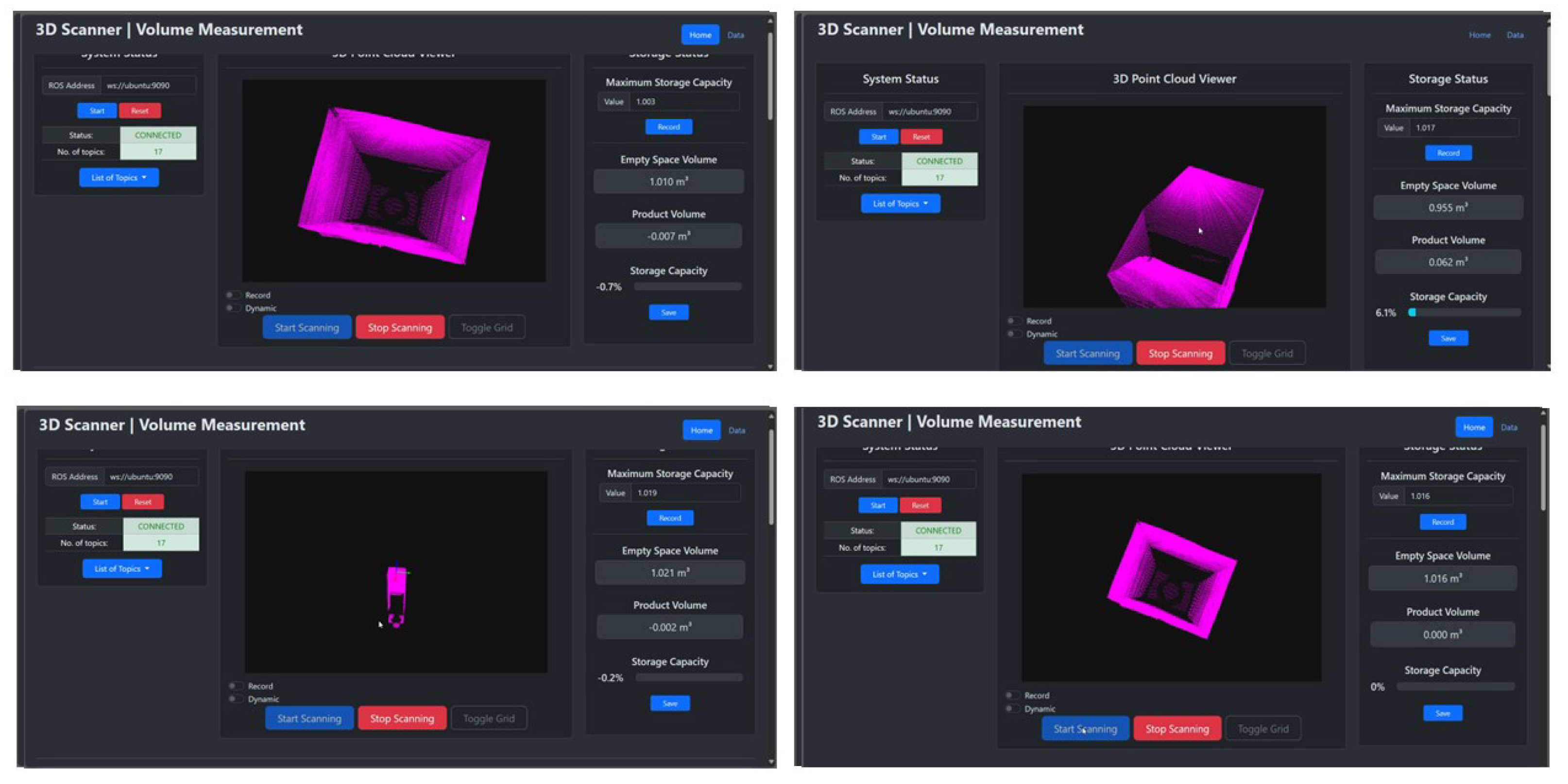
The web dashboard is organized into three main sections, as shown in Figure 11. The Left Panel provides system status information, including the current ROS connection state and a list of available topics. The Center Panel features an interactive 3D point cloud viewer that supports zooming, panning, and rotation, along with control buttons to start and stop scanning. Meanwhile, the Right Panel displays volume-related information such as current volume, empty space, and percentage capacity, and includes a save button for logging measurement data into the local database.
A local MySQL database was implemented to store volume measurement results, with schema containing fields for a unique ID, timestamp, empty-space volume, product volume, and overall storage capacity. After each scan, data entries are inserted directly through the web interface. Communication between the system and the web application is handled through a WebSocket protocol using rosbridge_server on the backend. The initialization of this communication involves a three-step handshake: the browser first sends a WebSocket upgrade request to the ROS bridge server; the server then accepts the request and responds with status code 101 (Switching Protocols); and, once confirmed, real-time bidirectional communication between the client and server is fully established.
This setup allows for low-latency interaction, ensuring a responsive and seamless user experience when monitoring live scanning sessions or controlling the system remotely.

2.4. System Testing and Calibration

This study conducted different tests and evaluations to observe the accuracy and performance of the overall system. The testing methods involved calibration tests and volume measurement tests of the system. The purpose of the LiDAR and servo calibration test was to adjust the accuracy of the range values recorded and the rotating angle of the servo motor, which is crucial for ensuring that the system accurately captures the spatial data necessary for generating precise 3D point clouds. The calibration testing setup was done in the laboratory room, where the range values of the LiDAR device were calibrated using a known reference distance. The LiDAR was positioned at various distances from the reference object, and the measured range values were compared against the known distances. Similarly, the angle of rotation of the servo motor was calibrated to ensure accurate positioning by commanding the servo to specific angles and verifying its actual position using a calibration tool, with any discrepancies between commanded and actual angles corrected through calibration adjustments. To mitigate the effects of Mie scattering caused by airborne flour particulates, all calibration and volume measurement tests were conducted under controlled environmental conditions. Specifically, scanning operations were initiated only after a mandatory settling period following any active filling or manual contouring of the flour. This ensured that airborne dust concentrations were kept to a minimum, which simulates the intended idle-state monitoring environment of the sensor.

2.4.1. System Volume Measurement Calibration Test

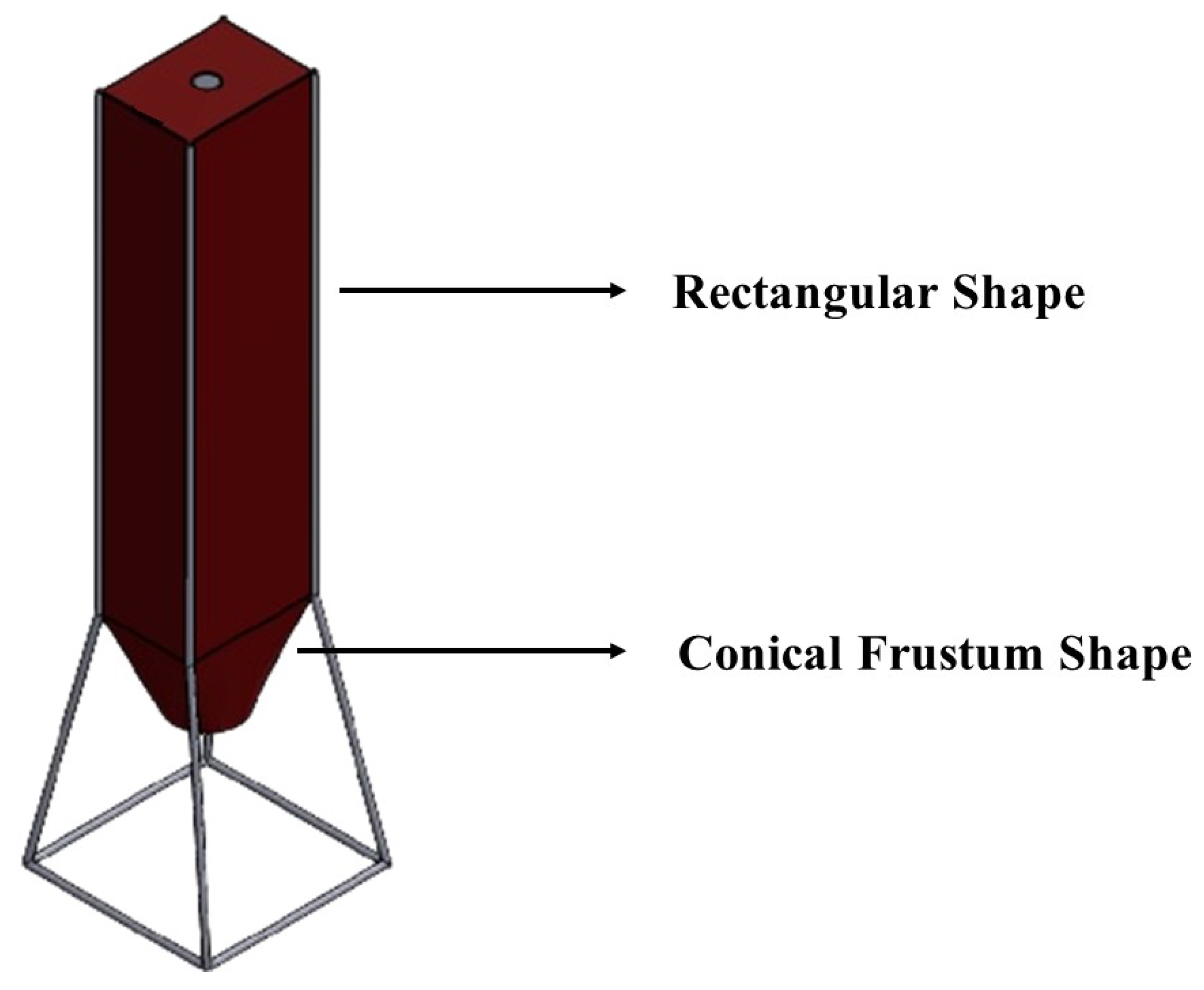
The calibration test was conducted to evaluate the accuracy and reliability of the 3D Point Cloud Scanner System in measuring volume across various scenarios. To achieve this, a mock-up flour storage bin was constructed to replicate the geometric characteristics of actual industry storage bins. As shown in Figure 12, the CAD model guided the physical build and consisted of a rectangular upper section and a conical frustum below it. The rectangular portion measured 2.5 m in height, 0.5 m in length, and 0.69 m in width. Attached beneath it, the conical frustum tapered from a top radius of 0.21 m to a bottom radius of 0.17 m, with a height of 0.42 m. This setup provided a controlled and representative environment for the calibration tests.
Before conducting different calibration test procedures, the system was calibrated and adjusted to minimize the error.

2.4.2. Empty Storage Volume Measurement Calibration

This calibration test involved performing multiple scans of an empty storage bin to measure its total volume. The purpose of this test was to scan the storage bin without any flour materials inside, ensuring an accurate baseline measurement. A total of exactly 30 independent scanning trials were conducted to establish a statistically significant baseline for the empty bin volume. Before starting the test, the actual total volume of the flour storage bin was manually measured and calculated based on its geometric shapes and dimensions using a steel tape measure with a resolution of 1 mm.

2.4.3. Different Volume Quantity Measurement Calibration

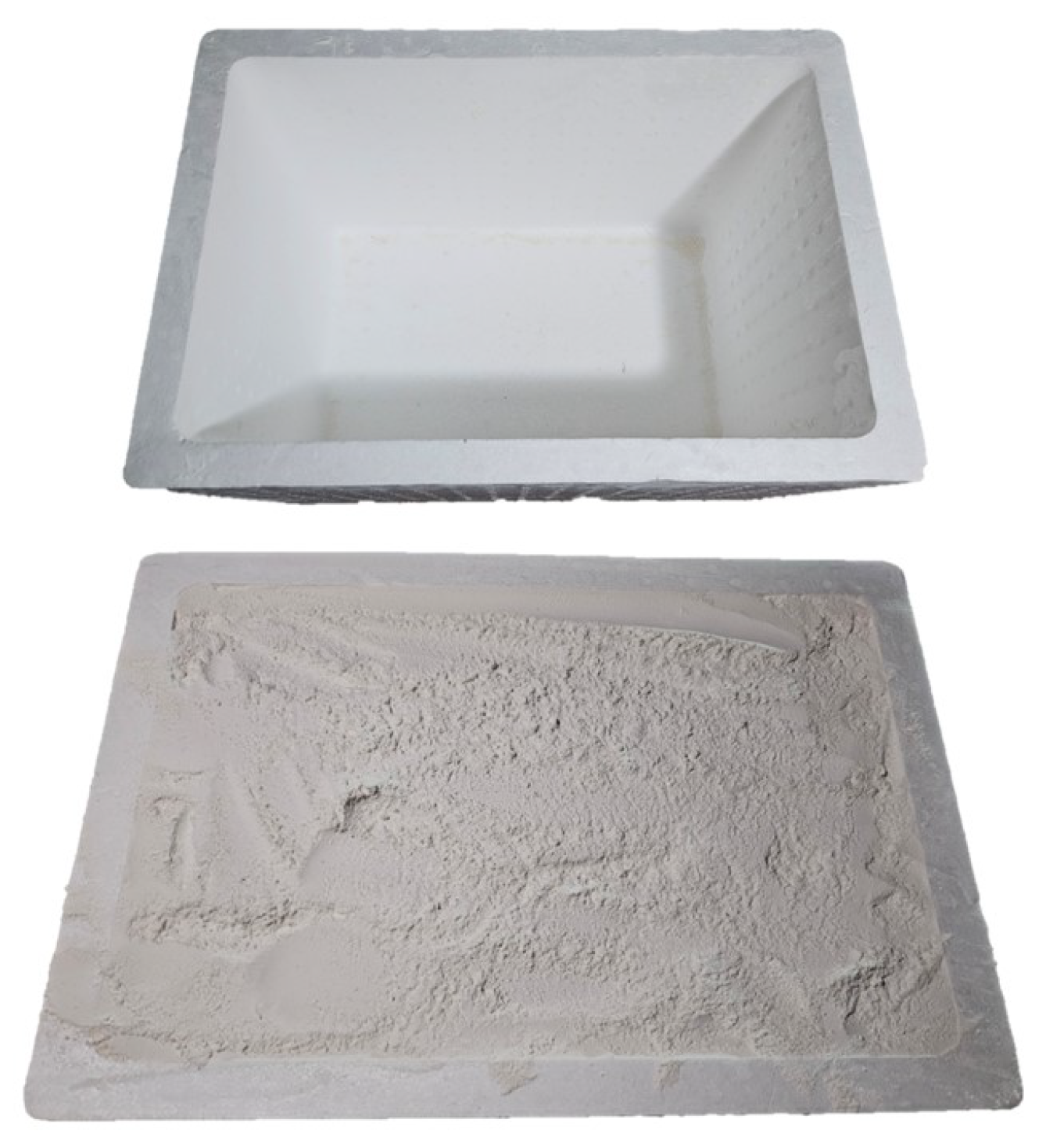
The calibration test involved filling the mock-up storage bin with different quantities of flour material to evaluate the system’s accuracy in measuring varying volumes. To ensure precise control and quantification, a white styrofoam box made of expanded polystyrene (EPS) with a known volume capacity of 0.0594 m3 was used to measure each batch of flour added. Three specific test volumes were prepared: the bin was first filled with 0.0594 m3 of flour, then with 0.4752 m3, and finally with 0.7128 m3. To evaluate measurement consistency, each of the three volume scenarios was tested using two distinct surface contours. For each specific contour, the system executed five independent scans, resulting in 10 scans per volume quantity and a total of 30 experimental scans across the varied quantity tests.

2.4.4. Volume Measurement Using the System and Sounding Method Test

To validate the accuracy and reliability of the 3D Point Cloud Scanner System, its volume measurements were compared with those obtained using the traditional sounding method. The traditional method involved manually measuring the flour depth inside the storage bin using a steel measuring tape with a 1 mm resolution and calculating the estimated volume based on the known geometric dimensions of the bin. For the experiment, the storage bin was filled with 0.0594 m3 of flour, and the flour surface was reshaped into five different contour profiles. For each contour shape, the volume was measured using both the proposed 3D scanning system and the traditional sounding method. In the manual approach, the depth measurements were converted to volume based on the bin’s geometry, while the proposed system computed volume directly from the generated point cloud. The resulting measurements from both methods were then recorded and compared to assess the system’s performance.

2.4.5. Measurement Error Analysis

To quantitatively evaluate the accuracy and reliability of the 3D Point Cloud Scanner System, three primary statistical error metrics were utilized: Mean Absolute Error (MAE), Mean Absolute Percentage Error (MAPE), and Standard Deviation (SD). MAE and MAPE were calculated to determine the absolute and relative deviations of the system’s estimated volumes against the manually measured reference volumes (ground truth). Standard deviation was computed across the repeated scanning trials to assess the system’s precision and measurement repeatability. Furthermore, a One-Sample t-test and ANOVA were utilized to determine if there were statistically significant differences between the proposed system’s measurements and traditional sounding methods.


3. Results

3.1. Actual Prototype of the 3D Point Cloud System

The actual developed 3D Point Cloud Scanner System was constructed according to the 3D CAD model design, shown in Figure 13. Before the integration of the system, individual component testing was conducted to test and verify if such components function properly. The base platform, to which the 2D LiDAR device and servo motor are attached, was fabricated using aluminum metal. The system compartment was 3D-printed.
3.2. Point Cloud to Measured Volume Processing Result

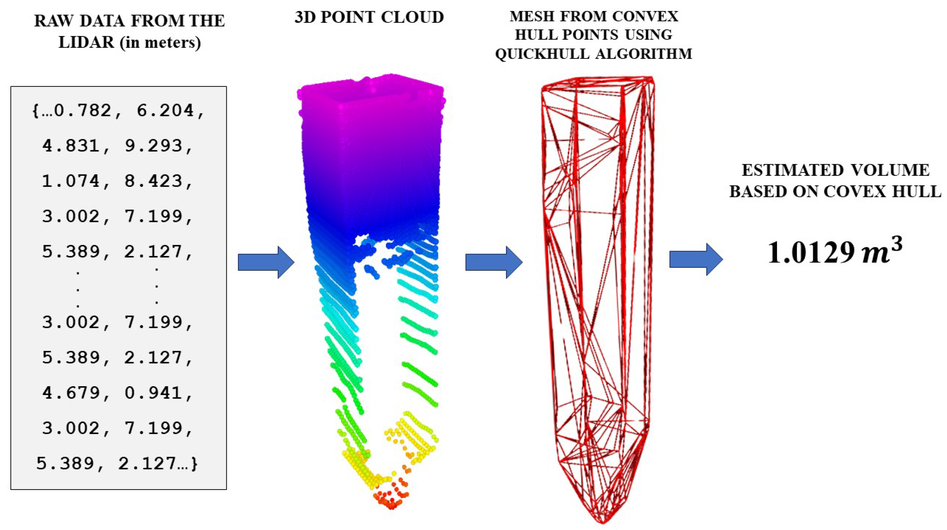
The processes of the system were implemented on the single-board computer (Raspberry Pi 4 model B), which serves as the central component driving the functionality of the 3D Point Cloud Scanner System. Figure 14 illustrates an example of the developed volume estimation process of the system. The algorithm processes the 3D point cloud by first initializing the necessary parameters, including setting the dimension to 3 and allocating memory for point storage. It then iterates through the point cloud to store all coordinates in an array. Using the Quickhull algorithm, it computes the convex hull of the point cloud, with appropriate error handling in case the computation fails. Once the hull is obtained, it is triangulated to enable accurate volume estimation. The algorithm then extracts and maps hull vertices, computes the area and volume if enabled, and optionally fills in polygon data for each facet. Finally, it deallocates all used memory and outputs the resulting convex hull along with the estimated volume.

3.3. System Testing and Evaluation

After conducting various tests, the performance of the 3D Point Cloud Scanner System was assessed. The evaluation covered both hardware and software components, as well as the integration of the web application. The hardware testing involved verifying the functionality of the LiDAR sensor and servo motor. The LiDAR was tested for scanning range, angular resolution, and distance accuracy, while the servo motor was evaluated for rotation and repeatability at different scanning angles. Software testing focused on the algorithms for data acquisition, point cloud generation, and volume estimation. The system was validated by comparing the estimated measurements against actual reference dimensions, ensuring that the generated 3D models accurately represented the scanned objects. Integration testing examined communication between hardware, software, and the ROS-based architecture. Publish–subscribe interactions among nodes were tested to confirm that data was transmitted and processed in real time without delays or loss. Finally, system evaluation included testing, where the entire setup, from LiDAR scanning to web-based visualization, was executed. User interaction through the web application was also tested to ensure accessibility and ease of use.

3.4. LiDAR and Servo Calibration Test Results

Five trials were conducted, with the LiDAR sensor capturing range data for five different reference points. The results of the calibration test are summarized in Table 3. The average measurements are very close to the actual ranges, and the low standard deviation (ranging from 0.0087 m to 0.0155 m) indicates high consistency and repeatability of the LiDAR readings across trials.
The servo angle calibration test focused on assessing the rotational accuracy of the servo motor, which determines the orientation of the LiDAR sensor during scanning operations. Similar to the LiDAR range calibration, five trials were conducted to evaluate the servo’s performance across various angular positions. The results of the calibration test are presented in Table 4.

3.5. System Volume Measurement Servo Calibration Result

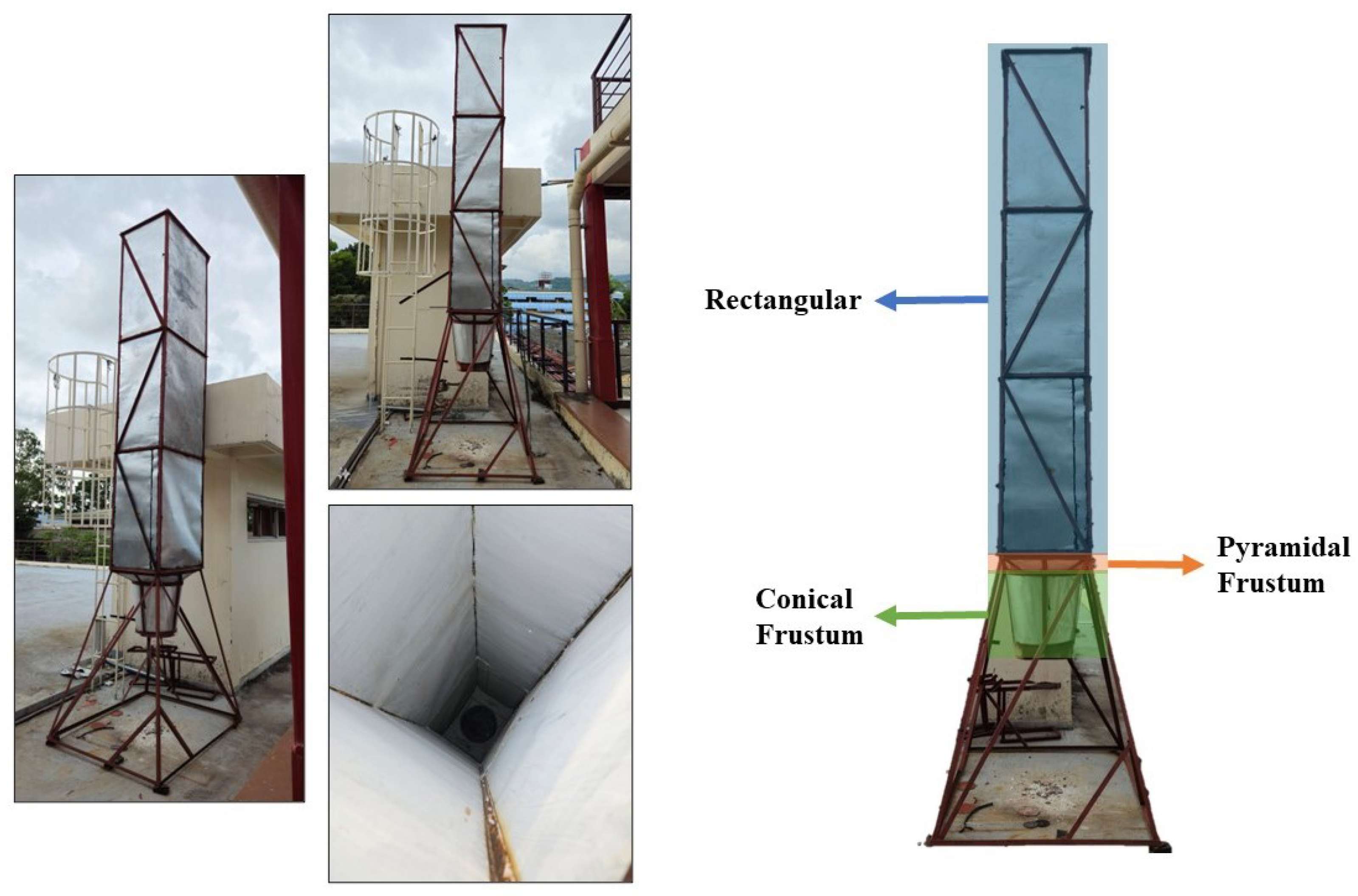
Different volume measurement calibration tests were conducted. The actual mock-up bin consists of three distinct geometric shapes as depicted in Figure 15. The dimensions of each shape were manually measured using a steel tape measure. The target object consists of three distinct geometric sections with the following dimensions: a rectangular base measuring 2.775 m in height, 0.5 m in length, and 0.69 m in width; a pyramidal frustum atop the base with an upper length of 0.5 m, upper width of 0.69 m, lower length and width of 0.42 m, and height of 0.03 m; and a conical frustum positioned at the topmost part, featuring a top radius of 0.21 m, bottom radius of 0.17 m, and height of 0.42 m. With these dimensions, the individual and total volume capacities of the storage bin were calculated. Table 5 provides a summary of the measured individual and total volume capacity of the bin.
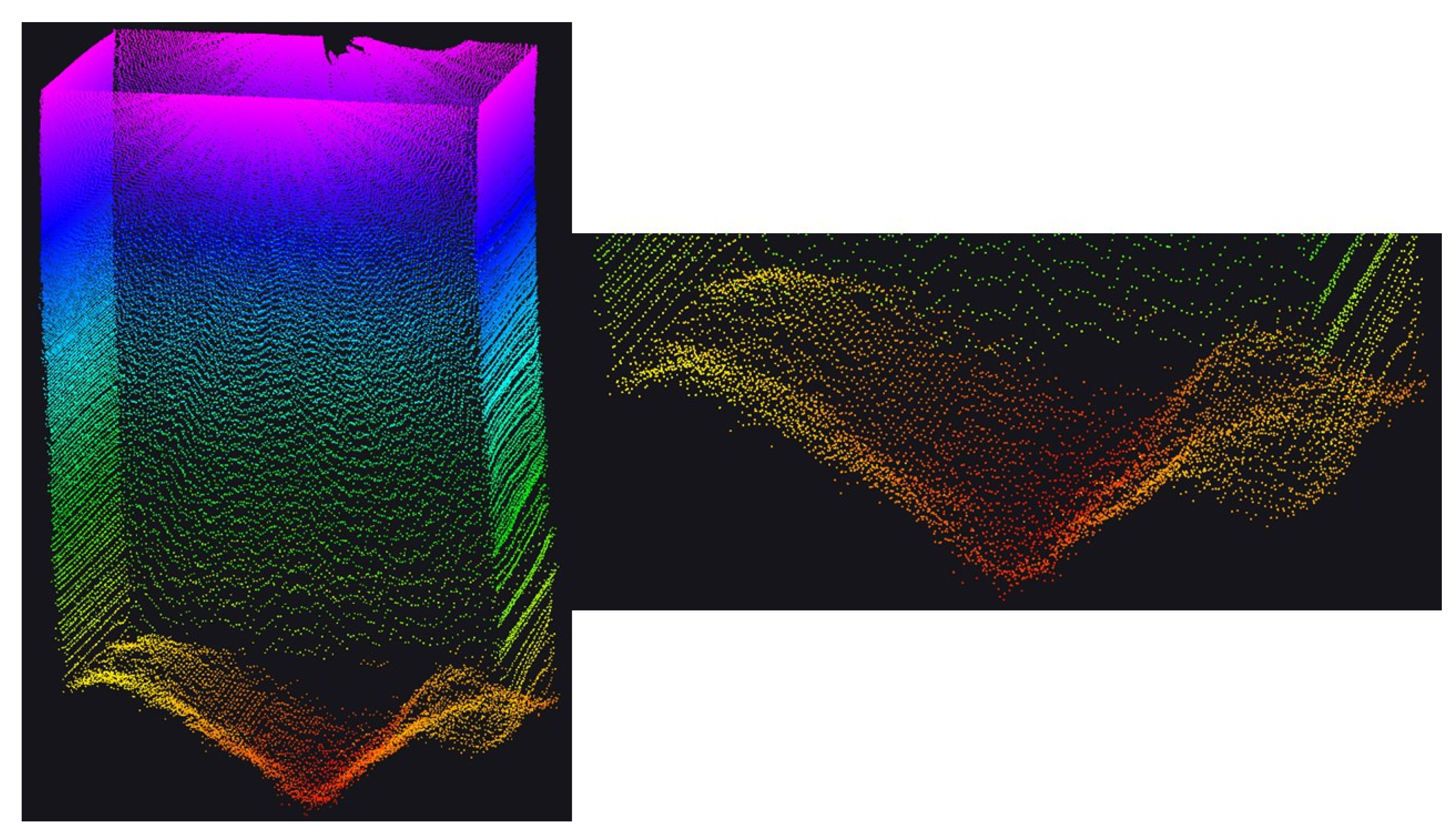
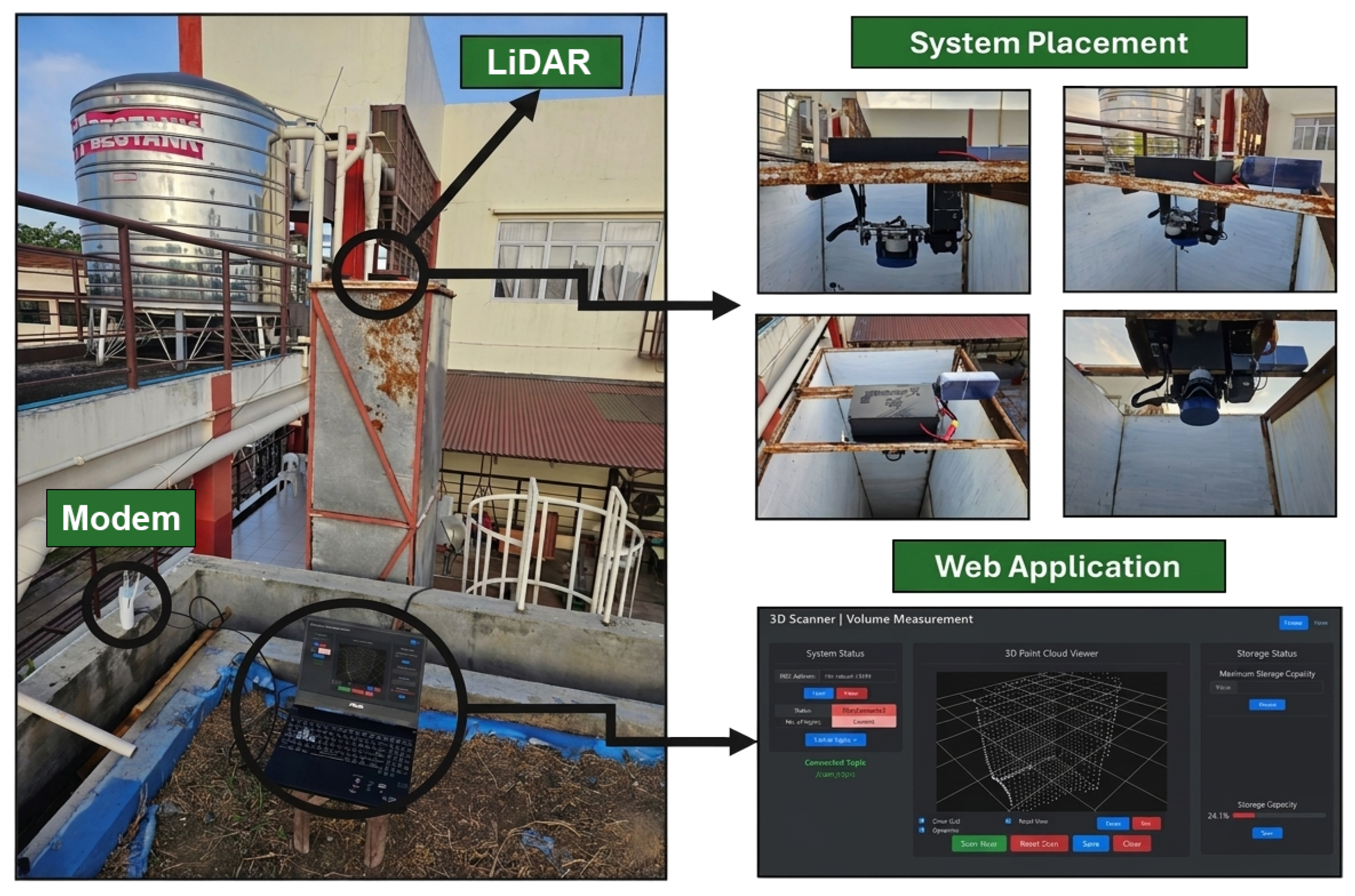
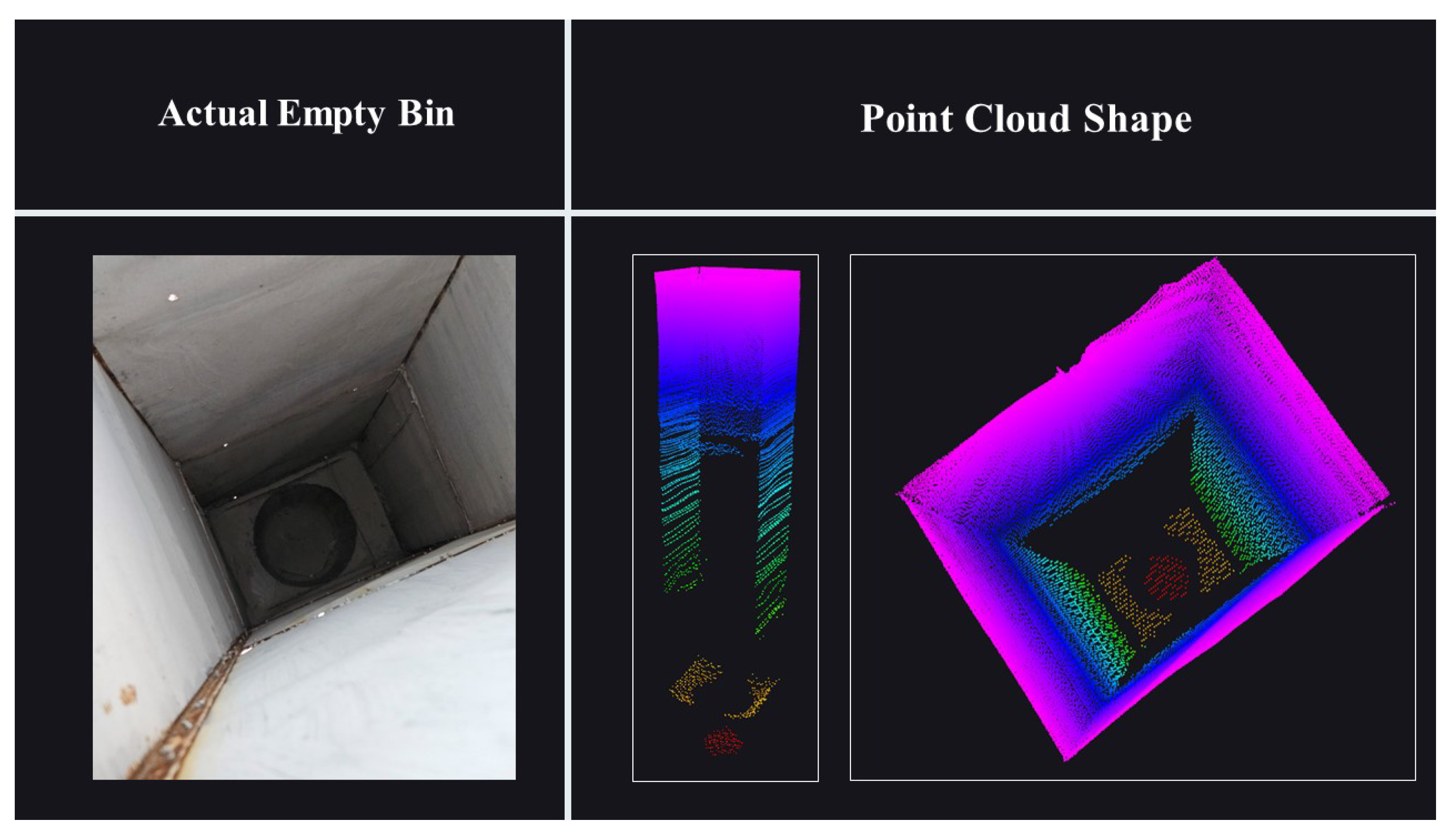
The actual field system setup shown in Figure 16 demonstrates the placement of the 3D Point Cloud Scanner System and the end-user device where the web application is running. The actual field testing took place within the university premises. Multiple scans and volume measurements of an empty storage bin were performed. Figure 17 shows the the sample point cloud scan of the system and the actual empty bin.
The actual visualization of the point cloud and volume is shown in Figure 18. Figure 19 shows the rendered 3D point cloud data from the scanner system and the equivalent convex hull volume in the created web application.
Based on Figure 18, the average measured volume of the system is 1.0128 m3, while the actual total volume of the storage bin is 1.0129 m3. To determine the actual volume of the storage bin, the study calculated the total volume it can store based on its dimensions and geometric volume. The absolute maximum error was found to be 0.0060 m3 and the absolute minimum error was 0.0020 m3. The resulting average error was 0.00014 m3 and is slightly under the actual volume of the storage bin. To determine whether it is statistically different from the mean total storage volume of 1.0129 m3 and the mean measured volume of the system, Table 6 presents the result of a One-Sample t-test. According to the p-value, which is above 0.05, shown in the table above, there was no statistically significant difference detected.

3.6. Different Volume Quantity Measurement Calibration Test Result

A container with a known volume was used throughout this test to fill the storage bin as shown in Figure 19. This container was measured manually and has a total volume capacity of 0.0594 m3. In this test, three different scenarios were conducted; the flour storage bin was filled with different volumes of flour materials: 0.0594 m3, 0.4752 m3, and 0.7128 m3.

3.6.1. Storage Bin Filled with 0.0594 m3 of Flour

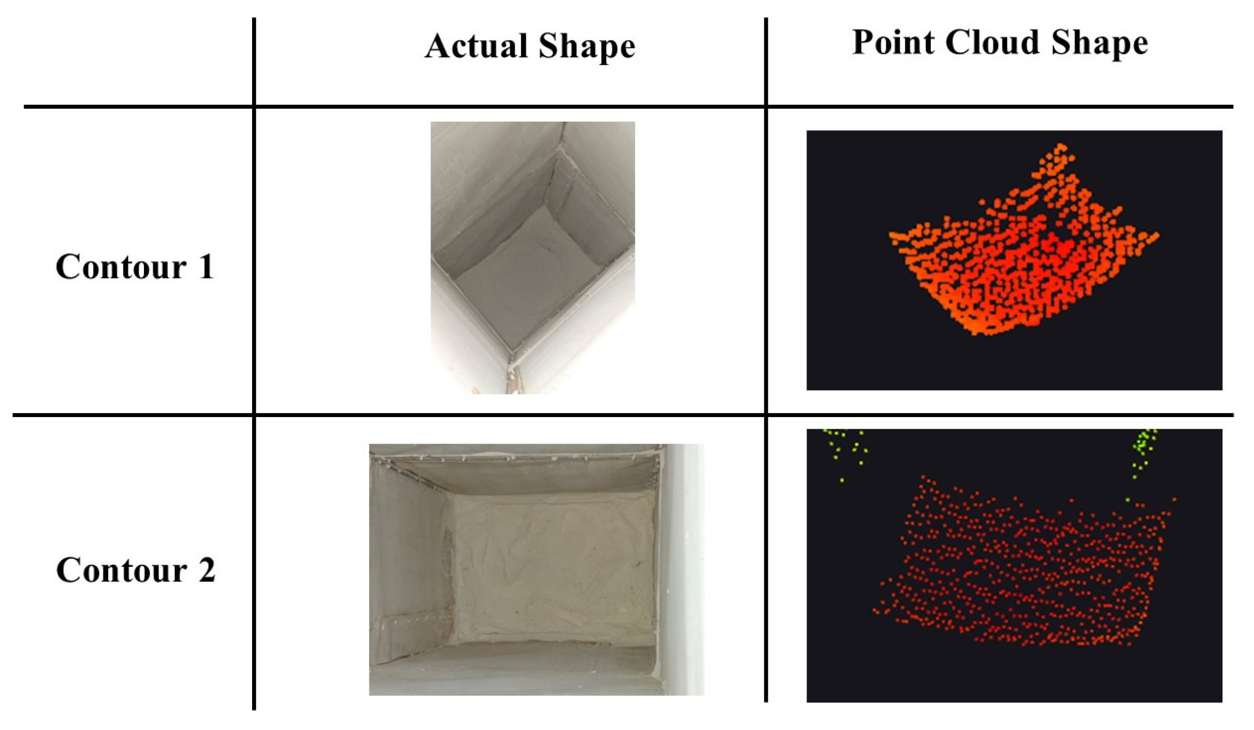
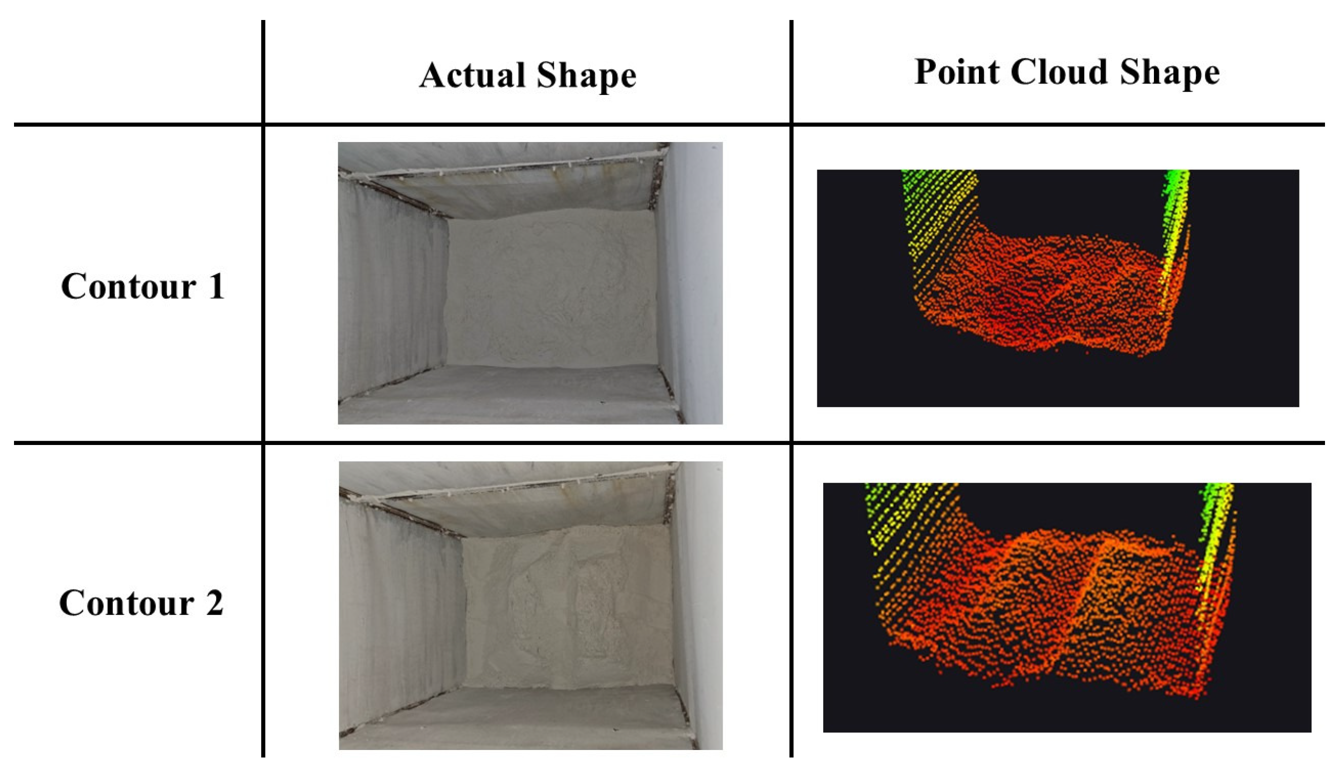
Figure 20 illustrates the actual flour surface contours along with the point cloud shapes generated by the system. Table 7 presents the calibration result of the volume measurement of the system, which compares the measured volumes of two contours against a known volume of 0.0594 m3 across five trials. Contour 1 exhibited an average measured volume of 0.059678 m3, resulting in a slightly higher estimation of the actual volume. On the other hand, Contour 2 demonstrated a closer correspondence with the known volume, with an average measurement of 0.0595 m3. Both contours displayed minimal deviations in measured volume across trials, suggesting reasonable accuracy and precision.

3.6.2. Storage Bin Filled with 0.4752 m3 of Flour

A flour volume of 0.4752 m3 was filled into the storage bin. Figure 21 illustrates the actual flour surface contours along with the scanned point cloud contour generated by the system. The measured volumes across the two contours and the distribution of the data are presented in Table 8. Table 8 presents the results of volume measurement calibration for the system across two contours, compared against a known volume of 0.4752 m3. Over five trials, Contour 1’s measured volumes range from 0.470279 m3 to 0.4805594 m3, with an average of 0.47407038 m3, a slightly lower estimation compared to the actual volume. Contour 2’s measurements range from 0.464461 m3 to 0.485587 m3, with an average of 0.473391 m3, also slightly underestimating the actual volume. Both contours show minor variations, with Contour 1 being marginally closer to the actual volume on average.

3.6.3. Storage Bin Filled with 0.7128 m3 of Flour

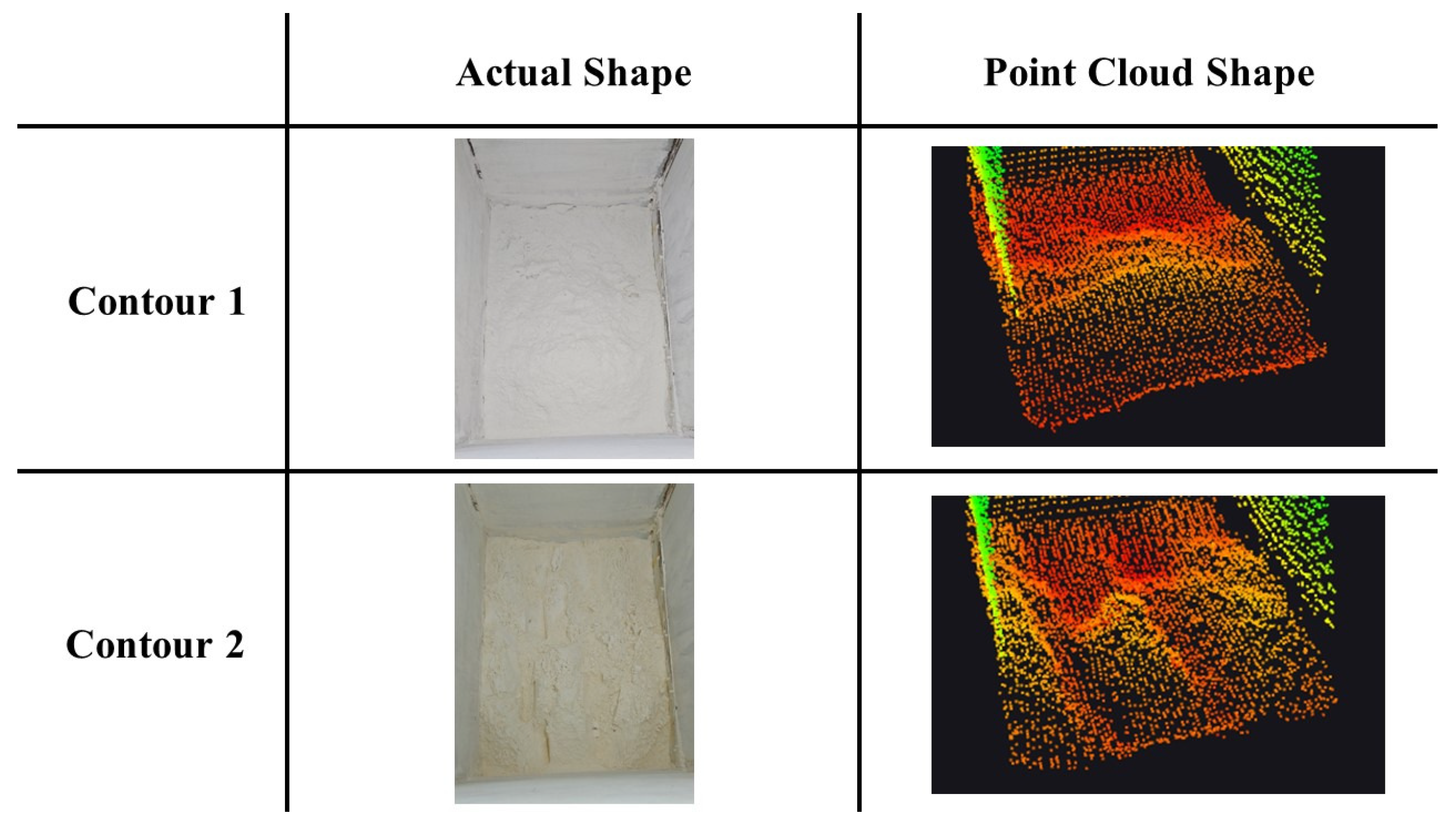
A volume of 0.7128 m3 was filled into the storage bin. Figure 22 illustrates the actual flour surface contours along with the scanned point cloud contour generated by the system. Table 9 presents the calibration results of the system’s volume measurements across two contours, compared against a known volume of 0.7128 m3, filled into the flour bin. Over five trials, Contour 1 achieved an average measured volume of 0.7178206 m3, slightly higher than the known volume. Contour 2 achieved an average measured volume of 0.7202706 m3, also slightly higher than the known volume. Both contours show minor variations, with Contour 1 being marginally closer to the known volume on average.
Table 9 presents the calibration results of volume measurements of the system across two contours, compared against a known volume of 0.7128 m3 filled in the flour bin.
The study conducted a statistical analysis using ANOVA for the three (3) different volume quantities filled into the storage bin. The results of the analysis are shown in Table 10, Table 11 and Table 12 below. Based on the conducted analysis, there was no statistical difference between the measurements based on the actual volume and those with different contours measured by the system, with a p-value greater than 0.05.

3.6.4. Volume Measurement Using the System and Sounding Method Result

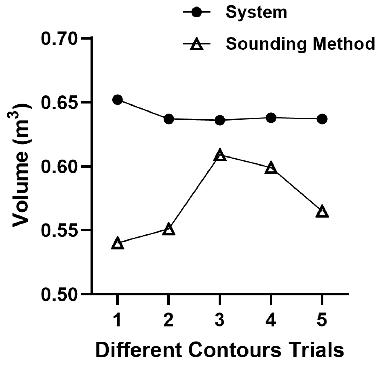
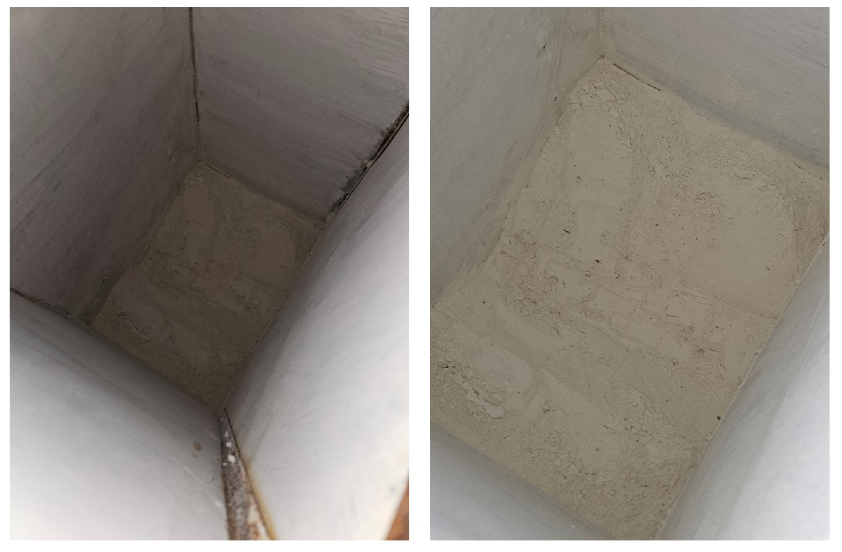
Table 13 presents the measured volumes using both methods for each contour shape and the percentage difference between them. The system measured an average cubic meter of 0.640, while the sounding method gathered 0.573 m3. The graph shown in Figure 23 represents the distribution of volumes obtained from two different methods (system and sounding) for five contour trials. The actual testing images and scanned point cloud of the system are depicted in Figure 23 and Figure 24.
Table 13 compares the volume measurements obtained using the 3D Point Cloud Scanner System and the traditional sounding method against an actual volume of 0.639 m3 across five trials, each with a different contour surface of flour. The system’s measurements ranged from 0.636 m3 to 0.642 m3, with an average of 0.640 m3, closely matching the actual volume. In contrast, the sounding method’s measurements ranged from 0.540 m3 to 0.609 m3, with an average of 0.573 m3, which is significantly lower than the actual volume. This comparison highlights that the 3D Point Cloud Scanner System provides measurements much closer to the actual volume than the traditional sounding method.
The comparison results demonstrate that the 3D Point Cloud Scanner System provides volume measurements that are consistent with those obtained using the traditional sounding method, regardless of the shape of the surface contour. The percentage differences between the two methods were minimal, indicating a high level of agreement. The statistical analysis conducted for the comparison in Table 13 suggests that since the p-value is less than 0.05, as shown in the statistical data in Table 14, there is strong evidence to suggest that there is a significant difference between the sample mean of the sounding method data and the population mean of the system data. In other words, the sounding method measurements are significantly different from the system volume measurements.

3.7. System Evaluation

The system evaluation section provides a comprehensive assessment of the 3D Point Cloud Scanner System’s performance based on the data obtained from various testing procedures. This includes the evaluation of LiDAR calibration, servo calibration, empty storage volume measurement, different volume quantity measurements, and comparison of the system and sounding method.

3.7.1. LiDAR Calibration Evaluation

Evaluation of the LiDAR device and servo calibration revealed consistent performance across different ranges. The highest Mean Absolute Error (MAE) of 0.0351 m was observed at a distance of 3 m, while the lowest MAE of 0.01616 m was recorded at 1.5 m. Additionally, the average Standard Deviation of 0.0103 m across the five different distances signifies consistent precision in measurements. These results demonstrate the accurate and precise performance of the LiDAR device in capturing range data across varying distances.

3.7.2. Servo Calibration Evaluation

Evaluation of the servo calibration revealed consistent performance at different angles. The highest Mean Absolute Error (MAE) was 0.6 degrees, while the lowest MAE was 0.2 degrees. These results indicate reliable performance in accurately positioning the servo motor, ensuring precise control over the scanning mechanism of the system.

3.7.3. Empty Storage Volume Measurement

The average measured volume in all trials was determined to be 1.00919 m3, with an uncertainty of 0.0155 m3. The gathered Mean Absolute Percentage Error (MAPE) was calculated to be 0.599377608%, indicating the system’s performance in accurately estimating the volume relative to the actual volume. Additionally, the standard deviation of the measured volumes was determined to be 0.007835601 m3, presenting the consistency and precision of the system’s volume measurements across multiple trials.

3.7.4. Different Volume Quantity Measurement

The system achieved an average MAPE of 1.01308% across all different volumes filled into the storage bin and an average standard deviation of 0.004691289 m3, across the three conducted tests. This indicates that the system shows a consistent level of accuracy in measuring the volume of flour across different quantities. The average MAPE value of 1.01308% suggests a minor deviation from the actual volume, which is within an acceptable range for the intended application. Additionally, the average standard deviation of 0.004691289 m3 reflects the precision and consistency of the system’s volume measurements. Overall, these results demonstrate the system’s capability to accurately and reliably measure the volume of flour across varying storage capacities, providing valuable insights for its practical implementation and use.

3.7.5. Comparison of the System and Sounding Method

These results validate the accuracy of the overall performance of the system and suggest that it is a reliable alternative to the traditional sounding method for measuring the volume of flour in storage bins. Additionally, statistical analysis indicates that with a p-value below 0.05, there is strong evidence to support that the sample mean of the sounding method data differs significantly from the population mean of the system data. In other words, the measurements obtained using the sounding method are notably different from those of the system volume. The system’s ability to provide consistent and accurate measurements across different surface contours, combined with its automation for estimation of the volume, offers significant advantages over manual methods, particularly in terms of efficiency and reduction of human error.

3.7.6. Limitation of Convex Hull Algorithm

While the convex hull algorithm can generate volumetric approximations for this study, it assumes the bounding geometry is convex. Because the actual physical surface of settled flour can exhibit non-convex topologies (as observed in certain regions of Figure 25), using convex hull introduces a minor geometric approximation error. In this prototype, the error was mitigated by calculating the volume of the empty space ( V e m p t y ) rather than the flour heap itself; under the tested filling scenarios, the inverted perspective of the empty-space boundaries behaved predominantly as a convex shape. This allowed the computationally lightweight algorithm to still achieve an acceptable 1.01% MAPE, though it lacks a universal guarantee for all possible flour distribution patterns.

4. Conclusions and Recommendations

The study successfully designed and developed a web-based 3D Point Cloud Scanner System to measure product volume inside a flour storage bin. The integration of the 3D scanner and web application achieved the study’s objectives. The testing showed that the system accurately measured the volume of flour materials in the storage bin. Statistical analysis confirmed that there was no significant difference between the measured volume of the system and the known volume of the bin. In addition, compared to traditional methods, the volume measurements of the system showed a significant improvement in accuracy. This improvement is further emphasized by statistical analysis, which revealed a notable difference between the sounding method data and the system data. These results suggest that the developed system is more accurate than manual or traditional methods, such as the sounding method, and has strong potential for applications in monitoring storage capacity.
While the proposed system presents high accuracy and cost-effectiveness under idle-state conditions, scaling this technology for continuous industrial deployment presents valuable avenues for future research. Currently, the system successfully mitigates signal degradation caused by dense airborne flour particulates, which can induce Mie scattering by employing a scheduled settling period prior to scanning. To apply dynamic volume tracking during active filling and emptying cycles, future iterations could integrate multi-echo LiDAR technology to better penetrate particulate clouds, paired with advanced point cloud filtering algorithms to isolate dust artifacts. Additionally, transitioning from a mechanically actuated sensor to emerging low-cost solid-state LiDARs would eliminate moving parts. As a result, it can reduce mechanical wear and maximize long-term durability in harsh environments. Because these advanced sensor and algorithmic upgrades will increase point cloud density, migrating from the current Raspberry Pi architecture to more advanced edge-computing platforms will be practical to maintain rapid processing efficiency. Furthermore, a software upgrade will involve transitioning from the current convex hull volume calculation to the classical Ball-Pivoting Algorithm (BPA) for surface reconstruction. Because the BPA does not rely on convexity assumptions, it will allow the system to map and calculate volumes for highly irregular, non-convex flour topographies. Lastly, implementing these enhancements alongside extensive field testing in larger-scale commercial silos will further bridge the gap between low-cost industrial-grade automation.

Author Contributions

Conceptualization, J.O., E.R.A., and C.J.S.; methodology, J.O., E.R.A. and C.J.S.; software, J.O., E.R.A., F.J.A. and C.J.S.; validation, J.O., E.R.A. and C.J.S.; formal analysis, J.O., E.R.A. and C.J.S.; investigation J.O., I.P., F.J.A. and C.J.S.; resources, J.O., I.P., F.J.A. and C.J.S.; data curation, J.O. and C.J.S.; writing—original paper draft preparation, J.P., M.M.M., R.C.II and C.J.S.; writing—review and editing, J.P., E.R.A., F.J.A., R.C.II and C.J.S. All authors have read and agreed to the published version of the manuscript.

Funding

This research received no external funding.

Data Availability Statement

The original contributions presented in this study are included in the article. Further inquiries can be directed to the corresponding authors.

Conflicts of Interest

The authors declare no conflicts of interest.

References

  1. Peters, D. Raw Materials. In White Biotechnology; Springer: Berlin/Heidelberg, Germany, 2007; pp. 1–30. [Google Scholar] [CrossRef] [Scilit]
  2. Rațu, R.N.; Veleșcu, I.D.; Stoica, F.; Usturoi, A.; Arsenoaia, V.N.; Crivei, I.C.; Postolache, A.N.; Lipșa, F.D.; Filipov, F.; Florea, A.M.; et al. Application of Agri-Food By-Products in the Food Industry. Agriculture 2023, 13, 1559. [Google Scholar] [CrossRef] [Scilit]
  3. Helkar, P.B.; Sahoo, A.; Patil, N. Review: Food Industry By-Products used as a Functional Food Ingredients. Int. J. Waste Resour. 2016, 6, 1–6. [Google Scholar]
  4. Bucklin, R.; Thompson, S.; Montross, M.; Abdel-Hadi, A. Chapter 9—Grain Storage Systems Design. In Handbook of Farm, Dairy and Food Machinery Engineering, 3rd ed.; Kutz, M., Ed.; Academic Press: Cambridge, MA, USA, 2019; pp. 175–223. [Google Scholar] [CrossRef] [Scilit]
  5. Yegorova, S.V.; Slavyanskiy, A.A.; Postnikova, T.A.; Pereboev, A.V.; Mazanova, G.V.; Murzakov, M.G. Improving the technology of post-harvest processing and storage of grain raw materials at the enterprises of the grain processing industry. IOP Conf. Ser. Earth Environ. Sci. 2021, 640, 022040. [Google Scholar] [CrossRef] [Scilit]
  6. Ding, W.; Zhang, K.; Shao, C. A fast volume measurement method for obtaining point cloud data from bulk stockpiles. Meas. Sci. Technol. 2023, 34, 105204. [Google Scholar] [CrossRef] [Scilit]
  7. Turner, A.; Jackson, J.; Koeninger, N.; Mcneill, S.; Montross, M.; Casada, M.; Boac, J.; Bhadra, R.; Maghirang, R.; Thompson, S. Error Analysis of Stored Grain Inventory Determination. Trans. ASABE 2016, 59, 1061–1072. [Google Scholar] [CrossRef] [Scilit]
  8. Bulut, S.; Giese, T.G.; Wende, M.; Anderl, R. The Paperless Factory: From Document Driven Factories to Model Driven Factories. In Proceedings of the 2020 IEEE International Conference on Teaching, Assessment, and Learning for Engineering (TALE), Takamatsu, Japan, 8–11 December 2020; pp. 725–730. [Google Scholar] [CrossRef] [Scilit]
  9. Williams, G.D.; Rosentrater, K.A. Design considerations for the construction and operation of flour milling facilities. Part I: Planning, structural, and life safety considerations. In Proceedings of the ASABE Annual International Meeting, Minneapolis, Minnesota, 17–20 June 2007; pp. 1–23. [Google Scholar] [CrossRef] [Scilit]
  10. Yu, X.; Liao, N.; Tao, C.; Zhang, X.; Zhou, B.; Zhang, H. Dust-concentration measurement based on Mie scattering of a laser beam. PLoS ONE 2017, 12, e0181575. [Google Scholar] [CrossRef] [Scilit] [PubMed]
  11. He, Q.; Nie, S.; Yin, S.; Cheng, Y.; Ma, F. Quantitative analysis and mitigation of dust interference in laser methane sensors: Impact on false alarms and measurement accuracy. Sens. Actuators A Phys. 2025, 384, 116753. [Google Scholar] [CrossRef] [Scilit]
  12. Ming, K.; Wang, C.; Xue, X.; Wu, J.; Chen, T. Parameter optimization for Rayleigh–Mie lidar under different dust conditions for the landing area of Martian Tianwen-1. Earth Planet. Phys. 2024, 8, 899–909. [Google Scholar] [CrossRef] [Scilit]
  13. Miranda-Fuentes, A.; Llorens, J.; Gamarra-Diezma, J.L.; Gil-Ribes, J.A.; Gil, E. Towards an Optimized Method of Olive Tree Crown Volume Measurement. Sensors 2015, 15, 3671–3687. [Google Scholar] [CrossRef] [Scilit] [PubMed]
  14. Turner, A.; Jackson, J.; Koeninger, N.; Mcneill, S.; Montross, M.; Casada, J.; Boac, R.; Bhadra, R.; Maghirang, S.; Thompson, S.A. Stored Grain Volume Measurement Using a Low Density Point Cloud. Appl. Eng. Agric. 2017, 33, 105–112. [Google Scholar] [CrossRef] [Scilit]
  15. Xu, J.; Lu, Y.; Olaniyi, E.; Harvey, L. Online volume measurement of sweetpotatoes by a LiDAR-based machine vision system. J. Food Eng. 2024, 361, 111725. [Google Scholar] [CrossRef] [Scilit]
  16. Wang, Y.; Weinacker, H.; Koch, B. A Lidar Point Cloud Based Procedure for Vertical Canopy Structure Analysis And 3D Single Tree Modelling in Forest. Sensors 2008, 8, 3938–3951. [Google Scholar] [CrossRef] [Scilit] [PubMed]
  17. Wang, Q.; Kim, M.K. Applications of 3D point cloud data in the construction industry: A fifteen-year review from 2004 to 2018. Adv. Eng. Inform. 2019, 39, 306–319. [Google Scholar] [CrossRef] [Scilit]
  18. Jochem, A.; Hollaus, M.; Rutzinger, M.; Höfle, B. Estimation of Aboveground Biomass in Alpine Forests: A Semi-Empirical Approach Considering Canopy Transparency Derived from Airborne LiDAR Data. Sensors 2011, 11, 278–295. [Google Scholar] [CrossRef] [Scilit] [PubMed]
  19. Denysyuk, P.; Teslyuk, V.; Chorna, I. Development of mobile robot using LIDAR technology based on Arduino controller. In Proceedings of the 2018 XIVth International Conference on Perspective Technologies and Methods in MEMS Design (MEMSTECH), Lviv, Ukraine, 18–22 April 2018; pp. 240–244. [Google Scholar] [CrossRef] [Scilit]
  20. Cai, H.; Ye, Z.; Yao, F.; Lv, C.; Cheng, X.; Xiang, L. Streak Tube-Based LiDAR for 3D Imaging. Sensors 2025, 25, 5348. [Google Scholar] [CrossRef] [Scilit] [PubMed]
  21. Fortuna, S.; Chiodini, S.; Valmorbida, A.; Pertile, M. Comparative Analysis of LiDAR-SLAM Systems: A Study of a Motorized Optomechanical LiDAR and an MEMS Scanner LiDAR. Sensors 2025, 25, 5352. [Google Scholar] [CrossRef] [Scilit] [PubMed]
  22. Lv, D.; Ying, X.; Cui, Y.; Song, J.; Qian, K.; Li, M. Research on the technology of LIDAR data processing. In Proceedings of the 2017 First International Conference on Electronics Instrumentation & Information Systems (EIIS), Harbin, China, 3–5 June 2017; pp. 1–5. [Google Scholar] [CrossRef] [Scilit]
  23. Llop, J.; Gil, E.; Llorens, J.; Miranda-Fuentes, A.; Gallart, M. Testing the Suitability of a Terrestrial 2D LiDAR Scanner for Canopy Characterization of Greenhouse Tomato Crops. Sensors 2016, 16, 1435. [Google Scholar] [CrossRef] [Scilit] [PubMed]
  24. Zhao, L.; Gao, Y. A LiDAR-Inertial Odometry Method, System, Device, and Medium. CN117685999A, 12 March 2024. [Google Scholar]
  25. Clar, S.E.; Aleluya, E.R.M.; Salaan, C.J.O. Volume Estimation of Raw Materials inside the Silo using Convex Hull Method. In Proceedings of the 2022 IEEE 14th International Conference on Humanoid, Nanotechnology, Information Technology, Communication and Control, Environment, and Management (HNICEM), Boracay Island, Philippines, 1–4 December 2022; pp. 1–6. [Google Scholar] [CrossRef] [Scilit]
  26. Tan, J.; Pan, G.; Karafin, J.; Nonn, T.; Hernandez Zaragoza, J.C. Combining Light-Field Data with Active Depth Data for Depth Map Generation. U.S. Patent 11328446B2, 10 May 2022. [Google Scholar]
  27. Theverapperuma, L.; Halder, B.; Balasubramanian, K. Techniques for Volume Estimation. JP2025003969A, 14 January 2025. [Google Scholar]
  28. Jeong, S.; Jeon, Y.; An, S.; Kim, Y.; Choi, E. Point Cloud-Based Method and Apparatus for Estimating the Volume of Stacked Objects. KR20230099545A, 4 July 2023. [Google Scholar]
  29. Lei, J.; Liu, R.; Mei, S.; Luo, H.; Yang, X.; Luo, Y.; Li, W.; Wei, W. Large Irregular Stacking Volume Real-Time Measurement Method Based on Binocular Stereo Matching. CN118134994A, 4 June 2024. [Google Scholar]
  30. Barzilay, O.; Abramson, J. Estimation of 3D Point Candidates from a Location in a Single Image. U.S. Patent 10593054B2, 17 March 2020. [Google Scholar]
  31. Bernardini, F.; Mittleman, J.; Rushmeier, H.; Silva, C.; Taubin, G. The ball-pivoting algorithm for surface reconstruction. IEEE Trans. Vis. Comput. Graph. 1999, 5, 349–359. [Google Scholar] [CrossRef] [Scilit]
  32. Anoop, S.; Abhishek, R.; Siddeswara Prasad, V. Volume Measurement For Silos. In Proceedings of the IEEE International Conference on Electronics, Computing and Communication Technologies (CONECCT), Bangalore, India, 9–11 July 2021; pp. 1–5. [Google Scholar] [CrossRef] [Scilit]
  33. Manish, R.; Hasheminasab, S.M.; Liu, J.; Koshan, Y.; Mahlberg, J.A.; Lin, Y.; Ravi, R.; Zhou, T.; McGuffey, J.; Wells, T.; et al. Image-Aided LiDAR Mapping Platform and Data Processing Strategy for Stockpile Volume Estimation. Remote Sens. 2022, 14, 231. [Google Scholar] [CrossRef] [Scilit]
  34. Chua, C.K.; Wong, C.H.; Yeong, W.Y. Chapter Four—Software and Data Format. In Standards, Quality Control, and Measurement Sciences in 3D Printing and Additive Manufacturing; Chua, C.K., Wong, C.H., Yeong, W.Y., Eds.; Academic Press: Cambridge, MA, USA, 2017; pp. 75–94. [Google Scholar] [CrossRef] [Scilit]
  35. Bi, S.; Yuan, C.; Liu, C.; Cheng, J.; Wang, W.; Cai, Y. A Survey of Low-Cost 3D Laser Scanning Technology. Appl. Sci. 2021, 11, 3938. [Google Scholar] [CrossRef] [Scilit]
  36. Barber, C.B.; Dobkin, D.P.; Huhdanpaa, H.T. The Quickhull algorithm for convex hulls. ACM Trans. Math. Softw. (TOMS) 1996, 22, 469–483. [Google Scholar] [CrossRef] [Scilit]
  37. Siebers, M.H.; Fu, P.; Blakely, B.J.; Long, S.P.; Bernacchi, C.J.; McGrath, J.M. Fast, Nondestructive and Precise Biomass Measurements Are Possible Using Lidar-Based Convex Hull and Voxelization Algorithms. Remote Sens. 2024, 16, 2191. [Google Scholar] [CrossRef] [Scilit]
  38. Raba, D.; Gurt, S.; Vila, O.; Farres, E. An Internet of Things (IoT) solution to optimise the livestock feed supply chain. Comput. Sci. Inf. Technol. 2020, 10, 103–118. [Google Scholar] [CrossRef] [Scilit]
Figure 1. Comparison of sensing coverage geometries for volumetric measurement in enclosed flour bins: (a) typical coverage of a commercially available 3D LiDAR, characterized by fixed vertical beam angles and limited downward field of view; (b) proposed rotating 2D LiDAR configuration, in which a dense planar scan is incrementally swept across predefined elevation angles to achieve controlled downward hemispherical coverage of the bin interior.
Technologies 14 00401 g001
Figure 2. Conceptual comparison of sensing coverage in an enclosed flour storage bin: (a) a typical commercial 3D LiDAR provides limited downward coverage due to fixed beam elevation angles which results in blind regions over the granular material surface; (b) the proposed rotating 2D LiDAR actively sweeps a dense planar scan across elevation that attains controlled downward hemispherical coverage and complete observation of the bin interior surface.
Technologies 14 00401 g002
Figure 3. General conceptual flow of the 3D point cloud scanning, processing, and evaluation system. The process is divided into three stages: development of the scanner and mock-up, point cloud data processing, and testing with validation.
Technologies 14 00401 g003
Figure 4. System architecture for: (A) 3D Point Cloud Scanner System; (B) web application.
Technologies 14 00401 g004
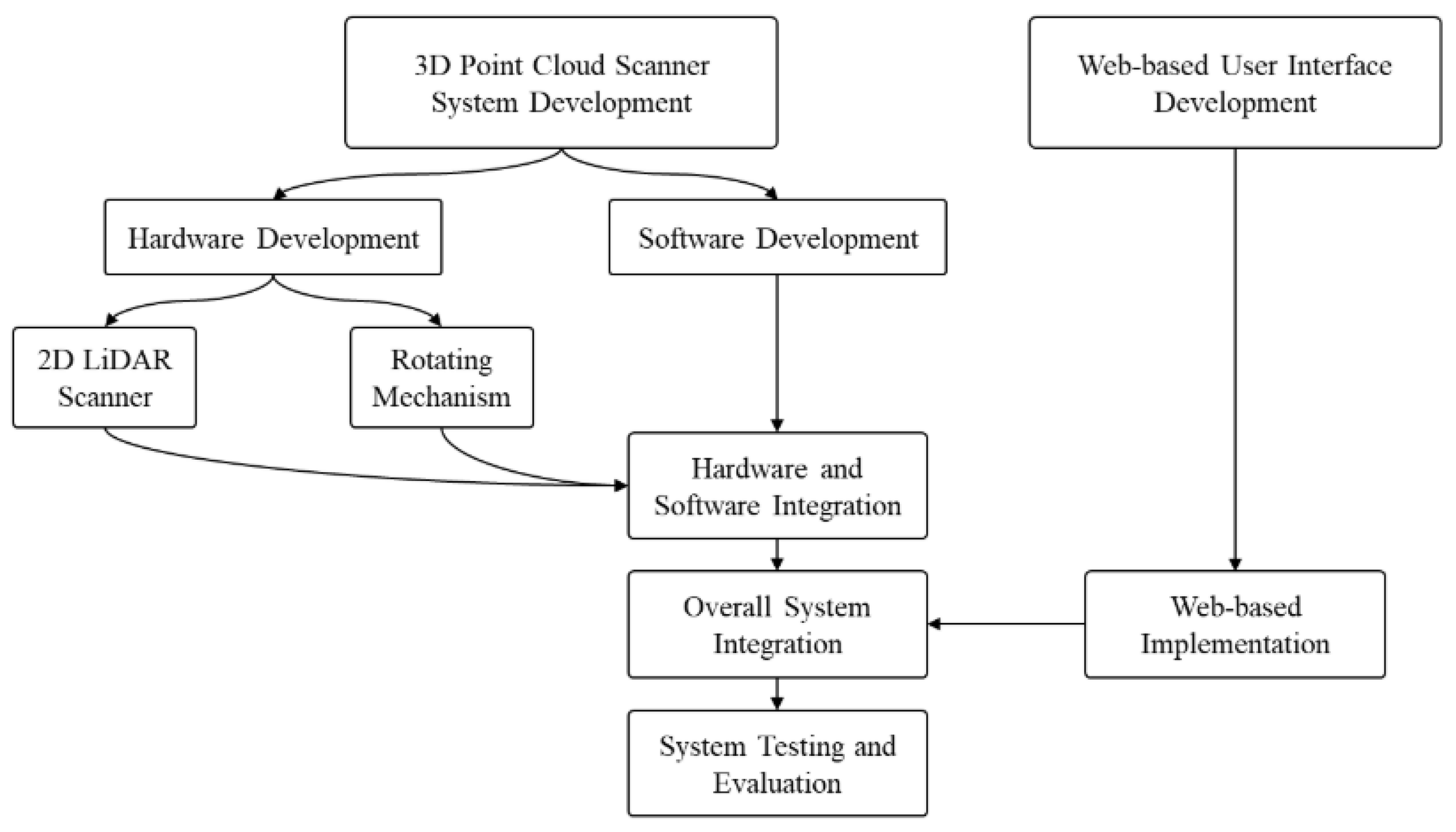
Figure 5. System development process that starts with hardware and software development, including a 2D LiDAR scanner and rotating mechanism. These are integrated through hardware–software integration, followed by overall system integration with the web application. The final stage involves system testing and evaluation to ensure performance and reliability.
Technologies 14 00401 g005
Figure 6. Scan direction of LiDAR and movement direction of the servo. The top view shows the 2D LiDAR scanning from 0° to 180°, while the servo motor controls rotation. The side views illustrate the servo’s movement along the z-axis, enabling full coverage of the scanning area.
Technologies 14 00401 g006
Figure 7. Different views of the CAD model design of the 3D Point Cloud Scanner System. The side view highlights the servo motor, the bottom view shows the 2D LiDAR device, and the isometric view presents the full system with its compartment.
Technologies 14 00401 g007
Figure 8. Specific components of the system. The setup consists of a YDLiDAR X4 sensor, Raspberry Pi 4 Model B for control, and an AX-12A actuator. Power is supplied by a 22.2 V battery regulated through step-down converters to provide 5 V and 11.2 V outputs for the components.
Technologies 14 00401 g008
Figure 9. Overall circuit diagram. The system uses a 22.2 V battery regulated by two buck converters to supply 11.2 V for the AX–12A Dynamixel and 5 V for the Raspberry Pi 4 Model B and YDLiDAR X4. Green, red and black lines represent data, power and ground connections, respectively.
Technologies 14 00401 g009
Figure 10. ROS node architecture showing publish–subscribe structure. The remote command node coordinates scanning by communicating with the LiDAR and Dynamixel servo nodes, which publish scan and position topics. The scan-to-3D-point-cloud-mapping node and post-processing node handle data conversion and refinement. Processed point clouds and measured volumes are then shared with the web application through the Rosbridge server node.
Technologies 14 00401 g010
Figure 11. Main dashboard of the web-based interface showing system status, point cloud visualization, and volume metrics.
Technologies 14 00401 g011
Figure 12. CAD model design of the storage bin.
Technologies 14 00401 g012
Figure 13. Actual 3D Point Cloud Scanner System developed and its components.
Technologies 14 00401 g013
Figure 14. Example of the volume estimation process of the system. Raw LiDAR data is converted into a 3D point cloud, meshed using the Quickhull algorithm, and processed to estimate volume, yielding 1.0129 m3. In the 3D point cloud visualization, color indicates distance from the LiDAR sensor: red points at the bottom of the silo represent the farthest areas, while blue points indicate the closest.
Technologies 14 00401 g014
Figure 15. Actual flour storage bin created. The constructed bin consists of three main sections: a rectangular upper body, a pyramidal frustum transition, and a conical frustum at the bottom for directing the stored material.
Technologies 14 00401 g015
Figure 16. Testing field and actual system setup. The figure shows the deployment of the 3D scanner system at the flour storage bin site, including modem connection, scanner placement inside the bin, and the web application interface for real-time monitoring and volume measurement.
Technologies 14 00401 g016
Figure 17. Actual empty bin and scanned point cloud data. The left image shows the physical empty storage bin, while the right images present its corresponding 3D point cloud shape generated from LiDAR scanning. In the 3D point cloud data, the red points at the bottom of the silo represent the farthest distances from the LiDAR, while colors in the blue spectrum indicate the nearest points.
Technologies 14 00401 g017
Figure 18. Actual web visualization of point cloud and volume.
Technologies 14 00401 g018
Figure 19. Container with a known volume used for testing. The container was utilized as a reference object to validate the accuracy of the system’s volume estimation.
Technologies 14 00401 g019
Figure 20. Comparison of actual and point cloud surface contours for Test 1. The left column shows the physical container for two different contours, while the right column presents the corresponding point cloud surfaces generated by the system. The nearly uniform color across the point cloud surface indicates that the material is almost completely flat and possesses no convexity.
Technologies 14 00401 g020
Figure 21. Actual and generated point cloud surface contours for Test 2. As shown in the point cloud representation, the varying color intensities illustrate the convexity of the material which depicts the unevenness of the surface.
Technologies 14 00401 g021
Figure 22. Comparison of actual and point cloud surface contours for Test 3. The changing color intensities on the generated point cloud surface depict varying degrees of convexity.
Technologies 14 00401 g022
Figure 23. Distribution of volume measurements obtained from the system and sounding method. The graph compares system-estimated volumes with traditional sounding across five contour trials, showing the system’s consistency and reduced variability.
Technologies 14 00401 g023
Figure 24. Actual testing setup of Contour 1 using system and sounding method. The images show the physical contour setup inside the bin, where both the developed system and the traditional sounding method were applied for volume measurement.
Technologies 14 00401 g024
Figure 25. 3D point cloud surface of Contour 1. The visualization displays the scanned volume profile generated by the system, which is used for comparison against the manual sounding method. In this representation, color indicates distance from the LiDAR sensor: red points at the bottom of the silo represent the farthest areas, while blue points indicate the closest.
Technologies 14 00401 g025
Table 1. Comparison of sensor, processing, and deployment characteristics of bulk material volume estimation systems.
CriteriaSurface Reconstruction [31]Volume Measurement for Silos [32]Stockpile Volume Estimation [33]Proposed System
Sensor typeNot applicable2D LiDARLiDAR and Camera2D LiDAR with controlled rotation
Scanning geometryNot applicableAutomated pan–tilt (360°, 180° tilt)Free-form scanning in open environmentsHalf-spherical scan optimized for silo geometry
Target environmentGeneral surfacesGrain silosOpen stockpilesEnclosed flour storage bins
Suitability for vertical storage binsNot applicableModerateLimited (open-space assumption)High
Data processing frameworkSurface mesh reconstructionPython (DBSCAN, convex hull integration)LiDAR–image fusion and post-processingROS pipeline with PCL-based processing
Point cloud handlingDense point setsLocal file-based storageDense 3D point cloudsPCL-based management with Three.js visualization
Surface reconstruction approachBall-Pivoting AlgorithmSlice-based convex hull integrationSurface reconstruction from fused dataConcavity-aware convex hull with partial correction
Granular surface concavity handlingPoor for irregular granular surfacesNot addressedLimitedExplicit concavity correction for granular materials
Container geometry constraintsNot addressedNot addressedNot addressedSilo geometry-aware convex hull constrained within bin boundaries
Volume computation methodNot applicableSlice-based numerical integrationMesh-based volume estimation3D surface reconstruction with volumetric integration
Remote scanning/operationNoNoNoYes (web-based monitoring interface)
Industrial deployabilityResearch-orientedModerateModerate (outdoor-focused)High (cost-efficient and geometry-
adaptive)
Primary applicationGeneral surface reconstructionGrain volume estimationStockpile volume estimationFlour bin volumetric measurement
Key ContributionGeneric surface reconstruction algorithmPlatform for stockpile volume estimationAutomated LiDAR-based grain volume estimationVolumetric measurement system for enclosed flour bins using 2D LiDAR with tilting mechanism or half-sphere FOV
Table 2. Practical limitations of commercially available 3D LiDAR products in achieving downward hemispherical coverage for enclosed flour bin volume measurement.
CriteriaVelodyne VLP-16RoboSense RS-LiDAR-16Ouster OS1Hesai PandarQTProposed System
LiDAR type3D multi-beam LiDAR3D multi-beam LiDAR3D multi-beam LiDAR3D multi-beam LiDAR2D LiDAR with tilting mechanism
Horizontal FOV360°360°360°360°270°–360° (mount-dependent)
Vertical FOV (fixed beam elevation range)30° (±15°)30° (±15°)45° (±22.5°)∼104° (≈−52° to +52°)∼180° effective (downward hemispherical)
Can achieve half-sphere coverage from a fixed mounting positionNoNoNoNoYes
Flour bulk surface visibility inside binPartial (large blind regions)Partial (large blind regions)Partial (large blind regions)Improved but still incompleteComprehensive surface coverage
Need for additional mechanical motion to extend vertical coverageYes (external)Yes (external)Yes (external)Yes (external)Integrated tilting mechanism
Designed for confined bin geometryNo (automotive/robotics)No (autonomous systems)No (robotics/mapping)No (ADAS/robotics)Yes (flour bin specific)
Material-specific optimizationGeneral-purposeGeneral-purposeGeneral-purposeGeneral-purposeFine granular material (flour)
System hardware cost> $ 4000 > $ 1500 > $ 4000 > $ 5000 < $ 300
Primary application domainAutonomous vehiclesAutonomous drivingRobotics & mappingADAS & roboticsFlour bin volume measurement
Note: Horizontal FOV is included to illustrate that commercial 3D LiDARs prioritize omnidirectional perception rather than downward volumetric coverage.
Table 3. LiDAR range calibration results.
Actual
Range (m)
Trial 1Trial 2Trial 3Trial 4Trial 5Average (m)SD
1.01.01341.01351.03671.01541.01351.01850.0099
1.51.52671.52781.51651.50731.49751.51520.0119
2.02.02892.03532.01452.01842.00952.02130.0101
2.52.52412.53422.50922.52762.55022.52910.0155
3.03.04123.03533.04523.02213.03173.03510.0087
Table 4. Servo angle calibration results.
Actual
Angle (°)
Trial 1Trial 2Trial 3Trial 4Trial 5Average (°)
35353635353535.2
70707170706970.0
105106105106104105105.2
140140141139141140140.2
175175175174174176174.8
Table 5. Individual and total volume of the storage bin.
ShapeTotal Volume (m3)
Rectangular0.9573
Pyramidal Frustum0.0077
Conical Frustum0.0478
Flour Bin Total Volume1.0129
Table 6. One-Sample t-test for actual and measured volumes of empty storage bin measurement result.
EstimateStatisticp ValueParameterConf. LowConf. HighMethodAlternative
1.013−0.3900.69936.0001.0121.013One Sample-testTwo Sided
Table 7. Volume measurement calibration result of the system across two contours with a known volume of 0.0594 m3.
TrialsMeasured Volume (m3)Known Volume (m3)
Contour 1Contour 2
10.060.05920.0594
20.059340.06010.0594
30.0589430.05890.0594
40.059760.05910.0594
50.0596780.06020.0594
Average0.0596780.0595
Table 8. Volume measurement calibration result of the system across two contours with a known volume of 0.4752 m3.
TrialsMeasured Volume (m3)Known Volume (m3)
Contour 1Contour 2
10.4704180.4729140.4752
20.4702790.4644610.4752
30.4720610.4737820.4752
40.48055940.4855870.4752
50.47703450.4702110.4752
Average0.474070380.473391
Table 9. Volume measurement calibration result of the system across two contours with a known volume of 0.7128 m3.
TrialsMeasured Volume (m3)Known Volume (m3)
Contour 1Contour 2
10.7163270.7258030.7128
20.7060010.7248730.7128
30.7202510.7294040.7128
40.716870.7158440.7128
50.7296540.7054290.7128
Average0.71782060.7202706
Table 10. ANOVA results of volume measurement calibration result of the system across two contours with a known volume of 0.0594 m3.
DfSum SqMean SqF ValuePr (F)
Variable2.00000.00000.00003.10890.0817
Residuals12.00000.00000.0000
Table 11. ANOVA results of volume measurement calibration result of the system across two contours with a known volume of 0.4752 m3.
DfSum Sq Mean Sq Statisticp. Value
Variable2.00000.00000.00001.20420.3337
Residuals12.00000.00000.0000
Table 12. ANOVA results of volume measurement calibration result of the system across two contours with a known volume of 0.7128 m3.
DfSum SqMean SqStatisticp. Value
Variable2.00000.00010.00004.02330.07323
Residuals12.00000.00000.0000
Table 13. Comparison of volume measurement using the 3D Point Cloud Scanner System and traditional sounding method for different surface contours.
TrialsMeasured Volume (m3)Actual Volume (m3)
SystemSounding Method
10.6420.5400.639
20.6370.5510.639
30.6360.6090.639
40.6380.5990.639
50.6370.5650.639
Average0.6400.573
Table 14. One-Sample test for comparison of volume measurement of the system vs. sounding method.
EstimateStatisticp ValueParameterConf. LowConf. HighMethodAlternative
0.573−5.0030.00750.5360.610One Sample-testTwo Sided
Disclaimer/Publisher’s Note: The statements, opinions and data contained in all publications are solely those of the individual author(s) and contributor(s) and not of MDPI and/or the editor(s). MDPI and/or the editor(s) disclaim responsibility for any injury to people or property resulting from any ideas, methods, instructions or products referred to in the content.