PI-Based Adaptive Actor–Critic Displacement Volume Control of Axial-Piston Pump

Abstract

This article presents the synthesis, implementation, and experimental study of a PI-based adaptive actor–critic displacement volume controller of an axial-piston pump intended for open-loop circuit hydraulic drive systems. The proposed control structure combines a conventional PI actor with an adaptive critic that estimates the infinite-horizon cost through Bellman-error minimization. By using the tracking error and its integral as actor inputs, the controller avoids the need for an accurate plant model while retaining a compact and practically implementable structure. The adaptive laws are derived using gradient-based learning, and a Lyapunov-based analysis establishes closed-loop stability for sufficiently small adaptation gains. The controller is implemented in a fixed-step Simulink^® environment and deployed on a rapid prototyping platform with real-time communication to an industrial microcontroller and proportional valve amplifier. The experimental results obtained under four fixed loading conditions and dynamic load variations demonstrate a stable operation, bounded critic behavior, and a near-zero Bellman error during learning. Comparative tests against a classical PI controller, a Lyapunov-based model reference adaptive controller, and a generic actor–critic scheme show that the proposed PI-based actor–critic achieves the lowest performance index and the shortest settling times in most cases.

1. Introduction

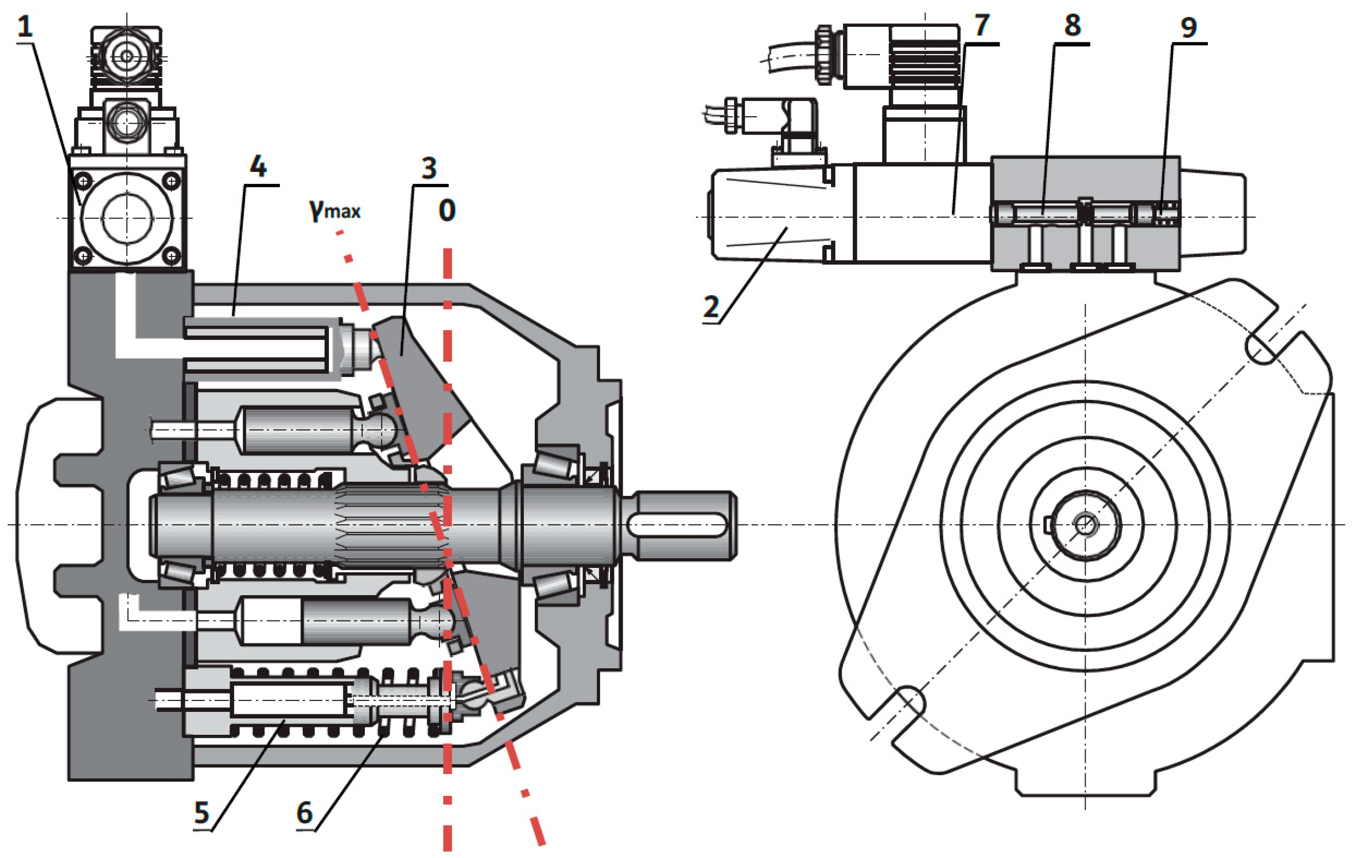
Axial-piston hydraulic machines are one of the most widely used in the practice of hydraulic drives. They exist both as working hydraulic machines (pumps) and as power hydraulic machines (motors). This type of hydraulic motor is characterized by high-speed operation while realizing high torque. According to the design features, axial-piston machines are of two main types: swash plate and bent axis. Both types have designs for open and closed circulation (e.g., hydrostatic transmissions) [1,2]. The main advantages considered in the aspect of axial-piston pumps are expressed in the high density of transmitted power (so-called power per unit weight), operation at high speeds (up to 4500 min⁻¹) and high pressure (which can reach up to 45 MPa), which is the reason for their compactness, smaller internal leakage (which is the reason for a high overall efficiency), and low level of generated noise (regardless of whether they are submerged or mounted outside the tank). The main advantages also include the possibility of regulating the displacement volume [3]. All of these advantages make axial-piston pumps preferred in systems with the volumetric speed regulation of hydraulic cylinders or motors. Of course, one main disadvantage should be noted—their cost is significantly higher than that of other types of hydraulic displacement machines, especially when they involve variable displacement.

There is a large set of regulators, especially for axial-piston pumps. Most often, regulators are hydro-mechanical and change the displacement volume of the pump according to a certain control law (pressure, flow rate, or power). Proportional to the change in the displacement volume of the pump, the flow rate supplied to the hydraulic system changes [4]. This makes pumps more studied than hydraulic motors, since they are the main source of hydraulic energy in drive systems.

With the development of hydraulic control devices with proportional electrical control, the possibilities for regulating the displacement volume of hydraulic pumps, especially the axial-piston type, are increasing [5]. The increase in possibilities is expressed in replacing the conventional hydro-mechanical regulator with an electrohydraulic proportional spool valve [5]. The valve has a significantly higher natural frequency and allows for the implementation of various control algorithms. Moreover, with the development of microcontrollers, it is possible for the control algorithm to be embedded (through a suitable programming language) or to work in real-time mode. The classic analogue electronic amplifier of the proportional valve is replaced by a digital microcontroller, for example, a PLC. This leads to additional possibilities, which are expressed in the fact that the classic PID controller [6] can be replaced with a significantly more complex but high control performance, advanced algorithm like LQG, H_∞, or μ [7,8,9,10,11,12,13,14,15,16,17,18,19]. The development of hydraulic drives with load-sensing has increased the application of adaptive algorithms [20,21,22,23,24,25,26,27]. All of these algorithms can be easily implemented in the microcontroller. That is, the difficulties are in the synthesis of such an advanced controller [28,29], as it requires an appropriate mathematical model that sufficiently accurately describes the dynamics of the plant, but the order of the dynamic components should not be particularly high. Deriving such a model using an analytical approach is often a difficult task, since there is no a priori information about the plant. In this case, it is more expedient to use the methods of system identification [30,31]. This makes it possible to obtain a suitable model based on an experimentally measured data set. Modern control theory also offers another approach to controller synthesis called the “model-free” approach. These approaches apply to an adaptive controller of the actor–critic type. It is a hybrid technique combining an actor (an adaptive controller that generates a control signal) and a critic (part of the controller that evaluates the performance index using a neural network), to control an uncertain nonlinear system in real time. Several publications exploited this technique to control different fluid power systems [32,33,34,35,36,37,38,39,40,41,42,43,44,45,46,47,48,49,50]. The authors have developed such a controller, which has been experimentally tested on a variable-displacement axial-piston pump designed for hydraulic systems with open circulation [51]. Despite the high control performance, the controller is complex to implement and is sensitive to the initial conditions. To start the system with the actor–critic controller in [51], the 12 initial values for the parameters, learning rate, and forgetting factor of the critic network must be chosen, and 10 values for the parameters, learning rate, and forgetting factor of the actor network must be set. The experiments with the laboratory setup show that the control system is more sensitive to the initial values of the actor network. This motivates the authors to simplify the structure of the adaptive controller, especially the actor part, in order to reduce the number of initial conditions. This is done by introducing an adaptive PI controller instead of a neural network that serves as an actor. In this way, the actor has only two parameters—proportional gain and integral gain. This creates the possibility for the easier selection of the appropriate initial conditions; for example, the system can start with some conservative values of adaptive PI controller parameters.

This type of controller has the following advantages:

• Prior information about the plant model is not required;
• There is great flexibility in choosing the critic parameters and structure;
• The critic is represented by a neural network that does not explicitly depend on the plant model;
• Optimal control in the sense of a defined cost function can be obtained;
• Stability for the learning rates lower than their upper limits is guaranteed;
• Analytical stability proof is possible.

However, some disadvantages of this type of controller are as follows:

• It is a complex algorithm for implementation, but simpler than the classical actor–critic model;
• It requires a compromise between the control performance and adaptation rate;
• There is a dependence on the initial parameter values.

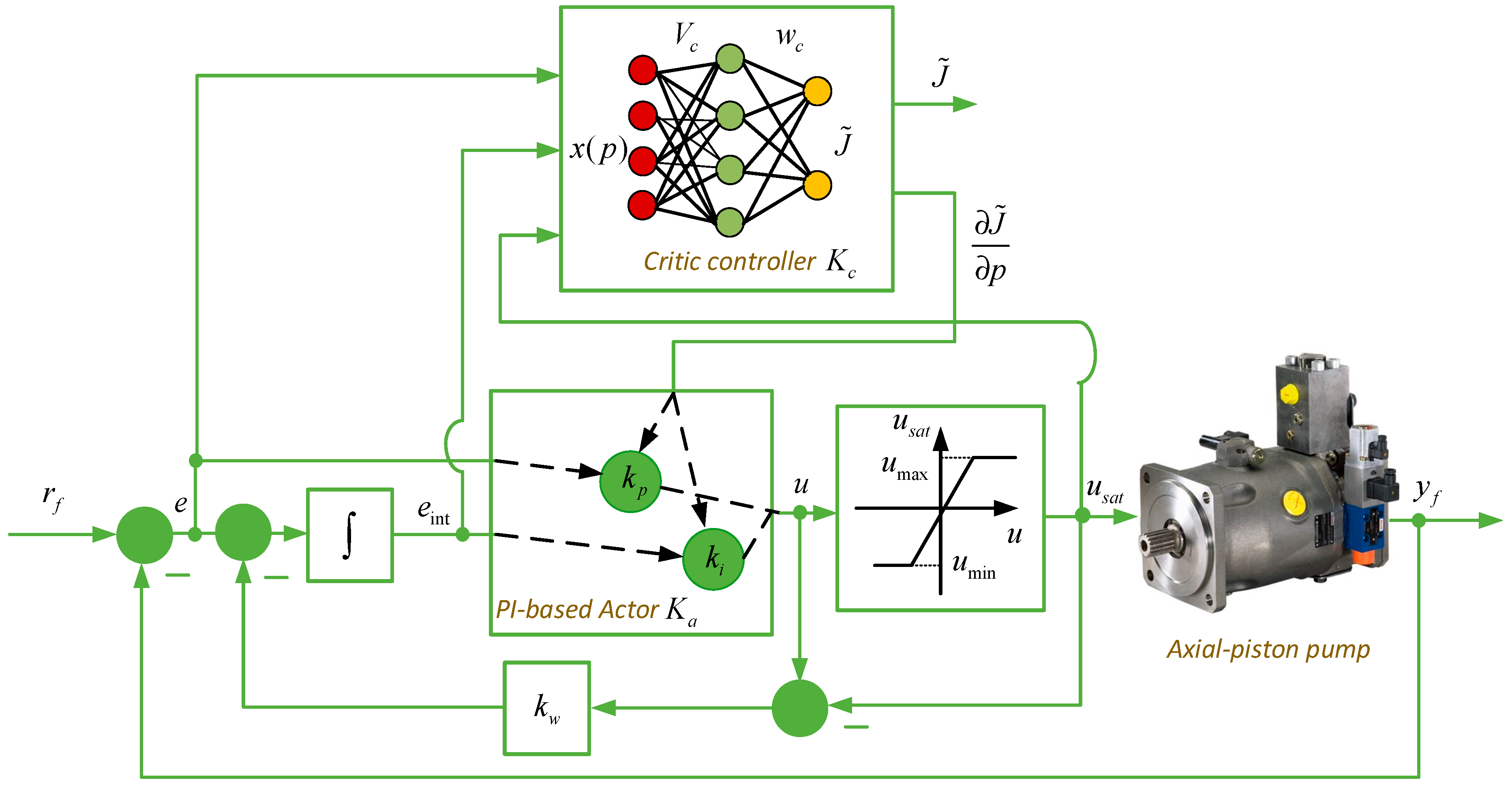
This article aims to present the design, implementation, and experimental evaluation of a PI-based adaptive actor–critic (PIAC) displacement volume controller of an axial-piston pump intended for open-loop circuit hydraulic drive systems. The design of the PIAC controller is based on an adaptive PI controller as the actor and a two-layer neural network as the critic. The activation functions are chosen as the tangent hyperbolic (tanh). The weights of the network are tuned in real time through the gradient descent algorithm. The criteria for tuning the PI-based actor are evaluated from the critic network via an approximation of the quadratic total cost to go. The critic network uses the recursive Bellman equation to calculate a Bellman error that is utilized for neural network parameter training.

The main article contributions are as follows:

• A new PI-based adaptive actor–critic control structure for axial-piston pump displacement volume control, using the tracking error and its integral as actor inputs, with online parameter adaptation via gradient backpropagation and gradient descent.
• A model-free design that avoids requiring an accurate plant model, making the controller easier to apply to uncertain hydraulic systems.
• Theoretical Lyapunov-based stability analysis showing that the closed-loop system remains asymptotically stable for sufficiently small learning rates, and that the adaptation speed trades off against stability.
• A real-time experimental implementation on a laboratory hydraulic test setup with a proportional valve, flow meter, pressure sensor, and MATLAB/Simulink® ver.2023a-based control hardware.
• A performance comparison against PI, Lyapunov-based model reference adaptive controller (LMRAC), and generalized actor–critic baselines (AC), showing better tracking performance and faster settling across multiple loading conditions and load variations.
• Evidence that the method achieves bounded critic signals and a near-zero Bellman error, supporting the convergence of the adaptive policy in the presence of hydraulic nonlinearities.

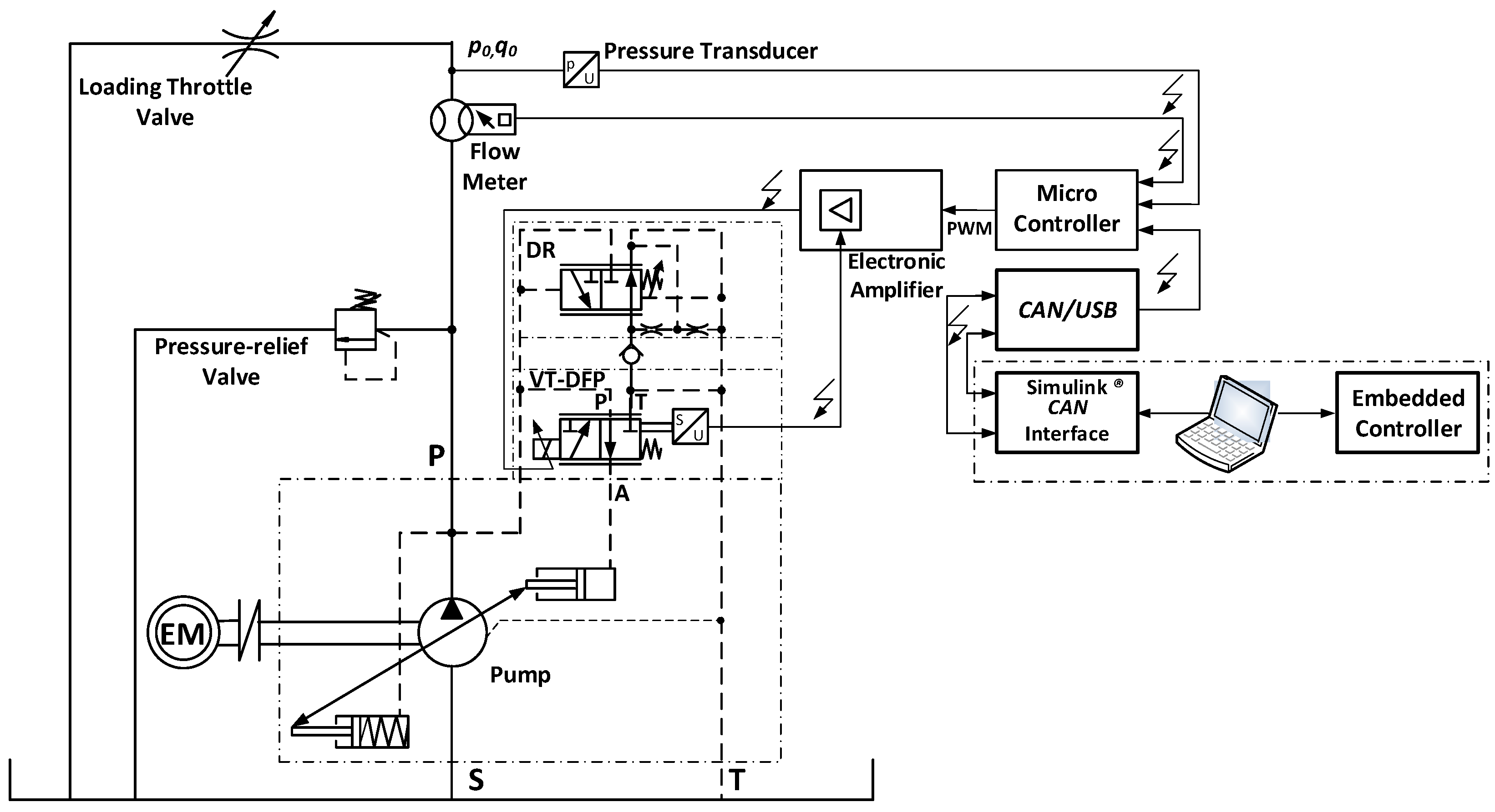
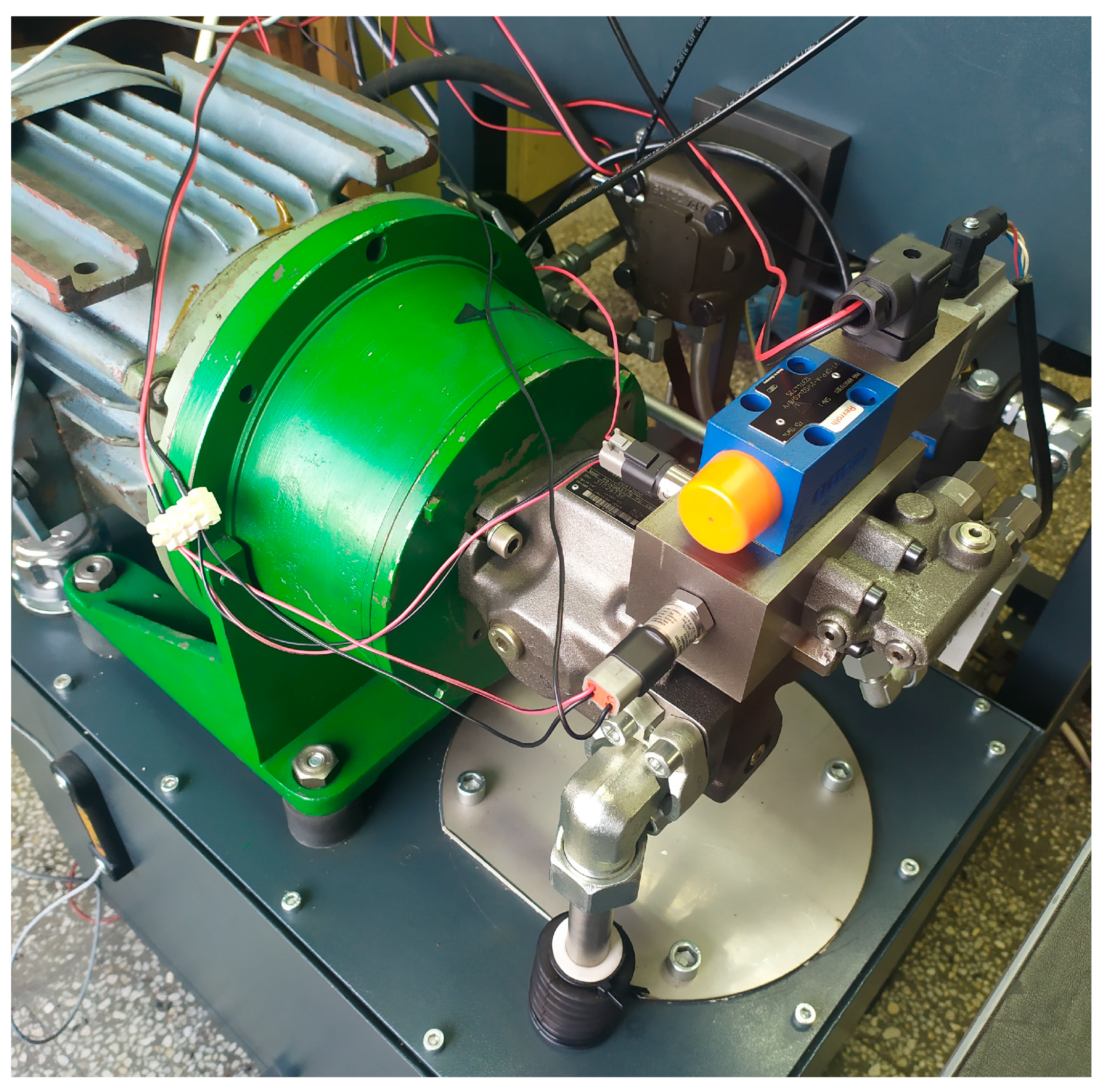
The article is organized as follows: Section 2 presents the design features of the plant and a rapid prototyping system for the implementation of various types of controllers. In Section 3, the plant model and adaptive controller design are shown; Section 4 presents the stability analysis of the designed adaptive controller; Section 5 presents the experimental study of the designed controller, and Section 6 contains short conclusions.

2. Plant Description

2.1. Variable Displacement Axial-Piston Pump

The plant of this study is a variable displacement axial-piston pump A10VSO (Bosch Rexroth AG, Lohr am Main, Germany). The pump is a swash plate type, and it is designed for hydraulic drive systems with open circulation. The longitudinal section views of the pump are depicted in Figure 1. This figure is a modified version of an existing image of this type of pump [52]. The flow rate of the pump is proportional to the rotation frequency and displacement volume. This allows a stepless regulation of the flow rate at a constant rotation frequency by changing the swash plate swivel angle. For this type of regulation between the pump and hydraulic cylinder or motor, a directional control valve is connected.

The classical hydro-mechanical pressure controller (type DR) is replaced with an electronically controlled 3/2 proportional valve 1 type VT-DFP [53]. The proportional valve (1) has an integrated inductive sensor (2). The sensor (2) is used for spool position feedback. The valve is intended only for that type of pump, and it is mounted on the hydro-mechanical controller plate. It operates as an electrohydraulic actuator for changing the swash plate’s (3) swivel angles. The swash plate swivel angle determines the pump displacement volume and the flow rate to the hydraulic system. The proportional valve (1) supplied the actuating piston (4), which is used to change the swash plate swivel angle.

When the swivel angle increases in the range of 0 to γ_max, the displacement volume also increases, and, hence, the pump flow rate. When the actuating piston (4) does not actuate the counter-piston (5), which has a spring (6), the swash plate (3) returns to the initial position corresponding to the maximal displacement volume. It is the same when the motor driving the pump is switched off. If the proportional solenoid (7) is not activated but the motor is switched on, then the pump is in the “zero stroke” mode (minimum displacement volume). This is a consequence of the fact that the proportional valve spool (8) is in a neutral position under the action of the force of the spring (9), and the discharge pressure of the pump acts on the actuating piston (4). The standby mode for this type of pump is achieved at 8–12 bar. At this value of pressure, there is an equilibrium between the force of the spring (6) acting on the counter-piston (5) and the forces of the actuating piston (4). This mode is typical for the switched-off electronic control of the proportional valve (1), in which the “zero stroke” is assumed. In most cases, the control device of the proportional valve (1) is an external electronic amplifier type VT-5041. The amplifier is implemented as a plug-in card in Euro-format. It is an analog-circuit-realized PID controller determining the parameters of the control signal to the valve solenoid (7) for the change in the swash plate swivel angle. The amplifier also processes the signals from the feedback on the position of the swash plate and the pressure in the pump discharge port. In contrast to the conventional system, in this study, the swash plate swivel angle sensor is replaced by a flow meter measuring the flow rate of the pump. The discharge pressure is measured by a pressure sensor connected to the pump output. The purpose is to provide feedback on the velocity and load by using a standard pump, which is not intended for secondary control [54]. In this case, the analog control function of the electronic amplifier is not used. It serves only as a power stage for driving the solenoid of the proportional valve.

2.2. Rapid Prototyping System for Real-Time Controllers

The experimental tests of the designed controller were carried out on an existing setup. This setup is part of the laboratory test rig. It allows a relatively easy and fast implementation of various real-time control algorithms [55]. A detailed description of the rapid prototyping system is presented in detail in a previous author’s article [56].

The hydraulic circuit diagram of the test system is depicted in Figure 2. The system has two main subsystems: hydraulic and control. The base of the hydraulic subsystem is a 130 L tank. The axial-piston pump A10VSO has a displacement volume of 18 cm³/rev. It is driven by a 7.5 kW electric motor with a 1500 min⁻¹ nominal rotation frequency. The pump displacement volume regulator is an electronically controlled proportional valve, type VT-DFP. In parallel to the regulator, a conventional hydro-mechanical pressure controller of type DR is connected. The DR regulator is connected by a custom-made hydraulic plate, and its intention is to protect the system from pressure overload. In the pump discharge pipeline, an additional direct-operated pressure-relief valve is connected. Moreover, a gear flow meter and a pressure transducer are connected in the pump discharge line. The measured flow rate (resp. velocity) and pressure (resp. load) act as feedback signals. The various load modes can be realized by a parallel-connected, precise hydraulic throttle check valve.

The key component of the control subsystem is a microcontroller type MC012-022 [57], which generates a control signal to the plug-in card amplifier type VT-5041, which controls a proportional valve VT-DFP solenoid [53]. The amplifier receives the feedback signal from a linear variable differential transducer (LVDT) integrated in the proportional valve. The USB/CAN interface type CG150 is used for the connection between the microcontroller and the portable workstation (PC). For code generation and the implementation of various control algorithms, the MATLAB/Simulink^® software product is used. The controller computes the control action value, which is applied to the plug-in amplifier. By the appropriately developed Simulink^® model, the control subsystem provides control in real time. The sample time is 0.01 s, which is sufficiently small to control the displacement volume of the pump. The realization of the laboratory experimental setup is depicted in Figure 3.

3. PI-Based Adaptive Actor–Critic Controller Design

The adaptive controller suggested in the article is from the class of so-called model-free controllers that do not require a plant model. Its parameters are tuned in real time on the basis of the initial conditions and measured data. The initial values of the controllers’ parameters must ensure the stability of the initial system. The structure of the developed closed-loop control system is presented in Figure 4.

It includes a plant to be controlled (axial-piston pump) and a PI-based adaptive actor–critic controller. The actor part of the controller ($K_a$) produces the control signal, which is the control action applied to the proportional valve solenoid, since the critic part of the controller ($K_c$) computes the system performance. The controller evaluates the flow tracking error as the difference between the desired pump flow rate and the measured pump flow rate. The tracking error and its integral are used as controller inputs. These two signals are utilized in the actor part to compute the proper control signal. The quality of the actor’s part is continuously computed by the controller’s critic part, which provides adaptive feedback for the real-time tuning of the controller parameters in order to improve the flow rate tracking performance and to optimize the adaptive controller.

3.1. Design of the Controller’s Actor Part $K_a$

The controller’s actor part is represented as an adaptive PI controller that evaluates the control signal $u$ from

$$u(k)=k_{p}e(k)+k_i{e}_{\mathrm{int}}(k),$$

(1)

where $e(k)$ is the tracking error and $e_{\mathrm{int}}(k)$ is the discrete-time integral of the tracking error. They are computed from

$$\begin{array}{l}e(k)=r_f(k)-y_f(k),\\ e_{\mathrm{int}}(k+1)=e_{\mathrm{int}}(k)+T_{0}e(k+1)-k_w\left(u(k)-u_{sat}(k)\right),e_{\mathrm{int},}(0)=0\end{array},$$

(2)

where $T_0=0.01 \mathrm{s}$ is the sample time and

$$u_{sat}(k)=\left\{\begin{array}{c}u(k),\hspace{1em}{u}_{\min }\le u(k)\le u_{\max }\\ u_{\max },\hspace{1em}u(k)>u_{\max }\\ u_{\min },\hspace{1em}u(k)<u_{\min }\end{array}\right..$$

(3)

The third term in the expression for the discrete-time integral of the error represents the anti-windup part of the adaptive PI controller that is realized as a condition of nonlinear feedback. The $u_{\max }=1000 \mathrm{mV}$ and $u_{\min }=0 \mathrm{mV}$ are the maximal and minimal admissible values of the control signal. The anti-windup coefficient is $k_w=0.1$. Its value is constant and is chosen experimentally in order to achieve a balance between the settling time and overshoot in the case of the saturation of the control signal. It should be noted that the achievement of saturation for $u(k)$ is an edge case and differs from normal operation. This is why, in the linear area of (3), the value of $u_{sat}$ is chosen to be equal to $u$. Introducing the anti-windup term in Equation (2) is needed to meet the requirements of industrial practice for the realization of the PID controller. The initial values of the PID controller parameters are chosen in a manner where the control signal does not achieve the maximum or minimum value. The values of the controller proportional gain $k_p$ and the controller integral gain $k_i$ are evaluated in real time in order to minimize the objective function $J(k)$ at each discrete $k{T}_0$ as

$$u^k=\arg \min J(u,k),$$

(4)

where $u^k$ is the control signal projection on the discrete time interval $(\begin{array}{cc}k{T}_0& \infty \end{array})$. The cost function is evaluated as

$$J(k)={\displaystyle \sum _{j=0}^{\infty }\frac{1}{2}}{\alpha }^j{e}^2(k+j),$$

(5)

where $\alpha \le 1$ is the discount factor. It can be seen from Expression (5) that the value of the cost function is unknown due to its dependence on future values of the flow rate error. Thus, the parametric approximation $\tilde{J}(k,p)$ of Function (5) can be used, where the tunable parameters are represented by vector $p\in R^2$, $p={\left[\begin{array}{cc}{k}_p& k_i\end{array}\right]}^T$. Approximation $\tilde{J}(k,p)$ depends implicitly on $p$ through control signal $u$. This approximation should fulfill the condition

$$\left|\tilde{J}(k,p)-J(k)\right|<\delta ,\hspace{0.33em}for\hspace{0.33em}k>k_0,\delta >0.$$

(6)

The PI controller can be regarded as a neural network with one linear layer and two weights $k_p$ and $k_i$. Then, the adaptive PI actor controller parameters can be tuned in real time by applying the backpropagation rule to the approximation $\tilde{J}(k,p)$ with respect to $k_p$ and the adaptive PI controller parameters are updated in real time according to

$$p(k)=\lambda p(k-1)+\Delta p(k),\hspace{1em}p(0)=p_0,\hspace{1em}\Delta p(k)=-l_p{\displaystyle \frac{\partial \tilde{J}(k,p)}{\partial p}},$$

(7)

where $\lambda$ is the forgetting factor and $l_p$ is the constant learning rate.

It should be noted that the adaptation of the parameters in (7) is stopped if the control signal achieves its maximal or minimal admissible value and adaptation starts again after the recovering of the control signal in the linear zone according to (3). This recovery appears with the help of the anti-windup term.

3.2. Design of the Controller’s Critic Part $K_c$

The approximated value $\tilde{J}(k,p)$ of the unknown cost function $J(k)$ is computed by the critic part of the controller. It is represented by an artificial neural network, which has one linear output layer and one hidden layer with a tangent hyperbolic activation function. The value of $\tilde{J}(k,p)$ is formed according to

$$\tilde{J}(k,p)=w_c{F}_{\sigma }(V_c,x),$$

(8)

where

$$x={\left[\begin{array}{ccc}e& e_{\mathrm{int}}& u\end{array}\right]}^T$$

(9)

is the input vector of the critic neural network. $V_c$ is the weight matrix of the hidden layer, with dimensions $2\times 3$. The activation function $F_{\sigma }$ is taken as the hyperbolic tangent function

$$F_{\sigma }(b)=\tanh 0.5b={\displaystyle \frac{1-e^{-b}}{1+e^b}}.$$

(10)

Function (10) is applied to two components of vector $b=V_{c}x$. The weights of the output layer form a row vector $w_c$ with dimensions $1\times 2$. In order to obtain a recursive form for the cost Function (5), the Bellman equation is represented in recursive form as

$$J(k)={\displaystyle \frac{1}{2}}{e}^2(k)+\alpha J(k+1).$$

(11)

For the approximation of $J(k)$ with $\tilde{J}(k,p)$ according to Equation (6), it is necessary for index $\tilde{J}(k,p)$ to minimize the Bellman error

$$\epsilon (k)=\left({\displaystyle \frac{1}{2}}{e}^2(k)+\alpha \tilde{J}(k+1,p)\right)-\tilde{J}(k,p).$$

(12)

As can be seen, the Bellman error represents the difference between $J(k)$ and $\tilde{J}(k,p)$ if the approximation $\tilde{J}(k+1,p)$ is “ideal” ($\tilde{J}(k+1,p)=J(k+1)$). Thus, the quadratic criterion is formed as follows:

$$J_c={\displaystyle \frac{1}{2}}{\epsilon }^2(k).$$

(13)

The minimization of Criterion (13) is a necessary condition to hold Expression (6) and it is used to tune the weights of the critic neural network in Equation (8). The parameters of the critic neural network $p_c$ are updated in real time by the following step:

$$p_c(k)={\lambda }_c{p}_c(k-1)+\Delta p_c,\hspace{0.17em}{p}_c(0)=p_{c0},\hspace{0.33em}\Delta p_c=-l_{p_c}{\displaystyle \frac{\partial J_c(k,p)}{\partial p_c}},$$

(14)

where ${\lambda }_c$ is a forgetting factor and $l_{p_c}$ is a constant learning rate.

3.3. PI-Based Actor Parameter Gradient Evaluation

It can be seen from Equation (7) that, for the adaptive PI controller parameter evaluation, the gradient of index $\tilde{J}(k,p)$ with respect to the general parameter $p$ is needed:

$${\displaystyle \frac{\partial \tilde{J}(k,p)}{\partial p}}={\displaystyle \frac{\partial \tilde{J}(k,p)}{\partial u}}{\displaystyle \frac{\partial u}{\partial p}},$$

(15)

where

$${\displaystyle \frac{\partial \tilde{J}(k,p)}{\partial u}}=w{G}_{\sigma }(V_c,x)V{\displaystyle \frac{\partial x}{\partial u}}.$$

(16)

The gradient $G_{\sigma }$ of Function (10) with respect to the vector $V_{c}x$ is evaluated by

$$G_{\sigma }(V_{c}x)={\displaystyle \frac{\partial F_{\sigma }(V_{c}x)}{\partial (V_{c}x)}}=0.5\left(1-F_{\sigma }^2(V_{c}x)\right)$$

(17)

and

$${\displaystyle \frac{\partial x}{\partial u}}={\left[\begin{array}{ccc}0& 0& 1\end{array}\right]}^T.$$

(18)

The derivatives of the control signal with respect to the PI controller parameters are

$${\displaystyle \frac{\partial u}{\partial p}}={\left[\begin{array}{cc}e& e_{\mathrm{int}}\end{array}\right]}^T.$$

(19)

3.4. Critic Network Parameter Gradient Evaluation

Expression (14) shows that, for the updating of the critic network weights, it is necessary to take the derivative of $J_c(k,p)$ with respect to the general parameter $p_c$,

$${\displaystyle \frac{\partial {\tilde{J}}_c(k,p)}{\partial p_c}}=\epsilon {\displaystyle \frac{\partial \epsilon }{\partial p_c}}=-\epsilon {\displaystyle \frac{\partial \tilde{J}(k,p)}{\partial p_c}}.$$

(20)

for $p_c=w_c$

$${\displaystyle \frac{\partial \tilde{J}(k,p)}{\partial w}}=F_{\sigma }(V_{c}x)$$

(21)

and for the $p_c=V_c$

$${\displaystyle \frac{\partial \tilde{J}(k,p)}{\partial V}}=w{G}_{\sigma }(Vx)x.$$

(22)

3.5. Initial Conditions

The initial conditions in this paper should be understood as the starting values of the adaptive controller’s parameters, especially the PI parameters

$$p\left(0\right)={\left[k_p\left(0\right),k_i\left(0\right)\right]}^T,$$

(23)

and critic network weights

$$p_c\left(0\right)={\left[V_c\left(0\right),w_c\left(0\right)\right]}^T,$$

(24)

and, together with the corresponding initial control law, they generate

$$u_0\left(k\right)=k_p\left(0\right)e\left(k\right)+k_i\left(0\right)e_{int}\left(k\right).$$

(25)

As stated, these values must be chosen so that the initial closed-loop system is stable before learning starts, in the sense of the bounded tracking error and control signal

$$\left|\left|e_0\right|\right|<B_e \mathrm{and} \left|\left|u_0\right|\right|<B_u<u_{sat},$$

(26)

because the subsequent adaptation is only guaranteed to preserve stability if it begins from a feasible stable policy. The theoretical reason for this requirement is that the controller is trained online by gradient descent and Bellman-error minimization, so the learning dynamics are local rather than global. Given that the adaptation process is asymptotically stable, which will be analyzed below in Theorem 1, we have the following:

$$\left|\left|p\left(k\right)-p\left(0\right)\right|\right|<{\delta }_{PI},$$

(27)

$$\left|\left|p_c\left(k\right)-p_c\left(0\right)\right|\right|<{\delta }_{cr}.$$

(28)

In other words, the algorithm does not promise that it can recover from arbitrarily bad initial parameters; instead, it assumes the initial condition lies inside a region where the closed-loop dynamics already behave acceptably, and the adaptation can refine the performance without destabilizing the plant. That is why the paper motivates the PI-actor simplification as a way to make good initialization easier.

A good rule is to initialize the actor with conservative PI gains that give slow but stable tracking, then initialize the critic so its value estimate is consistent with that baseline control policy. This reduces the mismatch between the current policy and the critic’s approximation, which helps avoid large Bellman errors at startup and prevents aggressive transient updates in the parameter space.

There is also a tradeoff between exploration and correction. If the initial controller is too conservative, then the system stays stable, but the signal variation may be small, which can slow parameter learning because the regressor excitation is weak. If the initial controller is too aggressive, then the adaptation spends its effort recovering from large transients instead of improving performance. Therefore, the best initial condition is usually one that is close enough to the desired operating regime to generate informative data, while still keeping the closed loop well-behaved. The values for the learning rates and initial parameters of the PI-based actor–critic system used in the experiment are presented in

Table 1. PIAC system parameters.

Parameter	Value
${\left[\begin{array}{cc}{k}_p(0)& k_i(0)\end{array}\right]}^T$	${\left[\begin{array}{cc}20& 500\end{array}\right]}^T$
Learning rate of the actor $l_p$	1
Forgetting factor of the actor $\lambda$	0.999
$V_c(0)$	$\left|\begin{array}{cc}0.001& 0.002\\ 0.002& 0.003\\ 0.001& 0.002\\ 0.001& 0.002\end{array}\right|$
Learning rate of the critic’s hidden layer	${10}^{-7}$
$w_c(0)$	${\left|\begin{array}{cc}1& 1\end{array}\right|}^T$
Learning rate of the critic output layer	${10}^{-2}$
Forgetting factor of the critic hidden layer	0.993
Forgetting factor of the critic output layer	0.999

.

The initial values for the PI controller parameters are chosen on the basis of a previously developed classical PI controller in order to ensure a stable transient response for the maximal load. The learning rates, forgetting factors, and initial weights of the critic neural network are chosen experimentally. Many experiments are performed, and the selected values of the learning rates and forgetting factors provide a compromise between the adaptation rate and stability. As can be seen in the next section, there is an upper bound for the learning rate. Exceeding this bound causes the instability of the closed-loop system.

4. Stability Analysis

The existing literature results for the stability analysis of control systems based on deep network dynamical programming generally use the Lyapunov criteria. However, the determination of the Lyapunov function is case-specific. Here, a brief analysis of the PIAC control system stability is presented.

Theorem 1. 

Let a continuous nonlinear system be given as

$$\dot{x}=f(x,u)$$

(29)

with  $f$  continuous on both $x$ and $u$, and control signal

$$u=g(x,p)$$

(30)

with $g$ continuous on both $x$ and $p$. Let the controller’s parameters $p$ be tuned by

$$\dot{p}=-l_p{\displaystyle \frac{\partial J}{\partial p}},l_p>0$$

(31)

where $J(t,p)$ is a smooth function on parameters for every $t$. Given that $x=0$ is an asymptotically stable stationary point of the closed-loop system for the initial values of parameters $p=p_0$, there exists an upper bound of learning rate $0<l_p<{\overline{l}}_p$ such that $x=0$ will remain an asymptotically stable stationary point for every $p(t),t>0$.

Proof. 

The possible candidate for the Lyapunov function of the closed-loop system is

$$V(x,p)=V_x(x)+{\displaystyle \frac{1}{2}}{p}^{T}p,$$

(32)

where $V_x(x)$ is positive definite. The time derivative of Equation (32) is

$$\dot{V}(x,p)={\displaystyle \frac{\partial V_x}{\partial x}}\dot{x}+p^T\dot{p}.$$

(33)

For $p=p_0=const$ , the system is asymptotically stable at $x=0$; therefore, the time derivative is

$$\dot{V}(x,p_0)={\displaystyle \frac{\partial V_x}{\partial x}}\dot{x}\le -\gamma {‖x‖}^2$$

(34)

for some $\gamma >0$ and $‖x‖<\delta$ . Taking into account Equations (31) and (34) and due to the continuity of Equation (33), we have the following for $p(t)$ , where $‖p(t)-p_0‖<{\delta }_p$ ,

$$\dot{V}(x,p)=-\gamma {‖x‖}^2-l_p{p}^T{\displaystyle \frac{\partial J}{\partial p}}.$$

(35)

Let $\alpha ={\max }_{p,t}‖{\displaystyle \frac{\partial J}{\partial p}}‖>0$ . Then, it follows that

$$\begin{array}{l}\dot{V}(x,p)\le -\gamma {‖x‖}^2-l_p{p}^T\alpha \Rightarrow \\ \dot{V}(x,p)\le -\gamma {‖x‖}^2+l_p\alpha ‖p‖\end{array}.$$

(36)

To provide $\dot{V}(x,p)\le 0$ , it is sufficient that

$$l_p\alpha ‖p‖\le \gamma {‖x‖}^2.$$

(37)

Inequality (37) holds if

$$l_p<{\displaystyle \frac{\gamma {‖x‖}^2}{\alpha ‖p‖}}<{\overline{l}}_p,$$

(38)

where

$${\overline{l}}_p=\underset{x,p}{\min }{\displaystyle \frac{\gamma {‖x‖}^2}{\alpha ‖p‖}}.$$

(39)

Therefore, for $l_p<{\overline{l}}_p$ , $\dot{V}(x,p)<0$ , which provides the stability of the closed-loop system. □

Equation (38) represents a compromise between the speed of adaptation, which depends on the learning rate, and the closed-loop system stability. A larger learning rate leads to fast adaptation but can cause the instability of the control system, since a slow learning rate will ensure stability at the expense of slow adaptation and control performance. Expression (39) ensures a learning rate upper bound that provides stability during adaptation.

The above theorem provides only a local stability analysis, and it holds if the adaptation starts from the initial parameters, providing an asymptotically stable initial system. Moreover, the theorem not only guarantees asymptotic stability for the system state $x$ but also guarantees the asymptotic stability of parameters $p$. Since the controller parameters and system states are interdependent, the Lyapunov function (32) is representative of the autonomous closed-loop adaptive system.

Corollary 1. 

The parameters’ vector $p(t)$in Theorem 1 remains bounded and asymptotically stable for $p=0$.

Proof. 

It follows from the negative definiteness of the derivative of $V(x,p)$  with respect to t for a bounded learning rate. □

Although, from a practical point of view, the experimental implementation uses a fixed-step discrete-time realization for the integral action and parameter updates, the underlying plant dynamics remain in continuous time. Therefore, the theorem is stated in continuous time to analyze the ideal closed-loop adaptive dynamics, while the discrete-time implementation is understood as a sampled-data approximation of that design. Therefore, under a sufficiently small sampling time, the discrete-time controller approximates the continuous-time law and preserves the intended stability properties.

5. Experimental Study

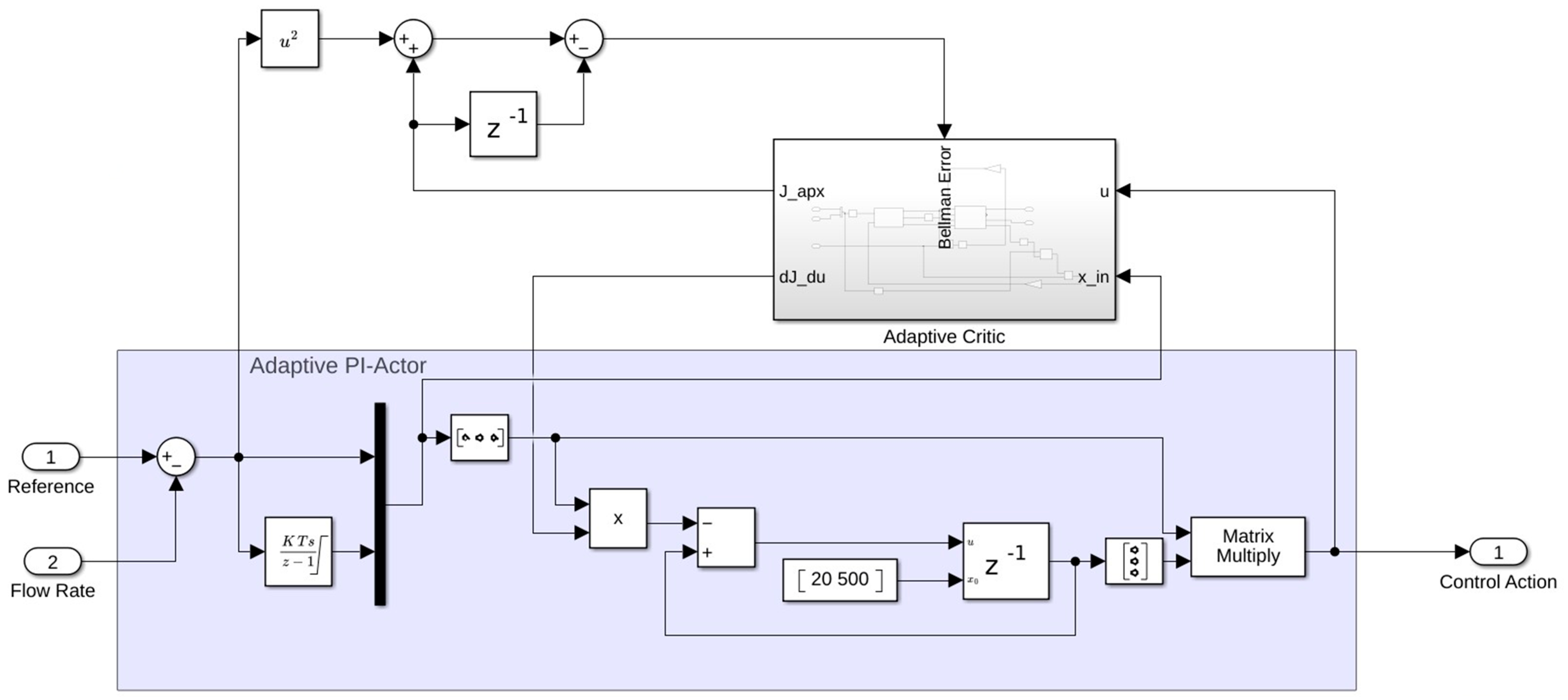
The proposed PI-actor–critic controller is realized as a fixed-step, discrete-time Simulink model that includes separate actor and critic subsystems, along with the routines for gradient evaluation and parameter updating (Figure 5). The tunable weights are implemented through an integer delay element combined with a summing block in the feedback loop, which enables the weights to be refreshed at every simulation step. Network activation is computed by multiplying the input vector by the weight matrix, followed by the element-wise application of the tanh function in the hidden layer. The precomputed gradient formulae are then implemented using standard mathematical blocks to generate corrective feedback signals for updating the weights.

This AC controller model is suitable for both the offline numerical simulation and automatic generation of C or ST code from Simulink^®, which can then be deployed on a microcontroller or PLC. For rapid prototyping, it can also run in real time, with CAN communication established between the host PC and the industrial MC012-022 microcontroller, which acts as a bridge for the measured pressure, flow rate, and LVDT signals while also issuing the PWM command to the pump actuator. The proposed PIAC controller is represented by a 13-state nonlinear model, which is of a relatively modest order. By comparison, previously designed H∞ and μ-controllers had 11 and 21 states, respectively, and required suitable nominal and uncertainty models to ensure closed-loop robustness. Implementing controllers of this complexity in industrial PLCs or embedded microcontrollers is generally feasible at sample rates above 1 ms. Computational latency is managed by the PLC real-time operating system (RTOS) to guarantee the fulfillment of the sample time constraints. In the case of PIAC, the computation is bound to a fixed number of basic floating-point arithmetic operations dependent on the number of neurons in the critic network.

The flow rate in the system is measured by a gear flow meter QG100 with an operating range up to 70 L/min and working pressure up to 42 MPa. The gear’s rotation is detected by a magnetic Hall encoder generating one pulse per tooth. The encoder signal is processed by the microcontroller to convert the number of pulses per second to liters per minute, taking into account the number of teeth of the gear flow meter. The PWM signal used to drive the pump actuator is operating at a 1 kHz carrier frequency. Additional details on the technical specifications of the sensors and test bench setup can be found in [56].

To assess and compare the performance of the Adaptive PI-based actor–critic controller, we define a sum of square error (ISE) $err$ and sum of absolute error (IAE) $er{r}_u$ as

$$er{r}_{ise}={\displaystyle {\displaystyle \sum _{k=t_0}^{t_f}}e{(k)}^2},\hspace{0.17em}er{r}_{iae}={\displaystyle {\displaystyle \sum _{k=t_0}^{t_f}}\left|e(k)\right|}$$

(40)

Table 2. Performance index ISE of control systems with various controllers.

Controller	$\mathit{e}\mathit{r}{\mathit{r}}_{\mathit{i}\mathit{s}\mathit{e}}$
	Loading 2	Loading 3	Loading 4	Loading 5
LMRAC	1354.3	1442.3	1119.1	791.7
PI	1668.1	2620.3	2522.4	1397.8
PIAC	808.7	1230.2	762.1	578.0
AC	914.7	1229.7	831.7	605.3

reports a performance index ISE for four controllers across four loading conditions, so it summarizes the cumulative control quality rather than only the transient behavior. Since smaller values are better, the table directly supports a comparison of the regulation efficiency under different loads. For LMRAC, the performance is good and consistent, but not the best (between 791 to 1354 from loading 2 to 5), so it is clearly better than PI but worse than PIAC and AC. This suggests the Lyapunov-constrained adaptive law is robust, but is less aggressive in minimizing the quadratic cost than the critic-based methods (the critic-based controllers reduce the value of the ISE index by more than 30% for maximal loading 2 in comparison to the ISE index for LMRAC and more than 20% for minimal loading 5). For PI, the values are the largest in every case, between 1397 to 2620, which means the classical controller is the weakest performer under all loads, especially loading 3 and 4. That indicates the fixed-gain PI law cannot sufficiently compensate the pump’s nonlinear load dependence. For PIAC, the results are between 578–1230, so it gives the lowest cost across all loadings. AC is the second-best and very close to PIAC with 605–1229. Therefore, the adaptive-critic structure is still much better than LMRAC and PI. The PIAC improvement over AC shows that the PI-based actor improves the learning efficiency and reduces the cost compared with a generic actor–critic structure. The results for index IAE in

Table 3. Performance index IAE of control systems with various controllers.

Controller	$\mathit{e}\mathit{r}{\mathit{r}}_{\mathit{i}\mathit{a}\mathit{e}}$
	Loading 2	Loading 3	Loading 4	Loading 5
LMRAC	913.7	844.9	687.7	659.4
PI	1059.0	1271.1	1213.9	963.2
PIAC	685.3	805.1	554.6	584.8
AC	760.7	750.7	609.8	603.0

are almost the same. The difference between the values for various controllers is smaller than the ones for ISE, because the ISE penalties include more large errors than smaller errors.

Table 4. Settling time of control systems with various controllers.

Controller	${\mathit{t}}_{\mathit{s}\mathit{t}},\mathit{s}$ (Increasing Reference)				${\mathit{t}}_{\mathit{s}\mathit{t}},\mathit{s}$ (Decreasing Reference)
	Loading 2	Loading 3	Loading 4	Loading 5	Loading 2	Loading 3	Loading 4	Loading 5
LMRAC	0.9	0.4	0.3	0.4	0.9	0.5	0.4	0.4
PI	2.5	1.5	1.3	1.5	1.5	1.7	1.3	1.7
PIAC	0.5	0.4	0.3	0.4	0.45	0.3	0.3	0.4
AC	0.5	0.3	0.3	0.4	0.5	0.3	0.3	0.3

compares the transient performance across controllers and load cases, and the numbers clearly show how adaptation improves the speed of the response. The PIAC has the fastest transient response overall; mostly, the settling time is between 0.3 and 0.5 s, while PI is consistently the slowest, reaching a settling time of 1.3–2.5 s depending on loading and direction. For LMRAC, the settling times are good but not the best: 0.9, 0.4, 0.3, and 0.4 s for the increasing reference and 0.9, 0.5, 0.4, and 0.4 s for the decreasing reference. This means the Lyapunov-based adaptive law is stable and reasonably fast, but it does not provide the quickest transient recovery in comparison to the other adaptive methods. For PI, the response is the slowest in both directions, especially at loading 2, where it takes 2.5 s for the increasing reference and 1.5 s for the decreasing reference, and it remains above 1.3 s even in cases with smaller loads (loading 4 and loading 5). This suggests the fixed-gain PI controller is less able to handle the changing pump dynamics and load dependence. For PIAC and AC, the settling times for both directions are the shortest for all loadings, and the variations in the settling time for the smallest and largest loadings are small (the settling times for the increasing reference are 0.5, 0.4, 0.3, and 0.4 s and for the decreasing reference are 0.45, 0.3, 0.3, and 0.4 s). This indicates that the generic actor–critic is very responsive and the PI-based actor–critic keeps nearly the same speed with a simpler actor structure that is more appropriate for practical realization.

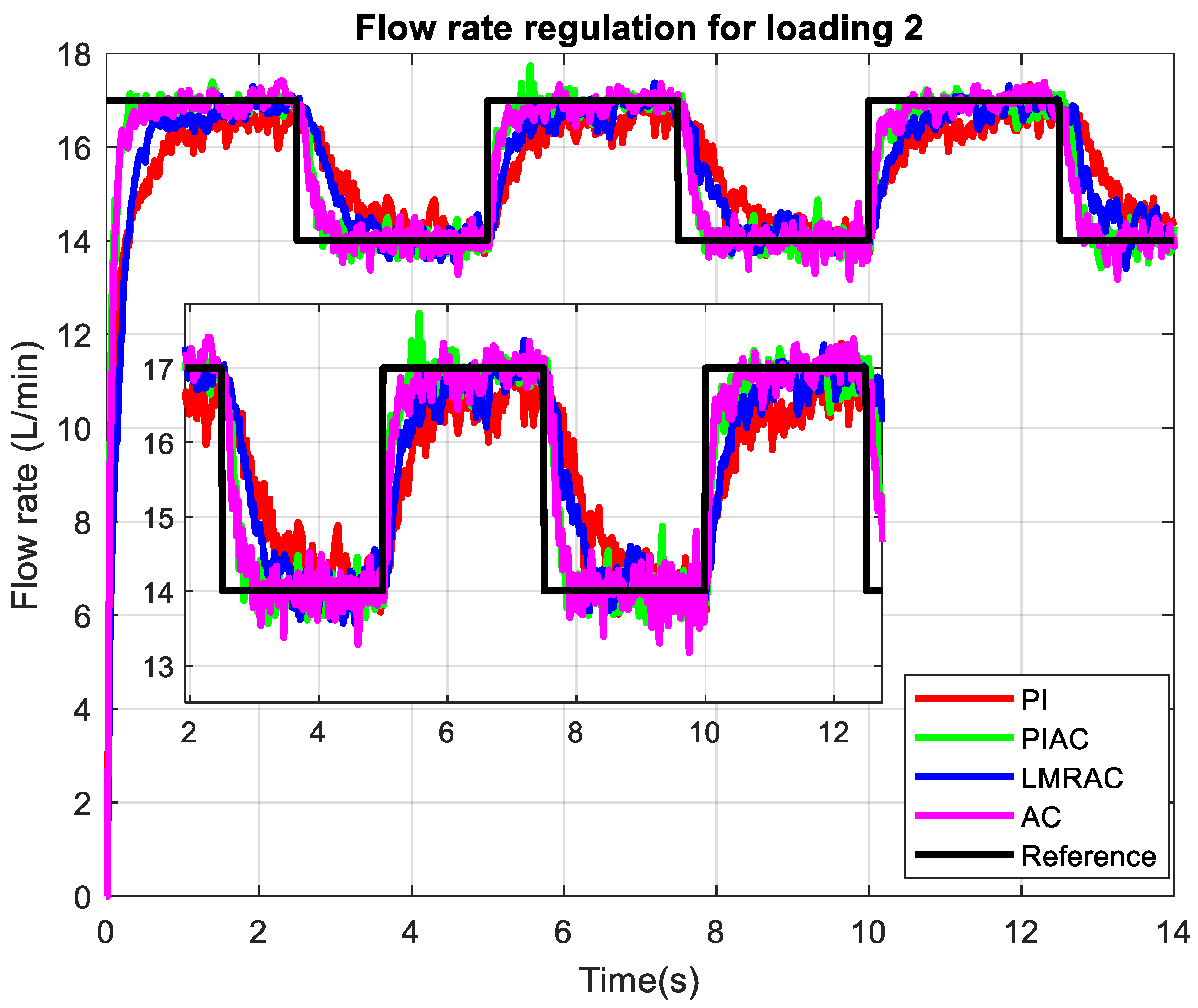
Figure 6 shows that the proposed controller can track the flow reference under the most demanding load. Loading 2 corresponds to the smallest throttle valve opening, effectively shunting the pump and creating loading pressure near the relief valve threshold of 100–120 bar. The hydraulic resistance is the highest, so the pump is working against the largest load disturbance. This is the case where the plant response is also the most challenging from a control theory point of view. The red PI curve has the largest deviation during the setpoint transitions, with a settling time of nearly 2.5 s (five times larger than the settling time for ACPI) and a pronounced steady-state error of 0.5 L/min in some of the steps, indicating that the calculated control effort is not enough. This steady-state error occurs because the time between switching the reference signal is larger than some of the settling times for the system with the PI controller. Certainly, the PI controller can be returned to behaving better for this loading, but this will lead to worse tuning over the whole loading range. A classical PI law has no mechanism to retune its gains online, so, under high load, it typically shows a slower settling time when the effective plant dynamics are changed.

In the highest loading regime, the PIAC and AC traces track the 14–17 L/min reference with a visibly smaller integral square error than PI and a roughly comparable or slightly better settling time than LMRAC. This suggests that the adaptive control laws are successfully reshaping the control gains online to compensate for the heavy-load nonlinearity, whereas the classical PI is more sensitive to the gain mismatch induced by the high load. The settling time for PIAC and AC is around 200 ms, while the LMRAC goes toward 300–400 ms. 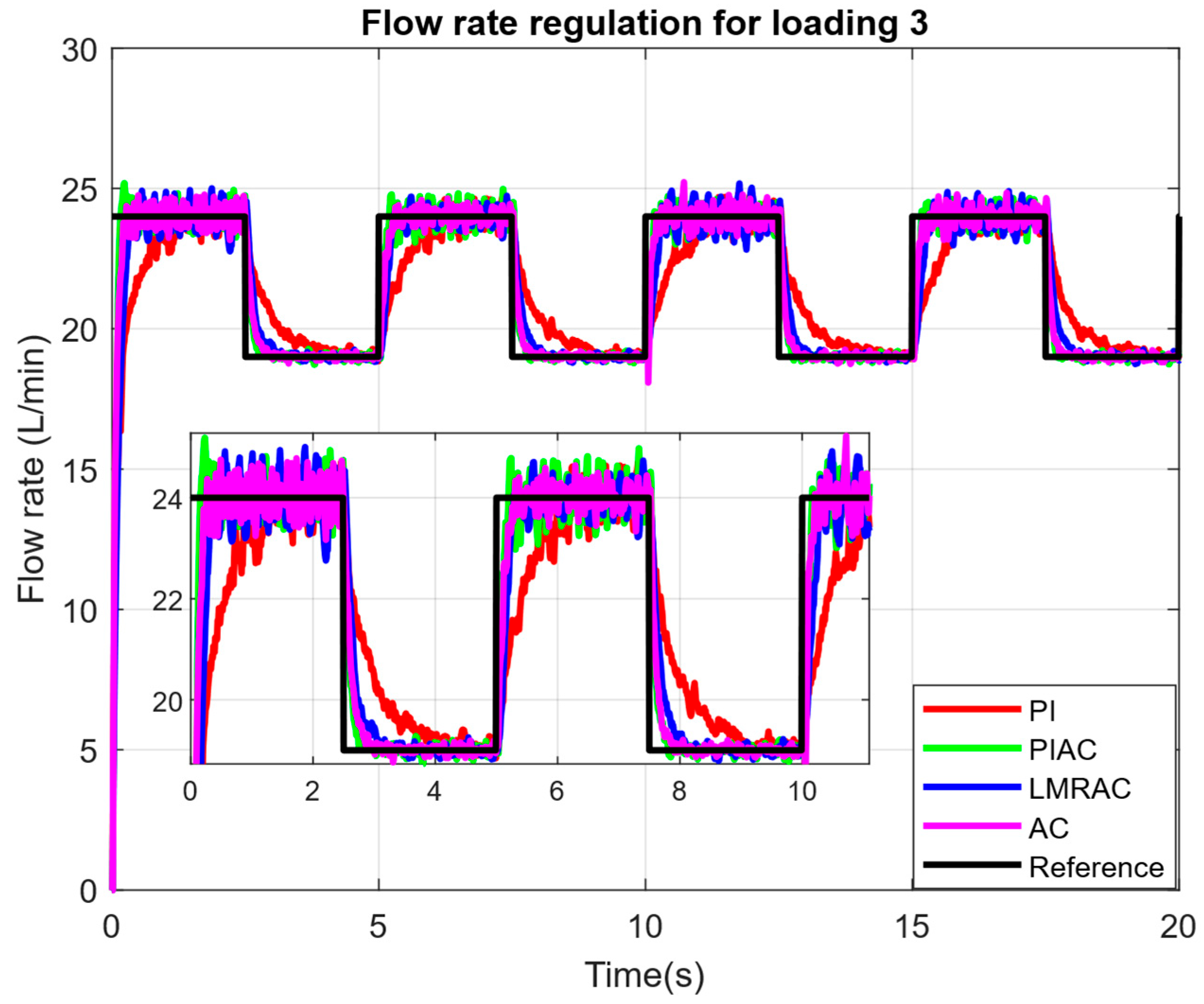At loading 3 (Figure 7), the reference levels are between 19 and 24 L/min, and all four controllers track them reasonably well, as expected because the load is lower than at loading 2. However, the PI curve shows the largest lag and undershoot, while PIAC, AC, and LMRAC stay much closer to the reference with only small integral square errors around the switching instants. This indicates that the adaptive-critic schemes still preserve an advantage in transient shaping. The PIAC and AC responses appear slightly tighter around the 24 L/min plateau and recover faster near the 19 L/min level, consistent with online parameter adjustment and value-based correction; LMRAC is also strong, suggesting its Lyapunov-constrained adaptation remains effective in this moderate-load regime. The settling time for the adaptive controller is even shorter than loading 2, going toward 300 ms in some of the steps. Moreover, we see a noticeable reduction in the steady-state oscillations for adaptive controllers as the experiment progresses.

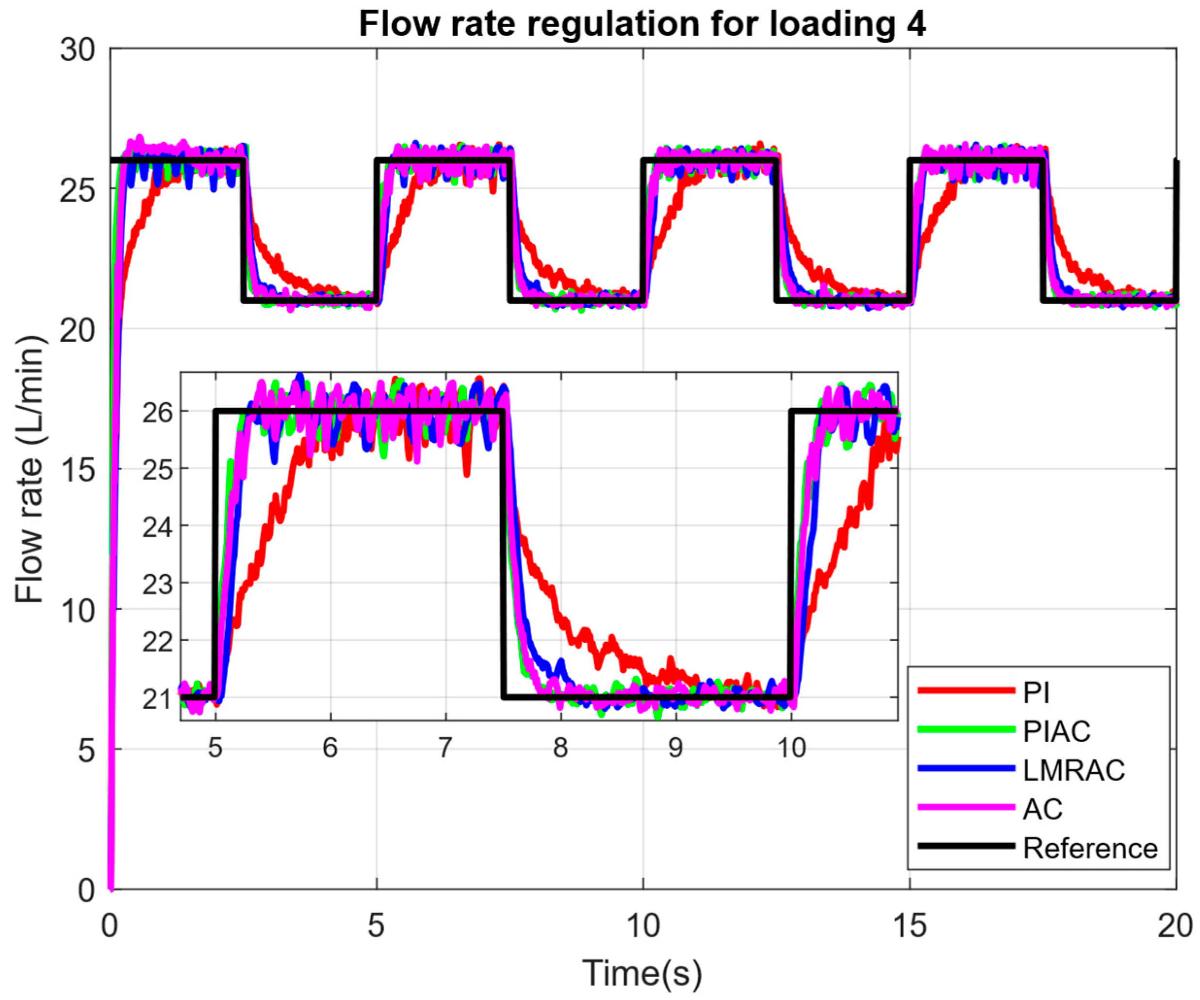
At loading 4 (Figure 8), the reference is around 26 L/min on the high level and 21 L/min on the low level, and all controllers track these steps fairly well, reflecting the easier dynamics under a lower load. The PI response is still the slowest (approximately 1.3 s), with a noticeable lag and undershoot after the drop toward 21 L/min, while PIAC, AC, and LMRAC stay much closer together and settle faster (for the three adaptive controllers, the settling time is 0.3 s). From a control-theory standpoint, this is what one would expect as the load decreases: the plant becomes less stressed, so tracking improves and the controller needs less corrective effort. The adaptive-critic methods still show their advantage in transient suppression, with PIAC and AC appearing slightly tighter around the step edges, while LMRAC remains competitive but not clearly better; this suggests the learned policy is handling the remaining nonlinearities effectively even though the baseline difficulty is reduced.

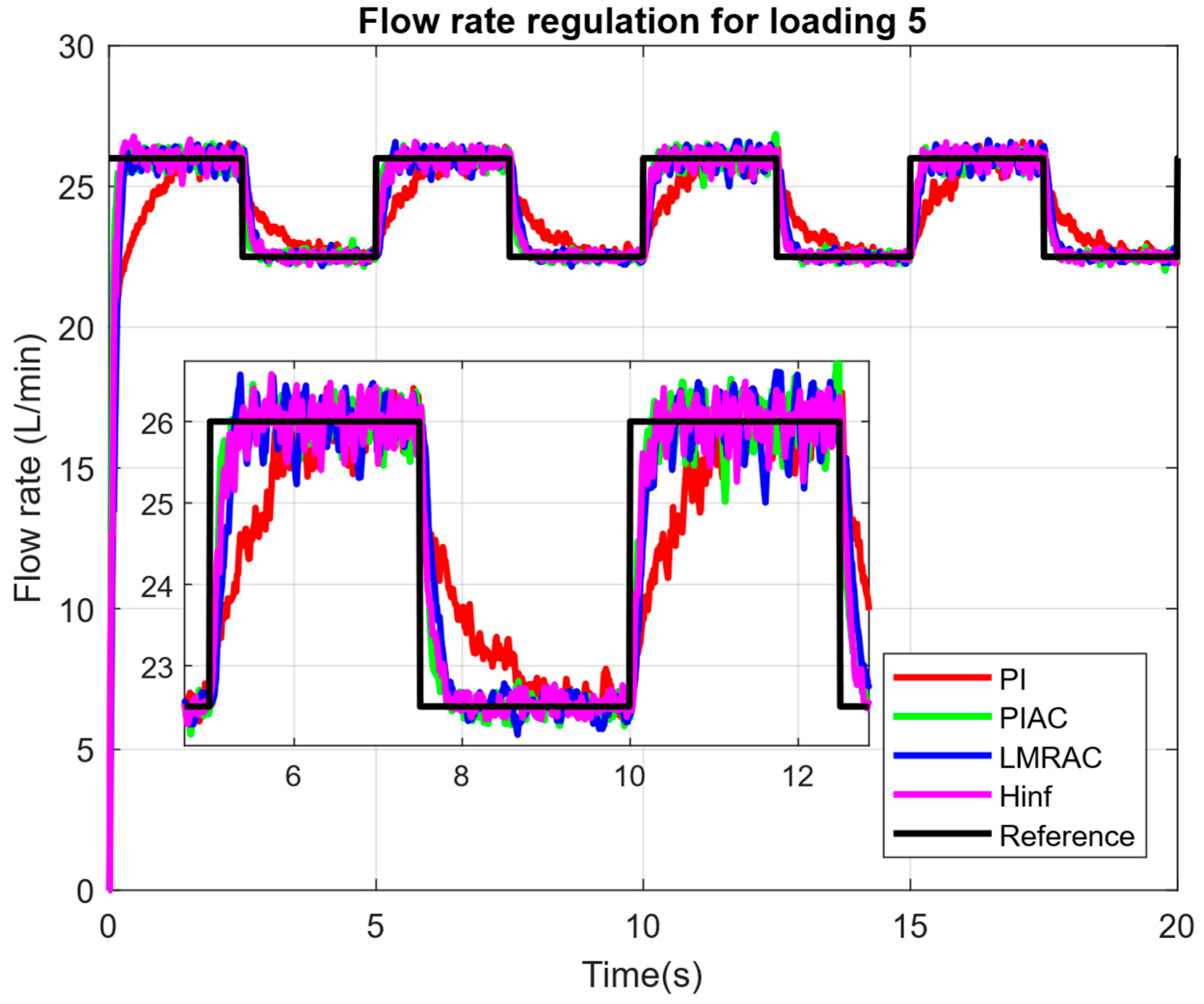
The least resistance at the pump is established with a throttle valve setting at 5 mm, corresponding to the results presented in Figure 9. At this setting, the pressure output is reduced to 20–30 bar, and the flow rate can reach as high as 26 L/min. As in previous cases, we see that PI tunings are most conservative with very long settling times above 1.5 s. The adaptive controllers are tightly stacked together with quick adaptation from the initial conditions. Most notably, we see that the change from AC to PIAC does not significantly change the performance of the closed-loop system. Moreover, it should be noted that all controllers provide flow rate transient responses without overshoot. The flow rate crosses the reference value due to the sensor noise.

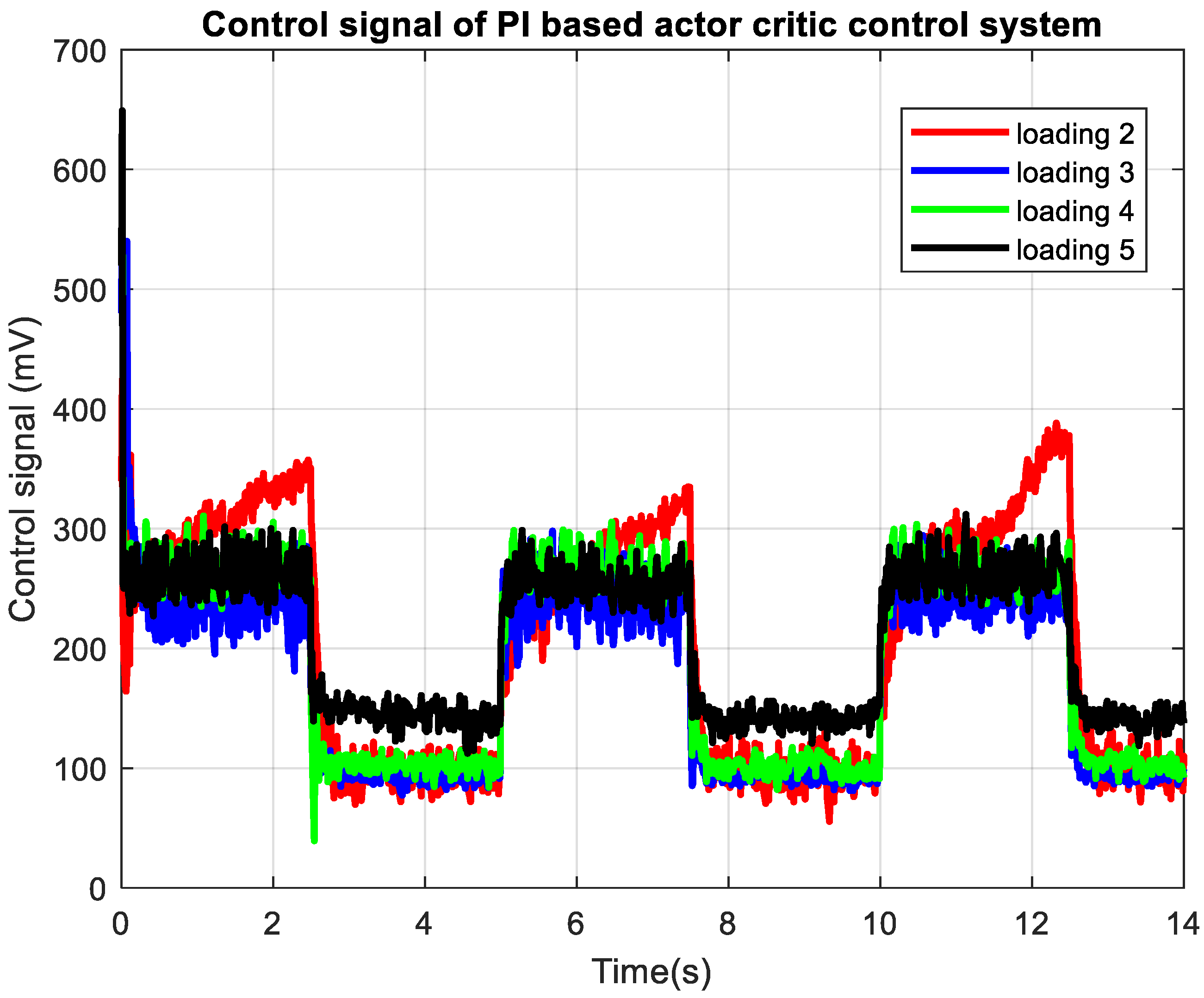
The control effort for the PIAC over changing loading conditions is compared in Figure 10. The meaning of the control signal is a PWM voltage waveform toward the amplifier stage of the solenoid-driving proportional valve, which indirectly drives, in turn, the pump swash plate swivel angle. All signals vary in similar ranges, and, as expected, oscillations in control signals are higher than in output signals. What is notable is the behavior at loading 2, where the PIAC is generating increasing control action near the steady state, reflecting the limiting behavior of the relief valve acting on this loading level between 100–120 bar, which is not present at lower loadings. Moreover, the lower level during loading 5 is higher than the control actions for other loading conditions, which indicates the nonlinear steady-state gain of the pump output in relation to the control valve action.

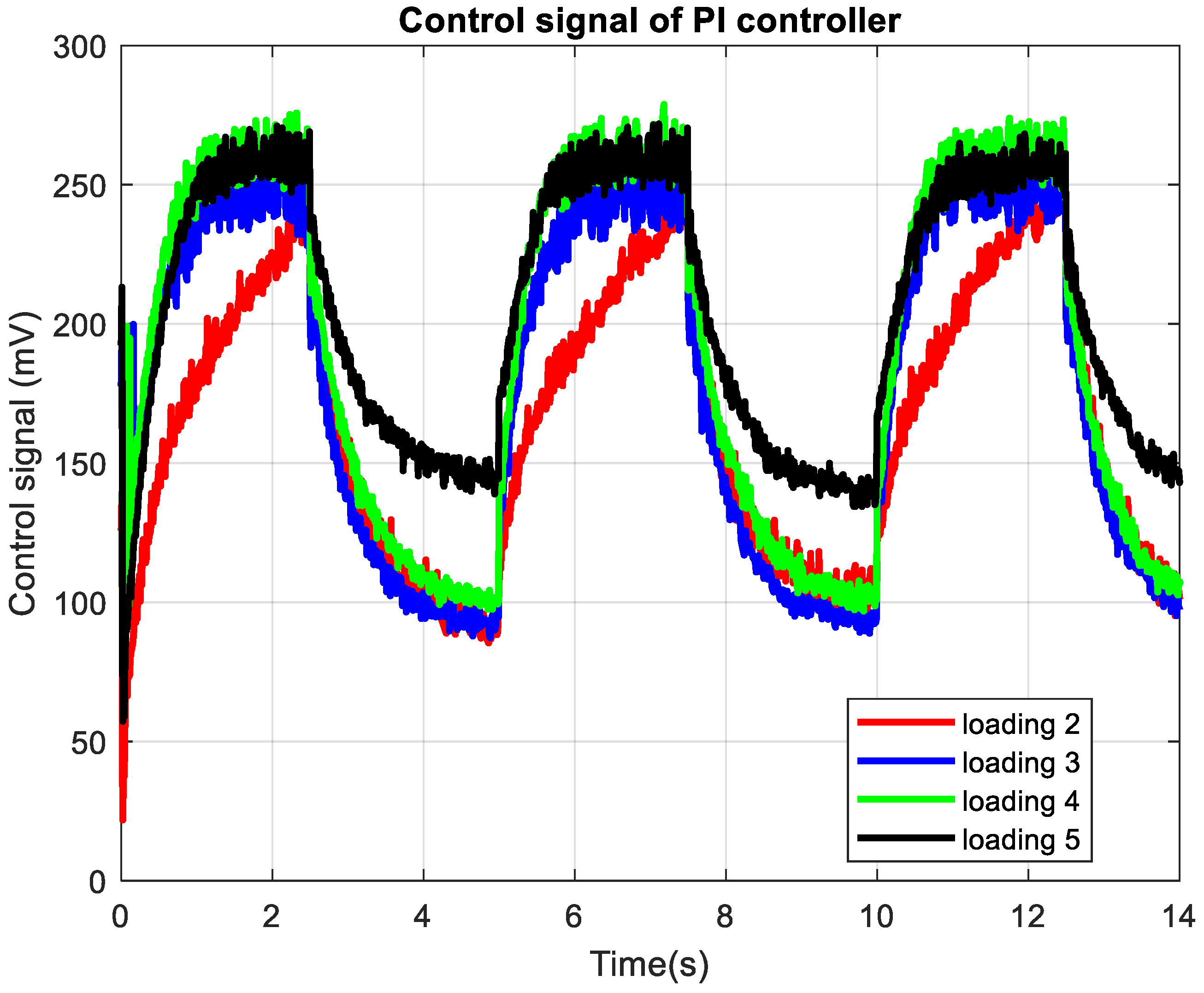
In Figure 11, we also analyze the control signals with the conventional PI controller. As mentioned, it works with fixed gains tuned conservatively to allow robust performance over the full range of loading. The most notable difference is that PIAC is able to reach higher control levels above 300 mV, with PI reaching no more than 270 mV, which proves the larger margin of control for PIAC. Contrary to PIAC behavior at the highest loading 2, the conventional PI uses the least control action with the most delayed waveform compared.

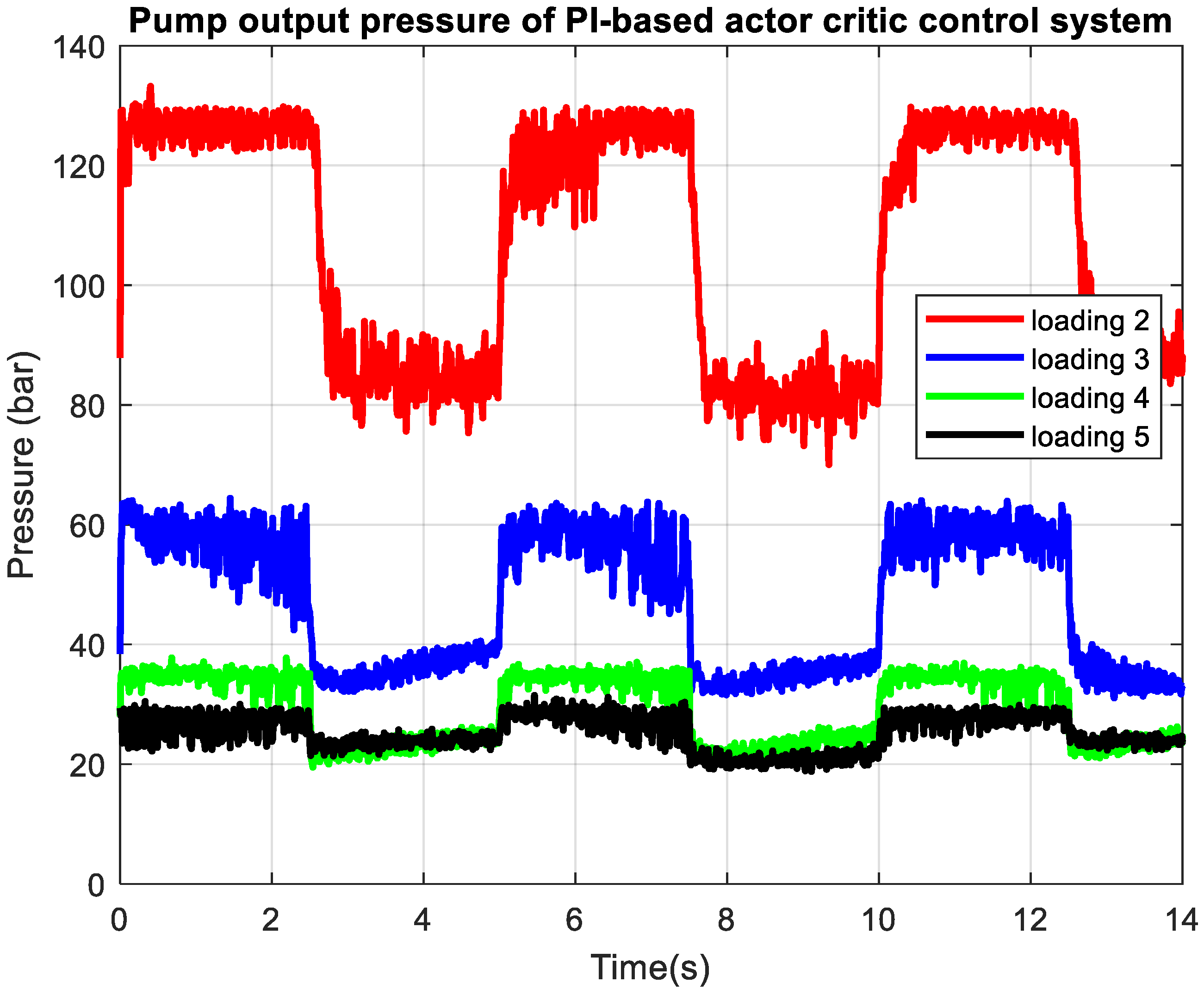
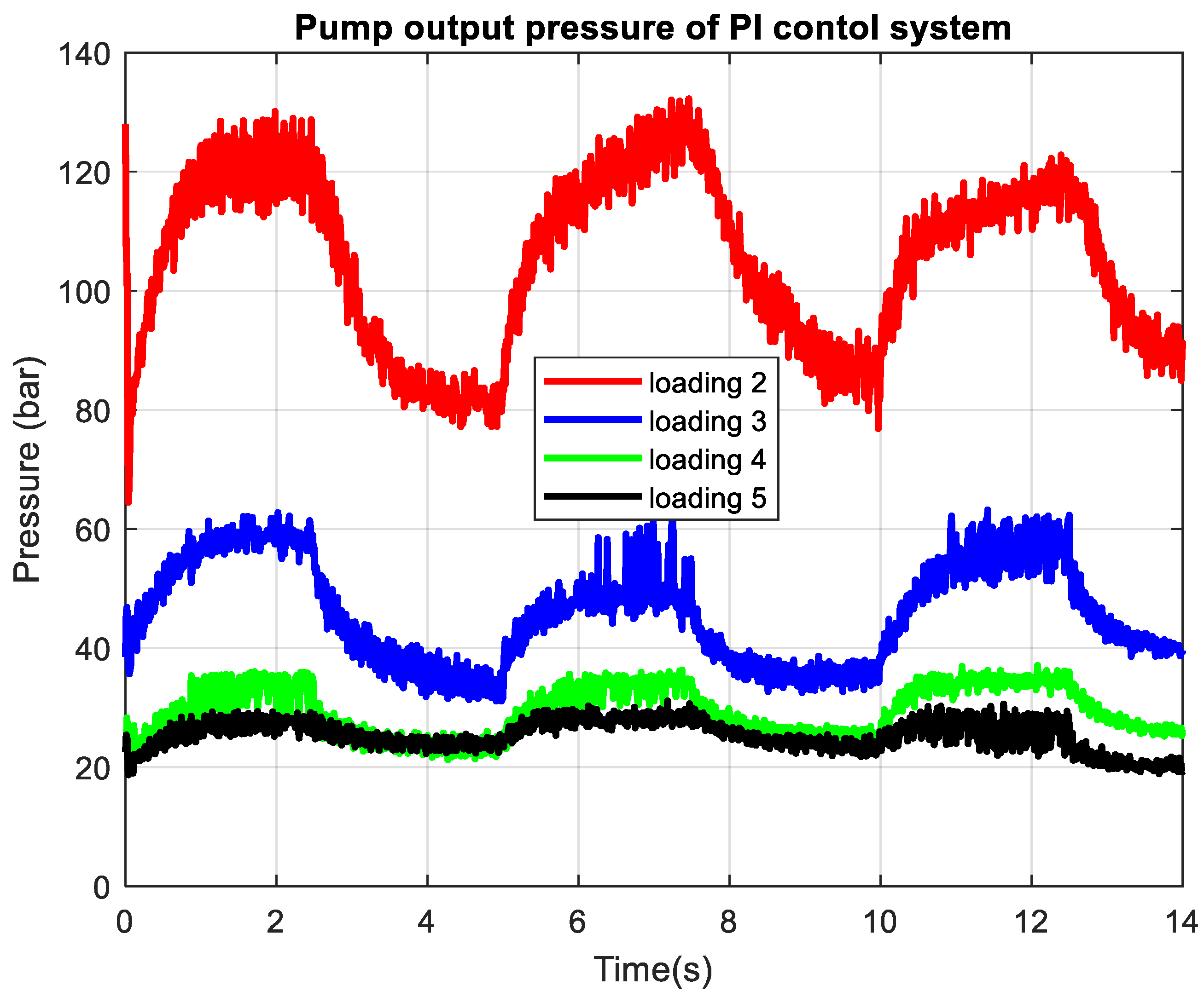
Then, in Figure 12, we examine the static pressure measured at the pump outlet, where we can track the resistance range created by the throttle valve. As noted, loading 2 is creating pressure in the range between 80 to 130 bar, loading 3 is giving between 35 to 60 bar, loading 4 is 20 to 35 bar, and loading 5 is mostly steady around 20 bar. It is evident that the proposed loading approach is able to explore the full working range of the axial-piston pump, and PIAC is able to perform consistently. In Figure 12, we see that steady-state oscillations of the pressure signal increase with the loading level, which is expected due to the increased energy dissipation at the higher power output, but we also see that the adaptive action of the controller can reduce the occurrence of oscillations with time, supposedly due to the presence of the pressure dimension in the critical domain.

For comparison, we show, in Figure 13, the behavior of the pressure signal for the system with a conventional PI controller, where, generally, the range of the pressure for the loading levels is preserved, but the waveform follows a different pattern determined by the corresponding flow rate and pressure/flow pump characteristics. Despite the conservative tunings of the PI, which do not aim to demonstrate exceptional tracking in the flow rate, the pressure oscillations are considerable compared to the PIAC, especially for loading 2 and 3.

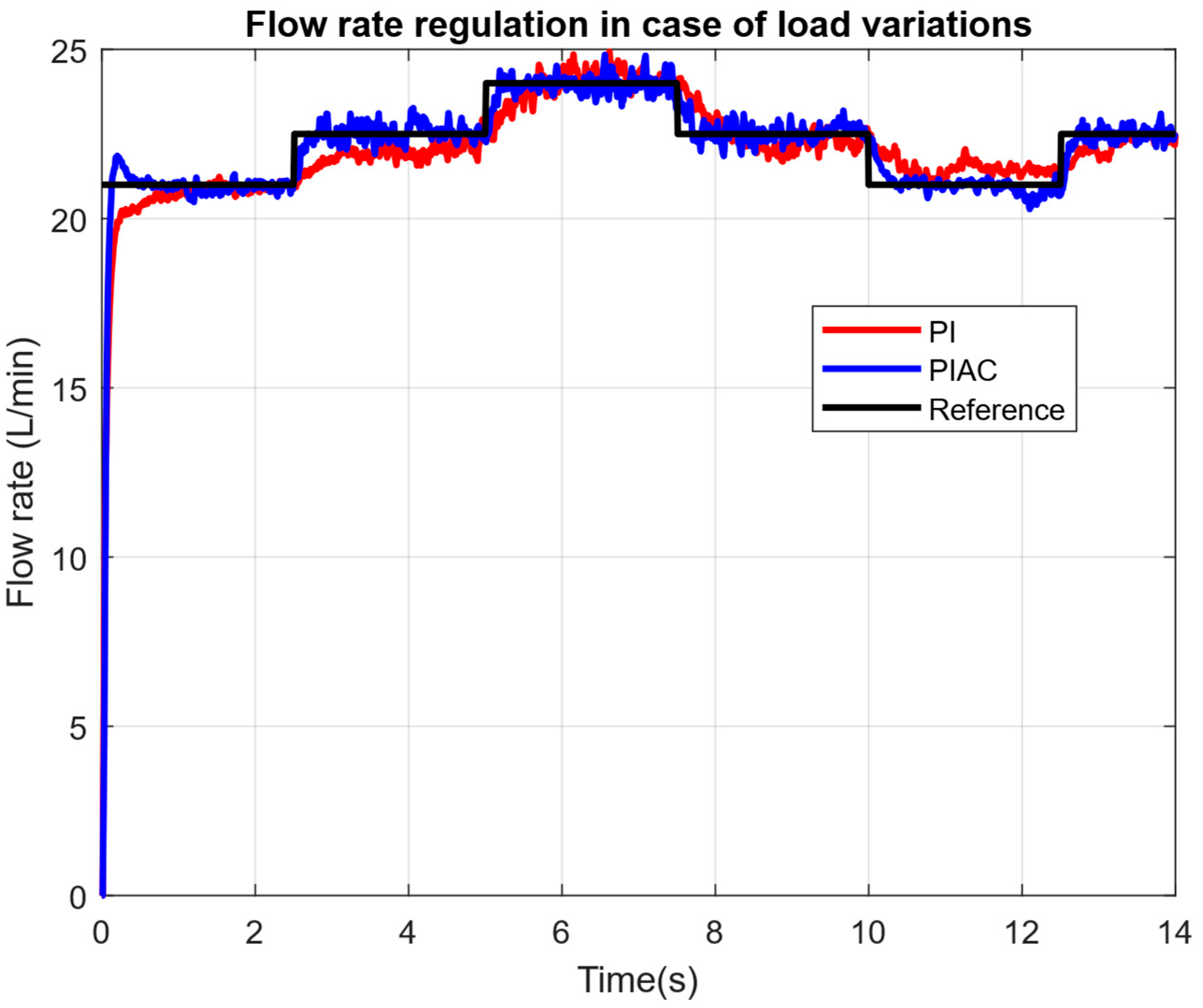
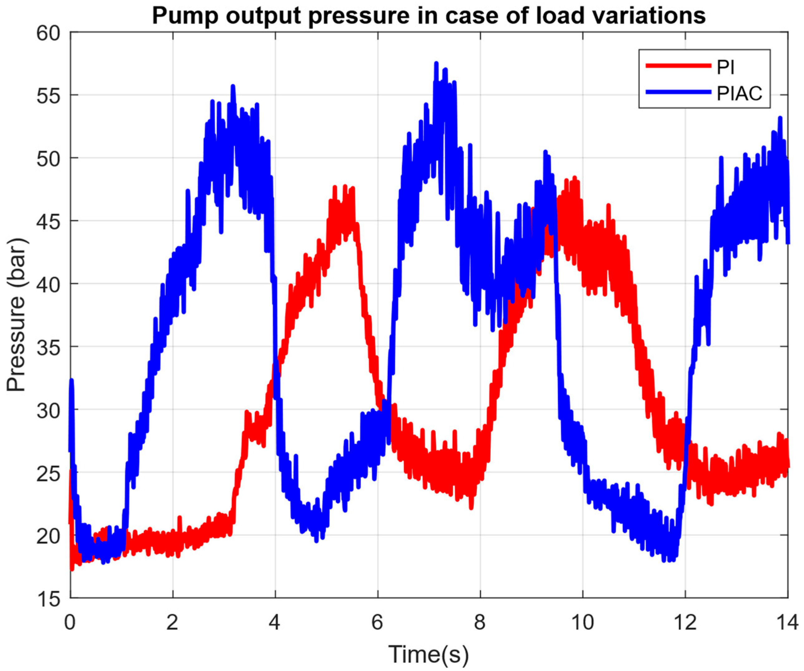
Additionally, we examine the behavior of the closed-loop system under dynamic load variations. In this experiment, we have a predefined reference signal with three levels of 21, 22, and 24 L/min (Figure 14), and, at the same time, we add random load variation by changing the throttle valve opening between 20 and 55 bar (Figure 15).

As evident in Figure 14, the PIAC controller is able to keep the system insensitive to dynamic load variations without evident deviations from the prescribed trajectory, except for the step transients and steady-state oscillations. 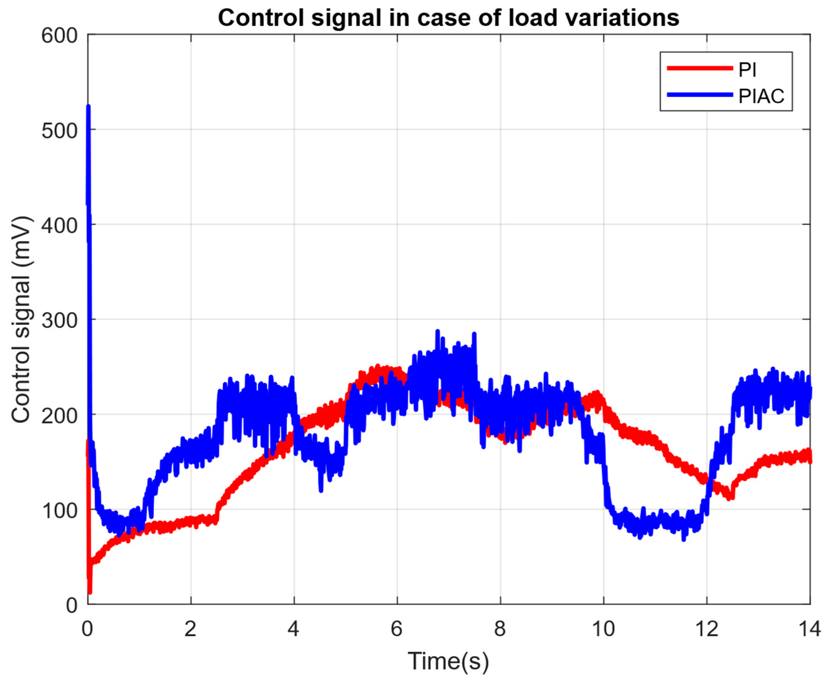However, in the case of the PI controller, we see a notable steady-state error between the 2nd and 5th second and between the 10th and 12th second, in relation to the loading changes in Figure 15. The control signals of both controllers in the dynamic loading experiment are compared in Figure 16, where we see that PIAC operates over a higher bandwidth with steeper slopes and steady-state reactivity in response to dynamic loading.

The results for the flow rate control from both experiments show that the transient responses for PIAC are without overshoot, and, in the case of different loading, the settling time is up to 0.5 s, while the settling time for the classical PI is up to 2.5 s. Moreover, it is seen that these results are obtained in the presence of significant measurement noise. Moreover, during the experiments, the temperature of the fluid is increased, which is a kind of parametric uncertainty. Nevertheless, the proposed controller keeps the quality of the control system. All of this shows the robustness of the proposed controller with respect to disturbances, noises, and parameter uncertainty.

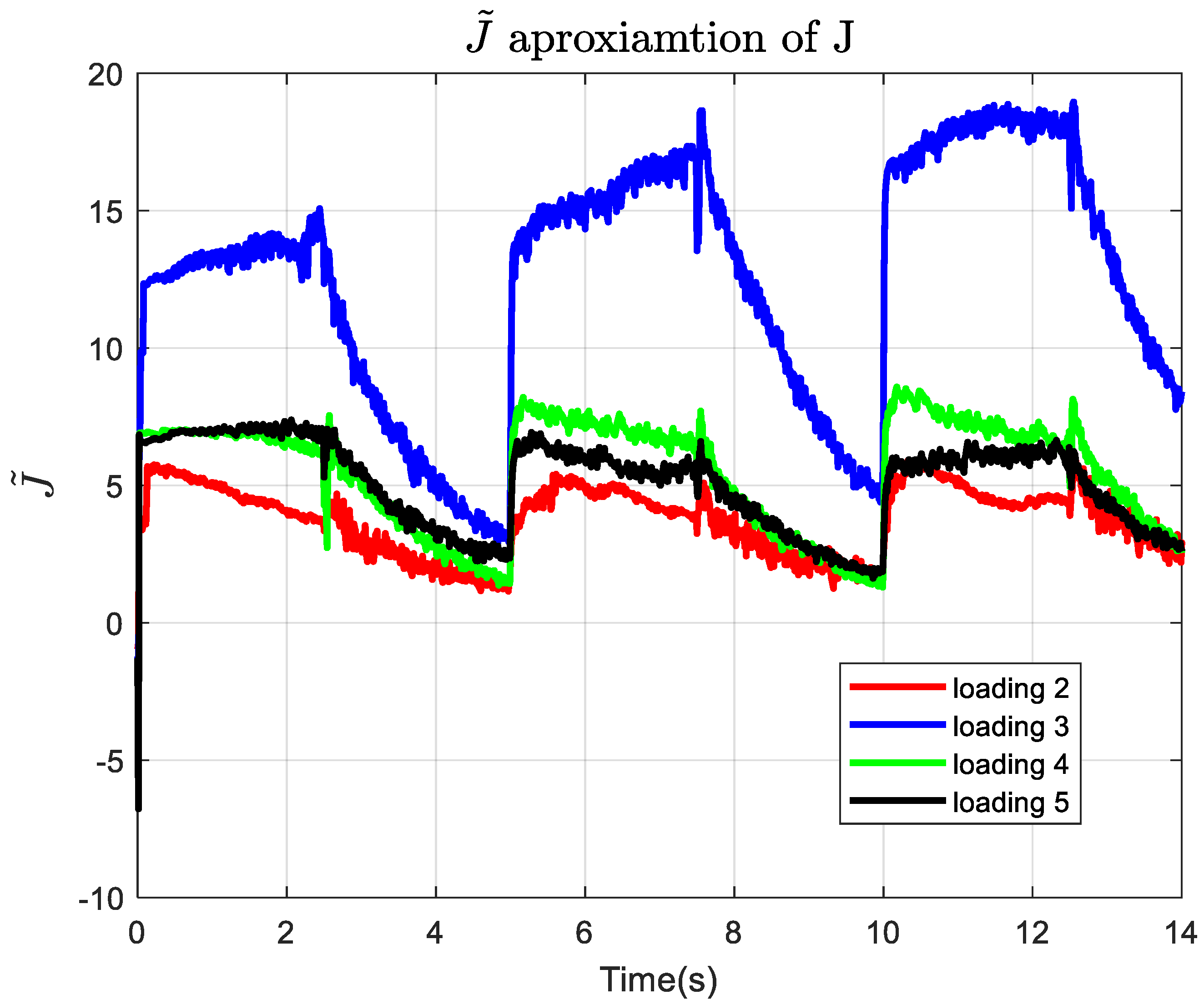
The critic’s approximation (Figure 17) separates the loading regimes clearly: loading 3 remains the highest, around 12–18; loading 4 is intermediate at about 6–8; loading 5 is slightly lower at about 6–7; and loading 2 is the lowest at about 3–5 most of the time. As expected, it is functionally dependent on the control level and tracking error. The trajectories also show the adaptive critic updating online in response to the operating-point changes: each loading case has step-like rises and decays synchronized with the reference changes, which is what one expects from Bellman-error-driven learning as the closed-loop error evolves.

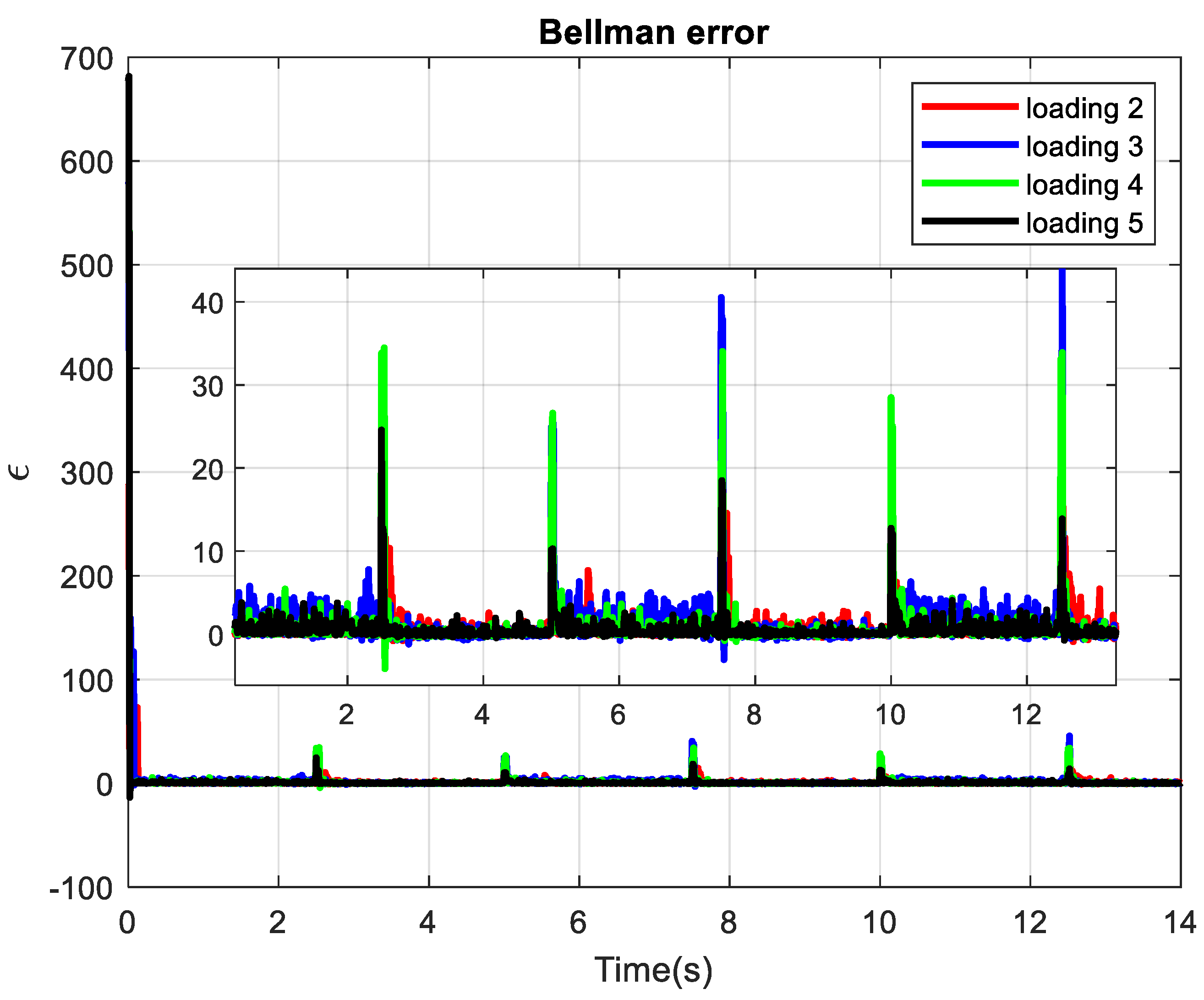
The Bellman error (Figure 18) stays close to zero for most of the run in all four load cases, which is the key adaptive-critic signature of a critic that has largely matched the value recursion.

The transient spikes appear mainly at the reference switching instants, with the largest visible excursions under loading 3 and loading 4, reaching roughly 40–50, while loading 2 and loading 5 have smaller peaks, roughly 10–20. In adaptive dynamic programming terms, this means the critic is repeatedly correcting its value approximation when the operating point changes, then quickly decays the error as learning converges. So, the figure supports convergence of the critic to a near Bellman-consistent solution, and the small steady-state error between switching events indicates stable online learning rather than persistent misfit.

6. Conclusions

This study demonstrates that the proposed PI-based adaptive actor–critic controller can be implemented in real time on an industrial hydraulic test bench and can effectively regulate the displacement volume of an axial-piston pump over a wide range of loading conditions. The experimental results show that the controller maintains a stable closed-loop operation, achieves small tracking errors, and adapts successfully to both fixed loads and load variations, confirming that the model-free design is practical for uncertain nonlinear hydraulic systems. The near-zero Bellman error and bounded critic signals further indicate that the learned policy converges to a consistent value approximation during operation.

A key outcome of the article is the clear performance advantage over conventional PI control and the Lyapunov-based MRAC baseline. Across the reported loading conditions, the proposed PIAC controller achieves the lowest performance index and the shortest settling times in most cases, showing that the PI actor provides an effective structure for fast adaptation while preserving a simple implementation. Compared with the generic actor–critic formulation, the PI-based actor achieves comparable or better transient behavior with a more straightforward control law, which is important for embedded deployment.

The results also highlight the role of the critic in improving robustness under changing operating points. During load transitions, the critic generates a corrective signal that reduces the Bellman residual and helps the controller re-adjust quickly, which explains the observed reduction in oscillation and the improved settling behavior relative to fixed-gain PI control. This makes the proposed approach attractive for hydraulic systems where the plant dynamics vary with pressure and load and where explicit high-fidelity modeling is time- and resource-consuming.

Overall, the article shows that combining a PI actor with an adaptive critic is a strong compromise between implementation complexity and control performance. The method is sufficiently compact for Simulink^®-based code generation and microcontroller deployment; yet, it still captures the benefits of reinforcement-learning-style adaptation in real time. Future work could extend the approach to broader operating envelopes, additional disturbance scenarios, and further hardware simplification while preserving the same stability and convergence properties. The authors acknowledge that the explicit sensitivity analysis of learning rates, forgetting factors, and initial conditions will be beneficial to fully understand the operating envelope of the system, which is also part of the future work. At this point, we can say that the Lyapunov-based stability analysis provides an admissible upper bound on the learning rate. Moreover, the experimental evaluation across several loading conditions and dynamic load variations demonstrates that the selected parameters yield a stable and consistent performance. In addition, the initial conditions are justified in the manuscript as values that ensure a stable closed-loop system before adaptation begins.