Kuramoto Object-Centric Reinforcement Learning for Robotic Manipulation Tasks

Abstract

Model-based reinforcement learning (MBRL) is a promising approach for achieving high sample efficiency in learning control policies. The existing world models in MBRL typically represent the environment’s state as a single global latent vector. However, such representations limit the model’s ability to capture object interactions and reason about individual objects—capabilities that are critical for visual object-oriented tasks—and may lead to lower sample efficiency. To address this limitation, we propose Kuramoto Object-Centric Reinforcement Learning (KORL), a model-based agent that learns an object-centric world model. Our approach introduces a novel Kuramoto Slot Attention for Video (KSAVi) model that integrates Kuramoto oscillatory neurons with the Slot Attention module to robustly extract object representations. We design a world model that leverages these structured object-centric latents and predicts dynamics using graph neural networks, thereby incorporating an inductive bias for modeling object interactions. We evaluate KORL on a suite of visually diverse object-oriented robotic manipulation tasks and demonstrate that our method outperforms object-centric model-free and model-based approaches.

1. Introduction

Automating routine tasks enhances productivity across industries, from defect-based object sorting to automotive welding. Classical continuous control algorithms can achieve this but require meticulous tuning to handle edge cases; unexpected failures may halt production entirely. In contrast, trainable approaches like reinforcement learning (RL) can adapt to diverse real-world scenarios given sufficient training time.

RL has demonstrated success in both synthetic environments [1,2,3] and real-world applications [4,5]. However, studies show that RL performance can benefit, in terms of sample efficiency and generalization, from better representations of the environment states obtained through contrastive learning [6], fusion of state and action information [7], image augmentation and auxiliary reconstruction objectives [8,9], and specialized encoder architectures and pretraining [10].

A promising approach to improving RL representations involves disentanglement: instead of compressing scene information into a single monolithic vector, the information can be decomposed into an array of vectors, each representing distinct components. Slot Attention [11] formalizes this idea by partitioning inputs (e.g., images or videos) into independent slots—interpretable vectors that encode individual scene elements and support scene reconstruction.

The advantage of object-centric representations in RL becomes evident when paired with interaction-aware models (e.g., transformers [12] or GNNs [13]) that aggregate slot information to reason about inter-object relationships. This explicit modeling of interactions improves both policy learning and generalization.

Prior work has applied object-centric representations to both model-free [10,14] and model-based RL [15,16,17]. We focus on the latter, where disentangled representations enable explicit modeling of object interactions—beneficial for both policy and world model learning.

We identify two main questions in object-centric RL: (1) how to obtain object-centric representations and (2) how to use them in an RL algorithm. In this work, addressing the first question, we present a novel object-centric model, Kuramoto Slot Attention for Video, which reliably extracts disentangled object representations across a set of visually diverse tasks. Addressing the second question, we propose a model-based RL algorithm that employs a graph neural network as a world model, enabling it to internally maintain disentangled latent object states.

The main contributions of this work are as follows:

• We introduce the Kuramoto Slot Attention for Video (KSAVi) model, an object-centric encoder that integrates Slot Attention with Kuramoto oscillatory neurons, enabling robust extraction of object representations that are suitable for downstream reinforcement learning with fixed hyperparameters across visually diverse tasks.
• We propose a novel object-centric model-based Kuramoto Object-Centric Reinforcement Learning algorithm (KORL) that combines a pretrained object-centric KSAVi encoder with a graph neural network (GNN) world model to exploit structured object representations for planning.
• Through experiments on visually diverse robotic manipulation tasks, we demonstrate that KORL achieves more robust performance than existing object-centric model-free and model-based RL baselines with fixed hyperparameters.
• We show that KORL exhibits zero-shot generalization under significant changes in scene appearance, while monolithic model-based RL methods fail.
• We provide empirical evidence that KSAVi is more suitable for RL than the state-of-the-art object-centric video model SlotContrast [18] as replacing KSAVi with SlotContrast in KORL reduces performance.

2. Related Work

2.1. Object-Centric Representations for Images

The introduction of the Slot Attention module [11] has spurred the development of numerous methods that retain it as the core mechanism for unsupervised slot extraction while proposing architectural optimizations. For instance, SLATE [19] replaces traditional independent slot reconstruction with a transformer decoder, enabling better image reconstruction and slot composability.DINOSAUR [20] addresses the challenge of real-world image representations by reconstructing frozen DINO [21] features instead of raw pixels. FT-DINOSAUR [22] extends this by enabling encoder fine-tuning: it uses a frozen target encoder to generate stable DINO features for slot reconstruction, while an unfrozen encoder extracts features for Slot Attention, thus preventing model collapse during training.

A separate line of work achieves unsupervised scene decomposition without Slot Attention by partitioning latent vectors into subcomponents representing distinct object attributes (e.g., position, shape, and color). A distinctive feature of such methods is the increased number of vectors used in image reconstruction compared to Slot Attention. Examples include the Deep Latent Particles (DLP) model [23] and SPACE [24].

An notable model in this field is the AKOrN [25] neural network architecture, in which units are high-dimensional Kuramoto oscillatory neurons. This architecture enables synchronization, or “binding”, between neurons, leading to competitive performance in object discovery and reasoning.

2.2. Object-Centric Representations for Videos

While Slot Attention naturally extends to videos [26], handling sequences of images requires ensuring the temporal consistency of slots (i.e., the same object should be bound to the same slot across frames). Recent methods address this by modeling inter-frame dependencies. OCVP [27] introduces masks to capture temporal and positional relationships between slots, while VIDEOSAUR [28] adds a loss term to predict future slot transitions. SlotContrast [18] extends DINOSAUR to video by enforcing object-level temporal consistency through a contrastive loss. SOLV [29] aggregates temporal slot information via a transformer encoder.

2.3. Reinforcement Learning

Reinforcement learning for control is typically divided into model-free and model-based approaches. Model-based methods [3,30,31] build a model of the environment and use it for training and planning. Model-free methods [32,33,34,35] learn directly from data without a world model.

The main advantage of model-based RL is sample efficiency: by learning a dynamics model, agents can generate trajectories without interacting with the real environment. DreamerV3 [3] uses a Recurrent State-Space Model (RSSM) with $32\times 32$ discrete categorical latent codes, training an actor–critic entirely on imagined latent trajectories. It uses a single set of hyperparameters across all tested tasks (both continuous and discrete). MuZero [31] uses a value-equivalent model that predicts only rewards, values, and policies rather than raw observations. It employs Monte Carlo Tree Search in latent space and masters Go, chess, shogi, and 57 Atari [36] games. Its descendants have been particularly successful in discrete domains: EfficientZero [37] adds self-supervised consistency losses to achieve a 194% mean human-normalized score on the Atari 100 k benchmark. EfficientZero V2 [38] extends this approach to both discrete and continuous control using sampling-based Gumbel search but still demonstrates stronger performance on discrete control tasks. DIAMOND [39] replaces the discrete tokenizer with a diffusion world model. TD-MPC2 [40] is designed for continuous action spaces and takes a different approach: it uses decoder-free latent dynamics with Model Predictive Path Integral (MPPI) planning over short horizons, combined with a terminal value function for long-term return estimation. It outperforms DreamerV3 on 104 continuous control tasks using a single set of hyperparameters.

Model-free methods are widely used in practice, especially when environments are complex or simulation is cheap enough to run billions of steps. Off-policy algorithms can reuse past experience via replay buffers, achieving much higher data efficiency at the cost of potential instability. Among the off-policy methods for continuous control, TD3 [41] is often a top performer on robotic fetch tasks and standard MuJoCo [42] locomotion benchmarks. It uses clipped double Q-learning, delayed policy updates, and target policy smoothing. SAC [35] is trained using a maximum-entropy objective, which maximizes both return and policy entropy. It provides robust exploration and more stable training. SAC-AE [43], DrQ [8], and DrQ-v2 [9] demonstrate the importance of data augmentation and auxiliary reconstruction objectives for improving the performance of off-policy algorithms in image-based continuous tasks. A large body of recent work focuses on introducing diffusion-based policies into off-policy RL [44]. For example, the recently proposed SDAC [45] consistently improves the performance of SAC by integrating a diffusion policy.

For discrete control tasks, the off-policy Agent57 [1] remains a strong baseline for the Atari benchmark. It was the first deep RL agent to outperform human-level performance across all 57 games in the set. It combines off-policy learning with episodic memory to address long-term credit assignment and exploration. BBF [46] is the first model-free agent to achieve superhuman performance on the Atari 100 k benchmark. It uses a larger convolutional encoder than Agent57, dynamic schedules for n-step learning and the discount factor, a higher replay ratio, and other improvements.

On-policy algorithms update the policy using only the most recent data, generally yielding stable learning but poor sample efficiency. PPO [33] is a dominant on-policy algorithm. Its clipped surrogate objective prevents catastrophic policy updates while requiring only first-order optimization compared to TRPO [47]. It works for both discrete and continuous action spaces, parallelizes across thousands of environments, and is known for its training stability compared to off-policy methods. The combination of PPO with highly parallelized GPU-accelerated simulation has become the industry-standard pipeline for robot learning [48,49]. Recent work focuses on introducing diffusion policies into the on-policy setting [50,51] and modifying the PPO objective [52].

2.4. Object-Centric Reinforcement Learning

Object-centric models enhance RL in two ways. In model-free RL, object-centric models can be employed as (1) frozen pretrained feature extractors (analogous to CNNs [53] in image-based environments), an approach validated through large-scale studies [10]; (2) via representation distillation, exemplified by OCARL [54], which leverages SPACE’s [24] object discovery capabilities to cluster detected objects and trains a CNN encoder to predict these clusters. The CNN encoder is then used as a feature extractor for the actor and critic; (3) through end-to-end training [14], although this method may produce object slots that inconsistently correspond to meaningful entities.

Object-centric representations are also utilized in goal-conditioned RL algorithms. SMORL [55] employs a patch-based image representation model SCALOR [56] and a goal-conditioned attention policy. A key limitation of SMORL is its assumption that multi-object tasks can be addressed sequentially and independently, ignoring potential interactions between objects. A more recent goal-conditioned approach, ECRL [57], uses a DLP encoder to represent objects and transformers for the actor and critic models. These components are trained using the TD3 algorithm [41] in object manipulation tasks, incorporating an intrinsic reward based on the distance between features of objects in the current and goal images. This approach requires supervision during training to learn a model that differentiates objects of interest from irrelevant particles. The model is used for computing the intrinsic reward.

In model-based RL, the concurrent approach SOLD [16] employs a pretrained SAVi model [58] to extract object-centric representations, integrating them into world models to enable long-horizon prediction on specific tasks. SOLD is evaluated on a set of tasks that exhibit diverse dynamics but are visually similar. Another line of research explores the use of supervision to extract object-centric representations. FOCUS [17] incorporates an online-learning object-centric encoder that requires segmentation masks during training. These masks are either provided by the simulator (supervised mode) or generated using the Segment Anything Model [59] with a single labeled sample (weak supervision). FOCUS also introduces an intrinsic reward that encourages interaction with objects. OC-STORM [60] utilizes CUTIE’s [61] object memory representations after few-shot supervised pretraining on a dataset of ground-truth object segmentations. A notable feature of OC-STORM is its ability to leverage both monolithic and object-centric representations. Both FOCUS and OC-STORM operate in visually complex environments and rely on access to labeled data.

Object-centric approaches are also used in environments providing vector (non-image) state representations. DAFT-RL [62] is a model-based method where the state is factored into objects and their attributes (e.g., physical and visual properties). It learns several networks involving three graphs: one models the relationship between object attributes, agent actions, and rewards; the second captures object–object interactions; and the third handles agent–object interactions and forward dynamics. However, it requires environments where single-object episodes can be easily generated. The goal-conditioned model-based algorithm SRICS [63] accounts for object–object interactions by using a graph neural network (GNN) as a transition model and learns a policy that moves the objects one by one.

Our approach, KORL, requires no supervision and is designed for image-based RL control tasks (non-goal-conditioned setting).

3. Materials and Methods

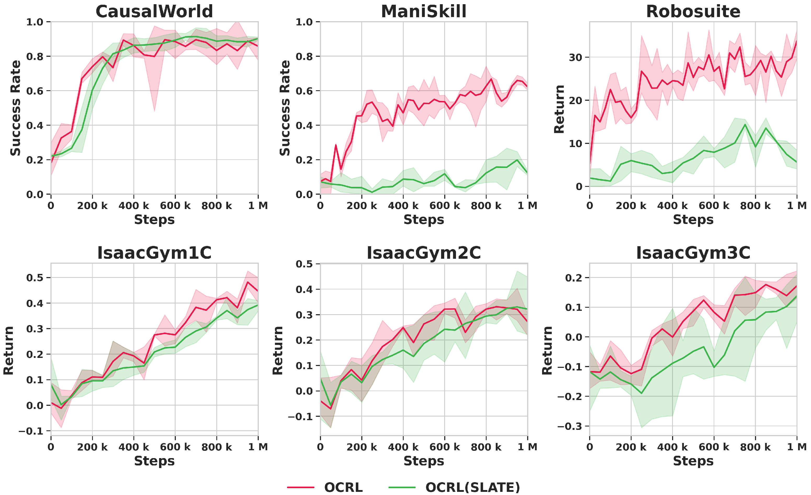
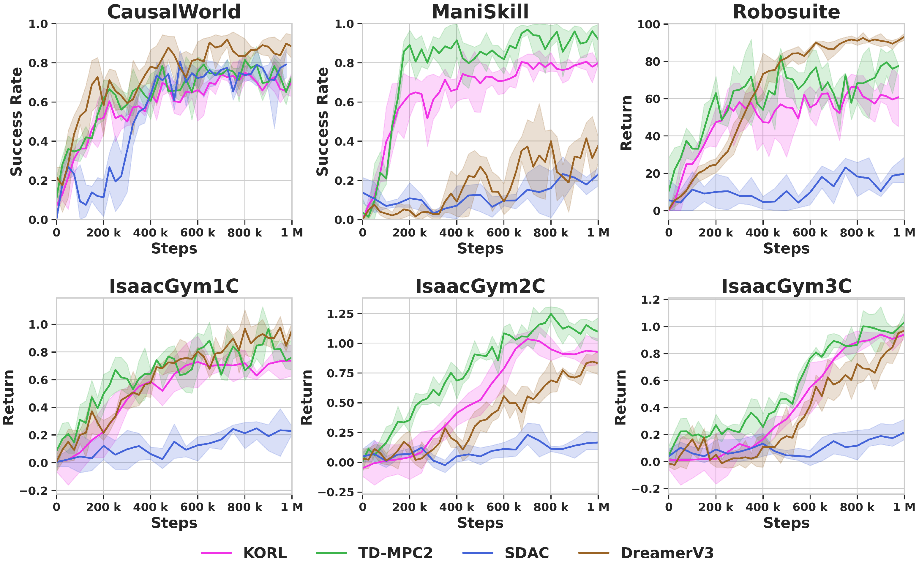
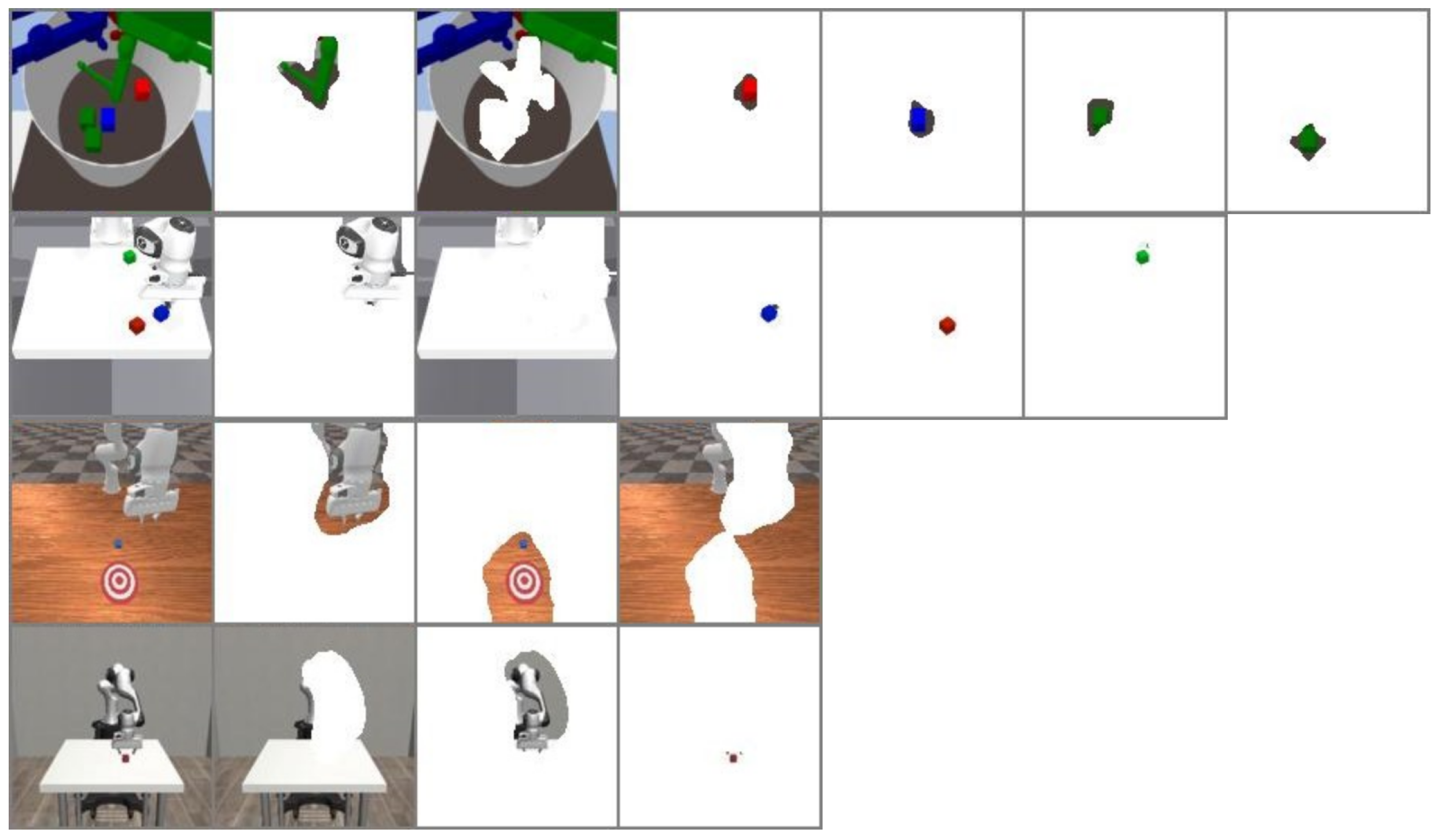
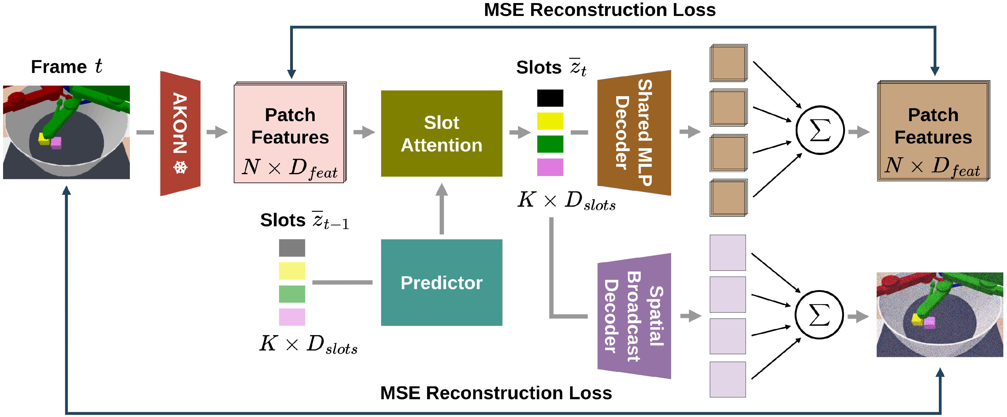
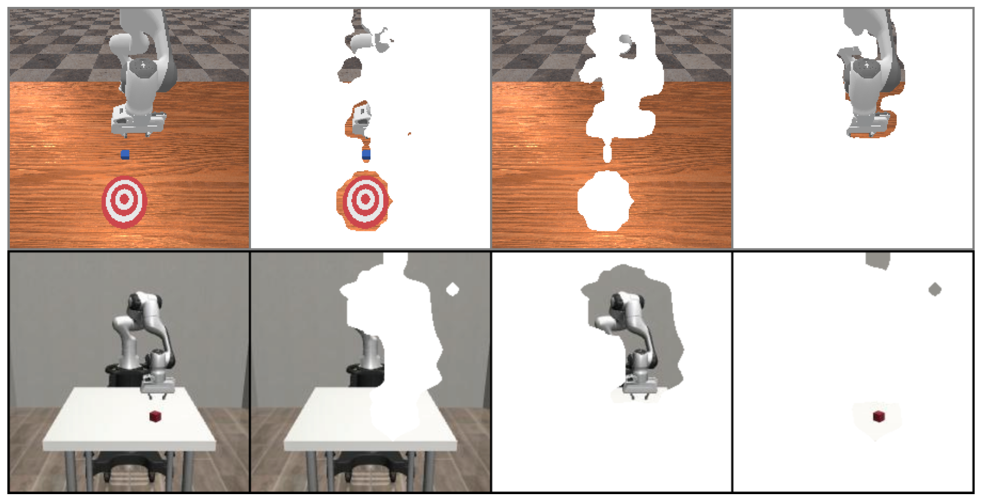
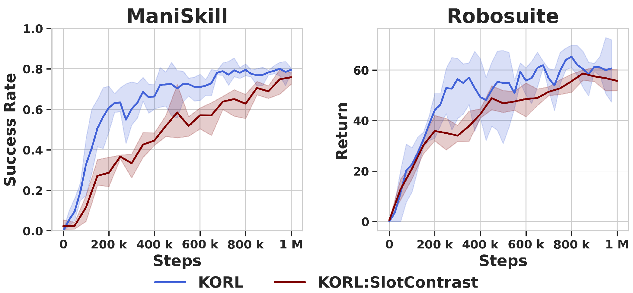
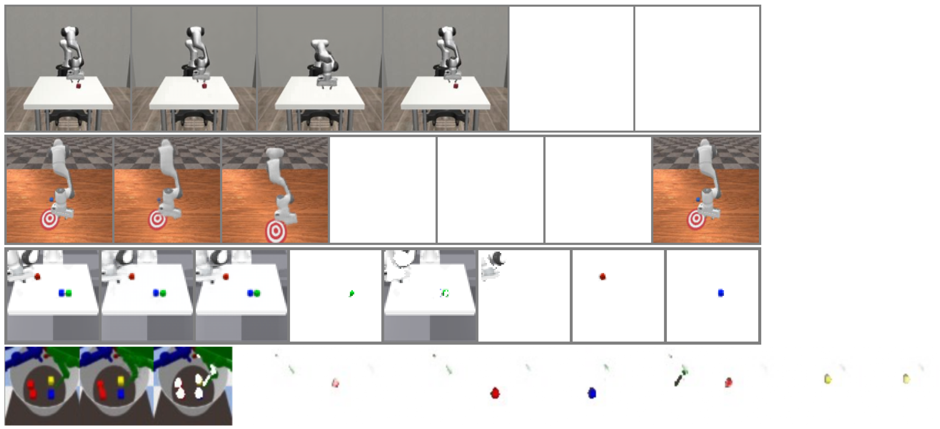
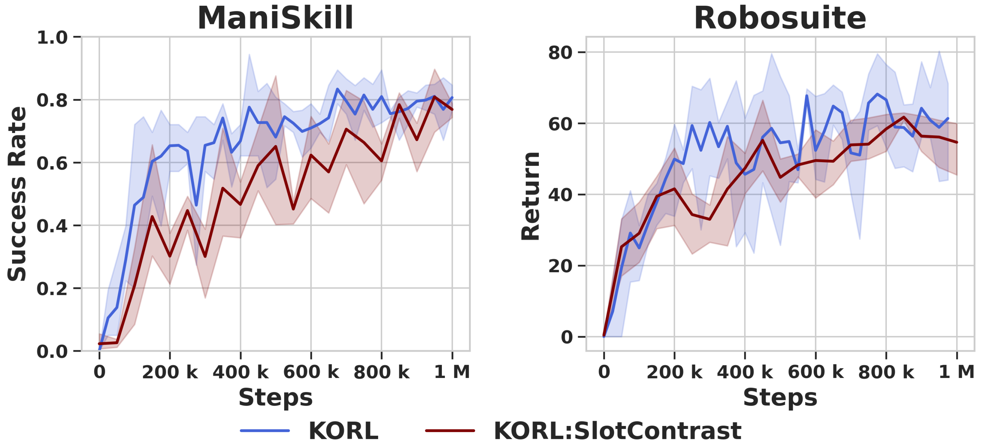
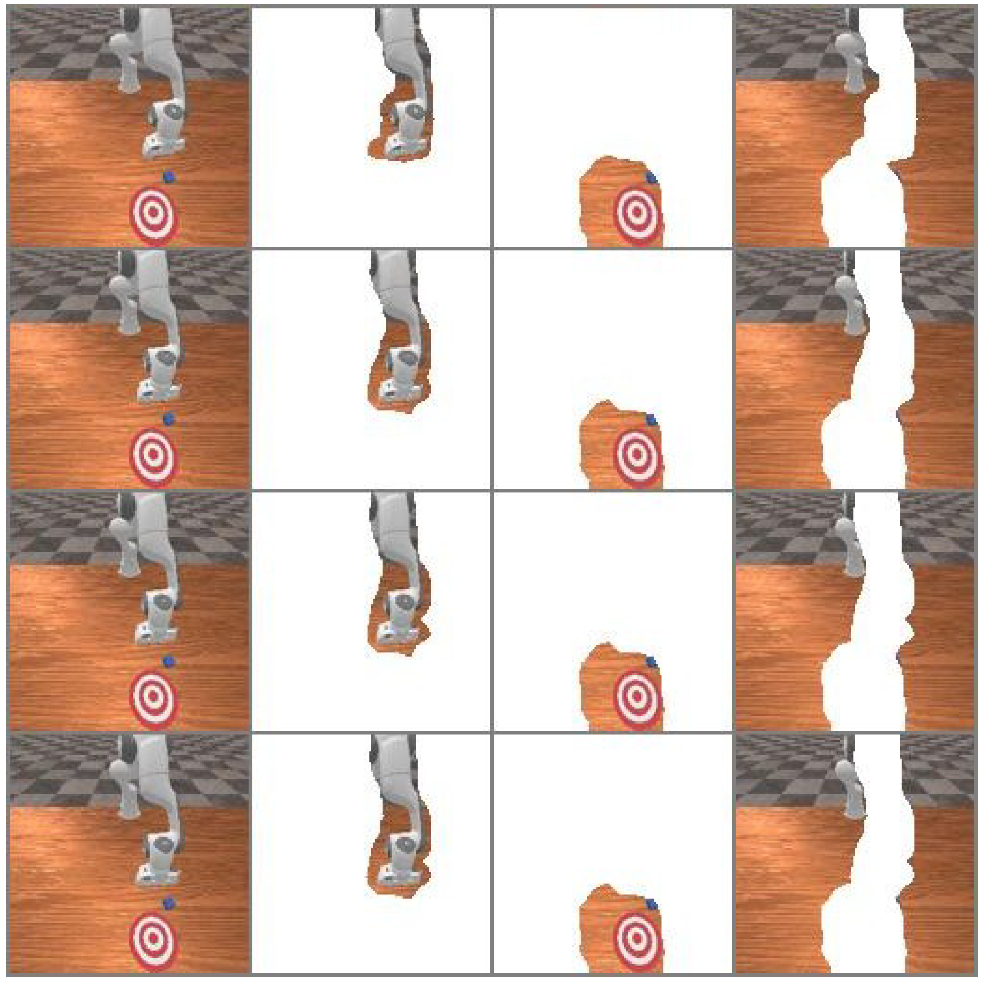
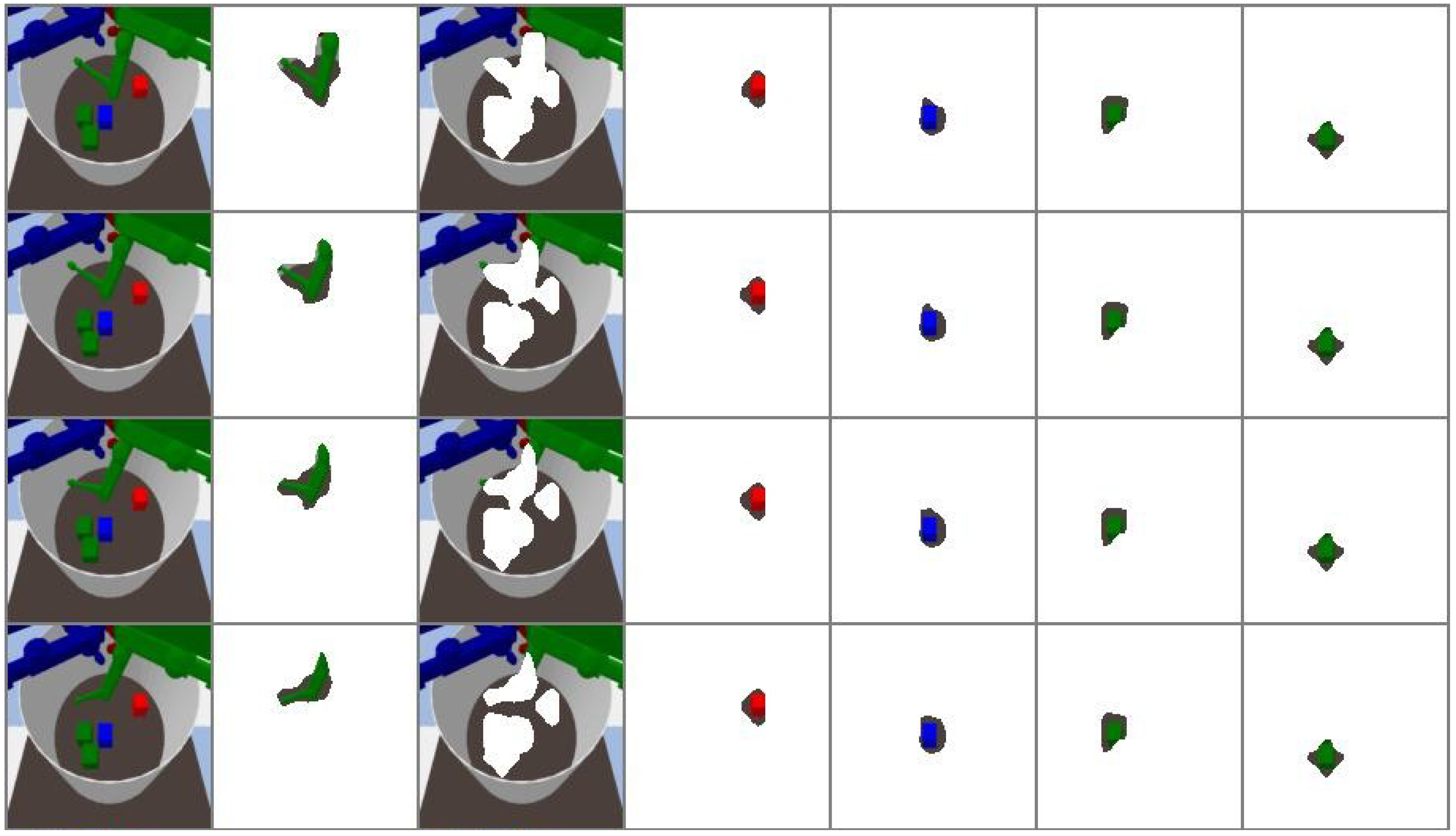
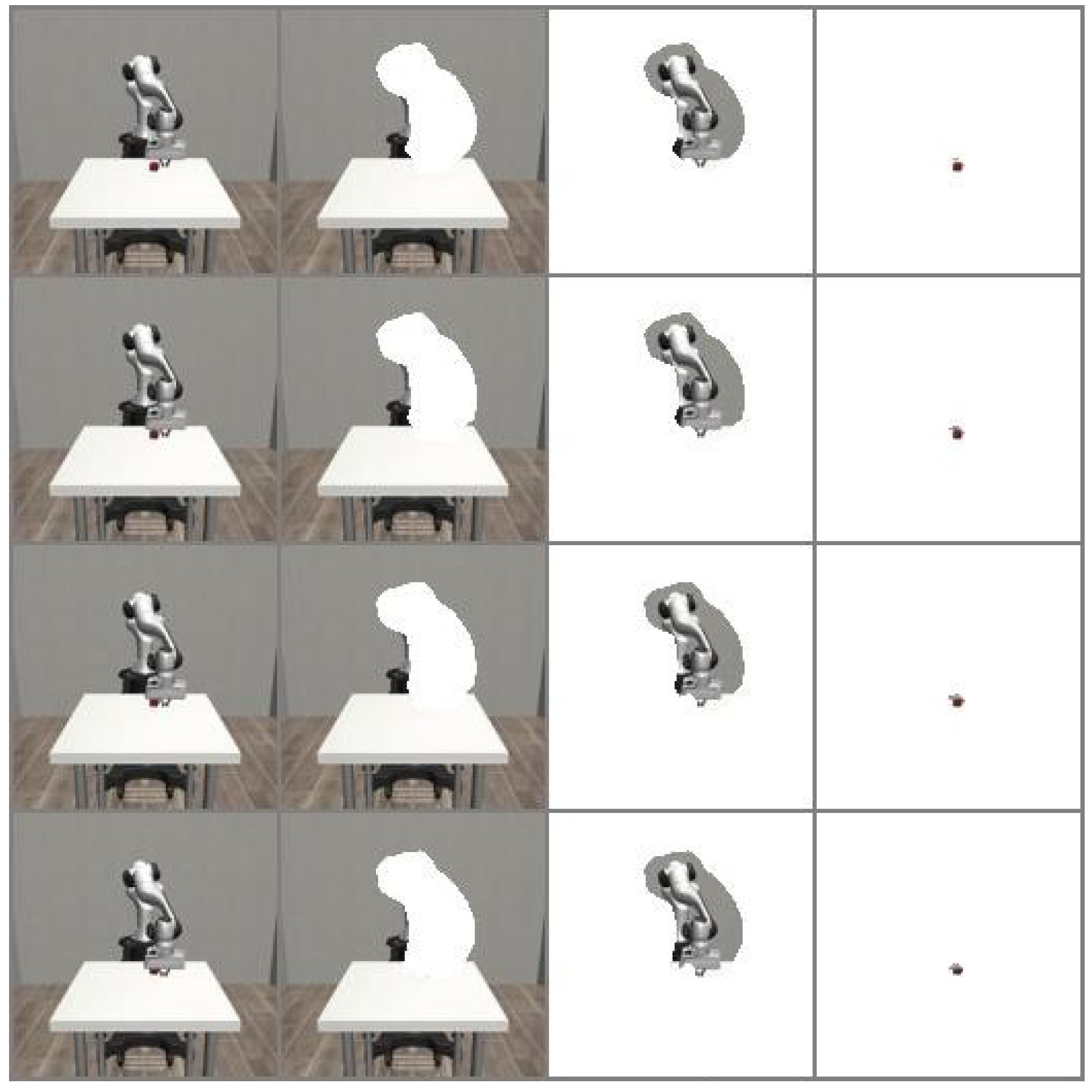
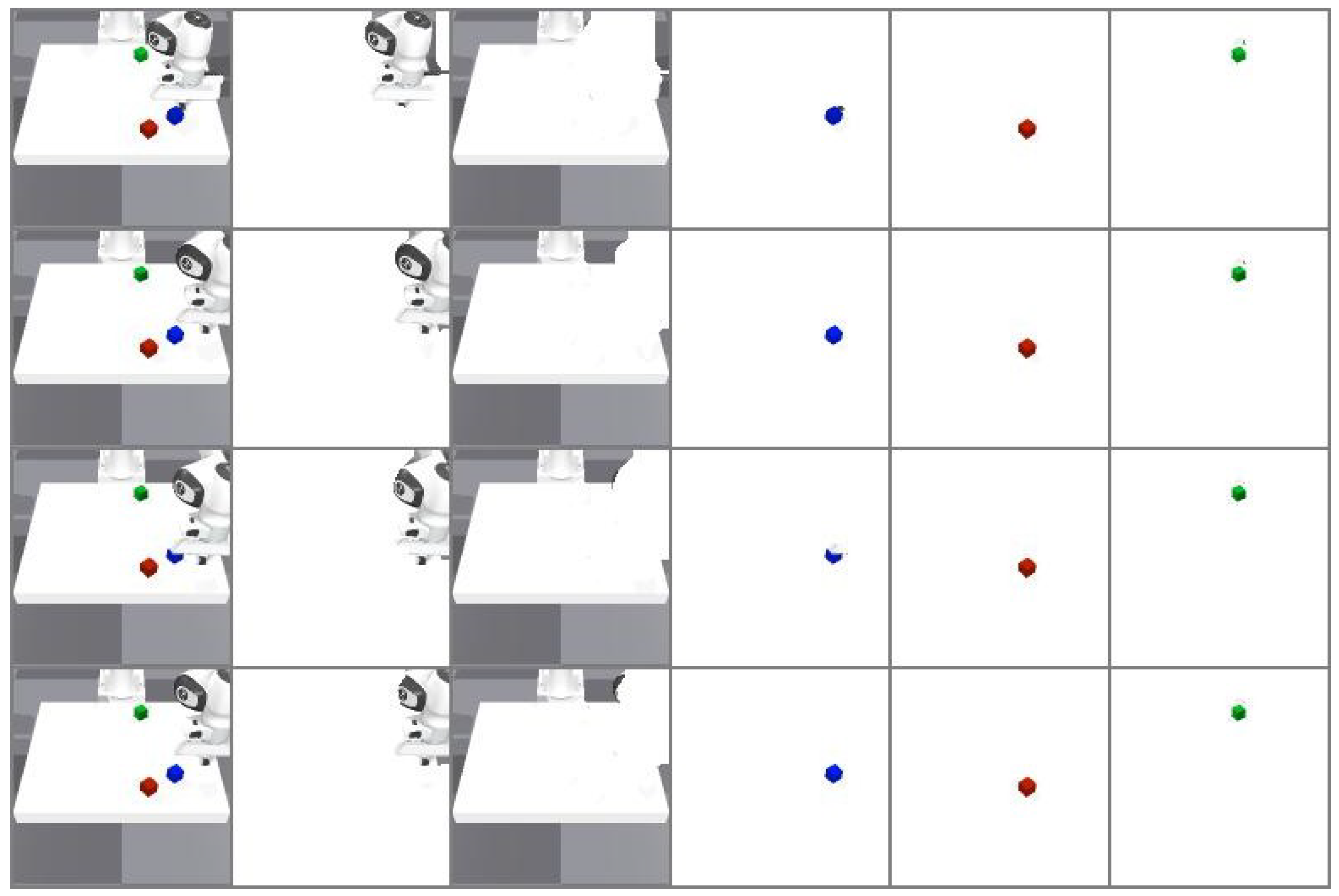
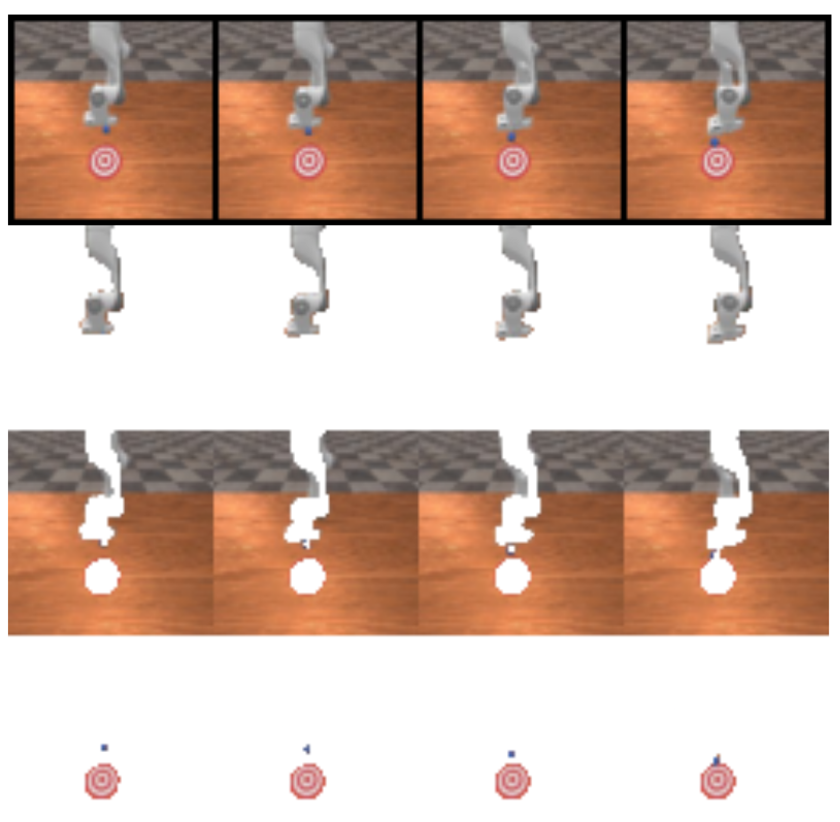
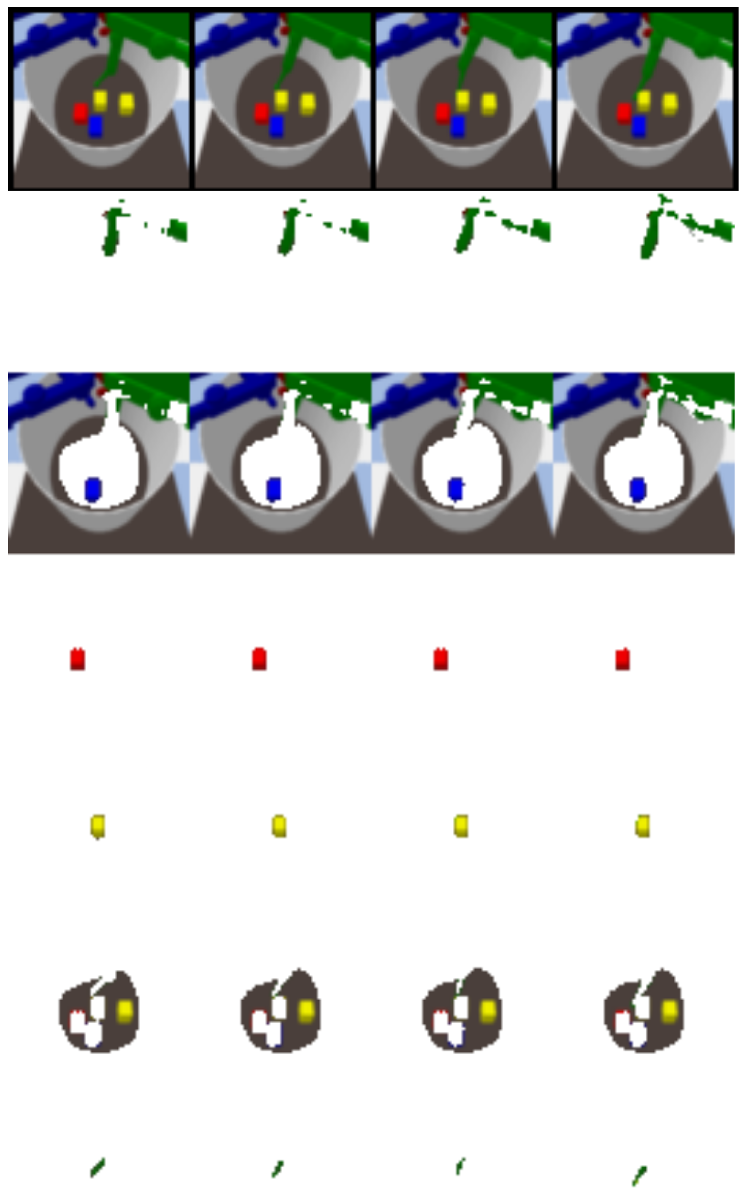
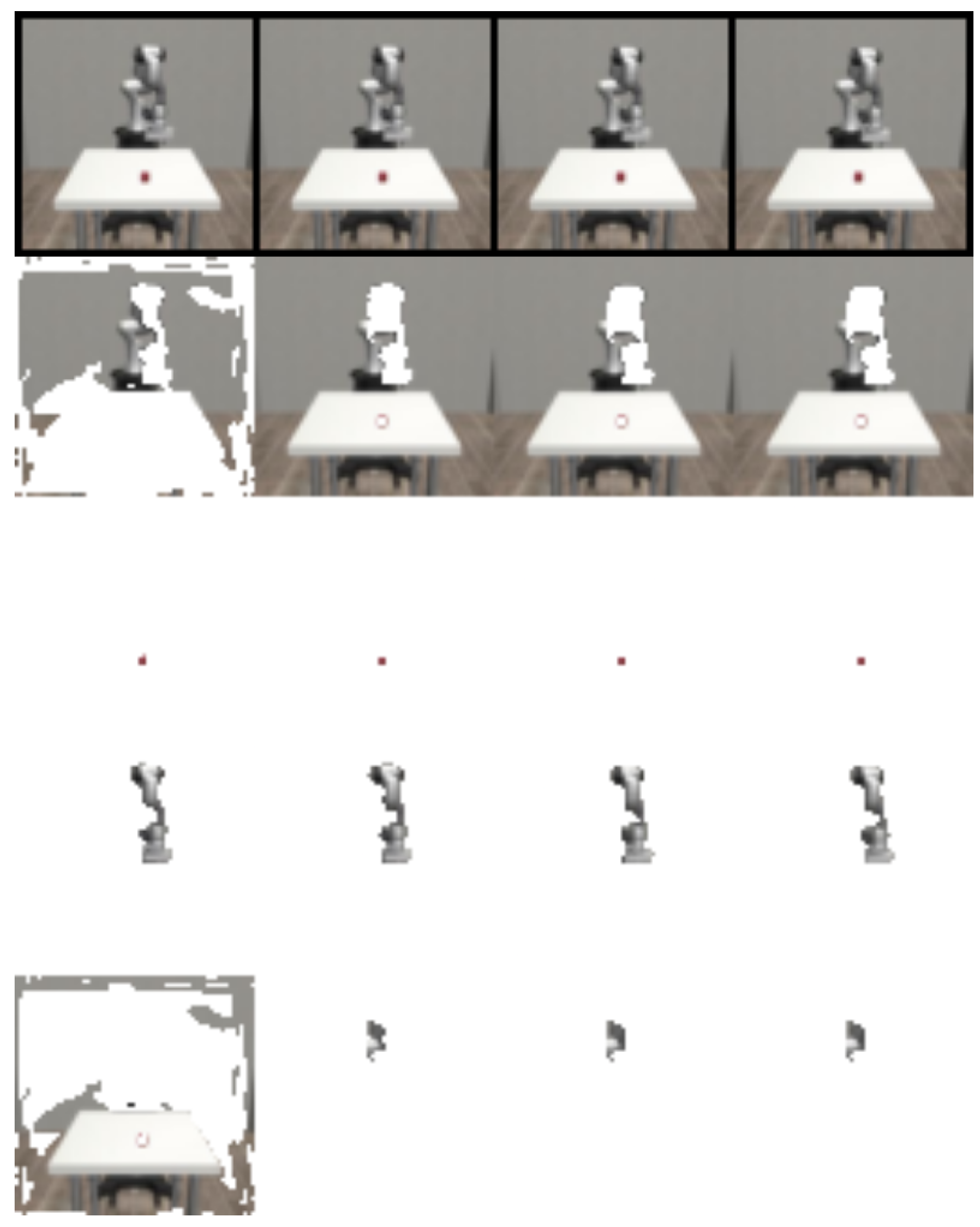
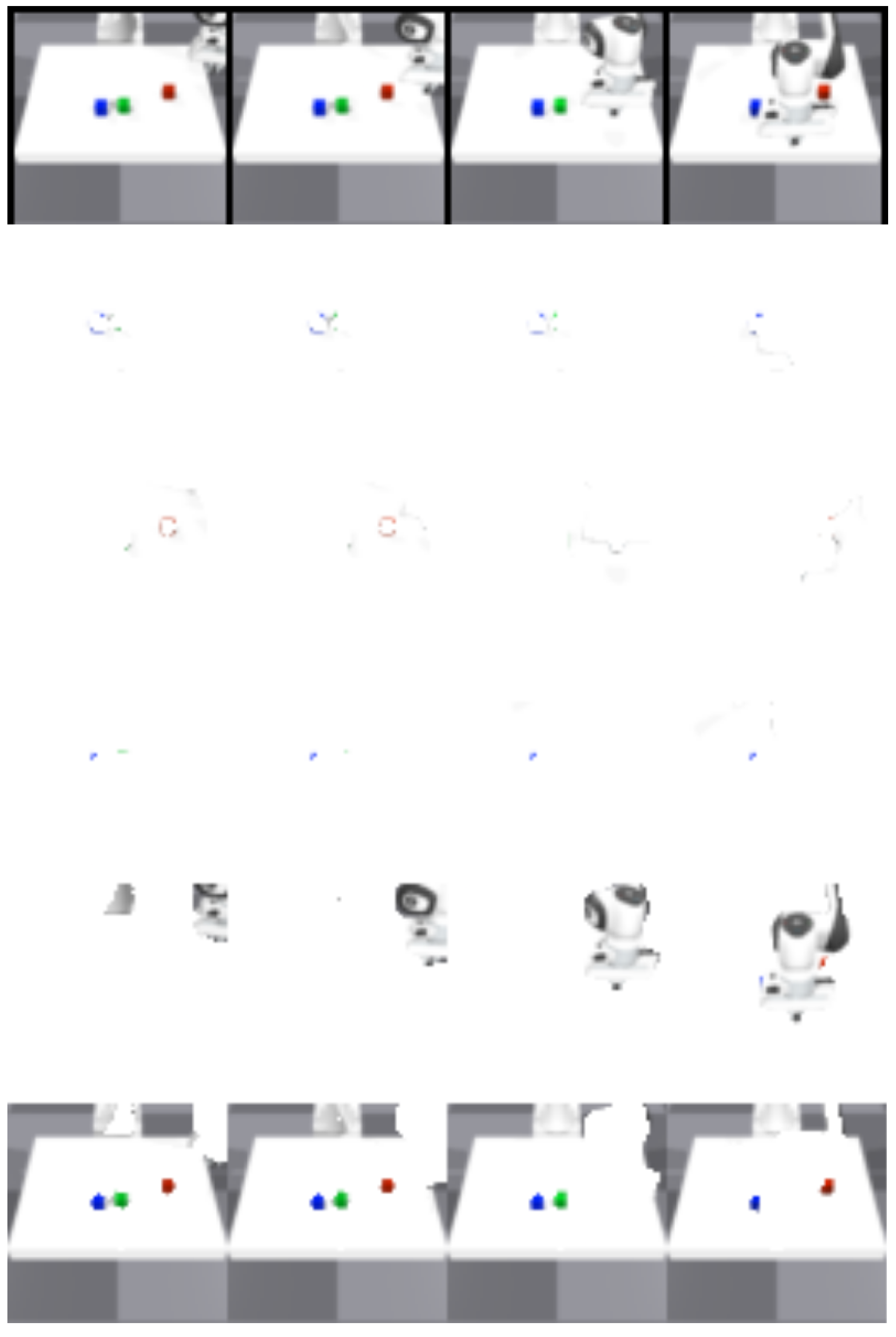
This section describes our Kuramoto Object-Centric Reinforcement Learning (KORL) algorithm. KORL builds on Temporal-Difference Model Predictive Control for policy learning and leverages our Kuramoto Slot Attention for Video (KSAVi) model as an object-centric encoder. We first provide brief introductions to Temporal-Difference Model Predictive Control (Section 3.1), Slot Attention (Section 3.2), and Artificial Kuramoto Oscillatory Neurons (Section 3.3), followed by descriptions of KSAVi (Section 3.4), KORL (Section 3.5), and the experimental setup (Section 3.6).

3.1. Temporal-Difference Model Predictive Control

Continuous control problems can be defined as a Markov decision process (MDP) [64] represented by $M=(S,A,\rho ,{\rho }_0,r,\gamma )$, with state space S, action space A, transition function $\rho (s^{\prime },s,a)$, initial state distribution ${\rho }_0$, reward function $r(s,a)$, and discount factor $\gamma \in [0,1]$. The objective of the agent is to learn a policy $\pi :S\to A$ that maximizes discounted cumulative reward:

$$J\left(\pi \right)={\mathbb{E}}_{\tau }\left[\sum _{t=0}^T{\gamma }^{t}r(s_t,a_t)\right],$$

(1)

where $\tau$ is a trajectory sampled by executing $\pi$.

Model-based RL leverages the internal structure of the MDP by learning a dynamics model, which approximates the transition function $d\approx \rho$, and a reward model, which approximates the reward function $\widehat{r}\approx r$. These two components enable planning future actions and estimating their outcomes rather than relying solely on a value function estimator. A refined closed-loop control policy can be obtained through local trajectory optimization methods such as Model Predictive Path Integral (MPPI) [65]. Action sequences of length H are sampled and evaluated by rolling out latent trajectories. At each step, parameters ${\mu }^{\ast }$ and ${\sigma }^{\ast }$ of a multivariate Gaussian are computed to maximize the expected return G:

$$\begin{array}{cc}\hfill {\mu }^{\ast },{\sigma }^{\ast }& =\underset{\mu ,\sigma }{argmax}{\mathbb{E}}_{(a_t,\dots ,a_{t+H})\sim \mathcal{N}(\mu ,{\sigma }^2)}\left[G\left(s_t\right)\right],\hfill \end{array}$$

(2)

$$\begin{array}{cc}\hfill G\left(s_t\right)& =\sum _{h=1}^{H-1}{\gamma }^{h}r(z_h,a_h)+{\gamma }^H\widehat{V}\left(z_{t+H}\right).\hfill \end{array}$$

(3)

$\mu ,\sigma \in {\mathbb{R}}^{H\times m}$, where $m=dimA$. After solving the problem (Equation (2)), only the first action $a_t\sim \mathcal{N}({\mu }_t^{\ast },{{\sigma }_t^{\ast }}^2)$ is executed. The optimization problem is then re-solved at the next time step $t+1$. This iterative procedure effectively yields a H-step look-ahead policy, which leverages both the planner and the value function $\widehat{V}$.

Combining planning and temporal-difference learning has proven to be an effective strategy for reducing the planning horizon and improving data efficiency. A widely adopted pipeline, proposed in TD-MPC2 [40], learns a world model and performs planning in latent space. It uses an encoding function that maps the state to a latent representation $z_t=h\left(s_t\right)$. The following components are learned in latent space: latent dynamics $z_{t+1}=d_{\theta }(z_t,a_t)$, reward ${\widehat{r}}_t=R_{\theta }(z_t,a_t)$, policy ${\widehat{a}}_t={\pi }_{\theta }\left(z_t\right)$, and state–action value function ${\widehat{q}}_t=Q_{\theta }(z_t,a_t)\approx Q^{{\pi }_{\theta }}(z_t,a_t)$. The components $h_{\theta }$, $d_{\theta }$, $R_{\theta }$, and $Q_{\theta }$ are jointly trained through the following loss:

$$\begin{array}{cc}\hfill L\left(\theta \right)& ={\mathbb{E}}_{(s_t,a_t,r_t,s_{t+1})\sim D}\left[L_d+L_r+L_q\right],\hfill \end{array}$$

(4)

$$\begin{array}{cc}\hfill L_d& =\sum _{t=0}^H{\lambda }^t{\parallel d(z_t,a_t)-\mathtt{sg}\left(h\left(s_{t+1}\right)\right)\parallel }_2^2,\hfill \end{array}$$

(5)

$$\begin{array}{cc}\hfill L_r& =\sum _{t=0}^H{\lambda }^{t}CE({\widehat{r}}_t,r_t),\hfill \end{array}$$

(6)

$$\begin{array}{cc}\hfill L_q& =\sum _{t=0}^H{\lambda }^{t}CE({\widehat{q}}_t,q_t).\hfill \end{array}$$

(7)

where D is a replay buffer; coefficient $\lambda \in [0,1]$ helps the model components to focus more on short-term horizons. Learning of $R_{\theta }$ and $Q_{\theta }$ is formulated as discrete regression problems, with cross-entropy ($CE$) as the loss function. Target $q_t$ is generated by bootstrapping policy ${\pi }_{\theta }$ using the target network $Q_{\theta }^{-}$: $q_t=r_t+\gamma Q_{\theta }^{-}(z_{t+1},{\pi }_{\theta }\left(z_{t+1}\right))$. $\mathtt{sg}$ is a stop-gradient operator.

${\pi }_{\theta }$ is a stochastic Gaussian policy trained with the maximum-Q objective in a model-free manner:

$$L_{\pi }\left(\theta \right)=\underset{{(s_t,a_t)}_{0:H}\sim D}{\mathbb{E}}\left[\sum _{t=0}^H{\lambda }^t\left(\alpha Q_{\theta }(z_t,{\pi }_{\theta }\left(z_t\right))+{\beta }_H\mathcal{H}\left({\pi }_{\theta }(·|z_t)\right)\right)\right],$$

(8)

where $\mathcal{H}$ denotes the policy entropy, ${\beta }_H$ is a constant balancing coefficient, and $\alpha$ is adjusted online using moving statistics. ${\pi }_{\theta }$ is used to select an action at the final state of the sample trajectory, resulting in value estimation as $\widehat{V}\left(z_{t+H}\right)={\mathbb{E}}_{a_{t+H}\sim {\pi }_{\theta }\left(z_{t+H}\right)}\left[Q_{\theta }(z_{t+H},a_{t+H})\right]$, which is appended to the sampled trajectories in (Equation (2)).

TD-MPC2 is an RL method that employs learning-based MPC. Recent methods in this category use sampling-based latent MPPI for legged locomotion [66] and differentiable MPC as a policy for controlling a quadrotor unmanned aerial vehicle [67]. Another category of control methods applies classical control-theoretic MPC in robotics. This includes nonlinear MPC applied for legged locomotion [68], tube-based MPC applied to robotic manipulators [69], and Linear Parameter Varying control for nonholonomic mobile robots [70]. Classical MPC provides formal guarantees and well-defined structure, whereas learning-based MPC offers greater data-driven flexibility and removes the need for an accurate analytical model, which is particularly important in tasks where robots operate directly from raw visual observations.

3.2. Slot Attention

Slot Attention module [11] learns object-centric representations in an unsupervised manner. Given an input image $\mathbf{o}\in {\mathbb{R}}^{H\times W\times 3}$, a convolutional [11] or transformer [20] encoder produces a set of feature vectors

$$\mathbf{f}=\{{\mathbf{f}}_1,\dots ,{\mathbf{f}}_N\},{\mathbf{f}}_i\in {\mathbb{R}}^D,$$

(9)

where $N=H^{\prime }{W}^{\prime }$ is the spatial resolution of the feature map. Positional embeddings are added to preserve spatial information. Slot Attention maintains K latent vectors, or slots, $\overline{\mathbf{s}}=\{{\mathbf{s}}_1,\dots ,{\mathbf{s}}_K\}$ with ${\mathbf{s}}_k\in {\mathbb{R}}^{D_{slot}}$. At each forward pass, slots are initialized either from a Gaussian distribution with learned mean and variance or from K learnable vectors. Slots iteratively attend to features through T rounds of competitive attention.

Let keys, values, and queries be

$${\mathbf{k}}_i=W_k{\mathbf{f}}_i,{\mathbf{v}}_i=W_v{\mathbf{f}}_i,{\mathbf{q}}_k=W_q{\mathbf{s}}_k.$$

(10)

Attention weights are computed across slots

$$a_{ik}={\displaystyle \frac{exp({\mathbf{q}}_k^{\top }{\mathbf{k}}_i/\sqrt{D})}{{\sum }_{j}exp({\mathbf{q}}_j^{\top }{\mathbf{k}}_i/\sqrt{D})}}$$

(11)

and each slot aggregates features as

$${\mathbf{u}}_k=\sum _{i=1}^N{a}_{ik}{\mathbf{v}}_i.$$

(12)

Slots are updated using a recurrent update with a gated recurrent unit (GRU) and a multilayer perceptron (MLP):

$${\mathbf{s}}_k\leftarrow \mathtt{GRU}({\mathbf{s}}_k,{\mathbf{u}}_k),{\mathbf{s}}_k\leftarrow {\mathbf{s}}_k+\mathtt{MLP}\left(\mathtt{LayerNorm}\left({\mathbf{s}}_k\right)\right).$$

(13)

For unsupervised object discovery, each slot is decoded independently via a decoder to produce a reconstruction ${\widehat{\mathbf{x}}}_k$ and a mask ${\alpha }_k$. The masks are normalized across the slot axis via a softmax function. Typical decoders are a spatial broadcast decoder [11] (for reconstructing the input image) or an MLP decoder [20] (for reconstructing the input features). The final reconstruction is

$$\widehat{\mathbf{x}}=\sum _{k=1}^K{\alpha }_k\odot {\widehat{\mathbf{x}}}_k,\sum _{k=1}^K{\alpha }_k=\mathbf{1}.$$

(14)

The model is trained end-to-end using a reconstruction loss:

$${\mathcal{L}}_{\mathrm{rec}}={\parallel \mathbf{x}-\widehat{\mathbf{x}}\parallel }_2^2,$$

(15)

where $\mathbf{x}\leftarrow \mathbf{o}$ if the decoder reconstructs the input image $\mathbf{o}$, or $\mathbf{x}\leftarrow \mathbf{F}$ if the decoder reconstructs the input features $\mathbf{F}$. Independent decoding of slots and slot competition induced by softmax normalization encourage the slots to represent distinct objects in the scene without supervision.

3.3. Artificial Kuramoto Oscillatory Neurons

Artificial Kuramoto Oscillatory Neurons (AKOrNs) [25] replace conventional static activation units with dynamical oscillatory states. Instead of representing neuron activity as a scalar activation, each neuron is modeled as an oscillator whose state evolves over time through interactions with other oscillators. In AKOrN, the state of neuron i is represented by a unit vector

$$x_i\in {\mathbb{R}}^d,\parallel x_i\parallel =1,$$

(16)

which lies on the surface of a d-dimensional hypersphere. This vector can be interpreted as a generalized phase representation of the oscillator. The unit-norm constraint ensures that the neuron state evolves through rotations rather than magnitude changes.

The temporal evolution of oscillatory neurons is described using a generalized Kuramoto-type dynamical system, which is approximated using a discretized update rule. Let $x_i^{\left(t\right)}$ denote the oscillator state at iteration t. The system is iterated for T steps according to

$$x_i^{(t+1)}=\mathrm{Normalize}\left({\Omega }_i{x}_i^{\left(t\right)}+c_i+\sum _j{J}_{ij}{x}_j^{\left(t\right)}\right),$$

(17)

where ${\Omega }_i\in {\mathbb{R}}^{d\times d}$ is a skew-symmetric matrix describing the intrinsic oscillatory dynamics of neuron i. It induces intrinsic rotation of the oscillator. $J_{ij}$ denotes the connectivity or coupling strength between oscillators i and j. It drives synchronization between coupled neurons. $c_i$ is an external input term. Normalization ensures that the unit-norm constraint is preserved. Oscillators that receive similar inputs and share strong coupling tend to align their states on the hypersphere. Unrolling these updates yields a recurrent computation that allows oscillators to iteratively exchange information.

In applications to image-processing neural network architectures, oscillatory neurons are typically associated with spatial tokens or feature vectors extracted from an image, and the connectivity matrix J determines how tokens interact. J is typically implemented using convolutional or attention-based architectures.

After T iterations, the resulting states $x_i^{\left(T\right)}$ encode the outcome of the synchronization process. A readout module is used to convert these oscillator states into suitable representations for downstream objectives:

$$z_i={\mathtt{MLP}}_{\psi }\left(x_i^{\left(T\right)}\right),$$

(18)

where ${\mathrm{MLP}}_{\psi }(·)$ is a learnable projection function implemented as a multilayer perceptron (MLP). Because synchronized oscillators tend to produce similar states $x_i^{\left(T\right)}$, the readout embeddings $z_i$ inherit this grouping structure. Consequently, tokens that belong to the same object in the image tend to produce similar embeddings, while tokens belonging to different objects remain separated.

When AKOrN is trained on a dataset of images for the task of unsupervised object discovery, each image is divided into patches. $c_i$ is initialized using the patch features obtained from a convolutional encoder. Each $x_i$ is initialized as a random oscillator sampled from the uniform distribution on the sphere. The model is trained end-to-end using a SimCLR-style [71] contrastive objective applied to the readout embeddings. The input images are augmented by random resizing, cropping, and color jittering. The combination of oscillatory synchronization and contrastive learning encourages the model to learn consistent grouping of visual elements. Tokens corresponding to the same object receive similar inputs and interactions, which promotes synchronization of their oscillator states. Through the readout projection and contrastive objective, these synchronized states produce embeddings that cluster together. As a result, objects emerge as coherent groups of synchronized oscillators, enabling unsupervised discovery of object structure without explicit supervision.

3.4. Kuramoto Slot Attention for Video

We propose Kuramoto Slot Attention for Video (KSAVi), a novel unsupervised object-centric model that integrates AKOrN [25], an encoder based on Kuramoto oscillator neurons, with a Slot Attention module [11]. While AKOrN encoders can bind object features effectively, they do not produce compact vector representations of extracted objects that can serve as abstract object states for downstream tasks such as reinforcement learning. To address this limitation, we train a Slot Attention module on features extracted from images by the AKOrN encoder. The Slot Attention module groups these features into a set of latent vectors—called slots—which we use as latent object states in our RL algorithm KORL.

The training pipeline for KSAVi is inspired by the SAVi [26] and DINOSAUR [20] approaches and proceeds as follows: (1) collect a dataset of episodes in the environment using a uniform random policy; (2) train the AKOrN encoder on the collected images; (3) train the Slot Attention module on the collected data, treating sequences of episode images as videos to reconstruct the features extracted by the AKOrN model and the input images. We use the AKOrN feature map obtained after the final activation layer before the readout. This map contains features corresponding to patches of the input image.

For the current time step t in the episode the frozen AKOrN encoder takes an observation $s_t$ as input and produces features $f_t=\mathrm{AKOrN}\left(s_t\right),f\in {\mathbb{R}}^{N\times D_{feat}}$, where N is the number of patches into which the image is divided. Given a predefined number of slots K, the Slot Attention module outputs a set of latent vectors (slots) ${\overline{z}}_t=SlotAttention(f_t,{\widehat{z}}_t),\overline{z}\in {\mathbb{R}}^{K\times D_{slots}}$, $\overline{z}=\{z_1,\dots ,z_K\}$, where ${\widehat{z}}_t=Predictor\left({\overline{z}}_{t-1}\right)$—prediction based on the slots from the previous time step. The predictor takes the role of a transition function to model temporal dynamics, including interactions between slots. Following previous works [26], we use a transformer encoder. Slot Attention encourages decomposition of the input into multiple slots via softmax normalization over the slots. This follows an iterative process where slots are adjusted by competing for input features using an attention mechanism, starting from the initial slots. We mostly use the original Slot Attention formulation, but we do not add positional encodings to the AKOrN features before Slot Attention as they already contain spatial information. Additionally, we transform the AKOrN features using an MLP before feeding them into the Slot Attention module. An MLP decoder is applied independently to each slot to reconstruct the input features. Each slot is first broadcast to the number of patches, resulting in a set of N tokens for each slot. The tokens for each slot $z_k$ are then processed token-wise by the same MLP, producing the reconstruction $y_k^f$ and an alpha map ${\alpha }_k^f$ that signifies where the slot is active. The final reconstruction $y^f$ is formed by taking a weighted sum across the slots. The Slot Attention module is trained to reconstruct the input features $f_t$ by minimizing the following loss $L_{rec}^f$:

$$L_{rec}^f={\parallel y^f-f_t\parallel }_2^2,y^f=\sum _{k=1}^K{y}_k^f{w}_k^f,w_k^f=\underset{k}{\mathrm{softmax}{\alpha }_k^f}.$$

(19)

The input image $s_t$ is reconstructed using a spatial broadcast decoder [72], which is applied independently to each slot too. Similarily to the reconstruction of features $f_t$ with the MLP decoder, the image decoder produces per-slot RGB predictions of the reconstructed frame and an alpha mask. The alpha mask is normalized across slots via a softmax and used to perform a weighted sum over the slot-wise RGB reconstruction to arrive at a combined reconstructed frame by minimizing the mean squared error loss $L_{rec}^s$:

$$L_{rec}^s={\parallel y^s-s_t\parallel }_2^2,y^s=\sum _{k=1}^K{y}_k^s{w}_k^s,w_k^s=\underset{k}{\mathrm{softmax}{\alpha }_k^s}.$$

(20)

The total loss is defined as

$$L_{KSAVi}=L_{rec}^f+{\beta }^s{L}_{rec}^s,$$

(21)

where ${\beta }^s$ is a balancing coefficient. Figure 1 provides a high-level overview of the proposed KSAVi architecture. A common approach to slot initialization is to sample slots from a Gaussian distribution with learnable parameters ${\mu }_s$ and ${\sigma }_s$ shared across slots. The stochastic nature of this initialization can lead to inconsistency in a slot–object mapping. To mitigate this issue, KSAVi uses K learnable vectors for slot initialization. This approach helps to maintain slot consistency across time steps.

3.5. Kuramoto Object-Centric RL Algorithm

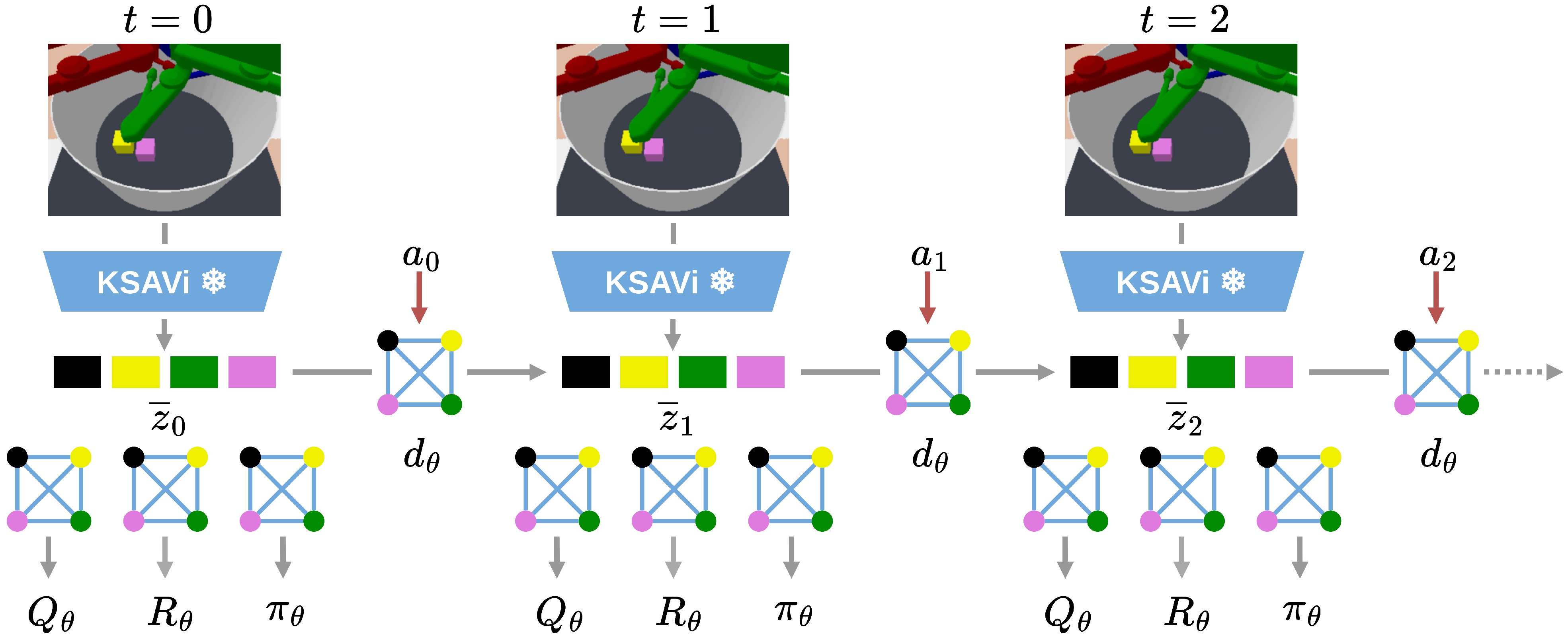
KORL extends TD-MPC2 (Section 3.1)and uses KSAVi as an object-centric encoder. To process sets of object states, we employ graph neural networks (GNNs), which have proven effective for handling graph-structured data in reinforcement learning tasks [73] and for world modeling in environments with multiple objects [74].

World models based on GNNs enable implementing an inductive bias for object-centric and relation-centric representations of complex structured dynamical systems [75,76]. In particular, their ability to learn interactions between objects by explicitly taking into account the structured nature of such tasks enables outperforming monolithic approaches in terms of predictive accuracy in compositional environments involving multiple interacting objects [77]. Furthermore, GNNs have been shown to be effective as dynamics models in goal-conditioned robotic manipulation tasks [63]. Given the robustness of GNN-based world models, we hypothesize that a model-based object-centric agent built on a GNN-based world model can learn an effective policy.

Latent dynamics model $d_{\theta }$, reward model $R_{\theta }$, policy ${\pi }_{\theta }$, and action value model $Q_{\theta }$ are implemented as GNNs. The object states $\overline{z}$ are treated as node features of a complete graph and processed by these GNNs. The GNNs consist of node update functions node and edge update functions edge with shared parameters across all nodes. These functions are implemented as MLPs. The following expression provides an example of predicting the next object states ${\overline{z}}_{t+1}$ using the latent dynamics model $d_{\theta }$ given the current states ${\overline{z}}_t$ and action $a_t$ ($1\le i\le K$, K is the number of slots):

$${\mathtt{GNN}}_d:z_{t+1}^i={\mathtt{node}}_d(z_t^i,a_t,\sum _{j\ne i}{\mathtt{edge}}_d(z_t^i,z_t^j,a_t)).$$

(22)

The reward model $R_{\theta }$ and the state–action model $Q_{\theta }$ share a similar architecture with $d_{\theta }$ (Equation (22)), but they use a non-learned mean readout layer followed by an MLP to produce a single scalar value representing the entire graph. For example, the reward model is defined as follows:

$${\overline{u}}_R={\mathtt{GNN}}_R({\overline{z}}_t,a_t),{\widehat{r}}_t={\mathtt{MLP}}_R(\sum _{i=1}^K{u}_R^i/K).$$

(23)

The policy model ${\pi }_{\theta }$ does not take an action as input, and the output vector of the MLP is split into the parameters of a Gaussian distribution:

$${\overline{u}}_{\pi }={\mathtt{GNN}}_{\pi }\left({\overline{z}}_t\right),({\mu }_{\pi },log{\sigma }_{\pi })={\mathtt{MLP}}_{\pi }(\sum _{i=1}^K{u}_{\pi }^i/K).$$

(24)

Table 1. Comparison of the core model components and their primary implementations in KORL and TD-MPC2 for visual environments.

Component	TD-MPC2	KORL
Encoder, $h_{\theta }$	$z_t=\mathtt{CNN}\left(s_t\right)$	${\overline{z}}_t=\mathtt{KSAVi}\left(s_t\right)$
Latent dynamics model, $d_{\theta }$	$z_{t+1}=\mathtt{MLP}(z_t,a_t)$	${\overline{z}}_{t+1}=\mathtt{GNN}({\overline{z}}_t,a_t)$
Reward model, $R_{\theta }$	${\widehat{r}}_t=\mathtt{MLP}(z_t,a_t)$	${\widehat{r}}_t=\mathtt{GNN}({\overline{z}}_t,a_t)$
State–action value model, $Q_{\theta }$	${\widehat{q}}_t=\mathtt{MLP}(z_t,a_t)$	${\widehat{q}}_t=\mathtt{GNN}({\overline{z}}_t,a_t)$
Policy model, ${\pi }_{\theta }$	${\widehat{a}}_t=\mathtt{MLP}\left(z_t\right)$	${\widehat{a}}_t=\mathtt{GNN}\left({\overline{z}}_t\right)$

provides a comparison of the components in TD-MPC2 and KORL.

Effectively, we use the same objectives as in TD-MPC2: (Equations (4) and (8)). However, the encoder $h_{\theta }$ is not trained as we use frozen KSAVi models. Additionally, the latent state representation in KORL is a set of slots $\overline{z}$. Consequently, the first term in (Equation (4)) computes the mean squared error between sets of slots rather than between monolithic vectors representing the environment’s state, as in standard TD-MPC2. 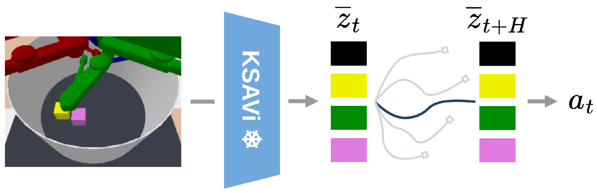Figure 2 illustrates KORL training, while Figure 3 shows the action-selection procedure in the environment.

3.6. Experimental Setup

We evaluate both the sample efficiency and the final performance of KORL against object-centric model-based and model-free RL algorithms across a diverse set of visually varied environments. We also compare the final performance of KORL with state-of-the-art monolithic MBRL algorithms.

3.6.1. Baselines

As object-centric baselines we consider three PPO-based [33] model-free methods: OCRL [10], OC-CA [14] and OC-SA [14]. These algorithms, as the proposed KORL, do not require any supervision to extract object-centric representations from the input image. The original version of the OCRL uses the SLATE [19] model as a slot extractor. In our experiments, we replace it with the KSAVi model as we were unable to train SLATE to achieve sufficient quality across all environments. Both KSAVi and SLATE use the Slot Attention module, which allows seamless integration of KSAVi into the OCRL architecture without changes to its transformer backbone, policy, or value heads. Refer to Appendix A.4 for the details for training the SLATE and the results of OCRL with SLATE model. OC-CA and OC-SA do not rely on a pretrained object encoder and learn their own object-centric representations as a set of vectors using cross-attention and self-attention mechanisms by attending to a patch grid. We use the SOLD [16] algorithm as an object-centric model-based baseline that employs SAVi [26] as the object-centric encoder. Additionally, we compare the final performance of KORL and SOLD against the state-of-the-art monolithic model-based algorithms TD-MPC2 [40] and DreamerV3 [3].

3.6.2. Environments

We evaluate our approach on object-oriented tasks across visually diverse robotic simulation environments, including CausalWorld [78], Isaac Gym [79], Robosuite [80], and ManiSkill [81]. In all environments, observations are 128 × 128 RGB images. Figure 4 shows examples of observations from the considered environments.

CausalWorld

In this environment, we experiment with the Object Reaching Task [10]. A fixed target object and a set of distractor objects are randomly placed in the scene. The agent controls a TriFinger robot and must reach the target blue cube with a green finger (the other two fingers are fixed) to solve the task. The reward function is sparse: the agent receives a positive reward only when it touches the target cube. The episode ends without reward if the green finger first touches a distractor object. The action space consists of three continuous joint positions for the movable finger, and episodes are limited to 100 steps. We report success rate as the performance metric.

Robosuite

In the Robosuite environment, we use the Block Lifting Task. A cube is placed on a tabletop in front of a single robot arm. The agent’s goal is to control the arm to lift the cube above a certain height. The position of the cube and the initial configuration of the robot are randomized. The reward function is dense. The action space consists of four continuous joint positions, and episodes are limited to 125 steps. We report return as the performance metric.

ManiSkill

In this environment, we use the Push Cube Task. The objective is to move a blue cube to a target position. Both the cube’s initial position and the goal position are randomized. The action space consists of three continuous joint positions. The reward function is dense. Episodes are limited to 100 steps. We report the success rate as the performance metric.

Isaac Gym

This task is inspired by an environment used in [57]. This task features a robotic arm in front of a table with a varying number of cubes in different colors. At the start of each episode, the cube positions are randomly initialized on the table. The agent’s goal is to push the cubes to predefined target locations. We experiment with three task variants: IsaacGym1C with a single red cube, IsaacGym2C with a red and a blue cube, and IsaacGym3C with red, blue, and green cubes. The target positions are fixed: the southeast corner of the table for the red cube, the southwest corner for the blue cube, and the northwest corner for the green cube. The action space consists of three continuous joint positions. The reward is proportional to the change in distance between the current and target coordinates of the cubes. Episodes are limited to 100 steps. We report return as the performance metric.

3.7. Object-Centric Encoder Pretraining

For each environment, we collect 300 K observations to train the object-centric encoders—KSAVi for KORL and OCRL and SAVi for SOLD. Separate KSAVi and SAVi models are trained for each environment. For Isaac Gym, the encoders are trained on data from the IsaacGym3C task and reused for all Isaac Gym tasks. After pretraining, KSAVi and SAVi are kept frozen.

3.8. Evaluation of Algorithmic Robustness of Object-Centric RL Methods

Robustness is a desirable property of control systems and algorithms, although its definition depends on the context. In robotics, robustness is defined as the ability of a system to resist disturbances that do not cause structural changes to the system [82]. Such disturbances include parameter uncertainty (e.g., payload, inertia, friction, and contact stiffness), sensor noise, and external perturbations. In the deep learning literature, the term is used in the context of adversarial robustness of neural networks to worst-case bounded perturbations [83,84], distribution-shift robustness [85], and perturbation robustness [86].

In deep RL, particularly in works focused on transferring policies from simulation to the real world, robustness is defined as the ability to maintain agent performance under worst-case transition and reward perturbations [87,88]. Another notion of robustness in deep RL arises from the high sensitivity of algorithm performance to hyperparameter choices [89], which necessitates task-specific tuning and incurs substantial computational cost. Recent state-of-the-art model-based RL algorithms, TD-MPC2 [40] and DreamerV3 [3], address this issue and exhibit algorithmic robustness: the ability to train an RL agent using a single fixed set of hyperparameters across a diverse task suite under a limited interaction budget while achieving consistent performance across all tasks. TD-MPC2 demonstrates consistent performance across 104 tasks using identical hyperparameters, and DreamerV3 exhibits robust learning across 150 tasks.

For object-centric RL, however, algorithmic robustness is additionally influenced by the quality of object-centric representations. The visual complexity of the environment directly affects representation quality, which in turn impacts policy, value, and world model learning. Consequently, the robustness of an object-centric RL agent depends on the robustness of its representation model, i.e., its ability to produce high-quality object-centric representations across visually diverse domains [90]. While RL agents may partially compensate for imperfect representations, this typically comes at the cost of reduced sample efficiency. We focus on the algorithmic robustness of object-centric RL agents as hyperparameter tuning for such agents is particularly expensive: object-centric representation models incur additional overhead compared to standard RL algorithms with holistic encoders.

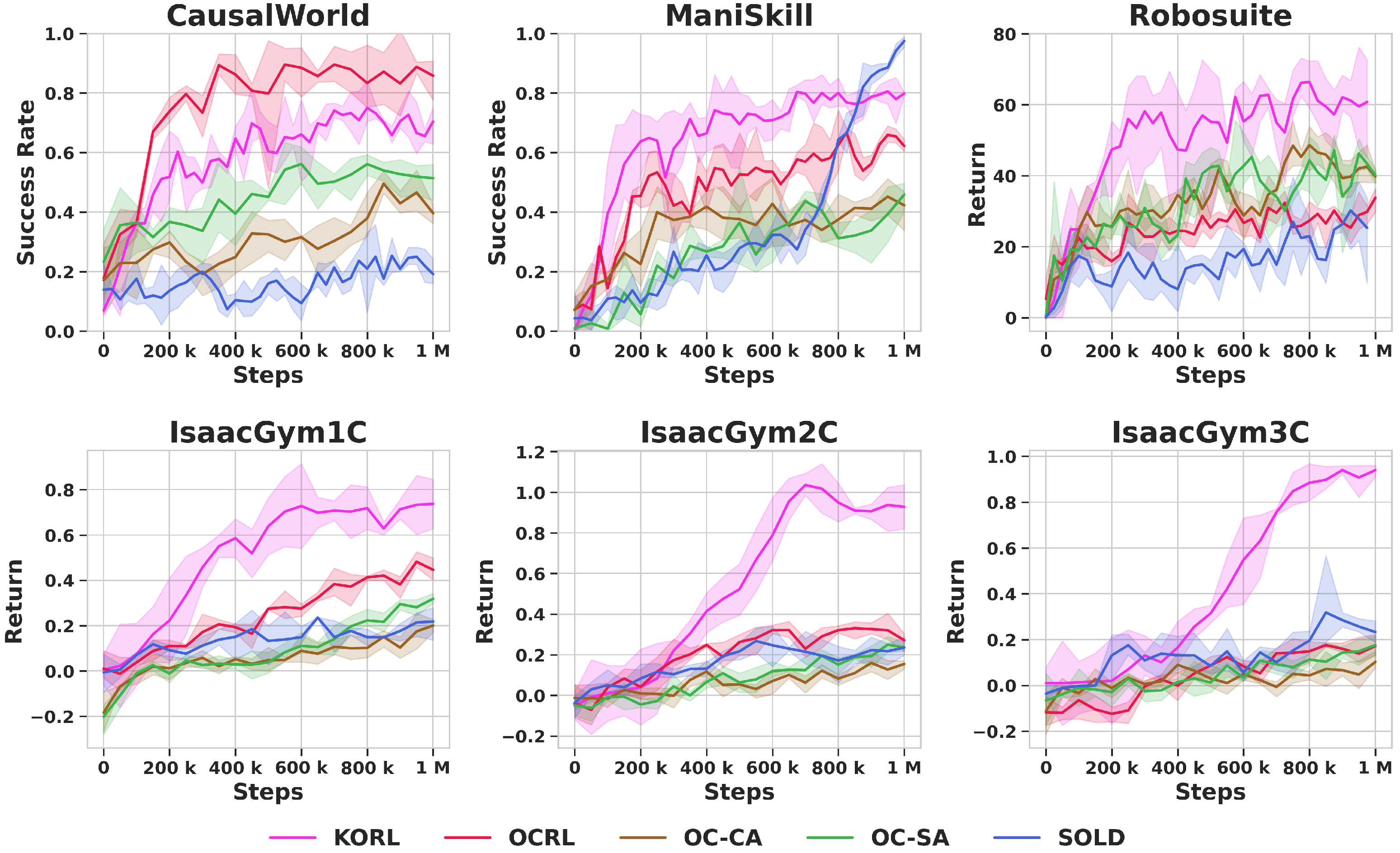
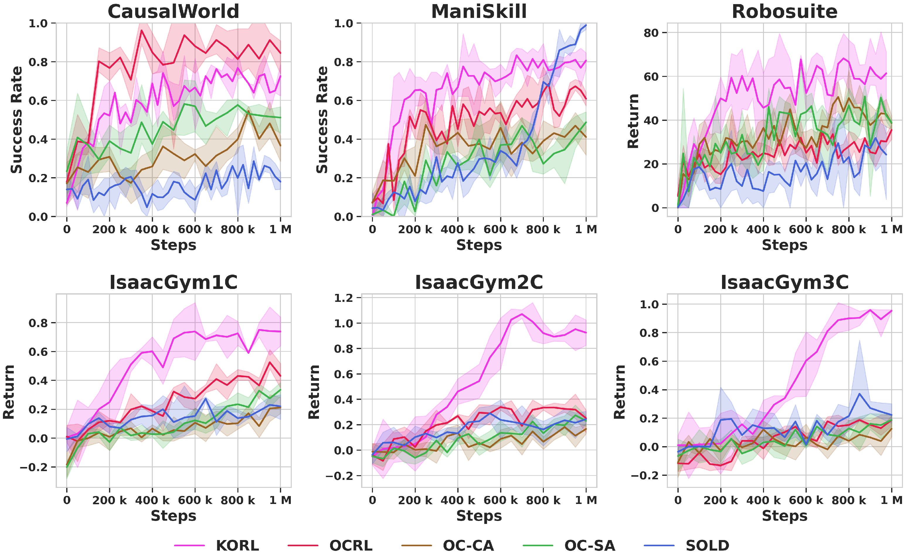
Our benchmark spans environments with varying visual complexity, ranging from relatively simple settings (e.g., CausalWorld) to more challenging ones (e.g., ManiSkill and Robosuite). To quantify algorithmic robustness under a fixed budget of 1 M environment steps, we compute the average performance across environments. To this end, we introduce a normalized score that aggregates an agent’s performance across a set of visually and dynamically diverse tasks into a single interpretable number. Because evaluation metrics (e.g., cumulative reward and success rate) differ in scale and nature across tasks, raw scores must be normalized prior to aggregation. We therefore normalize performance relative to the best-performing method in each environment.

Let $\mathcal{E}$ denote the set of environments. We define a normalized score $\mathcal{S}(m,e)$ for method m in environment $e\in \mathcal{E}$ and the mean normalized score $\widehat{\mathcal{S}}\left(m\right)$ that aggregates performance across environments. Let $M(m,e)$ denote the evaluation metric achieved by method m on environment e after 1 M training steps. The normalized score is defined as

$$\mathcal{S}(m,e)={\displaystyle \frac{M(m,e)}{{max}_{m^{\prime }}M(m^{\prime },e)}},$$

(25)

and the mean normalized score is given by

$$\widehat{\mathcal{S}}\left(m\right)={\displaystyle \frac{1}{\left|\mathcal{E}\right|}}\sum _{e\in \mathcal{E}}\mathcal{S}(m,e).$$

(26)

4. Results

For KSAVi, the best results are obtained with $K=6$ slots in the CausalWorld environment, $K=5$ slots in the Isaac Gym environment, and $K=3$ slots in the ManiSkill and Robosuite environments. Examples of attention maps are shown in Figure 4. In the CausalWorld and Isaac Gym environments, object and background separation is almost perfect. In the more visually challenging environments, ManiSkill and Robosuite, the background is partially mixed into the object masks.

The graphs in Figure 5 show how the success rate and episode return of the evaluated algorithms depend on the number of steps in the considered tasks (the curves without exponential smoothing are shown in Figure A3). In the Isaac Gym, Robosuite, and ManiSkill environments, KORL outperforms the object-centric baselines. CausalWorld is the only task on which the model-free OCRL algorithm performs better than KORL. Since OCRL and KORL share the same encoder (KSAVi), the comparison highlights that the model-free algorithm (OCRL) does not fully exploit the potential of object-centric representations in all tasks. In contrast, the GNN-based world model enables KORL to effectively plan trajectories in the slot-structured latent space, resulting in improved performance over the baselines. The inferior performance of SOLD can be attributed to the lower-quality scene decompositions produced by SAVi. For example, in the CausalWorld (Figure A11) and Isaac Gym tasks (Figure A13), SAVi encodes some cubes into the background slot, while, in the Robosuite task (Figure A12), the area around the edges of the red cube is also encoded into the background slot. In the ManiSkill environment (Figure A10), where SAVi clearly separates the robotic arm, the cube, and the target area from the background, SOLD and KORL achieve comparable performance. We also compare the intermediate and final performance of object-centric and monolithic model-based algorithms over a budget of 1 M environment steps, with the results reported in

Table 2. Performance comparison of model-based agents after 500 k and 1 M environment steps. The best result per environment is shown in bold, and the best object-centric result is underlined. Results are also highlighted where the standard deviations overlap with the best result. Averages and standard deviations are computed over three seeds and 30 episodes.

Step	Environment	Metric	Monolithic Agents		Object-Centric Agents
			DreamerV3	TD-MPC2	SOLD	KORL
500 k	CausalWorld	Success Rate	$\mathbf{0.80}\pm \mathbf{0.09}$	$\mathbf{0.66}\pm \mathbf{0.09}$	$0.18\pm 0.10$	$\mathbf{0.61}\pm \mathbf{0.11}$
	ManiSkill	Success Rate	$0.29\pm 0.07$	$\mathbf{0.82}\pm \mathbf{0.08}$	$0.28\pm 0.11$	$\mathbf{0.70}\pm \mathbf{0.08}$
	Robosuite	Return	$\mathbf{71}\pm \mathbf{12}$	$\mathbf{56}\pm \mathbf{9}$	$12\pm 8$	$\mathbf{57}\pm \mathbf{11}$
	IsaacGym1C	Return	$\mathbf{0.71}\pm \mathbf{0.09}$	$\mathbf{0.70}\pm \mathbf{0.10}$	$0.11\pm 0.06$	$\mathbf{0.70}\pm \mathbf{0.07}$
	IsaacGym2C	Return	$0.33\pm 0.09$	$\mathbf{0.89}\pm \mathbf{0.07}$	$0.24\pm 0.08$	$0.55\pm 0.10$
	IsaacGym3C	Return	$\mathbf{0.27}\pm \mathbf{0.10}$	$\mathbf{0.46}\pm \mathbf{0.13}$	$0.05\pm 0.09$	$\mathbf{0.38}\pm \mathbf{0.10}$
1 M	CausalWorld	Success Rate	$\mathbf{0.85}\pm \mathbf{0.10}$	$\mathbf{0.75}\pm \mathbf{0.08}$	$0.22\pm 0.12$	$\mathbf{0.71}\pm \mathbf{0.12}$
	ManiSkill	Success Rate	$0.38\pm 0.08$	$\mathbf{0.93}\pm \mathbf{0.06}$	$\mathbf{0.95}\pm \mathbf{0.06}$	$\underline{\mathbf{0.82}\pm \mathbf{0.09}}$
	Robosuite	Return	$\mathbf{89}\pm \mathbf{8}$	$\mathbf{79}\pm \mathbf{10}$	$23\pm 9$	$61\pm 12$
	IsaacGym1C	Return	$\mathbf{0.95}\pm \mathbf{0.07}$	$0.77\pm 0.09$	$0.21\pm 0.08$	$0.76\pm 0.10$
	IsaacGym2C	Return	$0.81\pm 0.06$	$\mathbf{1.09}\pm \mathbf{0.10}$	$0.24\pm 0.09$	$\mathbf{0.97}\pm \mathbf{0.09}$
	IsaacGym3C	Return	$\mathbf{0.99}\pm \mathbf{0.06}$	$\mathbf{1.05}\pm \mathbf{0.11}$	$0.24\pm 0.12$	$\mathbf{0.98}\pm \mathbf{0.10}$

. Overall, monolithic MBRL algorithms outperform object-centric methods. SOLD approaches the performance of TD-MPC2 after 1 M steps in the ManiSkill environment, where SAVi produces high-quality object-centric decompositions. KORL learns faster, outperforms SOLD, and achieves performance comparable to TD-MPC2.

Based on the performance after 1 M training steps, we estimate the robustness of object-centric algorithms using the mean normalized score (Equation (26)). Since we use three tasks from the Isaac Gym environment, we first average the normalized scores across the three Isaac Gym tasks before computing the mean normalized score.

Table 3. Mean normalized scores of evaluated object-centric agents across all environments. The best value is highlighted in bold. KORL achieves the highest score.

Object-Centric Agent	SOLD	KORL	OCRL	OC-CA	OC-SA
Mean Normalized Score	$0.44$	$\mathbf{0.82}$	$0.58$	$0.37$	$0.47$

shows that KORL is more robust than other object-centric algorithms across a visually diverse set of environments, achieving a higher mean normalized score. The normalized scores for all the algorithms and environments are listed in

Table A2. Normalized scores (Equation (25)) of the evaluated algorithms. Scores are computed as the ratio of each algorithm’s final performance metric value to the best value achieved for each environment. The best metric for environment is highlighted in bold.

Method	CausalWorld	ManiSkill	Robosuite	Isaac1C	Isaac2C	Isaac3C
DreamerV3	$\mathbf{1.00}$	$0.40$	$\mathbf{1.00}$	$\mathbf{1.00}$	$0.74$	$0.94$
TD-MPC2	$0.88$	$0.98$	$0.89$	$0.81$	$\mathbf{1.00}$	$\mathbf{1.00}$
SOLD	$0.26$	$\mathbf{1.00}$	$0.26$	$0.22$	$0.22$	$0.23$
KORL	$0.84$	$0.86$	$0.69$	$0.80$	$0.89$	$0.93$
OCRL	$0.99$	$0.65$	$0.38$	$0.46$	$0.21$	$0.18$
OC-CA	$0.45$	$0.43$	$0.42$	$0.23$	$0.16$	$0.10$
OC-SA	$0.59$	$0.58$	$0.43$	$0.39$	$0.20$	$0.20$

. The training details of KSAVi, KORL, and the baselines, as well as additional visualizations, are provided in Appendix A. For completeness, we train SDAC [45], a novel sample-efficient model-free off-policy algorithm based on SAC [35], on the considered tasks. Details of adapting SDAC to our tasks are provided in Appendix A.3. Learning curves of the monolithic algorithms TD-MPC2, DreamerV3, and SDAC are presented in Figure A5.

4.1. Evaluation of KORL’s Generalization Capabilities

Object-centric approaches are expected to generalize better than monolithic models [91]. To test KORL’s generalization, we evaluate its zero-shot performance on a modified version of the ManiSkill task with a significant change in scene appearance. We hypothesize that KORL’s slot-structured representations allow it to capture the compositional structure of the environment and distinguish task-relevant slots from non-informative ones. Consequently, scene changes that mainly affect non-informative slots should not degrade performance. In contrast, monolithic models such as TD-MPC2 and DreamerV3 operate on holistic representations, making it harder to isolate task-relevant features.

In the modified ManiSkill task, the floor texture is replaced with a uniform red color. Figure 6 shows that KSAVi still produces meaningful decompositions despite this change, with the new red area mainly assigned to the background slot.

Table 4. Success rates of KORL, TD-MPC2, and DreamerV3 under a visual distribution shift. Monolithic MBRL agents drop to zero when evaluated in the modified environment, while the success rate of KORL decreases by only 12%. Averages and standard errors are computed over three seeds and 50 episodes. The best metric is highlighted in bold.

Environment	DreamerV3	TD-MPC2	KORL
ManiSkill	$0.38\pm 0.08$	$\mathbf{0.93}\pm \mathbf{0.06}$	$0.81\pm 0.09$
ManiSkill (red floor)	$0.00\pm 0.00$	$0.00\pm 0.00$	$\mathbf{0.72}\pm$

reports the performance: the monolithic agents degrade to zero, whereas the performance of KORL decreases by only 12%.We attribute the performance degradation of KORL to background information being encoded in the slot corresponding to the robotic arm, meaning that changes in background color can influence the policy.

4.2. Comparison with SlotContrast

In the ManiSkill and Robosuite environments, some background regions are mixed into KSAVi slots corresponding to the robotic arm and the cube (Figure 4), which may degrade KORL’s performance. To investigate whether improved slot extraction can address this issue, we integrate SlotContrast [18], a state-of-the-art object-centric video model, into KORL. We refer to this variant as KORL:SlotContrast. It follows the KORL architecture but replaces KSAVi with SlotContrast for slot extraction.

Figure 7 shows attention maps produced by SlotContrast. Background information is still partially mixed into slots corresponding to the robotic arm and the object. Figure 8 presents the learning curves for KORL and KORL:SlotContrast, showing that KORL outperforms KORL:SlotContrast (the curves without exponential smoothing are shown in Figure A4). SlotContrast is trained to reconstruct features produced by a DINO encoder, whereas KSAVi is trained not only to reconstruct features from the AKOrN encoder but also to reconstruct the input image. We attribute KORL’s better performance to the richer information contained in KSAVi slots, which can be exploited by the world model and policy, resulting in higher sample efficiency. Further details on SlotContrast training are provided in Appendix E.

5. Limitations

Despite recent progress in unsupervised object-centric learning, current state-of-the-art models such as DINOSAUR [20], SlotContrast [18], and AKOrN [25] still struggle to decompose complex realistic scenes into distinct objects. We consider this limitation a major obstacle to applying object-centric RL algorithms—based on unsupervised object-centric encoders—in arbitrary environments. Moreover, since we represent the environment’s state as a complete graph of object states processed by GNNs, the computational complexity of KORL components becomes quadratic in the number of slots produced by the object-centric extractor. This design can lead to performance issues in environments containing a large number of objects.

6. Conclusions

In this work, we introduced KORL, an object-centric model-based RL method that leverages a pretrained object-centric encoder, KSAVi, combining Slot Attention with Kuramoto oscillatory neurons. Experiments on visually diverse robotic manipulation tasks show that KORL solves these tasks effectively and achieves more robust performance than existing object-centric model-free and model-based baselines. The results suggest that a GNN-based world model can effectively exploit object-centric representations. KORL also demonstrates zero-shot generalization under significant background appearance changes, while monolithic model-based methods fail. Finally, we show that KSAVi is more suitable for RL tasks than SlotContrast [18], a state-of-the-art object-centric video model, as replacing KSAVi with SlotContrast reduces performance.

One direction for future work is to explore transformer-based and other alternative architectures within the KORL framework. Another practically important direction is improving the resilience of the proposed KORL agent. In robotics, resilience is commonly defined as the ability of a system to recover its functionality after the robot is partially damaged [82,92,93]. Since our main contribution concerns the integration of a model-based RL algorithm with an object-centric representation model, we consider the scenario in which visual sensor input changes drastically due to damage. For example, if the appearance of the robot changes significantly after damage, both the object-centric representation model, KSAVi, and the world model should rapidly adapt to the new conditions and correctly identify which slot corresponds to the robot in order to restore performance. For KSAVi, this means handling a previously unseen object category. In turn, the world model and policy should be extended to cope with non-stationarity, including unanticipated changes in the environment. A possible approach to addressing this problem is continual and lifelong RL [94,95].