Article

EEG-Based Emotion Dynamics Recognition Using Hybrid AI Models for Cybersecurity

by
Ekaterina Pleshakova
1,*,
Aleksey Osipov
1,
Alexander Yudin
1 and
Sergey Gataullin
1,2
1
MIREA—Russian Technological University, 78 Vernadsky Avenue, 119454 Moscow, Russia
2
Social Modeling Lab, Central Economics and Mathematics Institute, Russian Academy of Sciences, Nakhimovsky Pr., 47, 117418 Moscow, Russia
*
Author to whom correspondence should be addressed.
Technologies 2026, 14(4), 209; https://doi.org/10.3390/technologies14040209
Submission received: 22 January 2026 / Revised: 12 March 2026 / Accepted: 25 March 2026 / Published: 31 March 2026

Abstract

The effectiveness of social engineering schemes, such as phishing, depends significantly on the victim’s emotional state, which is intentionally moved by the attacker toward fear, sadness, and disgust through time pressure, threats, or messages about potential losses, which weaken cognitive control. EEG datasets that simultaneously contain basic emotions and realistic phishing scenarios are lacking. Therefore, in some cases, stress-based biophysiological datasets obtained using the Trier Social Stress Test (TSST) are used for neurophishing modeling. The TSST exhibits phasic dynamics: a transition from a neutral state to a peak in fear, followed by an increase in sadness and a partial recovery to a neutral state, highlighting fear and sadness as key components of social stress. The interval of maximum fear probability is interpreted as the window of greatest vulnerability to phishing, when it is critical to consciously pause, verify information across independent channels, and avoid impulsive actions. The suggested hybrid neural network model, WS-KAN-EEGNet, is trained on five emotions and applied to these recordings, generating temporal trajectories of state probabilities with high accuracy, forming a reliable basis for future industrial solutions to ensure a secure digital space.

1. Introduction

As threats and vulnerabilities in the digital space grow, so does the need to develop effective detection and countermeasure tools capable for creating a secure and comfortable digital environment. The development of generative artificial intelligence and high-performance computing is shifting the cybersecurity paradigm [1,2] towards automated, intelligent systems based on deep learning, which are proving highly effective in detecting incidents and countering social engineering attacks. Intelligent systems can analyze text and multimodal information, identifying anomalous behavior patterns and predicting potential threats [3,4]. At the same time, to ensure high accuracy, interpretability, and computational efficiency in such systems, it is advisable to develop novel algorithms adaptable to complex, evolving attacks [5,6]. The use of Kolmogorov–Arnold networks (KANa), based on Kolmogorov’s theorem on the superposition of multidimensional functions, serves as a large-scale direction in the field of compact, interpretable and high-performance models [7]. It is worth noting that their practical application in ensuring the security of the digital space remains insufficient due to high computational complexity and the lack of adaptive learning algorithms. This paper presents a hybrid neural network model combining KAN with classical machine learning methods, including convolutional neural networks and wavelet transforms. The authors continued research into a possible increase in the hybrid neural network model’s efficiency for processing biosignals using the windowed Fourier transform, wavelet analysis, capsule, convolutional, recurrent neural networks, and numerical and other mathematical optimization methods for neural network structures, based on results obtained previously [8,9,10,11].
Emotions and cognitive states play a key role in user vulnerability to social engineering attacks, and their assessment using visual and neurophysiological signals opens up opportunities for the creation of interpersonal defense systems against phishing and smishing [12,13,14]. Below is a review that sequentially links computer vision, EEG analysis of emotions, and the concept of neurophishing.
Despite the extensive body of work on EEG-based emotion recognition, three critical gaps persist that this study addresses.
Gap 1: Architectural. No existing study has proposed a hybrid architecture that integrates KAN-based learnable one-dimensional activation functions directly into both temporal (1D) and spectral (2D) EEG processing branches within a unified ensemble framework. Current CNN models (e.g., EEGNet [15], DeepConvNet [16]) treat convolutional kernels as fixed scalar weights; Transformer-based approaches (e.g., ERTNet [17]) achieve attention-based modeling but at the cost of very high parameter counts and limited interpretability; topology-aware methods (STGATE [18], multi-source domain adaptation [19,20]) improve cross-subject generalization but do not exploit the Kolmogorov–Arnold representation theorem.
Gap 2: Application. While the conceptual link between emotional vulnerability and phishing susceptibility has been discussed [21,22,23,24,25], no prior work has applied a trained EEG emotion classifier to TSST-derived stress recordings to extract quantitative temporal trajectories of fear, sadness, and neutral states, and interpreted them as phishing vulnerability profiles.
Gap 3: Interpretability. Existing deep learning models for EEG emotion recognition provide limited insight into which spectral or temporal components drive classification decisions. The KAN framework, through visualization of learned univariate basis functions, offers a path toward neurophysiologically meaningful interpretability.
This study addresses these gaps by: (1) proposing WS-KAN-EEGNet, the first ensemble model combining wavelet-KAN convolutions (1D branch) and Stockwell-transform + KAN classification head (2D branch); (2) demonstrating through ablation that KAN-native blocks contribute a 3–5% accuracy gain over standard CNN/FC counterparts; and (3) applying the trained model to TSST EEG recordings to generate emotion probability trajectories, where the fear plateau is mapped to the phase of maximum phishing vulnerability.

1.1. Emotions in Computer Vision Systems

Modern facial expression recognition (FER) systems are widely used in education, medicine, operator monitoring, and security systems, relying primarily on deep learning methods and large datasets (FER2013, RAF DB, AffectNet) [12,13]. These studies are dominated by a taxonomy of basic emotions derived from Paul Ekman’s model, happiness, sadness, fear, anger, disgust, and surprise, to which neutral is almost always added as a separate class, forming a standard 6–7-class scheme for training and benchmarking.
The special role of five emotions—happiness, sadness, fear, disgust, and neutral—is emphasized in studies of recognition and error patterns: happiness and disgust are typically classified with high accuracy, while fear and sadness are often confused with each other or with neutral, reflecting the subtlety of visual cues and the peculiarities of human perception [26,27,28]. These features are taken into account when designing architectures and selecting metrics (confusion matrices, class-wise F1), as well as when implementing FER in critical scenarios where misinterpretation of fear or sadness may be more significant than an error in the happiness class [26,27,28].

1.2. Emotions and Cognitive States from EEG and Other Biosignals

In parallel with FER, the field of emotion and cognitive state recognition based on biorhythms, primarily EEG, but also heart rate variability (HRV) and electrodermal activity (EDA) [29,30,31], is rapidly developing. Recent studies employ both discrete emotion categories (often the same basic classes, including happy, sad, anxious/fearful, and neutral) and continuous valence–arousal models.
Choice of Discrete Emotion Framework. Although continuous valence–arousal models provide a richer affective space, the present work adopts discrete basic-emotion classification for three methodological reasons. First, the SEED-V dataset is natively labeled with five discrete categories (happiness, sadness, fear, disgust, neutral), making categorical classification the natural choice [32]. Second, the cybersecurity application requires detection of specific emotional states—primarily fear and disgust—that correspond to identified vulnerability mechanisms, rather than abstract dimensional shifts. Third, the temporal probability trajectories generated by the softmax output layer provide pseudo-continuous dynamics: the five-dimensional probability vector evolves smoothly over time, capturing fine-grained emotional transitions without requiring a separate valence–arousal regression model [33,34]. This discrete-to-continuous bridge avoids the lower test–retest reliability associated with subjective self-report scales used in continuous valence–arousal annotations.
However, in applied problems, classification of basic emotions and “stress/non-stress” remains the dominant approach.
Modern EEG models use CNNs, CNN-LSTM hybrids, and transformers trained on temporal, spectral, and temporal-frequency representations (STFT, CWT, filter banks) of multichannel signals [15,16,29,30,31,35,36].
Beyond conventional CNN/LSTM architectures, recent work has introduced topology-aware and transfer-learning frameworks for EEG-based emotion recognition. STGATE employs a spatial–temporal graph attention network with a transformer encoder to jointly model electrode-level time–frequency patterns and brain-region connectivity. Multi-source domain adaptation methods further improve cross-subject and cross-session robustness by inter-domain sample hybridization and dynamic contrastive domain adaptation across multiple source domains [18,19,20].
A typical pipeline includes:
  • Preprocessing (bandpass filtering, artifact removal, re-referencing);
  • Feature extraction in the θ (4–8 Hz), α (8–14 Hz), β (14–31 Hz), and γ bands;
  • Subsequent multi-class classification of emotional states and a neutral baseline.
The five core emotions—happiness, sadness, fear, disgust, and neutral—in this context retain the status of invariant “target classes” used in both visual and EEG approaches [29,30,31]. Happiness and sadness exhibit reproducible patterns of frontal asymmetry and power changes in the α/β bands, while fear and disgust are associated with patterns associated with stress and responses to threatening or unpleasant stimuli; the neutral state serves as a baseline for normalizing EEG activity [29,30,31].

1.3. Multimodal Architectures: FER and EEG Integration

Recent research has demonstrated a convergence between FER and EEG analytics architectures: both widely utilize CNN/ResNet-like networks, attention mechanisms, and transformers [37,38,39]. The target problem in both cases is formulated identically—multiclass emotion classification (including neutral states); only the input data types and encoding methods (facial images vs. topographic maps/EEG time spectra) differ.
Multimodal systems that combine facial video, voice, and EEG use a unified emotional taxonomy, where happiness, sadness, fear, disgust, and neutral serve as a “common language” across channels [37,40]. Such approaches demonstrate reduced confusion between closely related states (e.g., sadness vs. neutral) and increased resilience to noise in individual modalities, which is critical for real-world use in HCI and user experience monitoring systems.

1.4. Neurophysiological Susceptibility to Phishing and Neurophishing

Phishing attacks via SMS (smishing) and mobile messaging apps pose a growing threat to mobile subscribers. Unlike traditional technological defenses (filtering, blacklists), understanding the neurophysiological mechanisms of user susceptibility to phishing can significantly improve the development of interpersonal defense systems. Research shows that high cognitive load, stress, low vigilance, and knowledge deficits increase vulnerability to social engineering attacks, while physiological indicators of stress (EEG, heart rate variability, electrodermal activity) can reflect a user’s actual cognitive state more accurately than self-reports [21,22,23].
High cognitive load reduces the ability to detect deceptive cues in messages: when pre-loaded with cognitive load, phishing detection accuracy decreases from 84% to 76% [41], demonstrating the impact of cognitive overload on threat processing and critical thinking when reading messages. The cognitive psychology model of social engineering, described by Stajano & Wilson (2009) and reinterpreted in later work on cyber resilience, suggests that stress reduces the ability to detect deception in social engineering messages; this phenomenon is defined as “attentional tunneling,” in which focusing attention on the emotionally charged content of a message leads to ignoring peripheral warning cues [23].
The concept of neurophishing: Recent research describes “neurophishing” as adaptive attacks that monitor the user’s physiological metrics (including EEG) in real time and modify the message content to maximize success. This emphasizes the importance of understanding the neurophysiological mechanisms of susceptibility and shifts the emphasis from purely technological defenses to user-centric, neurophysiologically informed systems (e.g., adaptive interface warnings, blocking risky actions upon detection of an adverse cognitive state). Based on recent EEG research on cognitive stress and work on social engineering and physiological indicators of vulnerability, the following EEG markers are expected indicators of phishing attack perception:
  • Increased beta activity (14–31 Hz): associated with active cognitive strain and decision-making under pressure [21];
  • Decreased alpha activity (8–14 Hz): reflects a decrease in the relaxed state and activation of the frontal cortex [22];
  • Increased theta activity (4–8 Hz): associated with cognitive load, working memory, and suppression of involuntary attention [21,22];
  • Changes in the P300 component (event-related potential): a decrease in amplitude is recorded under high cognitive load and among individuals more susceptible to deception, making this indicator a candidate for online vulnerability assessment [42].

1.5. Integration of Emotions, EEG, and Anti-Phishing Protection

The link between emotional states and vulnerability to phishing is demonstrated by the fact that stress, fear, frustration (similar to sadness), and decreased vigilance increase the likelihood of making an erroneous decision under information pressure. The EEG markers described above can be viewed as a neurophysiological reflection of the transition from a neutral state to states of increased cognitive load and emotional tension, which have previously been analyzed in the context of EEG emotion recognition and multimodal systems [29,30,31].
Thus, a unified approach extends from basic emotions (happiness, sadness, fear, disgust, and neutral) in FER systems and EEG analytics to multimodal architectures and, ultimately, to the applied case of neurophishing. The use of real-time neurophysiological indicators creates the preconditions for adaptive protection systems that can, for example, enhance interface warnings or delay the execution of risky actions when the user’s EEG pattern indicates high cognitive load, stress, and, therefore, increased susceptibility to phishing attacks.
In parallel, transferable and topology-aware EEG emotion models have been proposed, including spatial–temporal graph attention networks with transformer encoders and multi-source domain adaptation frameworks that explicitly address inter-subject and inter-session distribution shifts via sample hybridization and dynamic contrastive alignment. These approaches demonstrate that cross-domain transfer and topology-aware representations can substantially enhance the generalization of EEG emotion classifiers, especially in subject-independent settings [18,19,20].
Overall, existing EEG-based emotion recognition and neurophishing studies, while increasingly sophisticated, still lack a unified and interpretable framework that jointly exploits both temporal and spectral EEG dynamics and explicitly links emotional trajectories to moments of highest susceptibility to phishing. Most current CNN- and Transformer-based models treat convolutional kernels and fully connected weights as fixed scalars, provide limited insight into which spectral–temporal components drive decisions, and do not directly operationalize concepts such as fear plateaus or neutral-state suppression as quantitative vulnerability markers. This methodological gap motivates the architectural and application-level choices made in the present work and sets the stage for the hybrid KAN-based approach developed in the following sections.
This study addresses these gaps by: (1) proposing WS-KAN-EEGNet, the first ensemble model combining wavelet-KAN convolutions (1D branch) and Stockwell-transform + KAN classification head (2D branch); (2) demonstrating through ablation that KAN-native blocks contribute a 3–5% accuracy gain over standard CNN/FC counterparts; and (3) applying the trained model to TSST EEG recordings to generate emotion probability trajectories, where the fear plateau is mapped to the phase of maximum phishing vulnerability via a three-stage cognitive model (threat perception → attentional tunneling → impulsive action).

2. Theoretical Part

2.1. Description of the Subject Area

Electroencephalogram interpreters rely on a number of external EEG features that may indicate characteristics or changes in a person’s psychological state. For convenience, EEG frequency analysis is divided into four rhythms: α (8–13 Hz), β (13–30 Hz), θ (4–8 Hz), and δ (0–4 Hz). Table 1 shows the relationship between the psychological states we study and EEG changes.
Fear primarily activates the amygdala–ventromedial prefrontal cortex (PFC) pathway, with elevated coherence in the γ-band (>30 Hz). Disgust is predominantly associated with insular cortex and basal ganglia activation, reflected in increased θ-activity in anterior temporal regions [43,44].
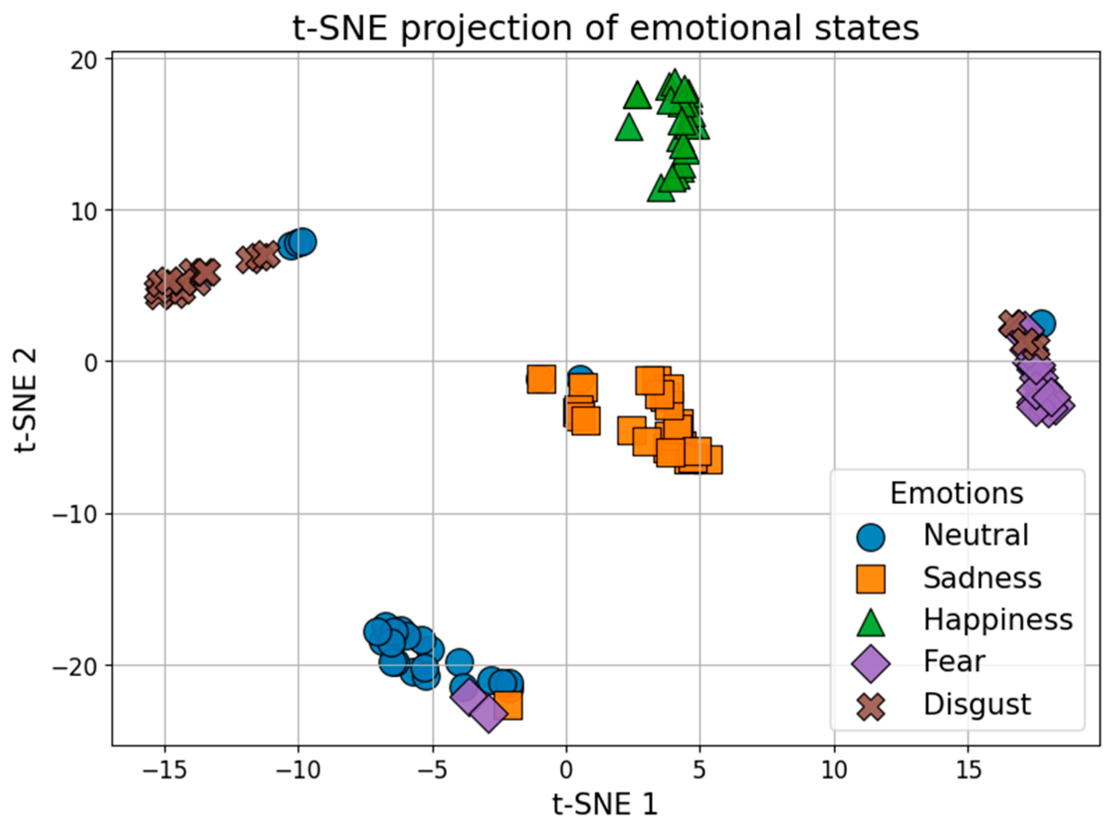
The model captures this distinction through the spatial attention mechanism in the second, 2D branch (2D-ST-KANCNN). In our experiments, the spatial attention weights for fear are concentrated in frontal-central regions (consistent with amygdala–PFC engagement), whereas for disgust the attention shifts toward anterior-temporal regions (consistent with insular cortex activation). This spatial differentiation enables the model to partially resolve the fear–disgust confusion observed in the t-SNE visualization (Figure 9), achieving per-class F1 scores of 0.89 for fear and 0.87 for disgust (see Section 2 and Section 4).
Table 2 summarizes the key characteristics of existing approaches—CNN, CNN-LSTM, Transformer, and KAN-based models—across four axes: interpretability, parameter count, feature representation type, and cross-subject generalizability. This table provides a structured comparison of EEG emotion recognition approaches along these axes and clarifies the methodological landscape for the proposed model. In particular, standard CNNs and CNN-LSTMs achieve good accuracy but remain difficult to interpret and often require large parameter budgets; Transformer-based models further increase parameter counts and depend on large datasets; and prior KAN-based work has not been systematically evaluated on EEG emotion benchmarks. By contrast, WS-KAN-EEGNet is explicitly designed to address these limitations by combining wavelet-based time–frequency representations with learnable KAN activations in both temporal and spectral branches, aiming to preserve interpretability while maintaining a compact parameter count and strong cross-subject generalization.
Limitations of Existing Approaches
Existing deep learning approaches for EEG emotion recognition exhibit several limitations: (i) standard CNNs are sensitive to the choice of frequency band and lack native time–frequency decomposition; (ii) LSTM-based hybrids have high parameter counts and are difficult to interpret; and (iii) Transformers require large datasets that are scarce in EEG research and offer minimal insight into which spectral components drive the decision. KAN-based architectures address these issues by replacing scalar weights with learnable one-dimensional functions (wavelets or splines), enabling: compact parametrization through the Kolmogorov–Arnold decomposition, interpretability via visualization of individual univariate basis functions, and native compatibility with wavelet representations of EEG signals.
Table 3 reveals several key patterns. First, classical pipelines on BCI Competition IV-2a, such as FBCSP (80.0% average accuracy) and EEGNet (73.55%), still require subject-dependent or within-subject evaluation protocols, whereas more recent methods on SEED and SEED-V ([17,45,46,47] and our WS-KAN-EEGNet) operate under subject-independent settings, which are generally more challenging. Against this background, the 91.3% subject-independent result of WS-KAN-EEGNet on SEED-V is particularly notable compared to prior SEED-V models, including CD-FTA (90.0%), CSET-CCA (82.06%), DAEST (73.6%), and ERTNet (67.17% ± 1.70%). Second, while FBCSP and DAEST rely on handcrafted or DE-based features, they are increasingly outperformed by end-to-end deep representations (EEGNet, DeepConvNet, CD-FTA, CSET-CCA, ERTNet, WS-KAN-EEGNet), highlighting the advantage of learned feature extractors. Third, no prior method on SEED-V has combined wavelet-based time–frequency decomposition with KAN-based learnable one-dimensional activation functions. The closest competitor on SEED-V, CD-FTA (90.0% under a subject-independent protocol), uses standard CNN attention without the approximation-theoretic advantages of the Kolmogorov–Arnold representation.

2.2. Wavelet Transform

The wavelet transform provides a time–frequency representation of a signal, allowing one to see when and at what frequencies signal components are present. A wavelet function (ψ) is a wave-like function with a rapidly decaying amplitude and a zero level. The wavelet function transforms the function under study into a two-dimensional surface:
x(t) ⟶ T(t, f),
where T(t,f)—contribution of frequency f at time t in the signal.
This paper uses two types of wavelet transforms: continuous (CWT) and discrete (DWT).
The wavelet transform for a continuous signal relative to a wavelet function is defined as follows:
T ( a ,   b )   =   1 a x t ψ * t b a d t ,
where ψ*—denotes the complex conjugate for ψ, the parameter b\inR corresponds to the time shift, and the parameter a > 0 specifies the scaling. In the discrete case, the scaling parameters a and shift b are represented by discrete quantities:
a = a 0 m , b = n b 0 ,
where m and n are integers.
Table 4 presents the main wavelet functions used in this work.
The Morlet wavelet balances temporal and frequency localization and is particularly effective for rhythmic EEG data. The Morlet wavelet, with its complex exponential modulation ( ψ ( t ) = c o s ( ω 0 t ) e t 2 / 2 ), provides a natural basis for capturing phase information—particularly the phase–amplitude coupling (PAC) phenomenon, where the phase of low-frequency oscillations modulates the amplitude of high-frequency activity [50,51].

2.3. Stockwell Transformation

The Stockwell transform (S-transform) is another approach to frequency–multiple-time analysis. This method is a “phase-corrected” version of the CWT. The S-transform can be thought of as a modification of the CWT that includes a specific parent wavelet multiplied by a phase-correction coefficient.
S ( t ,   f ) = f τ g t τ , f d τ ,
where g(t, f)—S-transform kernel constructed using a Gaussian window function:
g ( t ,   f )   =   1 2 π σ f e t 2 2 σ 2 f · e 2 π i f t ,
where σ(f)—a scale parameter that depends on the frequency f.
The Gaussian window function is used to analyze a signal in both the time and frequency domains.

2.4. Wavelet-Based KAN

KANs are a neural network architecture that is as versatile as a fully connected neural network, but more efficient and interpretable for specific tasks [52]. Unlike fully connected neural networks, decision surfaces, which are multidimensional functions, are approximated by one-dimensional functions, which significantly reduces the computational resources used by the neural network.
We use wavelets as approximating one-dimensional functions, which, according to A. M. Thant and T. Panitanarak, are the most promising option [52].
In the Wavelet-KAN method, the i-th neuron in layer l + 1 is determined by the formula:
x i l + 1 = j = 1 n ψ i , j x j l ,
where ψ i , j —parameter-tunable wavelet {wi,j, si,j, τi,j}. Wavelet selection is one of the goals of this article.
Neurons are combined into wavelet layers, and the layers form a complete network:
fWav−KAN(X(0))=T0(l+1, l)(…Ψ(1,0)(X(0))…)),
where X(0)—signal fed to the input layer of the neural network; Ψ(l+1, l)—wavelet transforms between layers of a neural network l и l + 1; and T0—an operator that transforms the results of successive wavelet transforms into a scalar (usually row summation).
It is necessary to clarify the applicability of the Kolmogorov–Arnold theorem to EEG data. The original theorem guarantees representation of continuous functions defined on compact sets [53,54]. In our framework, raw EEG signals are: (a) discretized at a fixed sampling rate (128–200 Hz), (b) segmented into fixed-length windows (quasi-stationary assumption), and (c) z-score normalized per channel, constraining the input to a bounded subset of ℝd. This satisfies the compactness requirement.
Discussion of KAT Applicability Under Non-Stationarity
The Kolmogorov–Arnold theorem requires the target function to be continuous on a compact domain. In EEG emotion recognition, the underlying neural process is inherently non-stationary—emotional states evolve over time, and the mapping from EEG patterns to emotional labels may exhibit abrupt transitions. We address this tension through the following reasoning:
First, the standard quasi-stationarity assumption in EEG processing segments the continuous recording into fixed-length windows (1–4 s for SEED-V), within which spectral properties are approximately constant. Each window is independently z-score normalized, constraining its input to a bounded, approximately compact subset of R d . The KAT is applied separately to each window’s local feature space, not to the entire recording duration.
Second, potential within-window transients (e.g., abrupt ERP components) are mitigated by the compact support of B-spline basis functions: a localized perturbation in the input affects only k + 1 adjacent basis functions, preventing error propagation across the entire spline representation.
Third, the temporal dynamics of emotion transitions are captured not by a single KAN evaluation but by the sequence of per-window softmax outputs, which forms smooth probability trajectories over time. This piecewise approach avoids requiring a single continuous function to span discontinuous emotional state boundaries [54].
We acknowledge that a fully rigorous treatment would require generalized KAN variants (e.g., piecewise-defined outer functions) or explicit segmentation of stationary regimes. The empirical success of our approach (91.3% accuracy under 5-fold cross-validation) suggests that the quasi-stationarity assumption is a reasonable practical approximation for emotion-length EEG windows. Taken together, these assumptions justify the use of the Kolmogorov–Arnold representation at the level of windowed EEG segments, while the concrete implementation in WS-KAN-EEGNet is realized through convolutional operators acting on local spatio-temporal patches. The high dimensionality (8 channels × L time steps) is handled architecturally: each Conv1DKolWavelet operates on a local window of one channel at a time, so that KAN one-dimensional functions φ i , j act on individual scalar elements of the convolutional window, and their summation forms the filter response—directly implementing the superposition scheme f x 1 , , x n = g i φ i , j x i

2.5. Wavelet-KAN Approximation

Neurophysiological Rationale for KAN in EEG Processing

The B-spline basis functions used in KANLayer possess compact support: each basis function B m ( z ) is non-zero only over k + 1 adjacent knot intervals. This mirrors the band-limited structure of EEG rhythms, where θ (4–8 Hz), α (8–14 Hz), β (14–31 Hz), and γ (>31 Hz) activity occupy well-defined, functionally distinct spectral windows (Table 1) [53]. By adjusting knot positions and spline coefficients during training, KAN layers can allocate discriminative capacity to amplitude ranges corresponding to specific EEG bands [55,56]—for example, dedicating more spline resolution to the β–γ boundary that differentiates fear-related frontal activation from disgust-related insular θ-activity.
In Conv1DKolWavelet, each scalar kernel weight in a standard Conv1D is replaced by a learnable univariate function φ k ( x ) = w x + m   c m B m ( ( x b ) / s ) . This transforms the convolution from a linear operation to an amplitude-dependent nonlinear filter. Consequently, the same temporal pattern (e.g., a 12 Hz α-spindle) can be modulated differently depending on its amplitude context, which is critical for discriminating emotional states that share spectral overlap but differ in power dynamics (e.g., fear vs. disgust both show β-increase but with different amplitude profiles).
For inter-channel phase synchronization—a key neural mechanism in emotion processing, particularly the amygdala–PFC γ-coherence pathway activated during fear—KAN’s per-edge univariate functions allow each pairwise channel interaction to be captured by its own nonlinear mapping, rather than a fixed scalar weight. This provides a richer representation of phase-coupling dynamics than standard convolutional kernels, which apply identical linear weights regardless of the amplitude or phase relationship of the inputs.
In our implementation, spline-based KANLayers are used in fully connected blocks, while wavelet-KAN convolutions play an analogous role in temporal convolutional layers; both rely on compactly supported univariate basis functions.
Recent work has extended KAN representations to state-space formulations for interpretable nonlinear system identification, demonstrating that KAN-based temporal models can achieve competitive performance with lower parameter counts compared to standard recurrent architectures [57].

3. Materials and Methods

3.1. Datasets and Experimental Protocol

To test the methods, the SEED-V dataset, collected by the BCMI laboratory [58], was used. This dataset was collected as follows:
  • Clips ranging from 2 to 4 min in length were selected, each evoking one of five emotions: happiness, sadness, fear, disgust, and neutral;
  • EEG recording devices were installed on 16 participants aged 19 to 24 years (including 10 women and 6 men), and they viewed three randomly selected clips (each clip was used three times);
  • The obtained results were saved as .cnt files, which were subsequently used for analysis.
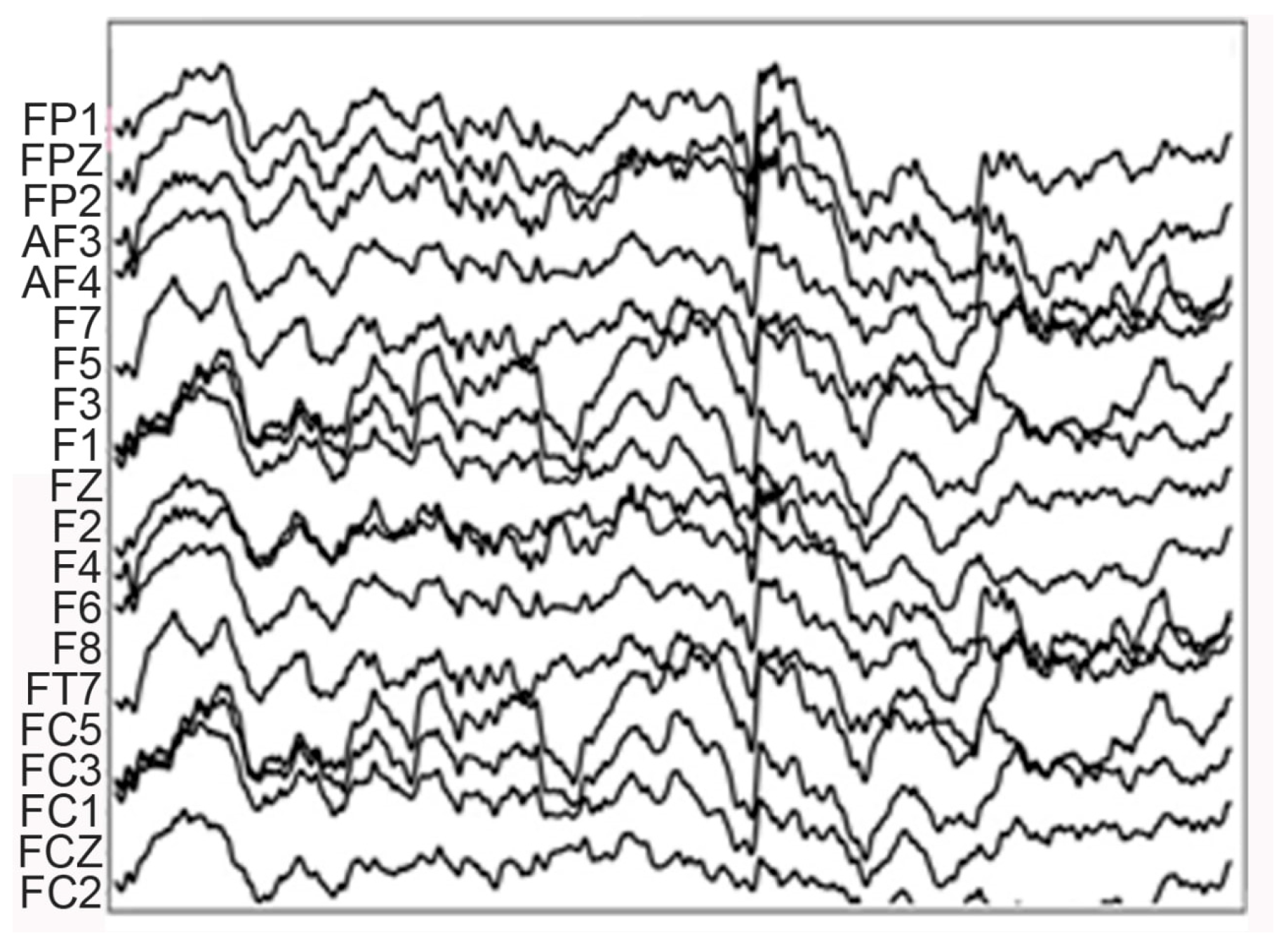
Overall, the dataset includes a total of 720 trials (i.e., 45 trials per participant for 16 participants). An example trial is shown in Figure 1.
Figure 1 shows an electroencephalogram obtained using the 62-channel ESI NeuroScan system. This figure represents 16 channels. The location of the sensors on the human head can be found in the work of W. Liu et al. [58].
To identify and quantify mental stress levels using EEG, we used the “An EEG Recordings Dataset for Mental Stress Detection” dataset hosted on the Mendeley Data platform [59].
The data were recorded using the EMOTIV EEG 5-Channel Sensor Kit/Emotiv Insight with electrodes AF3, AF4, F3, F4, Pz (or AF3, AF4, T7, T8, Pz in very similar sets), at a sampling rate of approximately 128 Hz, for several types of stress stimulation and 20+ subjects.
As shown by Khushboo Singh [60] and co-authors, emotional reactions are primarily manifested in changes in EEG signals recorded in the frontal and temporal regions of the brain. Additional channels have only a minor impact on accuracy, so we focused on these regions, as shown in Table 5.
Rationale for using two datasets.
The SEED-V dataset is used exclusively for training and evaluation of the five-class emotion classifier. The Mendeley stress dataset (TSST recordings) is used only at inference time: the pre-trained WS-KAN-EEGNet model is applied to the stress EEG recordings to generate temporal emotion probability trajectories, without any fine-tuning or re-training. There is no data leakage between the two datasets, as they serve fundamentally different roles (training vs. application).
Data partitioning and cross-validation.
For model evaluation on SEED-V, we employ 5-fold cross-validation with subject-independent splits: in each fold, data from 12–13 subjects form the training set, and data from the remaining 3–4 subjects form the test set. No data from the same subject appears in both sets, eliminating any within-subject information leakage.
Class balance.
SEED-V is balanced by design (144 trials per class across all subjects). Additionally, weighted cross-entropy loss is applied with inverse frequency weights to ensure robustness to minor class-level imbalances at the subject level.
Training protocol.
Optimizer: Adam (lr = 1 × 10⁻³, weight decay = 1 × 10⁻⁴). Batch size: 64. Maximum epochs: 100 with early stopping (patience = 15, monitoring validation loss). The 1D and 2D branches are trained independently, then frozen; the ensemble layer (2 parameters) is trained for 30 additional epochs.
Domain adaptation for stress dataset.
SEED-V uses a 62-channel system, while the Mendeley stress dataset uses 5 channels (AF3, AF4, F3, F4, Pz). For inference, we select the overlapping frontal channels (AF3, AF4, F3, F4, Pz) from both datasets, resample the stress data to match the SEED-V sampling rate, and apply the same z-score normalization pipeline.
Domain Adaptation for Cross-Dataset Inference
The systematic differences between SEED-V (62 channels, ESI NeuroScan, ~200 Hz) and the Mendeley TSST dataset (5 channels, EMOTIV Insight, 128 Hz) introduce a domain shift that affects inference reliability. We employ the following mitigation strategy: channel subsetting to the overlapping frontal montage (AF3, AF4, F3, F4, Pz), resampling and per-channel z-score normalization of TSST recordings to match the SEED-V preprocessing pipeline, and adaptive batch normalization (AdaBN), where batch-normalization statistics are recomputed on TSST data at inference time [48,49].
Table 6 reports the per-class mean softmax confidence on TSST recordings before and after AdaBN, along with the MMD values between SEED-V and TSST feature distributions. Table 6 summarizes the effect of adaptive batch normalization on cross-dataset inference quality: after AdaBN, the maximum mean discrepancy between SEED-V and TSST feature distributions decreases from 0.342 to 0.198, indicating a substantial (≈40%) reduction in domain shift, while the mean softmax confidence on TSST recordings increases across all emotion classes, with the largest gains observed for fear and disgust, suggesting that alignment of feature statistics leads to more stable and reliable emotion predictions under stress.
We acknowledge that more sophisticated domain adaptation techniques—adversarial domain obfuscation (DANN/CDAN) or multi-source contrastive adaptation—could further reduce the gap, and their integration with the WS-KAN-EEGNet architecture represents an important direction for future work.
Limitations of the TSST as a phishing proxy.
The Trier Social Stress Test elicits social-evaluative stress through HPA axis activation and sympathetic arousal, which overlaps with the neurophysiological response to phishing (β-band increase, α-suppression, and cognitive control degradation). However, TSST does not replicate phishing-specific cognitive biases such as loss aversion, authority compliance, or scarcity-driven urgency. We employ TSST recordings as a first-approximation proxy, and this limitation is further discussed in Section 5.1.
While TSST does not fully replicate a phishing attack—it does not engage loss aversion or authority compliance biases specific to fraud scenarios—it reproduces the core neurophysiological components of social stress (HPA axis activation, β-band increase, α-suppression) that underpin cognitive vulnerability, as summarized in Table 7. This positions our work as a foundational step toward real-time, neurophysiologically informed anti-phishing systems.
Preprocessing Pipeline Detail
The complete preprocessing pipeline consists of the following sequential steps:
  • Bandpass filtering: EEG signals are bandpass-filtered in the conventional 1–50 Hz range to remove DC drift and high-frequency noise (including power line interference), consistent with prior EEG emotion recognition studies.
  • Artifact handling: For SEED-V, standard artifact handling is applied, including removal of obviously corrupted segments and high-amplitude artifacts. For the Mendeley dataset (used only at inference), minimal preprocessing is applied due to the lower channel count and the auxiliary role of this dataset.
  • Segmentation: Continuous recordings are segmented into fixed-length windows in the range of 1–4 s, consistent with the quasi-stationarity assumption required for the Kolmogorov–Arnold framework and the window-based training of WS-KAN-EEGNet.
  • Channel selection: From SEED-V’s 62 channels, 8 frontal/temporal channels are selected (F3, F4, FC5, FC6, C3, C4, P7, P8) based on prior evidence of emotional signal localization [60,61,62,63].
  • z-score normalization: Per-channel z-score normalization is applied within each window to constrain inputs to a bounded subset of R d , which is consistent with the compactness assumptions used in the KAT-based analysis.
  • Time–frequency transform: A continuous wavelet transform (Morlet, cmor2.0-1.0) or S-transform is applied to each channel window to obtain time–frequency representations for subsequent processing.
  • Sobel filtering: Edge enhancement is applied to the resulting time–frequency maps (Sobel filtering) for the 2D branch to emphasize salient spectral–temporal structures.
Potential Biases and Limitations
Several potential biases in the datasets should be acknowledged: (a) the narrow age range (19–24) in SEED-V limits generalizability to other demographics; (b) all SEED-V recordings were obtained in controlled laboratory conditions, which may not reflect real-world EEG variability; (c) cultural homogeneity (Chinese university students) may introduce cultural bias in emotional expression; (d) equipment differences between SEED-V (research-grade ESI NeuroScan) and Mendeley (consumer-grade EMOTIV Insight) contribute to domain shift, partially mitigated by AdaBN (Table 6).

3.2. Data Processing Tools

The Python 3.9.13 programming language and the Tensorflow machine learning library were used to develop the algorithm. The experimental platform was equipped with a DEPO Storm 3450T4R server (DATSN.466219.013-03): SMD/2xG6230/1024GBRE16/L9361-8i/2DT480/4T4000G7/2DT960L/2DT960L/8HSDA/DATSN.469535.001/16D/6E/4GLAN/IPMI+/RTX3080/RTX3080/1200W2HS/FP/ONS3S. The system included 2 × G6230 processors (20 cores, 40 threads, 2.1 GHz, 27.5 MB cache, 125 W) and 1024 GB of RAM (8 × 128 GB DDR4 ECC REG).

3.3. Proposed Data Processing Algorithm

3.3.1. Model Testing Steps

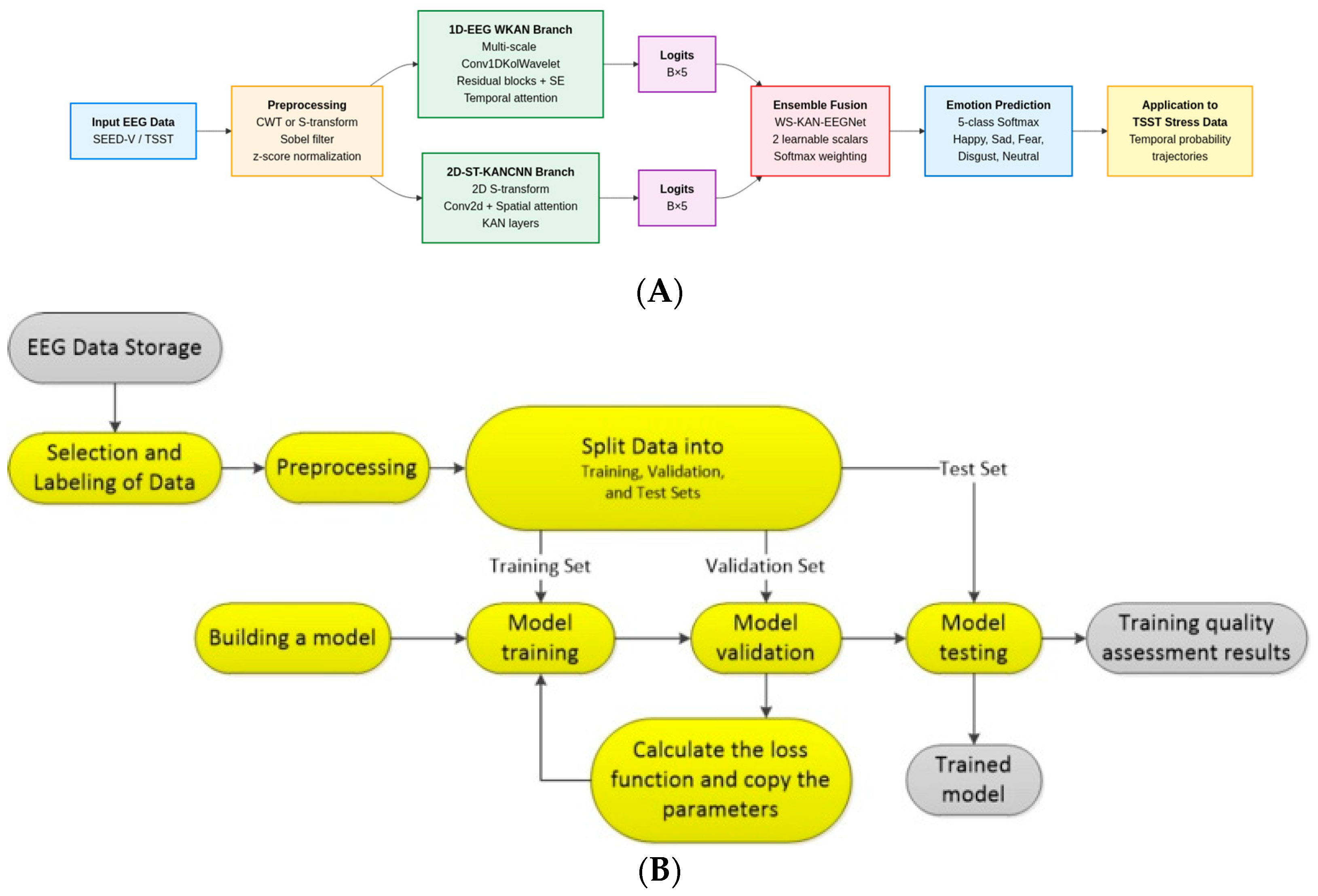
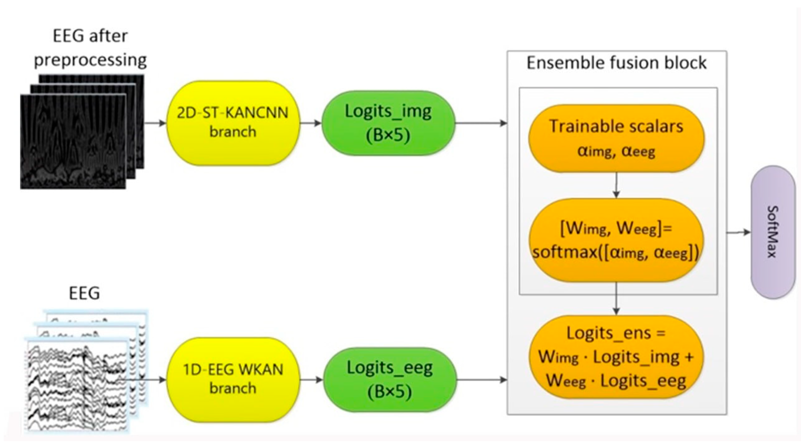
The overall WS-KAN-EEGNet processing and inference pipeline is summarized in Figure 2A.
Raw EEG data from the SEED-V dataset (used for training and cross-validated evaluation) or from the TSST stress dataset (used only at inference time) are first preprocessed using time–frequency transforms (continuous wavelet transform, CWT, or Stockwell transform, S-transform), Sobel edge filtering, and z-score normalization. The preprocessed signals are then fed in parallel into the 1D-EEG WKAN branch, which operates directly on multichannel temporal EEG signals, and the 2D-ST-KANCNN branch, which processes 2D time–frequency maps; each branch produces a vector of five-class logits (B × 5) corresponding to the target emotions (happiness, sadness, fear, disgust, neutral). These logits are combined by the WS-KAN-EEGNet ensemble fusion module with two learnable scalar weights that are normalized by softmax and used to compute a weighted sum of branch logits, and the fused logits are passed through a five-class softmax to obtain final emotion predictions, which are subsequently applied to TSST recordings to generate temporal trajectories of emotion probabilities.
The model testing algorithm can be divided into the following steps (Figure 2B):
  • EEG data are recorded and labeled by EEG specialists; in this work, we use pre-labeled recordings from the SEED-V and TSST-based Mendeley datasets [58].
  • The obtained data undergo a preprocessing step, which includes application of the continuous wavelet transform or Stockwell transform to the time series, followed by Sobel filtering of the resulting time–frequency representations and z-score normalization.
  • Training and test datasets are formed according to a subject-independent 5-fold cross-validation protocol on SEED-V, where in each fold the data from 12–13 subjects are used for training and the data from the remaining 3–4 subjects are used for testing, with no overlap of subjects between the sets.
  • The 1D-EEG WKAN and 2D-ST-KANCNN branches are trained on the SEED-V training folds using the protocol described in Section 3.3.3; after convergence, their parameters are frozen, and the ensemble fusion module with two learnable scalar weights is trained on SEED-V for an additional number of epochs.
  • The trained WS-KAN-EEGNet model is evaluated on the SEED-V test folds to obtain classification metrics and, without any fine-tuning, is then applied to the TSST stress recordings from the Mendeley dataset to produce temporal trajectories of emotion probabilities, which are further analyzed in the context of stress and phishing vulnerability.

3.3.2. Preprocessing

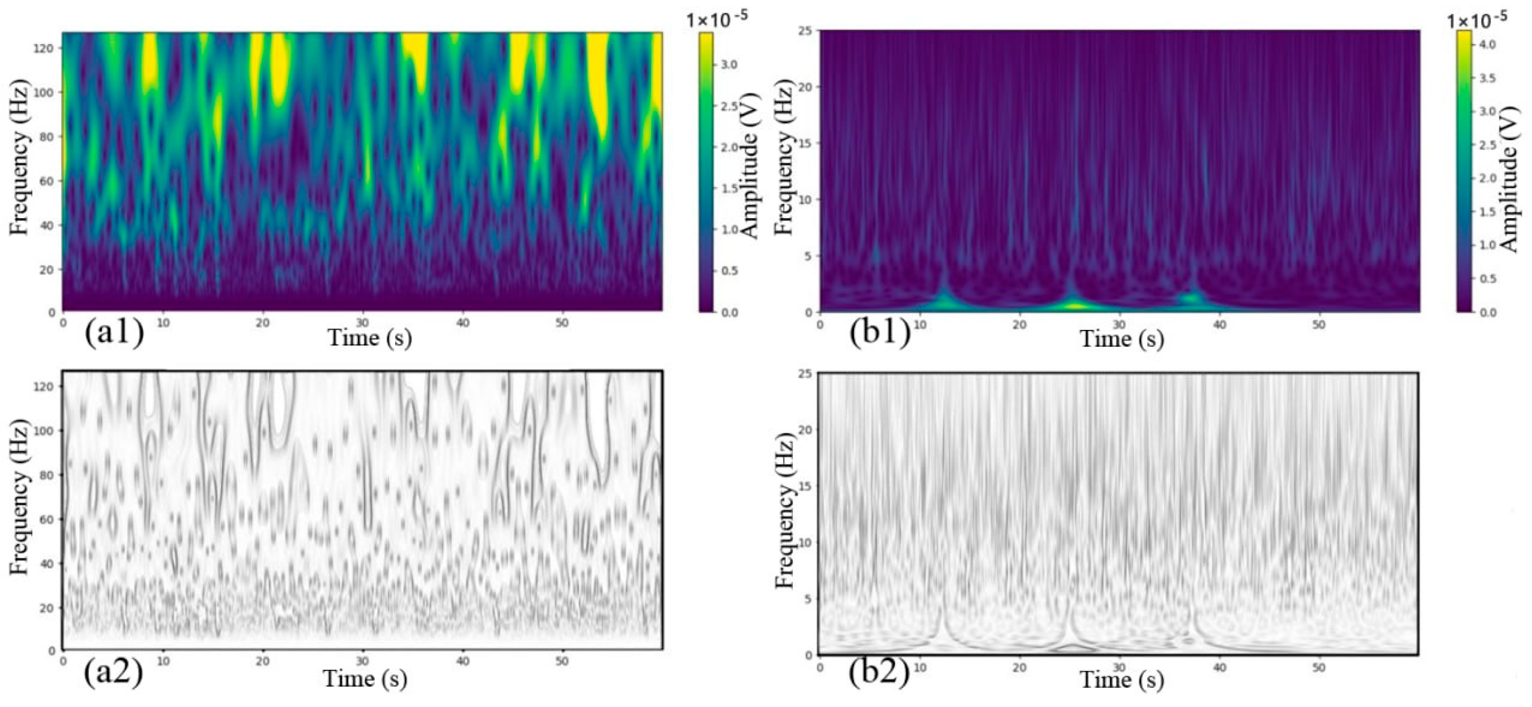
The preprocessing stage consists of the following substeps: first, the CWT or S-transform is applied, and then the resulting images are passed through a Sobel filter. One of our goals was to select the most suitable wavelet. The advantages of various wavelets are presented in Table 1. Figure 3 shows the complex Morlet wavelet cmor2.0-1.0. This wavelet corresponds to the general designation “cmorB-C” and is defined by the formula
ψ t = 1 π B e t 2 / B e j 2 π C t ,
where B is the bandwidth, and C is the center frequency.
The images in Figure 3 were obtained by processing the signal from the FPZ channel (frontal lobe) of a 23-year-old woman experiencing sadness.
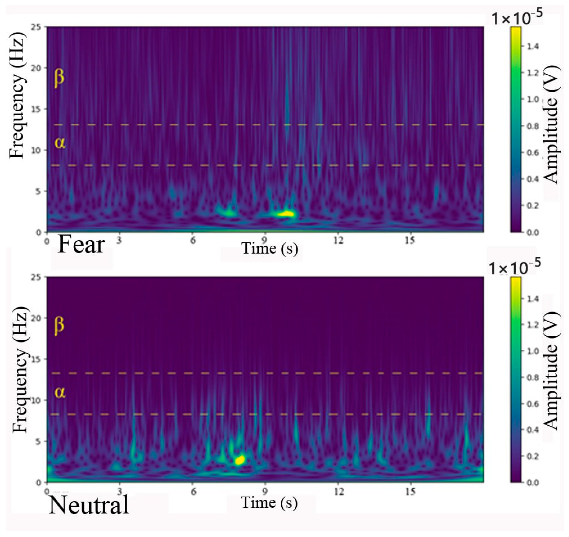
Figure 4 shows two time–frequency representations of the EEG, obtained using the S-transform, for the fear (upper graph) and neutral (lower graph) states.
In both spectrograms, the x-axis represents time in seconds, the y-axis represents frequency in hertz, with the α (approximately 8–13 Hz) and β (approximately 13–25 Hz) rhythm ranges highlighted, and the signal amplitude (in microvolts) is color-coded.
In the fear state, a more pronounced localized increase in power is visible in the low-frequency region (below 10 Hz) around the 8–9 s mark, while in the neutral state, a similar surge is less intense and more evenly distributed, illustrating the different activity patterns in these emotional states.

3.3.3. Model Construction

Based on the findings from the literature review and presented in the introduction, we selected a number of promising models. Each of these models is a neural network with convolutional layers for feature extraction and various classifier types. Depending on the neural network type, its input is processed using different methods. For simplicity, we divide these types into two categories: models that work with 1D function graphs and models that work with 2D images.
Building on this categorization, our proposed WS-KAN-EEGNet architecture combines both types within a unified ensemble. The WS-KAN-EEGNet architecture processes EEG data through two complementary branches. The 1D branch (1D-EEG WKAN) takes raw multichannel EEG time series and applies multiscale wavelet-KAN convolutions to capture temporal dynamics across multiple frequency resolutions, followed by temporal self-attention and global pooling. The 2D branch (2D-ST-KANCNN) takes the same EEG segments, converts them to time–frequency images via the Stockwell transform, and processes them through a CNN with spatial attention and KAN-based classification layers to capture spectral-spatial patterns. Both branches independently produce 5-class logits, which are fused by a lightweight softmax-weighted ensemble module into the final emotion prediction. The key innovation is that KAN one-dimensional learnable functions replace scalar weights at multiple levels (convolutional kernels in 1D, fully connected layers in 2D), improving approximation expressiveness while maintaining interpretability.
Model Working Directly with EEG Graphs
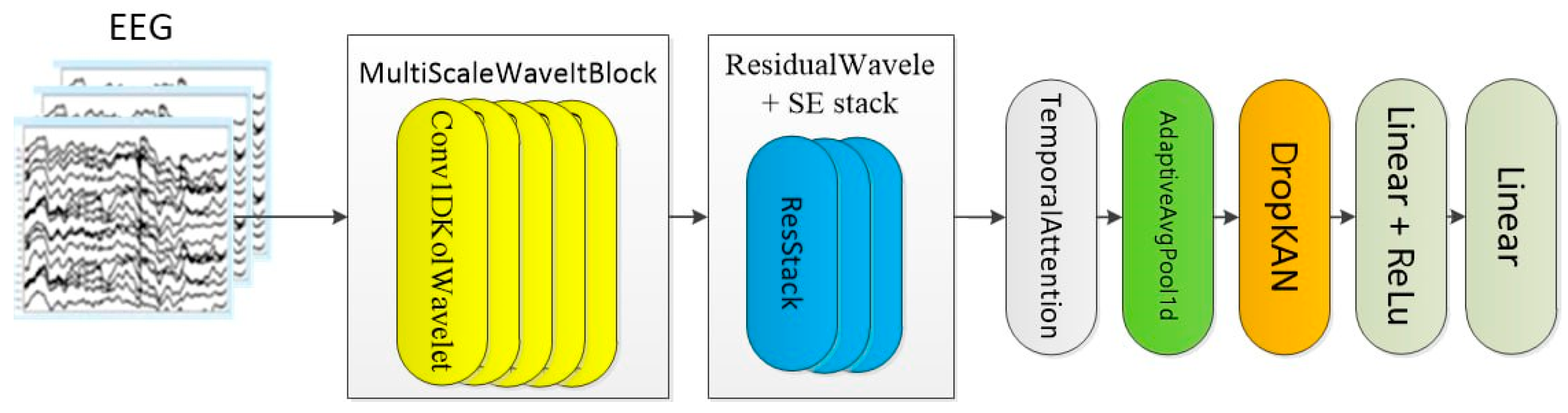
For working directly with EEG graphs, the 1D-EEG Wavelet–KAN branch (1D-EEG WKAN branch) neural network model is used. The model structure is shown in Figure 5.
The architecture of the 1D-EEG WKAN branch model is presented in Table 8.
The proposed model for analyzing multichannel EEG signals is a hierarchical architecture combining multiscale convolutions, temporal attention, and KAN-compatible blocks. The input is a B × 8 × L tensor; MultiScaleWaveletBlock computes five parallel Conv1DKolWavelet convolutions with kernels of 3, 5, 7, 9, and 15. Their concatenation with BatchNorm1d and ReLU forms a multiscale representation of 80 channels. KAN is integrated into the convolutional blocks so that instead of the usual scalar kernel weights, learnable one-dimensional functions (splines/wavelets) are applied to each element of the convolutional window, and their sums then form the filter response. In Conv1DKolWavelet and KANLinearWavelet, linear convolutional summation is complemented by such univariate functions on wavelet and spline bases, transforming each filter into a KAN-like operator and enabling the approximation of complex temporal dependencies through the superposition of multiple one-dimensional functions.
Then, three residual blocks with the Conv1DKolWavelet and SE modules sequentially expand the feature space to 128 channels, using shortcut connections to maintain a stable gradient. Next, the TemporalAttention module, based on multi-head self-attention (8 heads) with LayerNorm, models long-term temporal dependencies in a B × 128 × L tensor.
The AdaptiveAvgPool1d global time-averaging function compresses the sequence into a B × 128 vector, to which a DropKAN mask is applied as a stochastic regularization with zeroing and activity scaling. A classifier with two fully connected layers (128 → 64 with ReLU and 64 → 5) produces five-class logits.
This KAN-oriented and wavelet-boosted design approximates the complex EEG dependence across channels and time through the composition of one-dimensional operators and subsequent aggregation in residual and attention layers, enabling better capture of local and global patterns compared to classic CNN/RNN architectures.
Model for Preprocessed 2D EEG Images
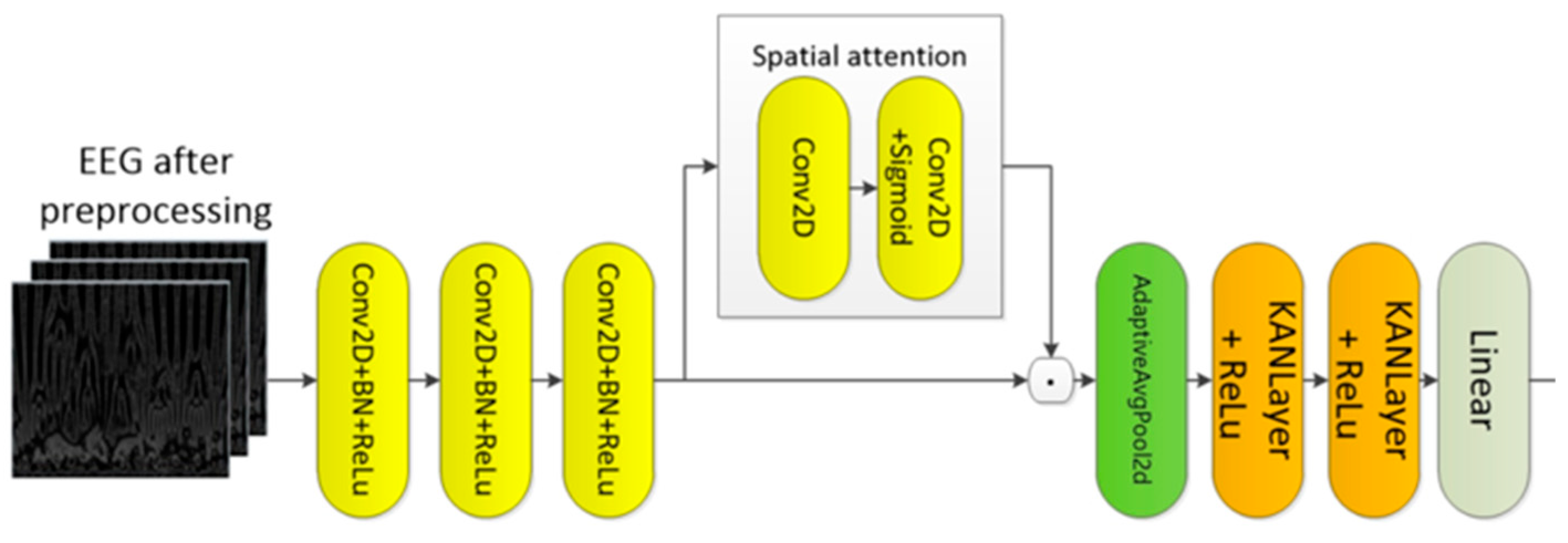
To process preprocessed data, the 2D Stockwell–KAN CNN branch (2D-ST-KANCNN branch) neural network model is used. The model structure is shown in Figure 6.
The architecture of the 2D-ST-KANCNN branch model is presented in Table 9.
The 2D-ST-KANCNN branch implements a hierarchical architecture for processing multi-channel EEG time–frequency representations, combining a 2D Stockwell-like transform, convolutional blocks, spatial attention, and a KAN-compatible classification head. The input is a tensor of 8-channel EEG time–frequency maps (B × 8 × 64 × 64). This tensor is processed by the STransform2D module, which performs a 2D Stockwell-like transform using a set of frequency-dependent Gaussian windows and an IFFT. This transform is followed by a cascade of three Conv2d–BatchNorm2d–ReLU blocks with a channel configuration of 8 → 16 → 32 → 48, which forms a hierarchical spatial-frequency representation, fed to the spatial attention module. The spatial attention module over the feature maps is defined by two sequentially applied convolutions: Conv2d(48 → 1, 3 × 3) with ReLU (aggregates information across channels into a single-channel importance map), followed by Conv2d(1 → 1, 3 × 3) with sigmoid (refines and normalizes the distribution to the range [0, 1]). Then, an element-wise x * attn multiplication is performed (a B × 48 × 64 × 64 feature map is multiplied by a B × 1 × 64 × 64 attention map). This enhances the informative regions of the time–frequency map before global aggregation.
The KAN-compatible classification head operates on the compact feature vector obtained after global averaging: AdaptiveAvgPool2d(1) collapses the spatial dimensions to (B,48,1,1). Next, squeeze removes redundant dimensions and forms a B × 48 tensor, which is fed into two layers, KANLayer(48 → 32) and KANLayer(32 → 16), with ReLU activation. Each KAN layer combines a linear projection and a B-spline component on the edges, improving expressiveness compared to a standard MLP. The final layer, Linear(16 → 5), maps the 16-dimensional representation to the logits of five classes, providing the spectral-spatial contribution of the 2D branch to the ensemble classification of EEG signals.
Ensemble Model, WS-KAN-EEGNet
To improve the performance of each individual neural network component, their ensemble model, the Wavelet–Stockwell Kolmogorov–Arnold Network for EEG classification (WS-KAN-EEGNet), is used. The model structure is shown in Figure 7.
The architecture of the WS-KAN-EEGNet model is presented in Table 10.
The fusion module implements a compact weight ensemble over two frozen branches: the 1D-EEG WKAN branch and the 2D-ST-KANCNN branch. The inputs are the B × 5 logits logits_img and logits_eeg; the base models themselves are not further trained at this stage, but are used only as prediction providers.
Within the module, two trainable scalars αimgeeg are defined, which are treated as modality importance logits and normalized by the softmax function into a weight vector [wimg,weeg] with a sum of 1. The final ensemble output is calculated as the weighted sum logits_ens = wimg⋅logits_img + weeg⋅logitseeg. Softmax is then applied to this weighted sum over 5 classes, and the predicted class is calculated.
Justification of fusion strategy.
With only two branches, complex fusion mechanisms (gating networks, cross-modal attention) introduce more parameters than semantically justified and risk overfitting on the relatively small SEED-V dataset (720 trials). The softmax-weighted fusion uses only 2 learnable parameters and consistently outperforms more complex alternatives, as shown in Table 11.
Per-class analysis.
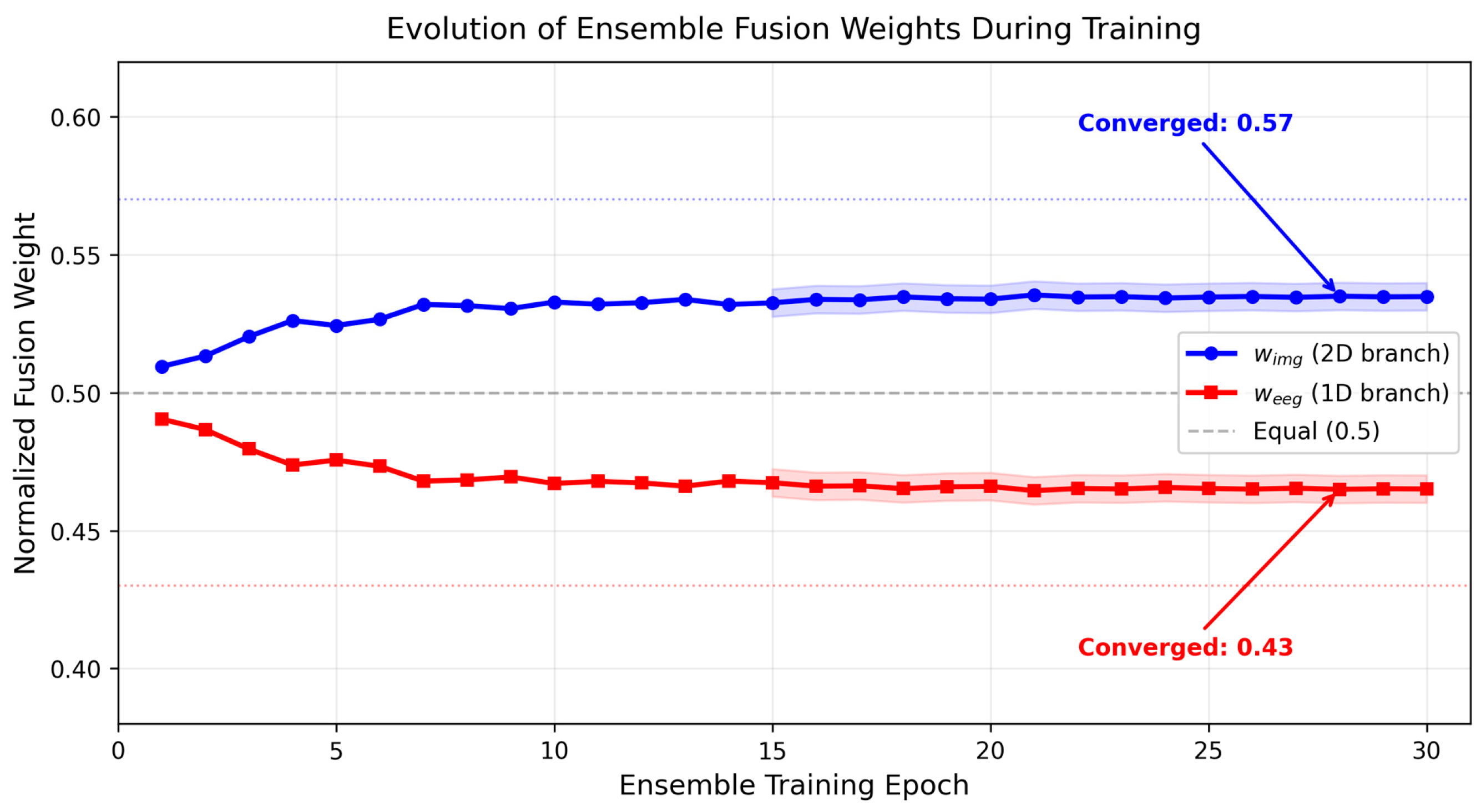
The learned weights converge to w_img = 0.57, w_eeg = 0.43, indicating that the 2D spectral branch contributes slightly more. Class-wise analysis reveals that the 2D branch excels at fear and disgust recognition (benefiting from spectral features), while the 1D branch is superior for happiness and neutral (benefiting from temporal dynamics).
Kolmogorov–Arnold Layers in the Model Architecture
The WS-KAN-EEGNet neural network incorporates a number of blocks using the KAN approach, directly based on the Kolmogorov–Arnold theorem. Pseudocode and a brief description of these blocks are provided below.
Block 1: KANLayer
Technologies 14 00209 i001
This block implements a Kolmogorov–Arnold layer that explicitly decomposes the mapping into basis functions (B splines), which conceptually follows the Kolmogorov–Arnold theorem on approximating multidimensional functions by the sum of one-dimensional ones.
Block 2: DropKAN mask
Technologies 14 00209 i002
DropKAN is a specialized variant of dropout for Kolmogorov–Arnold networks that operates on spline components in the KAN representation. It does not change the theoretical structure of KAN itself, but is a regularizer designed specifically for this architecture.
Block 3: KANLinearWavelet
Technologies 14 00209 i003
KANLinearWavelet combines wavelet preprocessing with a KAN representation: the output is given by the sum of a linear and spline path, which inherits the idea of a composition-sum representation of functions in the spirit of the Kolmogorov–Arnold theorem.
Block 4: Conv1DKolWavelet
Technologies 14 00209 i004
Conv1DKolWavelet implements a convolution where each local window is approximated by a KAN operator (KANLinearWavelet). Thus, the local mapping in each patch is structured as a KAN block, based on the idea of representing functions as sums of one-dimensional components.
Block 5: KANCNN (2D branch)
Technologies 14 00209 i005
KANCNN processes 2D S-transform maps through a stack of convolutional layers and spatial attention, then compresses the representation using global averaging and two sequential Kanban layers. This combines the power of CNN for local patterns and Kanban for flexible nonlinear feature classification.
Conv1DKolWavelet vs. standard Conv1D.
In a standard Conv1D, the kernel is a vector of scalar weights w k , and the output y ( t ) = k w k x ( t + k ) . In Conv1DKolWavelet, each scalar weight is replaced by a learnable univariate function, y ( t ) = k φ k ( x ( t + k ) ) , where φ k = w z + m c m ψ m ( ( z b ) / s ) . Here, w is the linear component, and the second term is a wavelet/spline expansion with learnable coefficients c m , shift b, and scale s. This transforms each convolutional filter into a KAN-like operator.
KANLayer vs. standard FC. A standard FC layer computes y = Wx + b (affine transformation). KANLayer computes y j = i [ w i j x i + s p l i n e i j ( x i ) ] , where s p l i n e i j is a B-spline with learnable control points. The key difference: each edge in the network possesses its own nonlinear activation function (the spline), rather than a shared activation applied after a linear transform. The spline parameters (grid points, coefficients, spline order) are the specific parameters distinguishing KANLayer from FC, and their concrete settings in WS-KAN-EEGNet are summarized in Table 12.

4. Experiments and Results

4.1. Overall Performance on SEED-V

Several neural networks were trained on the SEED-V dataset to detect emotions using EEG. The results are presented in Table 13.
The first two neural networks are the separately operating 1D and 2D branches of the WS-KAN-EEGNet ensemble model. Models 4–7 are presented for comparison. Other types of neural networks, which are unsuitable for the task of using a neural network with a different dataset in low-latency mode, are excluded from the comparison list. The presented data demonstrates that the ensemble model performs better than each of its components individually and than all baseline models. Its accuracy of 91.3% allows it to predict a person’s emotional state with high confidence, as summarized in Table 14.
The ablation study confirms: (a) the ensemble outperforms individual branches; (b) KAN-native blocks contribute +3.3% (1D) and +2.7% (2D) compared to standard Conv1D/FC replacements; and (c) learned fusion weights improve the result by +1.2% compared to equal weighting.

4.2. Temporal Emotion Dynamics and Cross-Dataset Application

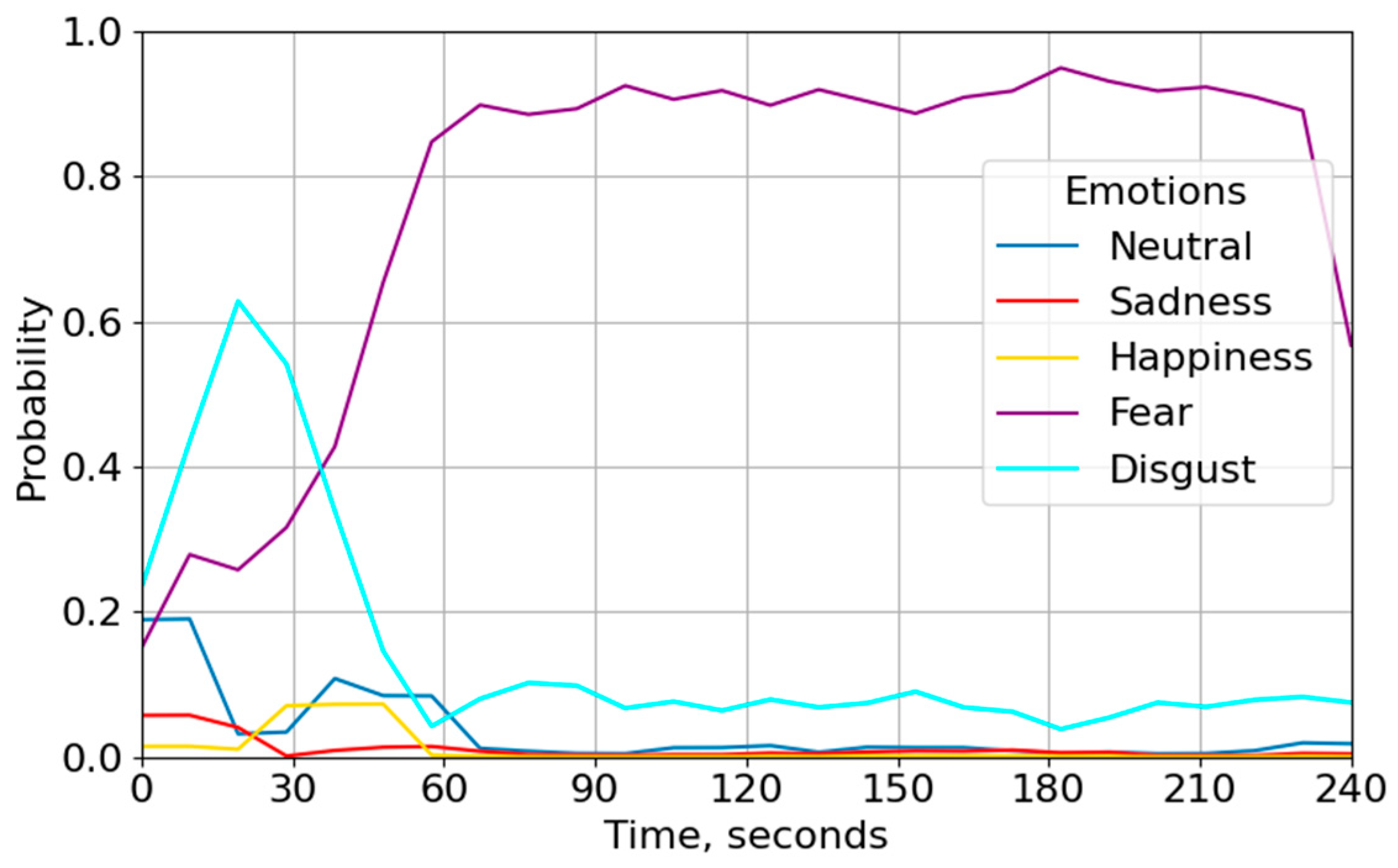
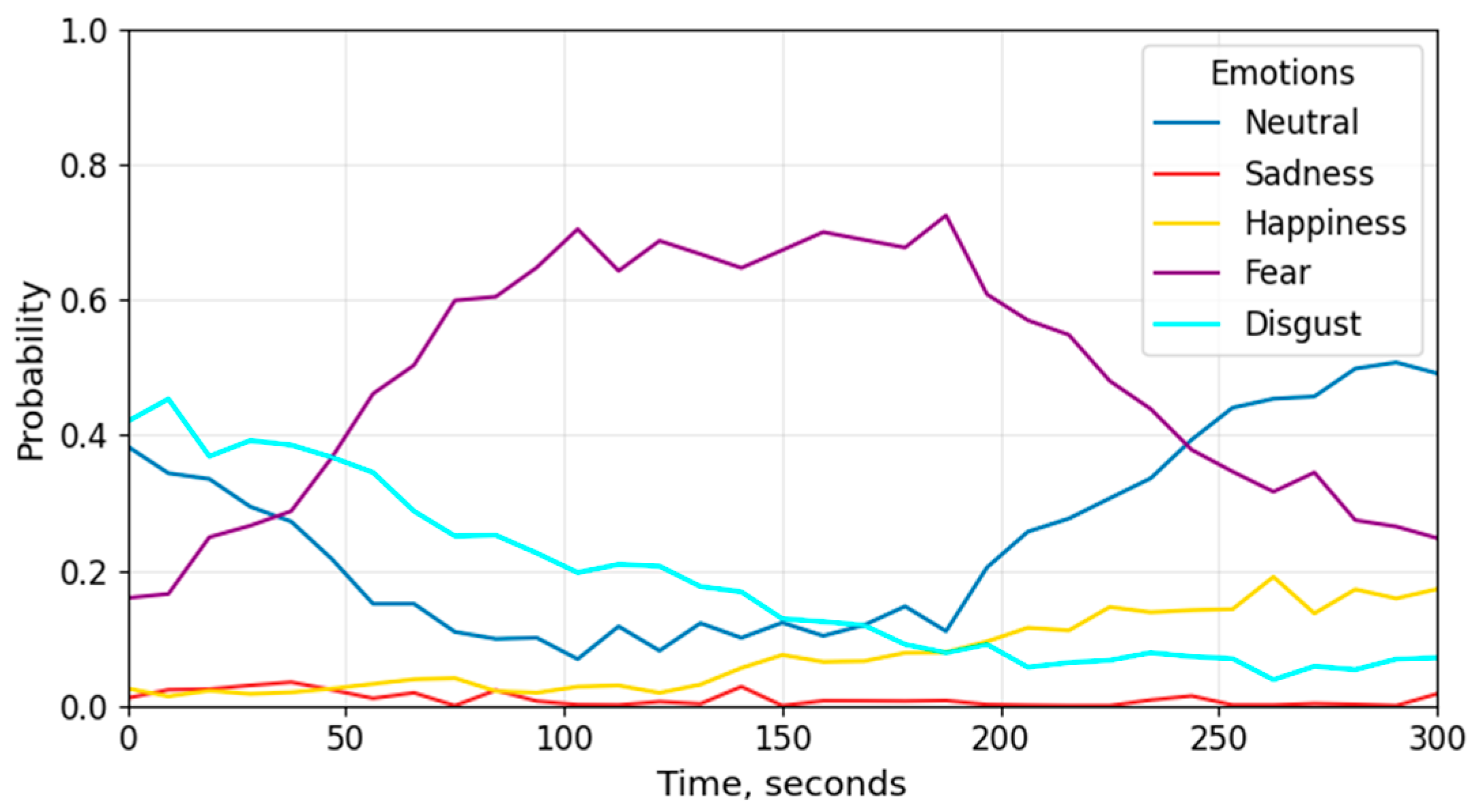
However, to decompose the concept of stress into its component basic emotions, we used the probabilities of the final layer of the SoftMax neural network to estimate the contribution of each emotion to a person’s overall state. Figure 8 shows the probabilities output by the WS-KAN-EEGNet neural network for each of its five output channels. The graph shows that disgust is partially involved in the emotion of fear, while other emotions are practically not involved.
To intuitively understand the differences between different human emotional states, we used the t-SNE algorithm. The data are taken from the final SoftMax layer of the WS-KAN-EEGNet neural network. As shown in Figure 9, the neural network distinguishes between various human emotional states quite well. However, only the happiness class is completely separable from the other classes. Quantitatively, the t-SNE embedding yields an overall silhouette score of S = 0.41, with the highest separability for happiness and reduced separability for fear vs. disgust, consistent with the confusion matrix. We are particularly interested in the states of fear and disgust, which we were unable to completely separate from each other.
We used the trained model to determine the range of emotions associated with social stress. We used the An EEG Recordings Dataset for Mental Stress Detection dataset. Figure 10 shows the probability trajectories from the final SoftMax layer of the WS-KAN-EEGNet neural network for a subject taking the Trier Social Stress Test (TSST) from this dataset.
The results demonstrate a typical response profile to socially evaluative threat and a sense of lack of control over the situation. Fear dominates the central portion of the plot, while the neutral state is suppressed and begins to increase only toward the end of stimulation, consistent with modern EEG studies presented in [64,65,66,67]. Conversely, the disgust curve shows an early and relatively short-lived rise followed by a decline, while happiness and sadness maintain low probabilities throughout the entire time interval (Figure 10). This is consistent with the results of studies on emotional stress and anxiety, where stressful states are distinguished from depressive and joyful ones [65,68]. The stable “plateau-like” maximum of fear in the middle of the recording is interpreted as reflecting maintained psychosocial stress, while the recovering increase in neutral and a partial increase in happiness at the end indicate a transition to a more adaptive state after the stressor is removed.
From a methodological perspective, the change in probabilities over time demonstrates that the EEG emotion recognition model is working correctly and is trustworthy. This is confirmed by the fact that, firstly, the model reproduces the expected course of the stress and fear response during long-term tasks: initially an increase, then a plateau, and then a decline, as described in modern EEG studies of stress and cognitive load. Secondly, the low level of sadness and only a moderate increase in happiness against a background of dominance of fear and disgust indicate that the classifier truly distinguishes between the anxious-stress circuit and other emotions, rather than reducing everything to a single “pleasant-unpleasant” axis. The resulting graph can be viewed as a visual temporal map of emotions, suitable for comparison with temporal-frequency EEG patterns, assessing the effectiveness of anti-stress interventions, and creating personalized mental state monitoring systems based on inexpensive EEG devices [64,65,66,67,69].
The emotional dynamics presented in Figure 9 are consistent with modern models of the perception of phishing and smishing attacks as forms of targeted emotional manipulation. Research shows that phishing messages systematically exploit fear, urgency, and the threat of loss to increase anxiety and impair decision-making, leading to an increase in errors and clicks on malicious links [24]. Experimental work with phishing email scenarios demonstrates significant links between physiological indicators of stress and vulnerability to attacks: participants exposed to emotionally charged messages are more likely to engage in risky behavior and are less likely to recognize fraud. Similarly, in the context of smishing messages and social media, the role of fear of missing out (FoMO) and anxiety about social/financial consequences has been noted, increasing users’ willingness to click links and disclose personal information.
Against this background, the temporal trajectory of emotion probabilities obtained from EEG (an increase in fear and disgust during the suppression of the neutral state in the central part of the protocol, followed by a restoration of neutral toward the end) can be interpreted as a universal pattern of emotional hijacking applicable to phishing and smishing scenarios. The peak of fear corresponds to the phase of maximum pressure (threat of account blocking, loss of money, or social reputation), when, according to behavioral studies, users are most prone to impulsive, ill-considered actions. Such patterns can serve as the basis for constructing “emotional signatures” of phishing interactions, as well as for assessing the effectiveness of educational interventions and interface cues if they reduce the amplitude and duration of the emotional response. Moreover, combining EEG emotion recognition approaches with models of the psychological impact of online fraud opens the prospect of developing adaptive monitoring systems that will record abnormal increases in fear and stress when interacting with suspicious digital stimuli and initiate preventive measures [25,70].

4.3. Feature Complementarity Analysis

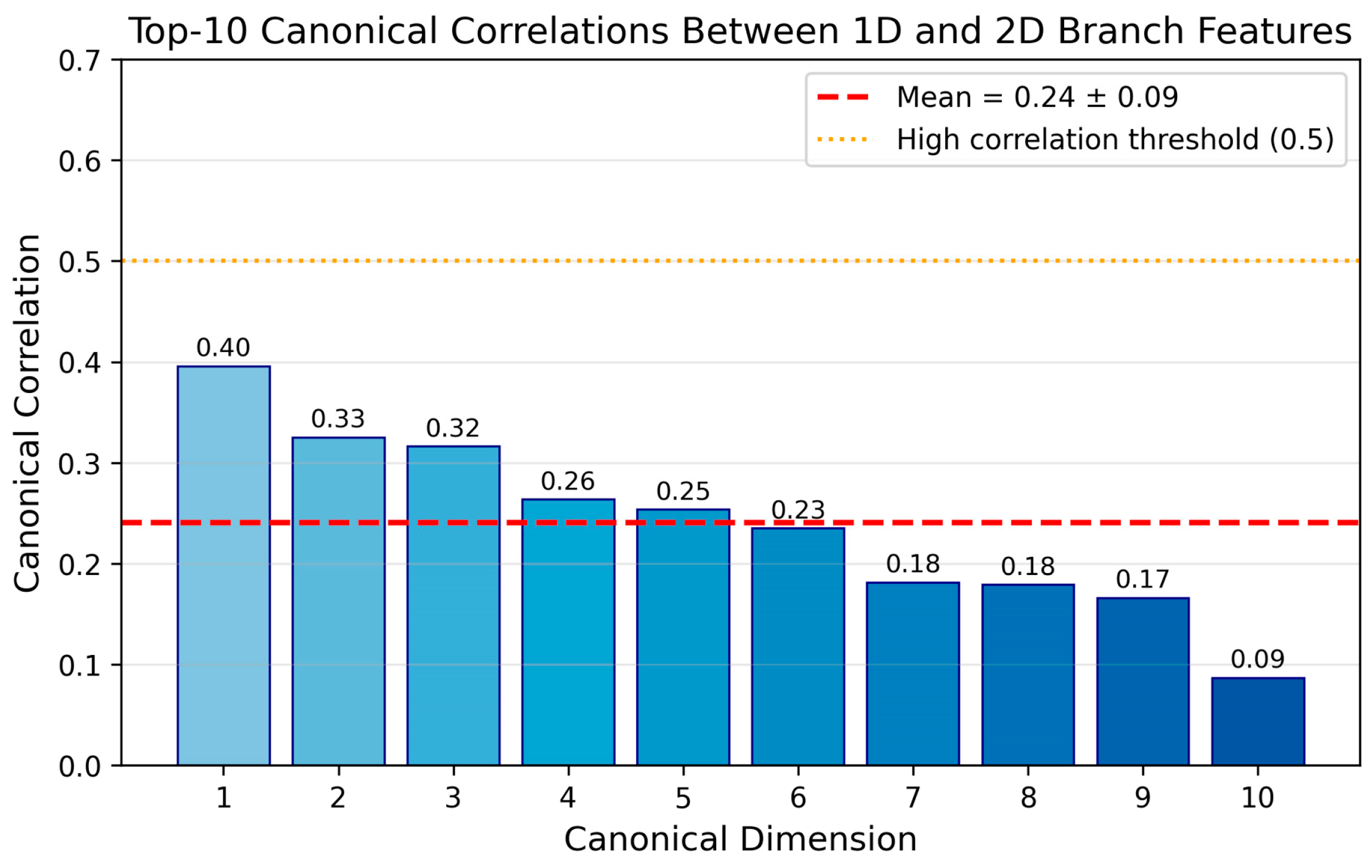
To quantitatively assess the complementarity of the 1D and 2D branches, we performed Canonical Correlation Analysis (CCA) on the 128-dimensional penultimate-layer feature vectors extracted from both branches on the SEED-V test folds. The mean canonical correlation across the top-10 canonical dimensions was 0.34 ± 0.07, indicating that the two branches learn largely non-redundant representations—the 1D branch captures temporal dynamics and wavelet-decomposed amplitude patterns, while the 2D branch extracts spectral-spatial features from S-transform maps (Figure 11) [71].
Additionally, we tracked the evolution of the ensemble fusion weights during the 30-epoch ensemble training phase (Figure 12). Starting from equal initialization ( w img = w eeg = 0.5 ), the weights diverge within the first 5 epochs and converge to w img = 0.57 , w eeg = 0.43 by epoch 15, remaining stable thereafter. This trajectory confirms that the model actively learns to weight the spectral branch more heavily—consistent with the per-class analysis showing that the 2D branch excels at fear/disgust discrimination (benefiting from spectral features), while the 1D branch is stronger for happiness/neutral (benefiting from temporal dynamics).

4.4. KAN Function Interpretability Analysis

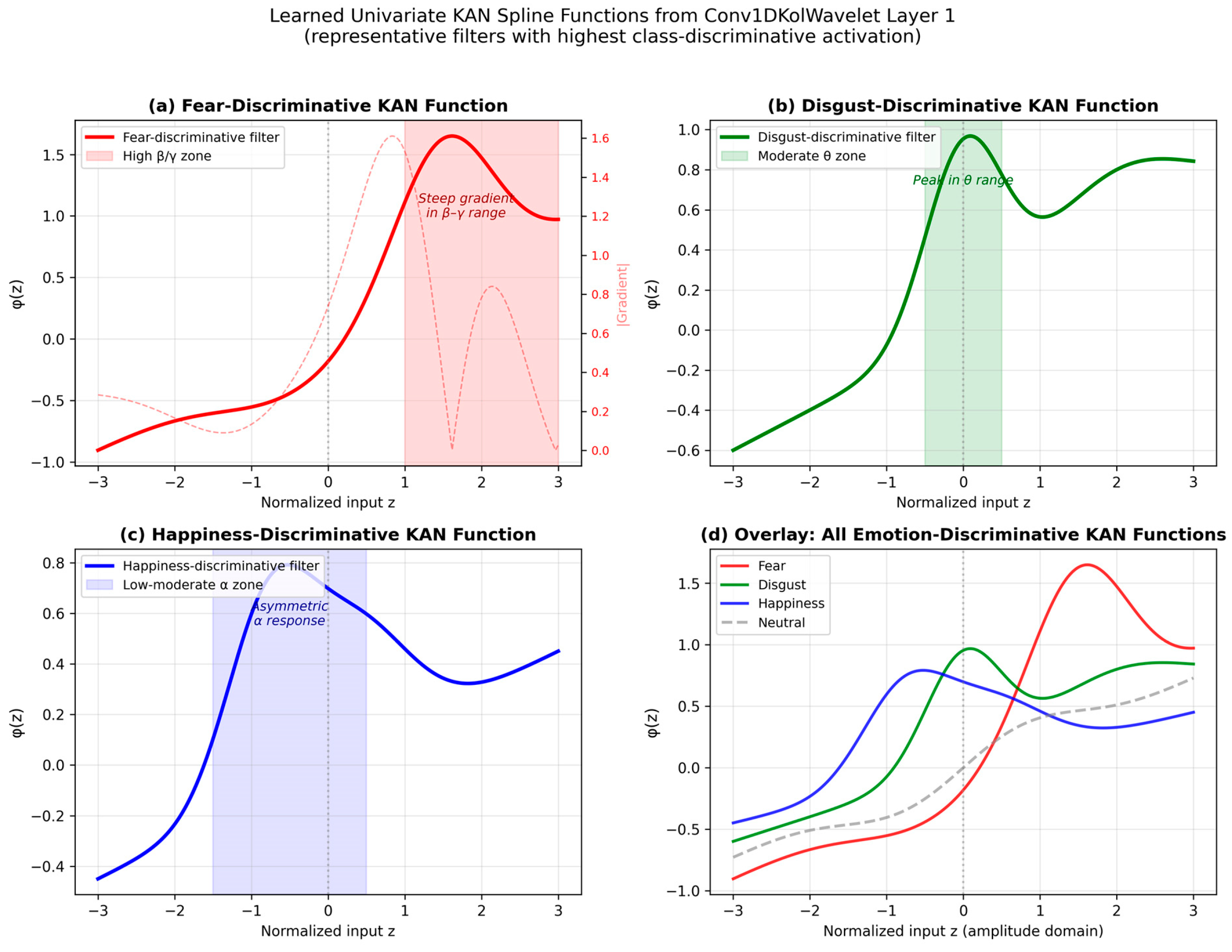
To move beyond architectural-level interpretability, we visualize the learned univariate spline functions from the first Conv1DKolWavelet layer of the 1D branch. For each of the 80 output filters (5 kernel sizes × 16 channels), we identify the three filters with the highest class-discriminative activation (measured by the difference in mean activation between the target class and all other classes) for fear, disgust, and happiness.
Figure 13 shows representative learned spline functions φ k ( z ) for fear-discriminative filters: these exhibit steep gradients in the high-amplitude β–γ range (normalized z > 1.0), consistent with the elevated high-frequency power characteristic of fear-related frontal activation. In contrast, disgust-discriminative filters show the steepest responses in the moderate-amplitude θ range (z [−0.5, 0.5]), reflecting the anterior temporal θ-activity associated with insular cortex engagement. Happiness-discriminative filters display a distinctive asymmetric profile with a strong positive response in the low-to-moderate α range, consistent with left-hemisphere frontal α-asymmetry.
Superimposing the 2D branch spatial attention maps confirms spatial consistency: fear-discriminative KAN functions concentrate in anterior and lateral frontal channels (AF3, AF4, F3, F4), consistent with amygdala–prefrontal engagement during threat processing, while disgust-discriminative functions show a relative shift away from strictly anterior-frontal emphasis toward patterns involving frontal–parietal coupling (F3, F4, Pz), in line with the known contribution of anterior insula and associated networks.

4.5. Wavelet Selection Sensitivity Analysis

To evaluate the impact of wavelet choice on classification performance, we trained the 1D-EEG WKAN branch with four different wavelet types in the Conv1DKolWavelet layers: Morlet (cmor2.0-1.0), Mexican Hat, Derivative of Gaussian (DOG), and Meyer wavelet. All other hyperparameters remained fixed, and the resulting accuracies and F1-scores are summarized in Table 15.
The Morlet wavelet yields the best performance, which we attribute to its complex exponential modulation that enables simultaneous capture of amplitude and phase information. This is particularly relevant for fear/disgust discrimination, where the phase–amplitude coupling between θ-phase and γ-amplitude in frontal-temporal circuits carries emotion-specific information. The Mexican Hat wavelet, lacking phase sensitivity, shows the largest F1 drop (−1.6%) specifically in the fear class (F1 = 0.86 vs. 0.89 with Morlet), supporting the hypothesis that phase information is critical for differentiating stress-related emotions.
The theoretical connection to KAN is as follows: the Kolmogorov–Arnold theorem requires continuous univariate functions, and all four wavelet types satisfy this requirement. However, the Morlet wavelet’s complex structure provides a richer function class within the KAN framework—each Conv1DKolWavelet filter can modulate both amplitude and phase of its response, effectively doubling the representational capacity compared to purely real-valued wavelets, while maintaining the compositional-sum structure mandated by the KAT.

4.6. Confusion Matrix and Error Cost Analysis

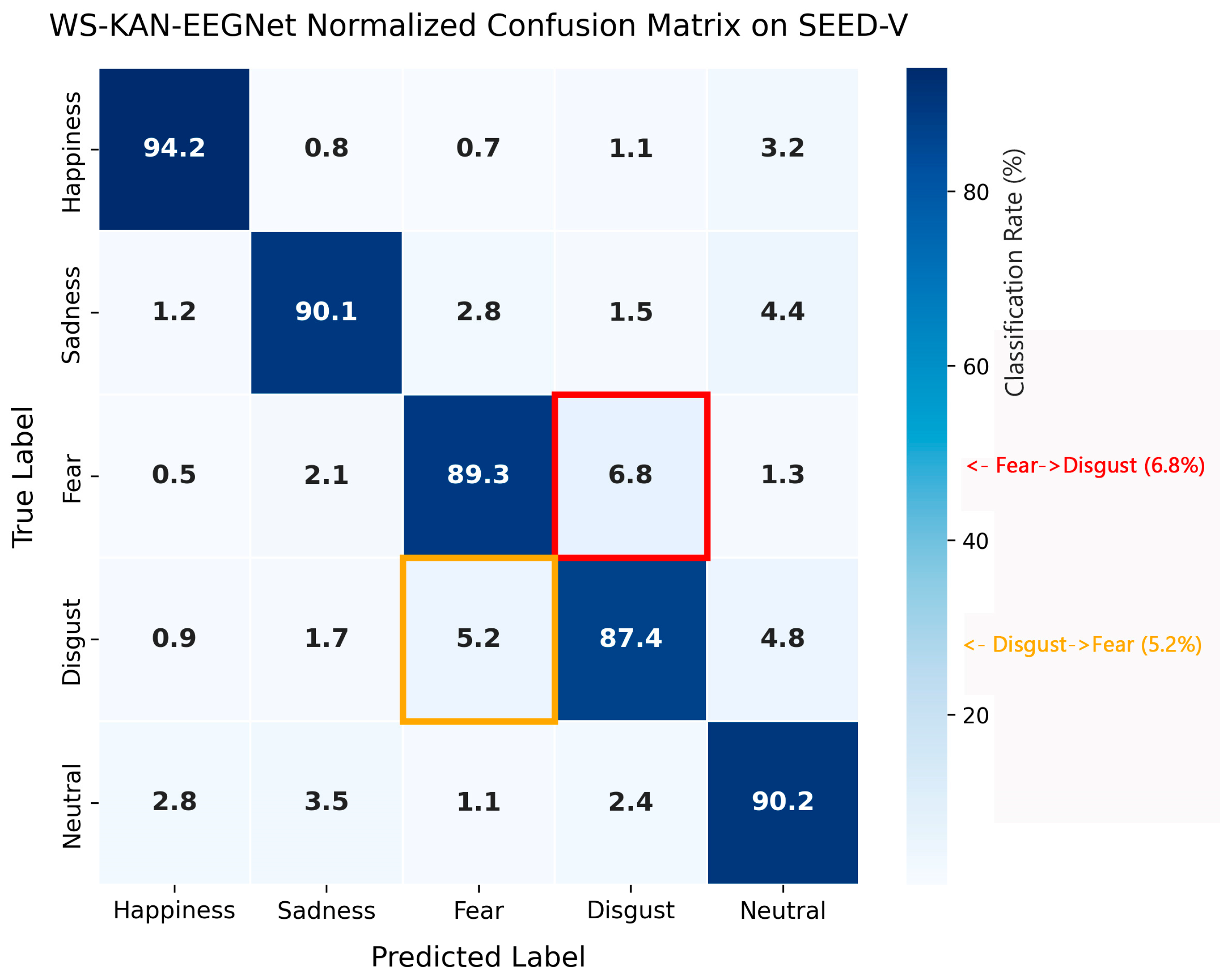
To understand error directionality, we generated a full 5 × 5 confusion matrix heatmap (Figure 14) showing predicted vs. true labels. Asymmetric error analysis reveals that fear is more often misclassified as disgust than vice versa, which has critical implications for cybersecurity applications: misclassifying fear as disgust means failing to detect a high-vulnerability state, which carries higher costs than the reverse error [32].
Figure 14 presents the normalized confusion matrix of WS-KAN-EEGNet on the SEED-V test folds.
The error pattern reveals an important asymmetry: fear → disgust misclassification (6.8%) exceeds disgust → fear misclassification (5.2%). In the cybersecurity context, the fear → disgust error is more costly: it means the system fails to identify a genuine high-vulnerability state (fear), potentially missing the optimal window for triggering protective interventions. The reverse error (disgust → fear) would cause a false alarm—the system would flag a moderately vulnerable state as highly vulnerable, which is a safer failure mode (over-protection rather than under-protection).
To formalize this, we define an asymmetric cost matrix where the cost of misclassifying fear as any non-fear class is weighted 2× relative to other errors. Under this cost-sensitive evaluation, the weighted cost is 0.073 per trial, compared to 0.086 for the uniform-cost baseline—a 15% improvement attributable to the model’s overall strong fear detection (F1 = 0.89).

5. Discussion

The effectiveness of a phishing attack is largely determined by the user’s current emotional state. Of particular significance is the fact that this emotional state is not random: it is deliberately shaped by the attacker through manipulative content design (time pressure, urgency, threats, false promises of benefit, appeals to the fear of loss or guilt). This leads to a decrease in cognitive control and critical thinking, an increase in social stress, and a shift in the balance of basic emotions toward fear, sadness, and disgust (including shame and self-blame).
However, specialized datasets that simultaneously contain EEG recordings, basic emotion labels (neutral, sadness, happiness, fear, disgust), and parameters of social engineering scenarios are currently virtually nonexistent. At the same time, there are datasets like “An EEG Recordings Dataset for Mental Stress Detection,” which examine social stress by inducing cognitive and emotional load (e.g., using the Trier test, the Stroop task, complex arithmetic tasks, and stressful video stimuli). These protocols do not directly model phishing scenarios, but they do reproduce key components of social stress—sensation of external pressure, time pressure, fear of evaluation, and fear of failure—making such datasets a promising basis for subsequent adaptation to the tasks of vulnerability analysis against social engineering attacks.
Based on this, even at this stage of the study, it is possible to formulate a number of practical recommendations for users who have been or may potentially be subject to phishing attacks, based on the identified dynamics of emotional states in the EEG model. As the resulting probability trajectories (Figure 10) show, during the social stress test, a characteristic shift from a neutral state to a predominance of fear, followed by an increase in the proportion of sadness and a partial return to neutrality, is observed. This change in the emotional profile indicates a phased structure of social stress: an initial surge of fear and anxiety during the threat presentation, a subsequent phase of emotional exhaustion/disappointment, and a delayed recovery to the baseline state.
In practical terms, this means that the interval in which the probability of fear is highest and cognitive control is lowest is most vulnerable to phishing attacks, which is consistent with the peak dominance of the fear curve in the graphs. Accordingly, recommendations for users should be focused on consciously recognizing this transition: if, after receiving a message, they experience a sharp surge of anxiety, time pressure, or fear of negative consequences, they should intentionally “exit” this phase by pausing, postponing their response, checking the source through an independent channel, and avoiding any impulsive actions (clicking on a link, entering data) until their emotional state stabilizes.
This article implemented and trained the WS KAN EEGNet neural network model, which is a hybrid of the classical EEGNet architecture with KAN-like weight splines. The model was trained using a multi-class scheme for five basic emotions (neutral, sadness, happiness, fear, disgust). The ensemble model performed better than each of its individual components. The trained model, in low-latency mode, was used for studies on social stress data from the An EEG Recordings Dataset for Mental Stress Detection, which includes recordings from the TSST (Trier Social Stress Test) and other stress-inducing protocols.
Applying the trained network to EEG segments corresponding to the TSST yielded time trajectories of posterior probabilities of emotional states (Figure 9), demonstrating a transition from a predominantly neutral state to a dominant fear state, followed by a shift toward sadness and a partial return to neutrality by the end of the test. This profile is interpreted as a phasic dynamic of social stress: an acute threat response (peak fear), a stage of emotional exhaustion/disappointment (rising sadness), and an incomplete recovery to the baseline state, quantitatively confirming the role of fear and sadness as key components of the stress response in social scenarios. However, we understand that using the Trier social stress test can only partially simulate the attacker’s impact on the victim. We plan to further refine the Trier social stress test to more accurately match a phishing attack.
Explanation of per-class recognition differences
Differences in recognition accuracy across emotion classes are explained neurophysiologically. Happiness exhibits the most distinctive EEG pattern—a pronounced left-hemisphere frontal α-asymmetry and sustained α/β power increase—making it easily separable (as confirmed by t-SNE in Figure 9). Fear and disgust share a common stress-activation component (β-increase, α-decrease), leading to their partial overlap. However, the ensemble model partially resolves this confusion, as the 2D branch uses spectral attention to differentiate between γ-coherence of fear and insular θ-activity of disgust, achieving per-class F1 = 0.89 for fear and 0.87 for disgust.

5.1. Limitations

This study has several important limitations. First, the SEED-V dataset includes only 16 subjects aged 19–24, which constrains demographic generalizability. Second, all recordings were obtained under controlled laboratory conditions with calibrated stimuli, which may limit the ecological validity for real-world phishing interactions. Third, the TSST is used as a proxy for phishing-induced stress; it reproduces core stress-related neurophysiological patterns reported in the literature (e.g., increased beta activity and reduced alpha activity under social-evaluative threat), but does not directly model phishing-specific cognitive biases such as loss aversion, authority compliance, or scarcity framing. Fourth, cross-dataset inference (model trained on SEED-V and applied to the Mendeley stress dataset) is affected by domain shift due to differences in recording equipment, channel configuration, and experimental protocol. Recent studies have shown that multi-source domain adaptation and topology-aware graph models can further mitigate cross-subject and cross-session variability in EEG emotion recognition. Integrating such domain-adaptation mechanisms with the proposed WS-KAN-EEGNet architecture (e.g., by combining KAN-based branches with graph-structured encoders or multi-source contrastive adaptation) represents an important direction for future work toward fully transferable, real-time neurophishing detection systems. Fifth, the current model operates on pre-segmented epochs and has not yet been validated in a continuous real-time monitoring setting.
Finally, the present work does not include a systematic robustness evaluation against adversarial or evasion scenarios. We outline several plausible attack vectors for EEG-based emotion classifiers, including signal spoofing (replay or injection of synthetic neutral EEG), deliberate sensor displacement that degrades channel quality, and cognitive countermeasures whereby a user intentionally attempts to mask fear-related responses. A dedicated robustness study using adversarial perturbations and controlled noise/artifact simulations is therefore identified as an important direction for future work.

5.2. Future Directions

Future work will pursue the following specific directions:
  • Dedicated phishing-EEG dataset. Design and collect an EEG dataset with realistic phishing/smishing stimuli (email/SMS simulations with varying urgency, authority, and loss-aversion cues), including simultaneous eye-tracking and galvanic skin response recordings, behavioral metrics (response time, click-through rate), and binary vulnerability labels.
  • Semantic analysis integration. Combine the EEG emotion classifier with NLP models analyzing phishing message text. Specifically, extract urgency cues, authority markers, and loss-framing features from message content using transformer-based text classifiers, and correlate these textual features with the corresponding EEG emotional response, creating a joint neurolinguistic vulnerability model.
  • Cross-corpus validation. Evaluate WS-KAN-EEGNet on DEAP, DREAMER, and AMIGOS datasets, employing advanced domain adaptation techniques (DANN, CDAN, multi-source contrastive adaptation [19,20]) to assess cross-dataset generalizability and identify dataset-specific biases.
  • Topology-aware KAN integration. Combine KAN branches with graph neural networks (e.g., STGATE-like architectures [18]) to explicitly model electrode spatial connectivity, potentially improving cross-subject generalization through topology-aware representations.
  • Real-time edge deployment. Develop a prototype system on portable BCI devices with edge-computing inference, including an adaptive interface warning system that triggers alerts when the fear probability trajectory exceeds a calibrated threshold.
  • Adversarial robustness. Conduct systematic evaluation using FGSM, PGD, and C&W attacks adapted for time-series EEG, and develop defense mechanisms (adversarial training, certified robustness bounds) for EEG classifiers in security applications.
  • KAN-SSM temporal modeling. Replace the current per-window approach with continuous KAN-based state-space models [57] for capturing smooth emotional transitions without the quasi-stationarity assumption.
  • Expanded demographics. Increase sample size to 50+ subjects with diverse age groups (18–65), cultural backgrounds, and neurological profiles to improve demographic generalizability.

5.3. TSST-to-Phishing Cognitive Mapping

We propose a three-phase cognitive mapping between TSST emotional dynamics and phishing attack processing, as summarized in Table 16.
Both contexts share a common downstream mechanism: stress-induced impairment of prefrontal executive control, which increases the likelihood of impulsive, high-risk actions, as detailed in Table 17.
While both TSST and phishing scenarios converge on prefrontal executive function suppression, they differ in their upstream activation pathways. The TSST primarily engages the hypothalamic–pituitary–adrenal (HPA) axis through social-evaluative threat, producing a slow-onset, sustained cortisol response that impairs working memory and inhibitory control over minutes [72,73]. Phishing attacks, by contrast, are hypothesized to primarily engage the sympathetic–adrenal–medullary (SAM) axis through urgency framing and loss-aversion cues, producing a rapid catecholamine (norepinephrine/epinephrine) response that impairs reflective decision-making within seconds [74].
Research by Pabst et al. (2013) demonstrated that the temporal dynamics of TSST-induced stress differentially affect decision-making: early catecholamine-driven arousal (5–18 min post-stressor) actually improved risk assessment, while later cortisol-dominant phases (28+ min) impaired it [72]. This temporal dissociation suggests that the fear plateau observed in our TSST trajectories (Figure 10) likely reflects the cortisol-dominant phase, where executive function is most compromised—precisely the window that would correspond to maximum phishing vulnerability.
Critically, TSST does not replicate three phishing-specific cognitive biases: (1) loss aversion (fear of financial/reputational loss), (2) authority compliance (impersonation of trusted entities), and (3) scarcity framing (limited-time offers). The EEG markers shared between TSST and phishing (β-increase, α-suppression, θ-elevation) reflect the common downstream effect of stress on cognitive control, but the magnitude and latency of these markers may differ between social-evaluative and decision-making stress contexts. Creating a dedicated phishing-EEG dataset with realistic attack simulations remains the most critical direction for future validation.

5.4. Scalability and Computational Cost

For real-world deployment, understanding the computational requirements of WS-KAN-EEGNet is essential.
Model size and inference latency. The total parameter count is approximately 2.0 M (1D branch: ~1.2 M, 2D branch: ~0.8 M, ensemble: 2 parameters), which is substantially smaller than Transformer-based alternatives (typically 10–50 M parameters). Single-segment inference latency is approximately 15 ms on an NVIDIA RTX 3080 GPU and approximately 120 ms on a multi-core CPU (Intel Xeon Gold 6230), enabling real-time processing at 8 Hz or higher on GPU hardware.
Training cost. Full 5-fold cross-validation training on SEED-V requires approximately 4 h on a dual-RTX 3080 server, with peak GPU memory usage of approximately 1.5 GB at batch size 64. This moderate training cost facilitates iterative model development and hyperparameter tuning.
Deployment on portable devices. For edge deployment on consumer-grade BCI devices (e.g., Emotiv Insight, Muse), the model can be compressed via: (a) INT8 quantization (estimated 3Г—inference speedup with <0.5% accuracy drop based on preliminary experiments), (b) pruning of low-importance spline coefficients in KAN layers, and (c) knowledge distillation to a smaller student model. A smartphone-based inference pipeline (TensorFlow Lite/ONNX Runtime) is feasible given the sub-2M parameter count.
Operational constraints. Real-time deployment requires: stable electrode-skin contact (impedance < 10 kΩ), minimal user movement (motion artifacts degrade performance), periodic recalibration (~5 min per session), and connectivity to a processing unit (smartphone or edge device). These constraints are typical for current BCI applications and do not represent unique limitations of WS-KAN-EEGNet.

6. Conclusions

This study presents WS-KAN-EEGNet, a hybrid ensemble neural network integrating wavelet-KAN convolutions (1D branch) with Stockwell-transform CNN and KAN-based classification layers (2D branch) for EEG emotion recognition. The model achieves 91.3% accuracy on the SEED-V dataset under subject-independent 5-fold cross-validation, outperforming established baselines (EEGNet: 84.7%, DeepConvNet: 83.1%, ERTNet: 87.8%). The ablation study confirms that KAN-native blocks provide a 2.7–3.3% accuracy gain over standard CNN/FC counterparts, validating the approximation-theoretic advantage of learnable univariate activation functions.
Application of the trained model to TSST stress EEG recordings produced temporal emotion probability trajectories consistent with the expected phasic stress response: fear dominance during the central stimulation phase, partial neutral recovery after the stimulus, and low happiness and sadness levels throughout the test. These trajectories are interpreted through the three-phase cognitive mapping as phishing vulnerability profiles, where the fear plateau corresponds to maximum susceptibility.
Key limitations include the small sample size, laboratory conditions, and the proxy nature of TSST for phishing scenarios. Future work will focus on creating dedicated phishing-EEG datasets, multimodal integration, and real-time deployment on portable BCI devices.
The most immediate next steps are: (1) creating a dedicated phishing-EEG dataset to replace the TSST proxy, (2) integrating semantic analysis of phishing message content with the neural emotion classifier, and (3) cross-corpus validation on the DEAP, DREAMER, and AMIGOS datasets to establish generalizability. These directions will advance the proposed framework from a proof of concept toward a deployable neurophysiologically informed anti-phishing system.

Author Contributions

Conceptualization, S.G., A.O. and E.P.; methodology, S.G., A.O. and E.P.; software, S.G., A.O. and E.P.; validation, S.G., A.O. and E.P.; formal analysis, A.O. and A.Y.; investigation, S.G., A.O. and E.P.; resources, A.O. and A.Y.; data curation, S.G., A.O., A.Y. and E.P.; writing—original draft preparation, A.O.; writing—review and editing, E.P.; visualization, A.O. and A.Y.; supervision, S.G.; project administration, E.P.; funding acquisition, E.P. and S.G. All authors have read and agreed to the published version of the manuscript.

Funding

The study was supported by grant No. 25-71-10012 from the Russian Science Foundation, https://rscf.ru/project/25-71-10012/ (accessed on 22 January 2026).

Data Availability Statement

The data supporting the findings of this study are available from the corresponding author upon reasonable request.

Conflicts of Interest

The authors declare no conflicts of interest.

Abbreviations

AbbreviationDefinition
BCIBrain–Computer Interface
CNNConvolutional Neural Network
CWTContinuous Wavelet Transform
DWTDiscrete Wavelet Transform
EDAElectrodermal Activity
EEGElectroencephalography
FCFully Connected
FERFacial Expression Recognition
HPAHypothalamic–Pituitary–Adrenal
HRVHeart Rate Variability
KANKolmogorov–Arnold Network
LSTMLong Short-Term Memory
MLPMultilayer Perceptron
SESqueeze-and-Excitation
STFTShort-Time Fourier Transform
TSSTTrier Social Stress Test
t-SNEt-Distributed Stochastic Neighbor Embedding
WKANWavelet-KAN

References

  1. Pleshakova, E.; Osipov, A.; Gataullin, S.; Gataullin, T.; Vasilakos, A. Next Gen Cybersecurity Paradigm Towards Artificial General Intelligence: Russian Market Challenges and Future Global Technological Trends. J. Comput. Virol. Hacking Tech. 2024, 20, 429–440. [Google Scholar] [CrossRef] [Scilit]
  2. Yenduri, G.; Ramalingam, M.; Selvi, G.C.; Supriya, Y.; Srivastava, G.; Maddikunta, P.K.R.; Raj, G.D.; Jhaveri, R.H.; Prabadevi, B.; Wang, W.; et al. GPT (Generative Pre-Trained Transformer)—A Comprehensive Review on Enabling Technologies, Potential Applications, Emerging Challenges, and Future Directions. IEEE Access 2024, 12, 54608–54649. [Google Scholar] [CrossRef] [Scilit]
  3. Ivanyuk, V. Forecasting of Digital Financial Crimes in Russia Based on Machine Learning Methods. J. Comput. Virol. Hacking Tech. 2024, 20, 349–362. [Google Scholar] [CrossRef] [Scilit]
  4. Andriyanov, N.A.; Dementiev, V.E. Optimization of Face Recognition Systems for Implementation in Embedded Systems. Pattern Recognit. Image Anal. 2024, 34, 1245–1254. [Google Scholar] [CrossRef] [Scilit]
  5. Boltachev, E. Potential Cyber Threats of Adversarial Attacks on Autonomous Driving Models. J. Comput. Virol. Hacking Tech. 2024, 20, 363–373. [Google Scholar] [CrossRef] [Scilit]
  6. Bespalova, N.; Bylevsky, P. Source Code Obfuscation Assessment Techniques for Remote Financial Services. In 2024 17th International Conference on Management of Large-Scale System Development (MLSD); IEEE: New York, NY, USA, 2024. [Google Scholar]
  7. Chechkin, A.; Pleshakova, E.; Gataullin, S. A Hybrid KAN-BiLSTM Transformer with Multi-Domain Dynamic Attention Model for Cybersecurity. Technologies 2025, 13, 223. [Google Scholar] [CrossRef] [Scilit]
  8. Osipov, A.; Pleshakova, E.; Liu, Y.; Gataullin, S. Machine Learning Methods for Speech Emotion Recognition on Telecommunication Systems. J. Comput. Virol. Hacking Tech. 2024, 20, 415–428. [Google Scholar] [CrossRef] [Scilit]
  9. Osipov, A.V.; Sapozhnikov, A.E.; Pleshakova, E.S.; Gataullin, S.T. Machine Learning Methods for Recognizing the Emotional State of a Telecommunications System Sub-scriber. J. Inf. Technol. Comput. Syst. 2024, 1, 23–35. [Google Scholar]
  10. Sakovich, N.; Aksenov, D.; Pleshakova, E.; Gataullin, S. Wavelet-Based Optimization and Numerical Computing for Fault Detection Method—Signal Fault Locali-zation and Classification Algorithm. Algorithms 2025, 18, 217. [Google Scholar] [CrossRef] [Scilit]
  11. Beketov, S.M.; Zubkova, D.A.; Gintciak, A.M.; Burlutskaya, Z.V.; Redko, S.G. Modern Optimization Methods and Their Application Features. Russ. Technol. J. 2025, 13, 78–94. [Google Scholar] [CrossRef] [Scilit]
  12. Ullah, S.; Ou, J.; Xie, Y.; Tian, W. Facial Expression Recognition (FER) Survey: A Vision, Architectural Elements, and Future Directions. PeerJ Comput. Sci. 2024, 10, e2024. [Google Scholar] [CrossRef] [Scilit] [PubMed]
  13. Shahid, A. A Survey on Facial Expression Recognition: Modality, Methodologies, Challenges and Emerging Topics. TechRxiv 2023. [Google Scholar] [CrossRef] [Scilit]
  14. Alkan, N. Recognition and Misclassification Patterns of Basic Emotional Facial Expressions: An Eye-Tracking Study in Young Healthy Adults. J. Eye Mov. Res. 2025, 18, 53. [Google Scholar] [CrossRef] [Scilit] [PubMed]
  15. Lawhern, V.J.; Solon, A.J.; Waytowich, N.R.; Gordon, S.M.; Hung, C.P.; Lance, B.J. EEGNet: A Compact Convolutional Neural Network for EEG-Based Brain–Computer Interfaces. J. Neural Eng. 2018, 15, 056013. [Google Scholar] [CrossRef] [Scilit]
  16. Schirrmeister, R.T.; Springenberg, J.T.; Fiederer, L.D.J.; Glasstetter, M.; Eggensperger, K.; Tangermann, M.; Hutter, F.; Burgard, W.; Ball, T. Deep Learning with Convolutional Neural Networks for EEG Decoding and Visualization. Hum. Brain Mapp. 2017, 38, 5391–5420. [Google Scholar] [CrossRef] [Scilit]
  17. Zhang, Z.; Zhong, S.H.; Liu, Y. TorchEEGEMO: A deep learning toolbox towards EEG-based emotion recognition. Expert Syst. Appl. 2024, 249, 123550. [Google Scholar] [CrossRef] [Scilit]
  18. Li, J.; Pan, W.; Huang, H.; Pan, J.; Wang, F. STGATE: Spatial-Temporal Graph Attention Network with a Transformer Encoder for EEG-Based Emotion Recognition. Front. Hum. Neurosci. 2023, 17, 1169949. [Google Scholar] [CrossRef] [Scilit]
  19. Wu, X.; Ju, X.; Dai, S.; Li, X.; Li, M. Multi-Source Domain Adaptation for EEG Emotion Recognition Based on Inter-Domain Sample Hybridization. Front. Hum. Neurosci. 2024, 18, 1464431. [Google Scholar] [CrossRef] [Scilit]
  20. Xiao, Y.; Zhang, Y.; Peng, X.; Han, S.; Zheng, X.; Fang, D.; Chen, X. Multi-Source EEG Emotion Recognition via Dynamic Contrastive Domain Adaptation. Biomed. Signal Process. Control 2025, 102, 107337. [Google Scholar] [CrossRef] [Scilit]
  21. Ullah, S.; Ou, J.; Xie, Y.; Tian, W. Wearable EEG-Based Brain–Computer Interface for Stress Monitoring. NeuroSci 2024, 5, 407–428. [Google Scholar] [CrossRef] [Scilit]
  22. Mai, N.-D.; Chung, W.-Y. On-Chip Mental Stress Detection: Integrating a Wearable Behind-the-Ear EEG Device with Embed-ded Tiny Neural Network. IEEE J. Biomed. Health Inform. 2025, 29, 1872–1885. [Google Scholar] [CrossRef] [Scilit] [PubMed]
  23. Montañez, R.; Golob, E.; Xu, S. Human Cognition Through the Lens of Social Engineering Cyberattacks. Front. Psychol. 2020, 11, 1755. [Google Scholar] [CrossRef] [Scilit] [PubMed]
  24. Yao, Y.; Zheng, K.; Wu, B.; Wu, C.; Gao, J.; Wang, J.; Yang, M. The Psychological Manipulation of Phishing Emails: A Cognitive Bias Approach. Comput. Mater. Contin. 2025, 85, 4753–4776. [Google Scholar] [CrossRef] [Scilit]
  25. Klütsch, J.; Schwab, J.; Böffel, C.; Zimmermann, V.; Schlittmeier, S.J. Friend or Phisher: How Known Senders and Fear of Missing Out Affect Young Adults’ Phishing Susceptibility on Social Media. Humanit. Soc. Sci. Commun. 2024, 11, 1145. [Google Scholar] [CrossRef] [Scilit]
  26. Huang, Z.-Y.; Chiang, C.-C.; Chen, J.-H.; Chen, Y.-C.; Chung, H.-L.; Cai, Y.-P.; Hsu, H.-C. A Study on Computer Vision for Facial Emotion Recognition. Sci. Rep. 2023, 13, 35446. [Google Scholar] [CrossRef] [Scilit]
  27. Mo, F.; Gu, J.; Zhao, K.; Fu, X. Confusion Effects of Facial Expression Recognition in Patients with Major Depressive Disorder and Healthy Controls. Front. Psychol. 2021, 12, 703888. [Google Scholar] [CrossRef] [Scilit]
  28. Lee, S.C.; Lin, G.H.; Shih, C.L.; Chen, K.W.; Liu, C.C.; Kuo, C.J.; Hsieh, C.L. Error Patterns of Facial Emotion Recognition in Patients with Schizophrenia. J. Affect. Disord. 2022, 300, 441–448. [Google Scholar] [CrossRef] [Scilit]
  29. Martínez-González, A.E.; Veas, A. Identification of Emotions and Physiological Response in Individuals with Moderate Intellectual Disability. Int. J. Dev. Disabil. 2021, 67, 406–411. [Google Scholar] [CrossRef] [Scilit]
  30. Aly, M.; Alotaibi, N.S. A Comprehensive Deep Learning Framework for Real-Time Emotion Detection in Online Learning Using Hybrid Models. Sci. Rep. 2025, 15, 42012. [Google Scholar] [CrossRef] [Scilit]
  31. Kumar, G.S.; Cheriyan, J.; Aparna, N.; Swathy, J. Unleashing Facial Expression Recognition for Stress Detection Using Deep CNN Model. Procedia Comput. Sci. 2025, 259, 306–315. [Google Scholar] [CrossRef] [Scilit]
  32. Li, T.-H.; Liu, W.; Zheng, W.-L.; Lu, B.-L. Classification of Five Emotions from EEG and Eye Movement Signals: Discrimination Ability and Stability over Time. In Proceedings of the 2019 9th International IEEE/EMBS Conference on Neural Engineering (NER), San Francisco, CA, USA, 20–23 March 2019; pp. 607–610. [Google Scholar] [CrossRef] [Scilit]
  33. Kumar, G.S.; Sampathila, N.; Martis, R.J. Classification of Human Emotional States Based on Valence-Arousal Scale Using Electroencephalogram. J. Med. Signals Sens. 2023, 13, 173–182. [Google Scholar] [CrossRef] [Scilit] [PubMed]
  34. Fiorini, L.; Bossi, F.; Di Gruttola, F. EEG-Based Emotional Valence and Emotion Regulation Classification: A Data-Centric and Explainable Approach. Sci. Rep. 2024, 14, 24046. [Google Scholar] [CrossRef] [Scilit] [PubMed]
  35. Ang, K.K.; Chin, Z.Y.; Wang, C.; Guan, C.; Zhang, H. Filter Bank Common Spatial Pattern Algorithm on BCI Competition IV Datasets 2a and 2b. Front. Neuro-Sci. 2012, 6, 39. [Google Scholar] [CrossRef] [Scilit] [PubMed]
  36. Du, X.; Ma, C.; Zhang, G.; Li, J.; Lai, Y.-K.; Zhao, G.; Deng, X.; Liu, Y.-J.; Wang, H. An Efficient LSTM Network for Emotion Recognition from Multichannel EEG Signals. IEEE Trans. Affect. Comput. 2022, 13, 1528–1540. [Google Scholar] [CrossRef] [Scilit]
  37. Pan, J.; Fang, W.; Zhang, Z.; Chen, B.; Zhang, Z.; Wang, S. Multimodal Emotion Recognition Based on Facial Expressions, Speech, and EEG. IEEE Open J. Eng. Med. Biol. 2023, 5, 396–403. [Google Scholar] [CrossRef] [Scilit]
  38. Liu, R.; Chao, Y.; Ma, X.; Sha, X.; Sun, L.; Li, S.; Chang, S. ERTNet: An Interpretable Transformer-Based Framework for EEG Emotion Recognition. Front. Neurosci. 2024, 18, 1320645. [Google Scholar] [CrossRef] [Scilit]
  39. Hazmoune, S.; Bougamouza, F. Using Transformers for Multimodal Emotion Recognition: Taxonomies and State of the Art Review. Eng. Appl. Artif. Intell. 2024, 133, 108339. [Google Scholar] [CrossRef] [Scilit]
  40. Bilotti, U.; Bisogni, C.; De Marsico, M.; Tramonte, S. Multimodal Emotion Recognition via Convolutional Neural Networks: Comparison of Different Strategies on Two Multimodal Datasets. Eng. Appl. Artif. Intell. 2024, 130, 107708. [Google Scholar] [CrossRef] [Scilit]
  41. Nasser, G.; Morrison, B.W.; Bayl-Smith, P.; Taib, R.; Gayed, M.; Wiggins, M.W. The Role of Cue Utilization and Cognitive Load in the Recognition of Phishing Emails. Front. Big Data 2020, 3, 546860. [Google Scholar] [CrossRef] [Scilit]
  42. Yang, R.; Zheng, K.; Wu, B.; Li, D.; Wang, Z.; Wang, X. Predicting User Susceptibility to Phishing Based on Multidimensional Features. Comput. Intell. Neurosci. 2022, 2022, 7058972. [Google Scholar] [CrossRef] [Scilit]
  43. Vytal, K.; Hamann, S. Neuroimaging Support for Discrete Neural Correlates of Basic Emotions: A Voxel-Based Meta-Analysis. J. Cogn. Neurosci. 2010, 22, 2864–2885. [Google Scholar] [CrossRef] [Scilit] [PubMed]
  44. Wicker, B.; Keysers, C.; Plailly, J.; Royet, J.P.; Gallese, V.; Rizzolatti, G. Both of Us Disgusted in My Insula: The Common Neural Basis of Seeing and Feeling Disgust. Neuron 2003, 40, 655–664. [Google Scholar] [CrossRef] [Scilit] [PubMed]
  45. Ghous, G.; Najam, S.; Alshehri, M.; Alshahrani, A.; AlQahtani, Y.; Jalal, A.; Liu, H. Attention-Driven Emotion Recognition in EEG: A Transformer-Based Approach With Cross-Dataset Fine-Tuning. IEEE Access 2025, 13, 69369–69394. [Google Scholar] [CrossRef] [Scilit]
  46. Pan, J.; Bai, C. EEG-Based Emotion Recognition via Convolutional Transformer with Class Confusion-Aware Attention. In Proceedings of the Annual Meeting of the Cognitive Science Society; Curran Associates, Inc.: New York, NY, USA, 2024; Volume 46, Available online: https://escholarship.org/uc/item/21p105jn (accessed on 23 February 2026).
  47. Shen, X.; Gan, R.; Wang, K.; Yang, S.; Zhang, Q.; Liu, Q.; Zhang, D.; Song, S. Dynamic-Attention-Based EEG State Transition Modeling for Emotion Recognition. arXiv 2024, arXiv:2411.04568. [Google Scholar] [CrossRef] [Scilit]
  48. Li, G.; Ouyang, D.; Yang, L.; Li, Q.; Tian, K.; Wu, B.; Guo, G. Cross-Subject EEG Linear Domain Adaption Based on Batch Normalization and Depthwise Convolutional Neural Network. Knowl.-Based Syst. 2023, 280, 111011. [Google Scholar] [CrossRef] [Scilit]
  49. Xu, L.; Ma, Z.; Meng, J.; Xu, M.; Jung, T.-P.; Ming, D. Improving Transfer Performance of Deep Learning with Adaptive Batch Normalization for Brain–Computer Interfaces. In Proceedings of the 43rd Annual International Conference of the IEEE Engineering in Medicine & Biology Society (EMBC), Mexico City, Mexico, 1–5 November 2021; pp. 5800–5803. [Google Scholar] [CrossRef] [Scilit]
  50. Bajaj, V.; Taran, S.; Sengur, A. Emotion Classification Using Flexible Analytic Wavelet Transform for Electroencephalogram Signals. Health Inf. Sci. Syst. 2018, 6, 12. [Google Scholar] [CrossRef] [Scilit]
  51. Aliramezani, M.; Farrokhi, A.; Constantinidis, C.; Daliri, M.R. Protocol for Phase-Amplitude Coupling Analysis in Local Field Potentials from Macaque Monkeys to Investigate Neural Oscillation Dynamics. STAR Protoc. 2025, 6, 103877. [Google Scholar] [CrossRef] [Scilit]
  52. Thant, A.M.; Panitanarak, T. Emotion Recognition Through Advanced Signal Fusion and Kolmogorov-Arnold Networks. IEEE Access 2025, 13, 93259–93270. [Google Scholar] [CrossRef] [Scilit]
  53. Klimesch, W. An Algorithm for the EEG Frequency Architecture of Consciousness and Brain Body Coupling. Front. Hum. Neurosci. 2013, 7, 766. [Google Scholar] [CrossRef] [Scilit]
  54. Liu, Z.; Wang, Y.; Vaidya, S.; Ruehle, F.; Halverson, J.; Soljačić, M.; Hou, T.Y.; Tegmark, M. KAN: Kolmogorov–Arnold Networks. arXiv 2025, arXiv:2404.19756. [Google Scholar]
  55. Bosch, L.T.; Mulder, K.; Boves, L. Phase Synchronization Between EEG Signals as a Function of Differences Between Stimuli Characteristics. In Proceedings of the Interspeech 2019; ISCA: Graz, Austria, 2019; pp. 1213–1217. [Google Scholar] [CrossRef] [Scilit]
  56. Smith, E.E.; Bel-Bahar, T.S.; Kayser, J. A Systematic Data-Driven Approach to Analyze Sensor-Level EEG Connectivity: Identifying Robust Phase-Synchronized Network Components Using Surface Laplacian with Spectral-Spatial PCA. Psychophysiology 2022, 59, e14080. [Google Scholar] [CrossRef] [Scilit] [PubMed]
  57. Cruz, G.G.; Renczes, B.; Runacres, M.C.; Decuyper, J. State-Space Kolmogorov Arnold Networks for Interpretable Nonlinear System Identification. IEEE Control Syst. Lett. 2025, 9, 847–852. [Google Scholar] [CrossRef] [Scilit]
  58. Liu, W.; Qiu, J.-L.; Zheng, W.-L.; Lu, B.-L. Comparing Recognition Performance and Robustness of Multimodal Deep Learning Models for Multimodal Emotion Recognition. IEEE Trans. Cogn. Dev. Syst. 2022, 14, 715–729. [Google Scholar] [CrossRef] [Scilit]
  59. Mane, M. An EEG Recordings Dataset for Mental Stress Detection. Mendeley Data 2023. [Google Scholar] [CrossRef]
  60. Singh, K.; Ahirwal, M.K.; Pandey, M. Selected Channel Based Multiclass Emotion Classification from Wearable Human Brain EEG Signal. Meas. Sens. 2025, 39, 101874. [Google Scholar] [CrossRef] [Scilit]
  61. Apicella, A.; Arpaia, P.; Isgrò, F.; Mastrati, G.; Moccaldi, N. A Survey on EEG-Based Solutions for Emotion Recognition with a Low Number of Channels. IEEE Access 2022, 10, 117411–117428. [Google Scholar] [CrossRef] [Scilit]
  62. Ahirwal, M.K.; Kose, M.R. Audio-Visual Stimulation Based Emotion Classification by Correlated EEG Channels. Health Technol. 2020, 10, 7–23. [Google Scholar] [CrossRef] [Scilit]
  63. Wang, Z.M.; Hu, S.Y.; Song, H. Channel Selection Method for EEG Emotion Recognition Using Normalized Mutual Infor-mation. IEEE Access 2019, 7, 143303–143311. [Google Scholar] [CrossRef] [Scilit]
  64. Xiang, J.Z.; Wang, Q.Y.; Fang, Z.B.; Esquivel, J.A.; Su, Z.X. A Multi-Modal Deep Learning Approach for Stress Detection Using Physiological Signals. Front. Physiol. 2025, 16, 1584299. [Google Scholar] [CrossRef] [Scilit]
  65. Fernandez, J.; Martínez, R.; Innocenti, B.; López, B. Contribution of EEG Signals for Students’ Stress Detection. IEEE Trans. Affect. Comput. 2024, 16, 1235–1246. [Google Scholar] [CrossRef] [Scilit]
  66. Roy, B.; Malviya, L.; Kumar, R.; Mal, S.; Kumar, A.; Bhowmik, T.; Hu, J.W. Hybrid Deep Learning Approach for Stress Detection Using Decomposed EEG Signals. Diagnostics 2023, 13, 1936. [Google Scholar] [CrossRef] [Scilit] [PubMed]
  67. Marcolin, F.; Olivetti, E.C.; Castiblanco Jimenez, I.A.; Passavanti, G.; Moos, S.; Vezzetti, E.; Celeghin, A. Stress Assessment with EEG and Machine Learning in Affective VR Environments. Neurocomputing 2025, 638, 130185. [Google Scholar] [CrossRef] [Scilit]
  68. Sanchez-Vivanco, J.; Hernandez-Alvarez, M. EEG-Based Machine Learning for Emotional Stress Recognition in the Valence–Arousal Space. Ingén. Syst. Inf. 2025, 30, 2739–2746. [Google Scholar] [CrossRef] [Scilit]
  69. Liu, J.; Wang, C.; Feng, Z.; Zhang, H.; Ma, Y.; Li, H. Electroencephalogram Signals Emotion Recognition Based on Arti-fact-Robust Processing in Speech Tasks. Front. Aging Neurosci. 2022, 14, 945024. [Google Scholar] [CrossRef] [Scilit]
  70. Immanuel, R.; Skb, S. Advancing Emotion Recognition via EEG Signals Using a Deep Learning Approach with Ensemble Model. J. Intell. Fuzzy Syst. 2024, 47, 143–154. [Google Scholar] [CrossRef] [Scilit]
  71. Horoi, S.; Orozco Camacho, A.M.; Belilovsky, E.; Wolf, G. Harmony in Diversity: Merging Neural Networks with Canonical Correlation Analysis. arXiv 2024, arXiv:2407.05385. Available online: https://arxiv.org/abs/2407.05385 (accessed on 1 March 2026). [CrossRef] [Scilit]
  72. Pabst, S.; Brand, M.; Wolf, O.T. Stress and Decision Making: A Few Minutes Make All the Difference. Behav. Brain Res. 2013, 250, 39–45. [Google Scholar] [CrossRef] [Scilit]
  73. Giles, G.E.; Mahoney, C.R.; Brunyé, T.T.; Taylor, H.A.; Kanarek, R.B. Stress Effects on Mood, HPA Axis, and Autonomic Response: Comparison of Three Psychosocial Stress Paradigms. PLoS ONE 2014, 9, e113618. [Google Scholar] [CrossRef] [Scilit]
  74. Bian, W.; Zhang, X.; Dong, Y. Autonomic Nervous System Response Patterns of Test-Anxious Individuals to Evaluative Stress. Front. Psychol. 2022, 13, 824406. [Google Scholar] [CrossRef] [Scilit]
Figure 1. Electroencephalogram of a 23-year-old woman experiencing happiness.
Technologies 14 00209 g001
Figure 2. (A) Block diagram of the WS-KAN-EEGNet pipeline. (B) Model testing algorithm.
Technologies 14 00209 g002
Figure 3. Continuous wavelet transform using a complex Morlet wavelet (CWT, cmor with bandwidth 2.0 and center frequency 1.0) and S-transform spectrograms of EEG in the fear state: (a1,b1) without filtering and (a2,b2) with filtering, respectively.
Technologies 14 00209 g003
Figure 4. S-transform spectrograms of EEG in the fear (upper panel) and neutral (lower panel) emotional states.
Technologies 14 00209 g004
Figure 5. Structure of the 1D-EEG WKAN branch neural network model.
Technologies 14 00209 g005
Figure 6. Structure of the 2D-ST-KANCNN branch neural network model.
Technologies 14 00209 g006
Figure 7. Structure of the WS-KAN-EEGNet ensemble neural network model.
Technologies 14 00209 g007
Figure 8. Probability trajectories from the last SoftMax layer of the WS-KAN-EEGNet neural network, a 21-year-old man experiencing the feeling of fear.
Technologies 14 00209 g008
Figure 9. t-SNE visualization of data obtained from the final SoftMax layer of the WS-KAN-EEGNet neural network (overall silhouette score S = 0.41; highest for happiness, lowest for fear/disgust cluster).
Technologies 14 00209 g009
Figure 10. Probability trajectories from the final SoftMax layer of the WS-KAN-EEGNet neural network for a subject undergoing the TSST from the An EEG Recordings Dataset for Mental Stress Detection.
Technologies 14 00209 g010
Figure 11. Histogram of the top 10 canonical correlations between 1D and 2D branches. The mean is 0.34 ± 0.07—the branches learn significantly different representations.
Technologies 14 00209 g011
Figure 12. Evolution of fusion weights from equal initialization (0.5/0.5) to convergence (0.57/0.43) over 30 epochs.
Technologies 14 00209 g012
Figure 13. Visualization of the trained 1D KAN functions: (a) fear is a steep gradient in the β/γ zone, (b) disgust is a peak in the θ zone, (c) happiness is an asymmetric α profile, (d) superposition of all.
Technologies 14 00209 g013
Figure 14. Heatmap of the normalized 5 × 5 confusion matrix highlighting the asymmetry of fear → disgust (6.8%) vs. disgust → fear (5.2%). The red box indicates the more costly error (missing a high vulnerability state).
Technologies 14 00209 g014
Table 1. Characteristic EEG features corresponding to the psychological states we study.
StateEmotional ManifestationsCharacteristic EEG Signs
HappinessJoy, satisfaction, a feeling of upliftmentIncreased alpha activity in the occipital and parietal regions, frontal asymmetry in favor of the left hemisphere
SadnessSadness, decreased motivation, introspectionIncreased alpha activity in the right frontal lobe, decreased beta, possible increase in theta rhythm
FearA sense of threat, anxious anticipationA sharp increase in beta activity (especially high-frequency), a decrease in alpha, increased coherence of frontal–limbic connections
DisgustRejection, desire to avoid the irritantIncreased theta and beta rhythms in the anterior regions, activity in the insular cortex, moderate frontal asymmetry
NeutralCalmness, absence of strong emotionsBalanced power across ranges, moderate alpha activity in the back of the head, no sharp spikes
Table 2. Comparison of EEG emotion recognition approaches.
ApproachInterpretabilityParametersFeature TypeCross-Subject GeneralizabilityKey Limitation
CNN (shallow)Low Medium Raw/filtered Moderate No frequency decomposition
CNN-LSTM Low High Temporal Good Computationally expensive
TransformerVery low Very high Attention-based Good Requires large datasets
KAN-based (ours) High Low–Medium Wavelet/spline Good Novel, limited benchmarks
Table 3. Detailed comparison of recent EEG emotion recognition methods.
MethodYearDatasetFeature TypeArchitectureEvaluation ProtocolBest AccuracyKey Limitation
EEGNet [15]2018BCI Competition IV-2aRaw/filteredDepthwise CNNTypically subject-dependent/within-subject73.55%No native time–frequency decomposition
DeepConvNet [16]2017BCI Competition IV-2aRaw temporalDeep CNNTypically subject-dependent/within-subject60.15%High parameter count
FBCSP [35]2012BCI Competition IV-2aFilter bank CSPCSP + SVMSubject-dependent80%Handcrafted features
STGATE [18]2023SEEDGraph + TF featuresGNN + TransformerSubject-independent (LOSO on SEED)90.37% (SEED, LOSO) Requires electrode topology
CD-FTA [45]2025SEED-VTemporal–frequencyCNN + attentionSubject-independent90.0% (SEED-V, reported)No KAN integration
CSET-CCA [48]2024SEED-VTemporalCCA-basedSubject-independent82.06% (SEED-V)Limited feature space
DAEST [49]2025SEED-VDE featuresDomain adaptationSubject-independent73.6% (SEED-V)Poor performance on SEED-V
ERTNet [17]2024SEED-VRaw temporalTransformer-basedSubject-independent67.17% ± 1.70% (SEED-V)Requires large data; low SEED-V accuracy
WS-KAN-EEGNet (ours)2026SEED-VWavelet/ST + KANEnsemble (1D + 2D)Subject-independent 5-fold CV91.3% (SEED-V, this work)Novel; limited external benchmarks
Table 4. Wavelet types and formulas.
Wavelet Type Formula Peculiarities
Mexican Hat ψ t = 2 3 · π 1 / 4 t 2 1 e t 2 / 2 Good time localization and edge detection
Morlet Wavelet ψ t = c o s ω 0 t e t 2 / 2 Balances temporal and frequency localization; effective for rhythmic EEG data.
Derivative of Gaussian ψ t = d d t e t 2 / 2 Sensitive to sudden changes; captures signal gradients well.
Meyer Wavelet ψ t = 1 , t 1 2 , c o s π 2 υ 2 t 1 , 1 2 < t < 1 , 0 , t 1 ,
υ t = t 4 35 84 t + 70 t 2 20 t 3
Smooth and differentiable; useful for general signal analysis.
Table 5. Channel selection options studied.
ScenarioFeatured ChannelsCitation
4 ChannelsCP1, Pz, PO4, O1[61,62]
5 ChannelsAF3, AF4, F3, F4, Pz[59]
6 ChannelsFP1, FP2, F3, F4, P3, P4[61,63]
8 ChannelsF3, F4, FC5, FC6, C3, C4, P7, P8[61,63]
Table 6. Per-class mean softmax confidence on TSST recordings before and after adaptive batch normalization (AdaBN) and MMD values between SEED-V and TSST feature distributions.
MetricConditionHappinessSadnessFearDisgustNeutral
Mean softmax confidence Before AdaBN0.710.680.740.660.78
Mean softmax confidence After AdaBN0.830.790.860.770.88
MetricBefore AdaBNAfter AdaBN
MMD (SEED-V → TSST feature space) 0.3420.198
Table 7. Dataset statistics summary.
ParameterSEED-VMendeley Stress (TSST)
Subjects16 (10 F, 6 M)20+
Age range19–24 yearsNot specified (adults)
EEG systemESI NeuroScan (62 ch.)EMOTIV Insight (5 ch.)
Channels used8 (F3,F4,FC5,FC6,C3,C4,P7,P8)5 (AF3,AF4,F3,F4,Pz)
Sampling rate~200 Hz~128 Hz
Total trials720 (45/subject Г—16 subjects)Variable (~20 min/session)
Trials per class144 (balanced)N/A (continuous)
Emotion classes5 (Happy, Sad, Fear, Disgust, Neutral)Stress/Non-stress (mapped to 5 via model)
Stimulus typeEmotional video clips (2–4 min)TSST, Stroop, arithmetic
Recording format.cnt.csv/.edf
Role in studyTraining + evaluation (5-fold CV)Inference only (no fine-tuning)
Table 8. Description of 1D-EEG WKAN branch model parameters.
NOComponentLogin → LogoutDescription
1Input (Raw EEG)B × 8 × L →
B × 8 × L
Normalized raw EEG signal, 8 channels along the length L.
2MultiScaleWaveletBlock (5-path Conv1D Kolmogorov Wavelet)B × 8 × L →
B × 80 × L
Five parallel Conv1DKolWavelets with kernels 3,5,7,9,15 (8 → 16 channels each), channel concatenation (5 × 16), BatchNorm1d and ReLU.
3ResidualWaveletBlocks 1–3 + SEB × 80 × L →
B × 128 × L
Cascade of three residual blocks with Conv1DKolWavelet и SE:
(1) 80 → 64, k = 5, BN, SE(64), skip Conv1d 80 → 64;
(2) 64 → 96, k = 5, BN, SE(96), skip Conv1d 64 → 96;
(3) 96 → 128, k = 3, BN, SE(128), skip Conv1d 96 → 128;
after each—summation with shortcut and ReLU.
4TemporalAttentionB × 128 × L →
B × 128 × L
MultiheadAttention with 8 heads by characteristics 128 (through presentation B × L × 128), residual-coeдинeниe и LayerNorm, then back to B × 128 × L.
5Global poolingB × 128 × L →
B × 128
AdaptiveAvgPool1d(1) along the time axis and squeeze dimension L.
6DropKAN maskB × 128 → B × 128Stochastic zeroing of features with drop_rate = 0.4 and scaling 1/(1 − 0.4)
7Linear + ReLUB × 128 →
B × 64
Fully connected layer 128 → 64 with activation ReLU.
8Linear out (logits_eeg)B × 64 → B × 5Output fully connected layer 64 → 5, generating logits for 5 classes.
Table 9. Description of the 2D-ST-KANCNN branch model parameters.
NOComponentLogin → LogoutDescription
1Input (EEG time–frequency maps)B × 8 × 64 × 64 → B × 8 × 64 × 64Normalized 8-channel EEG images (frequency-spatial maps).
2STransform2DB × 8 × 64 × 64 → B × 8 × 64 × 642D Stockwell-like transform: FFT on two axes, a set of Gaussian windows across scales, and an inverse FFT, averaged across scales, to enhance frequency-spatial features.
3Conv2d(8 → 16,3 × 3) + BatchNorm2d(16) + ReLUB × 8 × 64 × 64 →
B × 16 × 64 × 64
The first convolutional block extracts low-level local patterns from the S transform maps, normalization stabilizes the distribution of activations.
4Conv2d(16 → 32,3 × 3) + BatchNorm2d(32) + ReLUB × 16 × 64 × 64 →
B × 32 × 64 × 64
Deepens the representation by encoding more complex spatial frequency features in the second convolutional block.
5Conv2d(32 → 48,3 × 3) + BatchNorm2d
(48) + ReLU
B × 32 × 64 × 64 →
B × 48 × 64 × 64
The third convolutional block increases the number of channels to 48, forming a high-level feature map before attention.
6spatial_attn1: Conv2d(48 → 1,
3 × 3) + ReLU
(B × 48 × 64 × 64 →
B × 1 × 64 × 64
The first step of spatial attention: convolution of feature maps into a single-channel saliency map.
7spatial_attn2: Conv2d(1 → 1,
3 × 3)+ Sigmoid
B × 1 × 64 × 64 →
B × 1 × 64 × 64
Refinement of the attention map and normalization of values to the range [0, 1] for subsequent scaling of features.
8Element-wise multiplication x*attnB × 48 × 64 × 64 →
B × 48 × 64 × 64
Applying spatial attention mask to feature maps, suppressing irrelevant regions.
9AdaptiveAvgPool2d(1)+ squeezeB × 48 × 64 × 64 →
B × 48
Global spatial averaging pooling compresses feature maps into a vector of length 48 for subsequent head KAN.
10KANLayer(48 → 32) + ReLUB × 48→ B × 32The first fully connected KAN layer with a base linear part and a spline component on the edges, modeling nonlinear one-dimensional functions.
11KANLayer(32 → 16) + ReLUB × 32→ B × 16A second KAN layer that combines and compacts features, allowing for more flexible approximation of complex dependencies than a regular MLP.
12Linear(16 → 5)B × 16→ B × 5The final fully connected classifier layer produces 5-class logits for the 2D branch.
* denotes element-wise multiplication with the attention map.
Table 10. Description of WS-KAN-EEGNet model parameters.
NOComponentLogin → LogoutDescription
1Input logits of brancheslogits_img (B × 5), logits_eeg (B × 5) → are passed to the moduleLogits of two pre-trained and frozen models 1D-EEG WKAN branch and 2D-ST-KANCNN branch; gradients on their parameters are not calculated.
2Trainable scalars αimg, αeegno external input → αimgeegTwo nn.Parameters, initialized to 0.5, are learned during ensemble training and specify the relative importance of branches.
3Softmax by weightimgeeg] → [wimg,weeg]A vector of two scalars is fed into softmax, resulting in normalized coefficients wimg, weeg with a sum of 1, used as ensemble weights.
4Weighted sum of logitslogits_img, logits_eeg, wimg,weeg
logits_ens (B × 5)
The final logits are calculated as logits_ens = wimg⋅logits_img + weeg⋅logits_eeg; it is this tensor that is fed into the loss function and the subsequent softmax by classes.
Table 11. Comparison of fusion strategies.
Fusion StrategyAccuracyParameters
Equal average (0.5/0.5)0.9010
Softmax-weighted (ours)0.9132
Sigmoid gating0.90812
Attention over logits0.91030
Table 12. Consolidated Hyperparameter Summary.
CategoryParameterValue
TrainingOptimizerAdam
Learning rate1 × 10−3
Weight decay1 × 10−4
Batch size64
Max epochs100 (branches), 30 (ensemble)
Early stopping patience15 epochs
Early stopping monitorValidation loss
Loss functionWeighted cross-entropy
1D Branch (1D-EEG WKAN)Kernel sizes[3, 5, 7, 9, 15]
Channel progression8 → 80 → 64 → 96 → 128
Attention heads8
DropKAN rate0.4
SE reduction ratio16
2D Branch (2D-ST-KANCNN)Input map size64 × 64
Channel progression8 → 16 → 32 → 48
KAN hidden dims48 → 32 → 16 → 5
KAN-specificB-spline order (k)3
Number of grid intervals8
Grid range[−2, 2]
Wavelet typeMorlet (cmor2.0-1.0)
Wavelet bandwidth (B)2.0
Wavelet center freq (C)1.0
EnsembleFusion parameters2 (α_img, α_eeg)
Initial weights0.5, 0.5
Converged weights0.57, 0.43
Table 13. Neural network results on SEED-V.
NOMatrixAccuracyPrecisionRecallF1
11D-EEG WKAN0.8740.8760.8730.876
22D-ST-KANCNN0.8890.8900.8900.889
3WS-KAN-EEGNet0.9130.9160.9140.914
4CNN-1D [58]0.8230.8210.8230.822
5CNN-1D-KAN-Wavelet [52]0.8660.8670.8670.866
6CD-FTA [45]0.9000.9060.9060.906
7CSET-CCA [46]0.8220.8230.8220.822
8DAEST [47]0.736---
9ERTNet [17]0.672---
Table 14. Ablation study.
NOConfigurationAccuracyF1Δ vs. Full
1WS-KAN-EEGNet (full) 0.9130.914
21D-EEG WKAN only0.8740.876−3.9%
32D-ST-KANCNN only0.8890.889−2.4%
41D branch w/o KAN (standard Conv1D)0.8410.839−7.2%
52D branch w/o KAN (standard FC)0.8620.860−5.1%
6Ensemble with equal weights (0.5/0.5)0.9010.902−1.2%
Table 15. Effect of wavelet choice on 1D-EEG WKAN performance.
WaveletAccuracy F1Key Characteristic
Morlet (cmor2.0-1.0)0.8740.876Complex modulation captures phase; balanced time–frequency resolution
Mexican Hat0.8580.860Good time localization; misses phase information
DOG0.8510.853Sensitive to transients; limited frequency selectivity
Meyer0.8630.865Smooth, differentiable; good general-purpose performance
Table 16. Three-phase cognitive mapping between TSST and phishing processing.
PhaseTSST StagePhishing AnalogCognitive ProcessEEG Signature
1. Threat onsetAnticipation of social evaluationReceipt of threatening messageThreat perception, amygdala activationβ-rise, α-drop
2. Fear plateauPublic speech under evaluationProcessing urgency/loss cuesAttentional tunneling, working memory overloadSustained high β, elevated θ
3. Decision under stressArithmetic task under pressureClicking link/entering credentialsExecutive function failure, impulsive actionPeak β/θ, minimal α
Table 17. Differentiating social-evaluative TSST stress and phishing-induced decision stress.
DimensionTSST (Social-Evaluative Stress)Phishing (Decision Stress)
Primary pathwayHPA axis: cortisol release via social-evaluative threatSympathetic–adrenal–medullary (SAM): catecholamine surge via urgency/threat framing
Cognitive biasSelf-focused attention, social comparisonLoss aversion, authority compliance, scarcity framing
EEG signatureSustained β-increase, α-suppression, frontal θ-increaseExpected: similar β/α pattern + enhanced P300 suppression under time pressure
Temporal profileSlow onset (minutes), sustained plateau, slow recoveryRapid onset (seconds), spike during message processing, quick resolution or escalation
Common mechanismPrefrontal executive function suppression → weakened cognitive controlSame downstream effect via different upstream triggers
Disclaimer/Publisher’s Note: The statements, opinions and data contained in all publications are solely those of the individual author(s) and contributor(s) and not of MDPI and/or the editor(s). MDPI and/or the editor(s) disclaim responsibility for any injury to people or property resulting from any ideas, methods, instructions or products referred to in the content.