The Point-of-Balanced Performance in Binary Classification: How to Simplify the Performance Metrics Ecosystem

Abstract

Binary classification is one of the most common supervised machine-learning problems. Several metrics have been defined in the literature to assess the performance of binary classification machine-learning models. However, using different metrics to compare two or more models may yield different results, often prompting comparative studies on the best metric for performance analysis. The current paper addresses this topic by developing a theoretical framework, which is validated through examples of real-world binary classification problems. As a first step, the paper defines the concept of equivalent metrics and identifies all pairs of State-of-the-Art metrics that yield the same conclusion when two classifiers are compared. The paper then identifies a specific classification threshold, called the “Point-of-Balanced Performance” (PoBP), for which the entire set of State-of-the-Art performance metrics yields consistent results when comparing classifiers. The paper also identifies the geometrical representation of the PoBP in the Receiver Operating Characteristic curve. Although identifying the PoBP during the training phase is trivial, this is not the case for inference. The paper defines and compares various approximation methods for identifying the PoBP during inference. The results of the analysis are then applied to real-world examples, indicating that the PoBP can become the preferred approach without excluding the option of selecting a State-of-the-Art approach depending on the specific problem characteristics. Overall, the paper provides useful theoretical insights and new tools for approaching binary classification analysis.

1. Introduction

Binary classification is a fundamental task in supervised machine learning [1]. It involves categorizing data points into one of two distinct classes based on a set of input features. Typically, the two classes are named “Positive” and “Negative” classes with appropriate meaning in each specific problem. Binary classification is prevalent across various applications, ranging from healthcare and finance to image recognition. Due to its basic nature, binary classification has attracted research interest in recent decades, leading to significant progress in the field of Machine Learning (ML).

One direction of research refers to the efficiency of binary classifiers, leading to the definition of a wide variety of binary classification algorithms indicatively including: Logistic Regression (LogReg), Naïve Bayes (NB), Support Vector Machines (SVM), Decision Trees (DT), Random Forest (RF), k-Nearest Neighbors (k-NN), Convolutional Neural Networks (CNN), Artificial Neural Networks (ANN), Extreme Gradient Boosting (XGB), etc. [2,3]. In another line of research, the performance of binary classifiers has been analyzed using appropriate metrics. The performance metrics of a binary classification model are typically calculated based on the so-called Confusion Matrix (CM) [4,5]. A quite high number of performance metrics have been proposed in the literature, each providing certain performance insights. Such metrics include Accuracy, Precision, Recall, the F1-Score, or the Matthews Correlation Coefficient (MCC) [6].

A typical study of a binary classification problem involves comparing different binary classifiers to identify the most efficient one. Such a process is based on selecting one or more performance metrics. The wide variety of performance metrics available for binary classification can often lead to conflicting conclusions about the best-performing model. To address this issue, data scientists must select the metric or set of metrics to consider for the scope of their study, taking into account the pros and cons of each. For example, it is well known that Accuracy (the ratio of correct predictions) is not representative of a binary classifier’s performance on datasets with highly imbalanced class distributions [7,8,9].

The paper addresses the problem of the wide variety of binary classification performance metrics. The literature in principle follows an approach of identifying the best performance metric [7,8,9,10,11,12,13,14,15,16,17,18,19,20,21,22,23,24,25,26,27,28,29]. A different approach is followed in this paper, starting with the definition of equivalent performance metrics that correspond to the case where two metrics lead to the same conclusion when the performance of a pair of classifiers is considered. The paper then defines the PoBP as the point at which the number of predicted positives equals the number of actual positives. It is shown that at this specific point, all performance metrics become equivalent, eliminating the issue of which metric is most appropriate for the problem analysis. The paper then considers the geometrical representation of the PoBP on the Receiver Operating Characteristic (ROC) curve, which is another common State-of-the-Art method for performance analysis. The problem of PoBP identification during inference is also addressed through a number of approximation methods. Finally, the method for exploiting the PoBP during the analysis of real binary classification problems is illustrated. Overall, the paper aims to provide key insights into what drives the observed differences in performance metrics and to propose a new method for analyzing the performance of binary classifiers.

The paper is organized as follows: Section 2 provides the modeling framework of binary classification. Section 3 provides State-of-the-Art performance metrics for binary classification and demonstrates that different metrics may lead to different conclusions about the best-performing classifier. Section 4 defines the concept of Equivalent Performance Metrics and shows that there are several pairs of metrics with this property. Section 5 introduces the concept of the PoBP and shows that, at the PoBP, all performance metrics become equivalent. Section 6 provides the geometrical representation of the PoBP in the ROC curve space. Section 7 provides alternative methods for identifying the PoBP during inference. Section 8 provides specific examples that compare PoBP performance vs. alternative points of performance. Section 9 provides the paper’s conclusions and the next research steps. The entire analysis is supported by example results from real-world binary classification problems and State-of-the-Art classifiers listed in Appendix A.

2. Modeling of the Binary Classification Problem

For a specific input dataset $\mathit{X}$ with the corresponding set of class labels $\mathit{Y}$, we define the following parameters: S as the total number of input samples, P as the number of samples with a “positive” class label, and N as the number of samples with a “negative” class label. A trained binary classifier predicts the class label of each sample, leading to the set of predicted labels, $\widehat{\mathit{Y}}$. We define PP as the number of samples with a positive predicted label and PN as the number of samples with a negative predicted label. The Confusion Matrix (CM) of a binary classification problem is provided in

Table 1. The Confusion Matrix of a binary classification problem.

	Actual Positive	Actual Negative	Total
Predicted Positive	TP	FP	TP + FP = PP
Predicted Negative	FN	TN	FN + TN = PN
Total	TP + FN = P	FP + TN = N	P + N = PP + PN = S

[5]. The elements of the CM correspond to the number of the dataset samples for which a specific combination of actual and predicted class occurs: TP (True Positives): both the predicted and the actual class is positive, TN (True Negatives): both the predicted and the actual class is negative, FP (False Positives): predicted class positive and actual class negative and FN (False Negatives): predicted class negative and actual class positive. Table 1 also depicts the relation between the CM elements and P, N, PP, PN, and S.

For a wide variety of binary classifiers, it is possible to identify the class probabilities corresponding to the conditional probability of the class label having a specific value (positive or negative) given a certain input sample. In this paper, we consider the following process for predicting class ${\widehat{y}}_i$ of the input sample $i \left(i=1,2,\dots ,S\right)$ based on a trained model [23]: (a) estimation of the class probabilities (${\widehat{p}}_p\left(i\right)$ positive and ${\widehat{p}}_n\left(i\right)=1-{\widehat{p}}_p\left(i\right)$ negative class probabilities) and (b) application of a classification threshold $\theta$ to predict the class label of each input sample based on the following condition:

$${\widehat{y}}_i=\{\begin{array}{l}\mathrm{Positive} if {\widehat{p}}_p\left(i\right)\ge \theta \\ \mathrm{Negative} if {\widehat{p}}_p\left(i\right)<\theta \end{array}$$

(1)

The most common classification threshold is $\mathrm{\theta }=0.5$, with the predicted class corresponding to the maximum class probability for each input sample. However, depending on the specific classification problem and the performance metric in focus, a different classification threshold may be adopted.

3. Performance Metrics for Binary Classification

The performance analysis of binary classifiers has, over time, led to the definition of a wide range of metrics, as shown in

Table 2. An indicative list of Binary Classification Performance Metrics.

A/A	Metric Name	Symbol and Definition
1	Accuracy	$Acc=\left(TP+TN\right)/S$
2	Fraction of Inefficiency	$FiC=\left(FP+FN\right)/S$
3	True Positive Rate (Recall, Sensitivity)	$TPR=TP/P$
4	True Negative Rate (Specificity)	$TNR=TN/N$
5	Balanced Accuracy	$BA=\left(TPR+TNR\right)/2$
6	False Positive Rate (Fall-Out Rate)	$FPR=FP/N$
7	False Negative Rate (Miss Rate)	$FNR=FN/P$
8	Positive Predictive Value (Precision)	$PPV=TP/PP$
9	Negative Predictive Value	$NPV=TN/PN$
10	False Discovery Rate	$FDR=FP/PP$
11	False Omission Rate	$FOR=FN/PN$
12	F1-Score	$F_1=2·TPR·PPV/\left(TPR+PPV\right)$
13	Fβ-Score	$F_{\beta }=\left(1+{\beta }^2\right)·TPR·PPV/\left({\beta }^2·TPR+PPV\right)$
14	Cohen’s kappa (see Appendix B)	$k=2·\left(TPR+TNR-1\right)/\left(PP/P+PN/N\right)$
15	Youden’s J Statistic (Informedness)	$BM=TPR+TNR-1$
16	Markedness	$MK=PPV+NPV-1$
17	Matthews Correlation Coefficient (see Appendix B)	$MCC=\left(TPR+TNR-1\right)\sqrt{\left(P·N\right)/\left(PP·PN\right)}$
18	Fowlkes–Mallows Index	$FM=\sqrt{TPR·PPV}$
19	Jaccard Index (Threat Score)	$TS=TP/\left(TP+FP+FN\right)$
20	Prevalence Threshold	$PT=\left(\sqrt{TPR·FPR}-FPR\right)/\left(TPR-FPR\right)$
21	P4 metric	$P4=1/\left(1/TPR+1/PPV+1/TNR+1/NPV\right)$
22	Positive Likelihood Ratio	$LR+=TPR/FPR$
23	Negative Likelihood Ratio	$LR-=FNR/TNR$
24	Diagnostics Odd Ratio	$DOR=LR+/LR-$
25	Efficiency Index	$EI=\left(TP+TN\right)/\left(FP+FN\right)$
26	Inefficiency Index	$InI=\left(FP+FN\right)/\left(TP+TN\right)$
27	G-Mean Score	$GM=\sqrt{TPR·TNR}$
28	G4 Score	$G4=\sqrt[4]{TPR·PPV·TNR·NPV}$

[7,8,9,10,11,12,13,14,15,16,17,18,19,20,21,22,23,24,25,26,27]. All listed metrics in Table 2 are defined under the assumption that their denominators are nonzero. According to the literature, each metric captures certain insights into the performance of a binary classifier. Moreover, each metric is characterized by certain pros and cons leading to the need of a proper metric selection in the study of a specific problem. In particular, refs. [7,8,9,10,11,12] considers the advantages of MCC over a number of different metrics, while [13] highlights the fact that MCC is not a balanced measurement. In [14,15], the issue of Accuracy is highlighted, especially in the presence of prevalence variance. In [16], the issues related to Cohen’s kappa metric are presented. In [17], it is recommended to move from analysis based on Precision, Recall, and F-measure metrics to ROC, Informedness, Markedness, and correlation analysis. In [18], the Efficiency Index is introduced as a new proposed metric. The fact that appropriate instance selection improves geometric mean Accuracy for imbalanced input datasets is addressed in [19]. The benefits of the G4 metric for the medical device validation problem are illustrated in [20]. The classification threshold for maximizing F1-score is provided in [21]. In [22], an overview of binary classification performance metrics is provided, while [23] provides a unified view of performance metrics, highlighting the relationship between the classification threshold and the expected classification loss. In [24,25,26], the issues related to F-score (F1-score, Fβ-score) are highlighted, proposing alternative metrics such as F* (Jaccard Index) or F1* (arithmetic mean of F1-score and Accuracy). A comparison of 17 metrics and their validity across different binary classification problem datasets is provided in [27]. Finally, refs. [28,29] provide alternative methods (meta-metrics) to measure the efficiency of binary classification performance metrics.

Table 3. Metric values vs. the applied classifier for Problem 1 (best-performing classifier per metric marked with bold).

	ANN	LogReg	RF	DT	NB	CNN	XGB
Accuracy	0.916	0.906	0.904	0.905	0.905	0.913	0.918
Fraction of Inefficiency	0.084	0.094	0.096	0.095	0.095	0.087	0.082
True Positive Rate (Recall, Sensitivity)	0.569	0.377	0.276	0.536	0.344	0.429	0.561
True Negative Rate (Specificity)	0.959	0.978	0.982	0.953	0.976	0.974	0.964
Balanced Accuracy	0.764	0.678	0.629	0.745	0.660	0.701	0.762
False Positive Rate (Fall-Out Rate)	0.041	0.022	0.018	0.047	0.024	0.026	0.036
False Negative Rate (Miss Rate)	0.431	0.623	0.724	0.464	0.656	0.571	0.439
Positive Predictive Value (Precision)	0.638	0.700	0.654	0.602	0.645	0.678	0.669
Negative Predictive Value	0.946	0.920	0.917	0.940	0.922	0.931	0.944
False Discovery Rate	0.362	0.300	0.346	0.398	0.355	0.322	0.331
False Omission Rate	0.054	0.080	0.083	0.060	0.078	0.069	0.056
F1-Score	0.602	0.490	0.388	0.567	0.449	0.525	0.610
Fβ-Score (β = 2)	0.623	0.597	0.513	0.588	0.549	0.607	0.644
Cohen’s kappa	0.555	0.443	0.345	0.514	0.402	0.480	0.564
Informedness	0.528	0.355	0.258	0.490	0.320	0.403	0.525
Markedness	0.585	0.620	0.570	0.542	0.567	0.608	0.613
Mathews’ Correlation Coefficient	0.556	0.469	0.384	0.515	0.426	0.495	0.567
Fowlkes–Mallows Index	0.603	0.514	0.425	0.568	0.471	0.539	0.612
Jaccard Index (Threat Score)	0.430	0.325	0.241	0.396	0.289	0.356	0.439
Prevalence Threshold	0.211	0.195	0.204	0.228	0.209	0.197	0.202
P4 metric	0.184	0.162	0.138	0.177	0.152	0.169	0.186
Positive Likelihood Ratio	13.998	17.098	15.292	11.487	14.391	16.559	15.586
Negative Likelihood Ratio	0.449	0.637	0.737	0.486	0.672	0.586	0.456
Diagnostics Odd Ratio	31.165	26.849	20.748	23.623	21.419	28.235	34.214
Efficiency Index	10.856	9.632	9.463	9.497	9.564	10.450	11.162
Inefficiency Index	0.092	0.104	0.106	0.105	0.105	0.096	0.090
G-Mean Score	0.739	0.607	0.521	0.715	0.580	0.646	0.735
G4 Score	0.758	0.698	0.635	0.734	0.668	0.716	0.764

provides the performance metrics for a set of binary classifiers (see Appendix A: ANN, LogReg, RF, DT, NB, CNN, and XGB) applied to Problem 1 (see Appendix A) on a test dataset of size S = 3295 samples and a classification threshold of θ = $0.5$. The table illustrates that comparing two or more models may yield different conclusions, depending on the performance metric used.

4. The Concept of Equivalent Performance Metrics

In this section, we introduce the concept of equivalent performance metrics as a first step towards understanding how the relation between a pair of metrics can influence the performance analysis of different classifiers. From the definition of the performance metrics (see Table 2), it can be observed that there are pairs of closely related metrics expressing effectively the same performance aspects of a binary classifier, e.g., TPR can be considered to be complementary to the FNR metric since $TPR=1-FNR$. Let us assume that TPR is used for the comparison of the performance of two classifiers, f₁ and f₂, applied to the same dataset and for a common classification threshold $\theta$. If f₁ outperforms f₂ based on TPR (i.e., $TPR\left(f_1,\theta \right)>TPR\left(f_2,\theta \right)$) then we already know the result of the comparison for the FNR metric since it will definitely be $FNR\left(f_1,\theta \right)<FNR\left(f_2,\theta \right)$. To formalize this property, we adopt the following definition:

Definition of Equivalent Performance Metrics: Let us consider a pair of trained binary classification models f₁, f₂, which are applied over the same binary classification problem for the same input dataset $\mathit{X}$ and class labels $\mathit{Y}$, with classification thresholds ${\theta }_1$ and ${\theta }_2$ respectively. Let us also consider two performance metrics $P{M}_1$ and $P{M}_2$ which are used to compare the performance of the two models. The metrics $P{M}_1$, $P{M}_2$ are called “Equivalent” if they provide a common model performance comparison conclusion. If for both metrics a better model performance occurs as their values either increase or decrease, then their equivalence corresponds to the following property:

$$P{M}_1\left(f_1,{\theta }_1\right)\ge P{M}_1\left(f_2,{\theta }_2\right)\iff P{M}_2\left(f_1,{\theta }_1\right)\ge P{M}_2\left(f_2,{\theta }_2\right)$$

(2)

In the case that for one of the metrics a better model performance occurs as its value increases, while for the other metric a better model performance occurs as its value decreases, then their equivalence corresponds to the following property:

$$P{M}_1\left(f_1,{\theta }_1\right)\ge P{M}_1\left(f_2,{\theta }_2\right)\iff P{M}_2\left(f_1,{\theta }_1\right)\le P{M}_2\left(f_2,{\theta }_2\right)$$

(3)

It should be noted that the above definition of equivalence may also apply to classifiers like k-NN, even if the definition of the classification threshold is not applicable. The equivalence property apparently has a transitive property; if $P{M}_1$ is equivalent to $P{M}_2$ and $P{M}_2$ is equivalent to $P{M}_3$, it is trivial to show that $P{M}_1$ is equivalent to $P{M}_3$. Moreover, if two metrics are equal, they are also equivalent.

Table 4. The list of pairs of equivalent metrics.

Groups of Equivalent Metrics	Equations
Accuracy (Acc) Fraction of Inefficiency (FiC) Efficiency Index (EI) Inefficiency Index (InI)	$Acc=1-FiC$ $EI=1/FiC-1$ $EI=1/InI$
Balanced Accuracy (BA) Informedness (BM)	$BA=\left(BM+1\right)/2$
Recall (TPR) Miss Rate (FNR)	$TPR=1-FNR$
Specificity (TNR) Fall Out Rate (FPR)	$TNR=1-FPR$
Precision (PPV) False Discovery Rate (FDR)	$PPV=1-FDR$
Negative Predictive Value (NPV) False Omission Rate (FOR)	$NPV=1-FOR$
F1-Score (F1) Jaccard Index (TS)	$TS=F_1/(2-F_1)$
Prevalence Threshold (PT) Positive Likelihood Ratio (LR+)	$PT=1/\left(1+\sqrt{LR+}\right)$

provides the resulting pairs of equivalent metrics from Table 2, based on the equation that describes their relationship. Appendix C provides the proof for the non-trivial cases. Note that, as expected, the metrics grouped as equivalent in Table 4 yield the same classifier performance comparison results as in the example in Table 3. The groups of equivalent metrics presented in Table 4 allow narrowing the list of Table 2 metrics to consider for comparing different classifiers (e.g., comparing the performance of a pair of classifiers based on Informedness eliminates the need to compare their performance based on their equivalent metric, Balanced Accuracy).

5. The Point-of-Balanced Performance (PoBP)

Selecting a classification threshold affects a classifier’s performance metrics. Depending on the metric, we may define characteristic performance points, for example, the point at which Accuracy, F1-score, or MCC score is maximized. In this paper, we define a new characteristic point, the PoBP, based on a property that characterizes an efficient classifier. As will be shown later in this paper, PoBP exhibits properties that allow for further simplification of the performance analysis of different classifiers.

PoBP Definition: Let us assume a binary classification problem and a trained binary classification model f. The PoBP is defined as the selection of a proper classification threshold ${\theta }_b$ for which the trained model produces a number of predicted positives equal to the number of actual positives for a given input dataset X and the corresponding set of actual class labels Y:

$$PP\left(f,{\theta }_b\right)=P$$

(4)

This property leads to a number of predicted negatives equal to the actual negatives:

$$PN\left(f,{\theta }_b\right)=S-PP\left(f,{\theta }_b\right)=S-P=N$$

(5)

At the PoBP, the CM is symmetric as false positives become equal to false negatives:

$$FP\left(f,{\theta }_b\right)=PP\left(f,{\theta }_b\right)-TP\left(f,{\theta }_b\right)=P-TP\left(f,{\theta }_b\right)=FN\left(f,{\theta }_b\right)$$

(6)

5.1. The Classification Threshold of the Point-of-Balanced Performance

In this section, we focus on identifying and classifying the PoBP threshold to indicate that the PoBP can always be identified as long as the number of positives is known. Let us assume a trained binary classifier f applied over an input dataset X with a set of class labels Y. The model produces an indexed list $\widehat{L}$ of positive class probabilities ${\widehat{p}}_p\left(i\right)$, $i=1,2,\dots ,S$. Let us consider the revised list ${\widehat{L}}_d$ which occurs by sorting the list $\widehat{L}$ at a decreasing order of the positive class probabilities. In this list, a classification threshold $\theta$ leads to the selection of the first $PP\left(\theta \right)$ set of samples, which, according to their ranking, justify the property: ${\widehat{p}}_p\left(i\right)\ge \theta , i=1,2,\dots ,PP\left(\theta \right)$.

Based on the definition of ${\widehat{L}}_d$, we can prove that PoBP can always be identified as long as the number of actual positives is known: the PoBP classification threshold ${\theta }_b$ should be equal to the positive class probability at position P in the ordered list ${\widehat{L}}_d$:

$${\theta }_b={\widehat{p}}_p\left(i=P\right)$$

(7)

There is, however, the possibility of multiple input samples with equal positive class probabilities. This is quite common when class probabilities have been calibrated. In this case, Equation (7) does not lead to a unique classification threshold value. This issue does not limit the capability to identify the PoBP. This is possible by simply assigning a positive predicted class to the first P samples in the list ${\widehat{L}}_d$. Meanwhile, a negative one is assigned for the rest. This process can be expressed by a revised definition of the PoBP classification threshold:

$${\widehat{y}}_i=\{\begin{array}{l}\mathrm{Positive} if {\widehat{p}}_p\left(i\right)\ge {\theta }_b and i\le P\\ \mathrm{Negative} if {\widehat{p}}_p\left(i\right)<{\theta }_b or i>P\end{array}, i=1,2,\dots ,S$$

(8)

As discussed later, this condition can be applied when the number of positives is known (during model training) or approximated (during inference).

5.2. Performance Metrics That Become Equal at the Point-of-Balanced Performance

As a first step in the analysis of PoBP properties, we consider the set of metrics that become equal (and consequently equivalent) at the PoBP. In particular, the following equalities of metrics apply at the PoBP (see overview in

Table 5. Equalities of Binary Classification Metrics at the Point-of-Balanced Performance.

Groups of Metrics	Equality at the Point-of-Balanced Performance
True Positive Rate (TPR) Precision (PPV) F1-score (F1) Fβ-score (Fβ) Fowlkes–Mallows Index (FM)	$TPR\left(f,{\theta }_b\right)=PPV\left(f,{\theta }_b\right)=F_1\left(f,{\theta }_b\right)=F_{\beta }\left(f,{\theta }_b\right)=FM\left(f,{\theta }_b\right)$
Informedness (BM) Markedness (MK) Matthews Correlation Coefficient (MCC) Cohen’s kappa (k)	$BM\left(f,{\theta }_b\right)=MK\left(f,{\theta }_b\right)=MCC\left(f,{\theta }_b\right)=k\left(f,{\theta }_b\right)$
True Negative Rate (TNR) Negative Predictive Value (NPV)	$TNR\left(f,{\theta }_b\right)=NPV\left(f,{\theta }_b\right)$
G-Mean Score G4 Score	$GM\left(f,{\theta }_b\right)=G4\left(f,{\theta }_b\right)$

):

Precision becomes equal to Recall:

$$TPR\left(f,{\theta }_b\right)={\displaystyle \frac{TP\left(f,{\theta }_b\right)}{P}}={\displaystyle \frac{TP\left(f,{\theta }_b\right)}{PP\left(f,{\theta }_b\right)}}= PPV\left(f,{\theta }_b\right)$$

(9)

The Miss Rate becomes equal to the False Discovery Rate:

$$FNR\left(f,{\theta }_b\right)={\displaystyle \frac{FN\left(f,{\theta }_b\right)}{P}}= {\displaystyle \frac{FP\left(f,{\theta }_b\right)}{PP\left(f,{\theta }_b\right)}}=FDR\left(f,{\theta }_b\right)$$

(10)

The Negative Predictive Value becomes equal to the True Negative Value:

$$NPV\left(f,{\theta }_b\right)={\displaystyle \frac{TN\left(f,{\theta }_b\right)}{PN\left(f,{\theta }_b\right)}}= {\displaystyle \frac{TN\left(f,{\theta }_b\right)}{N}}=TNR\left(f,{\theta }_b\right)$$

(11)

The False Positive Rate becomes equal to the False Omission Rate:

$$FPR\left(f,{\theta }_b\right)={\displaystyle \frac{FP\left(f,{\theta }_b\right)}{N}}= {\displaystyle \frac{FN\left(f,{\theta }_b\right)}{PN\left(f,{\theta }_b\right)}}=FOR\left(f,{\theta }_b\right)$$

(12)

The Fβ-score, based on the fact that Precision equals Recall at the PoBP, becomes equal to Recall:

$$F_{\beta }\left(f,{\theta }_b\right)=\left(1+{\beta }^2\right){\displaystyle \frac{TP{R}^2\left(f,{\theta }_b\right)}{(1+{\beta }^2)TPR\left(f,{\theta }_b\right)}}=TPR\left(f,{\theta }_b\right)$$

(13)

Therefore, at the PoBP, F1-score will be equal to Fβ-score for any factor β, and both will be equal to Precision and Recall:

$$F_{\beta }\left(f,{\theta }_b\right)=F_1\left(f,{\theta }_b\right)=PPV\left(f,{\theta }_b\right)=TPR\left(f,{\theta }_b\right)$$

(14)

Fowlkes–Mallows Index becomes equal to Precision and the metrics of Equation (14):

$$FM\left(f,{\theta }_b\right)=\sqrt{TPR\left(f,{\theta }_b\right)·PPV\left(f,{\theta }_b\right)}=TPR\left(f,{\theta }_b\right)$$

(15)

Informedness (BM) becomes equal to Markedness (MK) based on Equations (9) and (11):

$$BM\left(f,{\theta }_b\right)=PPV\left(f,{\theta }_b\right)+NPV\left(f,{\theta }_b\right)-1=MK\left(f,{\theta }_b\right)$$

(16)

Matthews Correlation Coefficient as well as Cohen’s kappa k (see Appendix B) both become equal to Informedness at the PoBP based on the following equations:

$$MCC\left(f,{\theta }_b\right)=BM\left(f,{\theta }_b\right)·\sqrt{{\displaystyle \frac{P·N}{PP\left(f,{\theta }_b\right)·PN\left(f,{\theta }_b\right)}}}=BM\left(f,{\theta }_b\right)$$

(17)

$$k\left(f,{\theta }_b\right)={\displaystyle \frac{2·BM\left(f,{\theta }_b\right)}{PP\left(f,{\theta }_b\right)/P+PN\left(f,{\theta }_b\right)/N}}=BM\left(f,{\theta }_b\right)$$

(18)

G4 score becomes equal to the G-mean score based on Equations (9) and (11):

$$\begin{gathered} G4\left(f,{\theta }_b\right)=\sqrt[4]{TPR\left(f,{\theta }_b\right)·PPV\left(f,{\theta }_b\right)·TNR\left(f,{\theta }_b\right)·NPV\left(f,{\theta }_b\right)} \\ \hspace{1em}\hspace{1em}\hspace{1em} =\sqrt{TPR\left(f,{\theta }_b\right)·TNR\left(f,{\theta }_b\right)}=GM\left(f,{\theta }_b\right) \end{gathered}$$

(19)

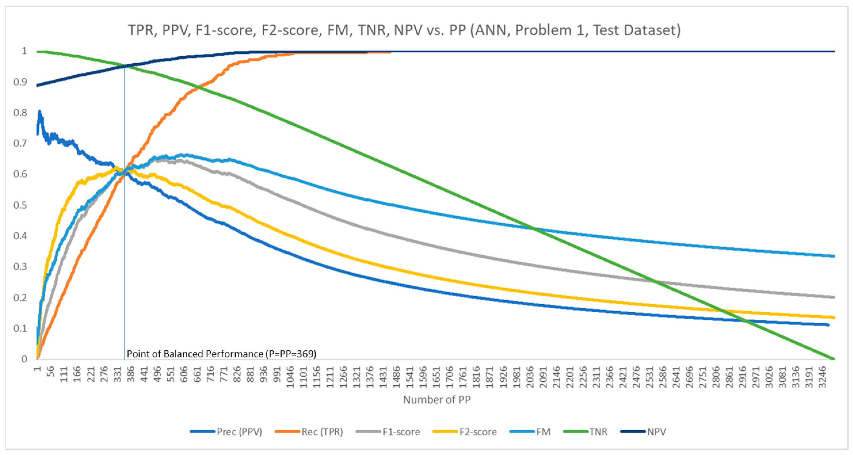
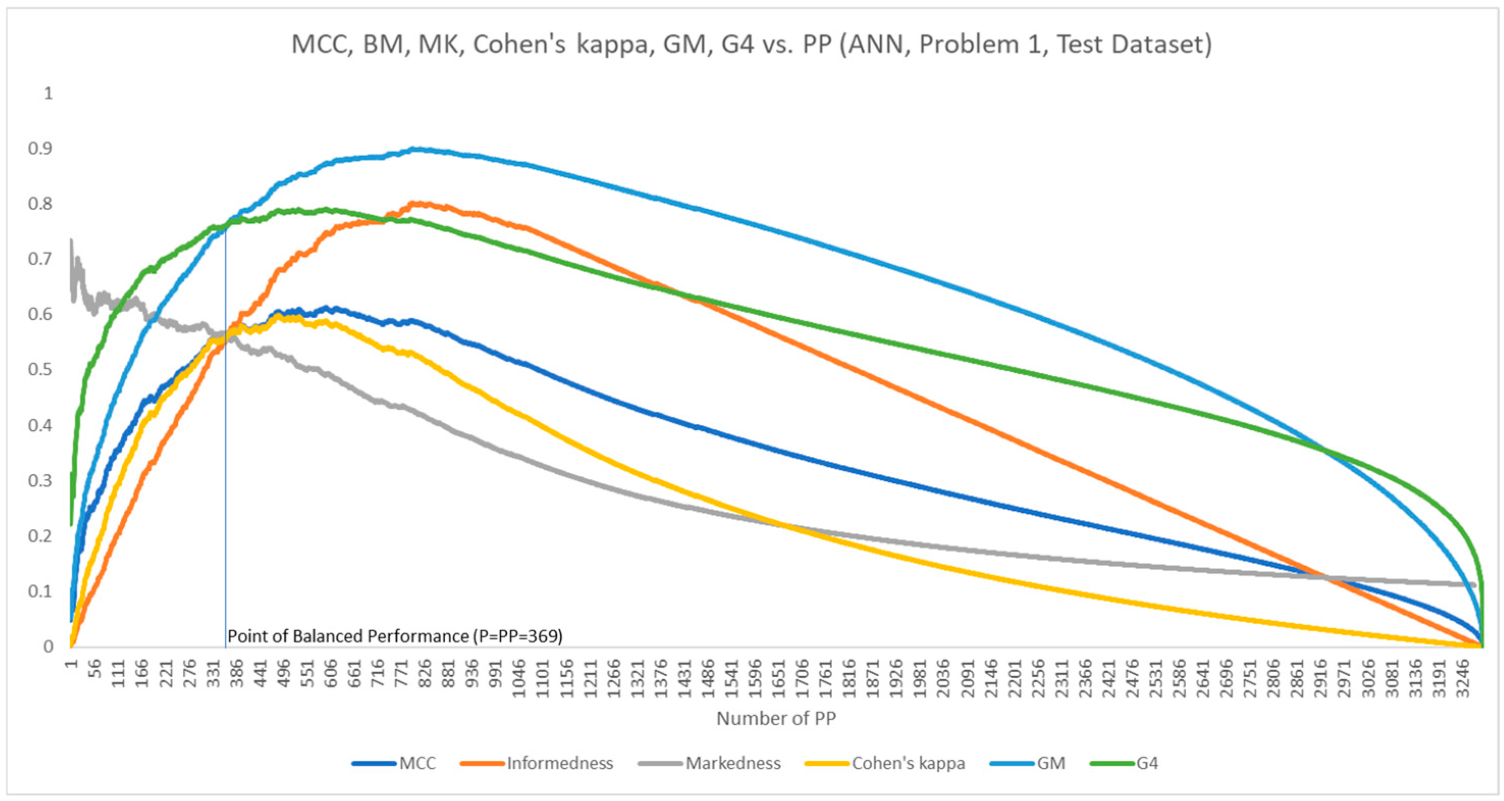
To verify these properties, we consider the application of an ANN to a test dataset of size S = 3295 for Problem 1 (see Appendix A), with P = 369 actual positives. For this example, Figure 1 clearly shows that TPR, PPV, F1-score, F2-score (Fβ-score for β = 2), and FM are equal at the PoBP (i.e., the point at which PP equals P). Moreover, Figure 2 illustrates that MCC, BM, MK, and Cohen’s kappa become equal at the PoBP. Both figures present the metrics vs. the number of PP (ranging from $PP=0$ to $PP=S$) in order to clearly present the conditions that apply at the PoBP (i.e., $PP=P$). This is an equivalent way of presenting the metrics vs. the classification threshold $\theta$ varying from 1 to 0 (since for $\theta =1$, $PP=0$ and for $\theta =0$, $PP=S$).

Figure 2 illustrates that MCC, BM, MK, GM, and G4 are equal at a second point, corresponding to the case where PP equals the number of actual negatives (i.e., $PP=N=2926$ in the example dataset). Unlike PoBP, this point has no specific interest from the classifier performance viewpoint.

Both figures indicate that none of the presented metrics is maximized at the PoBP. However, PoBP provides a tradeoff between pairs of metrics with opposite trends as follows: (a) TPR vs. PPV, (b) TNR vs. NPV, and (c) MCC or BM (Informedness) vs. MK (Markedness).

5.3. Performance Metrics That Become Equivalent at the Point-of-Balanced Performance

In this section, in addition to the metrics that are equal at the PoBP (Table 5), we further show that all binary classification performance metrics are equivalent. This unique property of the PoBP makes it an interesting method for comparing the performance of different classifiers. Let us prove the following theorem for any pair of performance metrics:

Theorem 1. 

If two performance metrics $P{M}_1$, $P{M}_2$ indicate an improved binary classification model performance as the number of True Predictions increases (TP and/or TN) and/or the number of False Predictions decreases (FP and/or FN), then the metrics will be equivalent at the PoBP.

Proof of Theorem 1. 

Let us consider two classifiers, f₁ and f₂, applied to the same dataset for a binary classification problem. As already shown, for each classifier, the PoBP exists and, in general, corresponds to a different PoBP threshold (i.e., ${\theta }_{b1}$ for f₁ and ${\theta }_{b2}$ for f₂). Let us also consider a performance metric $P{M}_1$ which is defined based on any set of parameters of the Confusion Matrix. The metric $P{M}_1$ is defined such that it corresponds to an improved model performance as the number of true predictions (i.e., TP and/or TN) increases and/or the number of false predictions (i.e., FP and/or FN) decreases. This property applies to all metrics presented in Table 2 (e.g., TPR increases with the number of TP, indicating better model performance, while FPR decreases as the number of FP decreases, indicating better model performance).

Apart from the Confusion Matrix elements $\left(TP, FP, FN, TN\right)$, the metric $P{M}_1$ (Table 2) may also depend on parameters like $P, N, PP, PN, S$. At the PoBP these parameters become constant for the same input dataset as $PP=P$ and $PN=N$.

Without loss of generality, let us assume that the higher the $P{M}_1$ value, the better the model performance, and at the PoBP, the following inequality holds:

$$P{M}_1\left(f_1,{\theta }_{b1}\right)\ge P{M}_1\left(f_2,{\theta }_{b2}\right)$$

(20)

Under this assumption and based on the definition of $P{M}_1$, at least one of the parameters, TP, FP, FN, and TN, will be better for the model $f_1$ than the corresponding ones for the model $f_2$ at the PoBP. The term “better” in this case means a higher number of true predictions (for TP, TN) and a lower number of false predictions (for FP, FN).

Without loss of generality, let us assume that Equation (20) applies due to the following property: $TP\left(f_1,{\theta }_{b1}\right)\ge TP\left(f_2,{\theta }_{b2}\right)$. It is easy to show, based on $TP+FP=PP$, $TN+FN=PN$ as well as Equations (4)–(6), that in this case, the following properties apply at the PoBP:

$$\begin{gathered} TP\left(f_1,{\theta }_{b1}\right)\ge TP\left(f_2,{\theta }_{b2}\right)\iff FP\left(f_1,{\theta }_{b1}\right)\le FP\left(f_2,{\theta }_{b2}\right)\iff \\ \iff FN\left(f_1,{\theta }_{b1}\right)\le FN\left(f_2,{\theta }_{b2}\right)\iff TN\left(f_1,{\theta }_{b1}\right)\ge TN\left(f_2,{\theta }_{b2}\right) \end{gathered}$$

(21)

According to these properties, if classifier f₁ has a better performance than classifier f₂ when compared at their PoBP based on any of the parameters: TP, FP, FN, or TN, then f₁ will have a better performance than f₂ for the rest of the parameters. Therefore, if Equation (20) holds, then the properties of Equation (21) will also hold at the PoBP.

Now, let us consider another metric $P{M}_2$ which, as with $P{M}_1$, is defined in such a way that it corresponds to a better model performance as the number of true predictions (i.e., TP and/or TN) increases and/or the number of false predictions (i.e., FP and/or FN) decreases. At the PoBP, assuming that Equation (20) and thus Equation (21) apply, it is evident that $P{M}_2$ will also indicate a better performance for the model $f_1$.

In case that the higher the $P{M}_2$ value, the better the model performance, the previous analysis leads to the following condition at the PoBP:

$$P{M}_2\left(f_1,{\theta }_{b1}\right)\ge P{M}_2\left(f_2,{\theta }_{b2}\right)$$

(22)

Therefore, $P{M}_1$ and $P{M}_2$ will be equivalent (see Equation (2)). Note that if the lower $P{M}_2$ the value, the better the model performance, then $P{M}_1$ and $P{M}_2$ would be again equivalent based on the property of Equation (3).

The above analysis indicates that at the PoBP, any pair of performance metrics that correspond to improved model performance as the number of true predictions (TP and/or TN) increases and/or the number of false predictions (FP and/or FN) decreases will be equivalent. □

Based on the above theorem, all State-of-the-Art performance metrics presented in Table 2 are expected to be either equal or equivalent at the PoBP. The analysis provided in Appendix D on the equivalence of parameters at the PoBP provides the necessary evidence for this property. Therefore, if the performance of two binary classifiers is compared at their PoBP, the comparison conclusion will be the same for any metric of Table 2. In this context, at the PoBP, we need to consider only one metric from Table 2 to compare the performance of two classifiers. Therefore, the problem identified in Table 3 is eliminated, as any pair of metrics at the PoBP yields the same conclusions when comparing the performance of binary classifiers.

Table 6. Performance Metric comparison at the PoBP (Problem 1). The best-performing classifier is marked in bold.

	ANN	LogReg	RF	DT	NB	CNN	XGB
Accuracy	0.9135	0.8932	0.8829	0.9035	0.8914	0.9108	0.9144
Fraction of Inefficiency	0.0865	0.11	0.12	0.10	0.11	0.089	0.0856
True Positive Rate	0.61	0.55	0.47	0.59	0.51	0.60	0.63
True Negative Rate	0.9515	0.94	0.93	0.95	0.94	0.950	0.9517
Balanced Accuracy	0.78	0.75	0.70	0.77	0.73	0.78	0.79
False Positive Rate	0.049	0.06	0.07	0.055	0.06	0.050	0.048
False Negative Rate	0.39	0.45	0.53	0.41	0.49	0.40	0.37
Positive Predictive Value	0.61	0.55	0.47	0.59	0.51	0.60	0.63
Negative Predictive Value	0.951	0.94	0.93	0.945	0.94	0.950	0.952
False Discovery Rate	0.39	0.45	0.53	0.41	0.49	0.40	0.37
False Omission Rate	0.049	0.061	0.066	0.055	0.061	0.050	0.048
F1-Score	0.61	0.55	0.47	0.59	0.51	0.60	0.63
Fβ-Score (β = 2)	0.61	0.55	0.47	0.59	0.51	0.60	0.63
Cohen’s kappa	0.56	0.49	0.40	0.53	0.45	0.55	0.58
Informedness	0.56	0.49	0.40	0.53	0.45	0.55	0.58
Markedness	0.57	0.49	0.40	0.53	0.45	0.55	0.58
Matthews Correlation Coefficient	0.56	0.49	0.40	0.53	0.45	0.55	0.58
Fowlkes–Mallows Index	0.61	0.55	0.47	0.59	0.51	0.60	0.63
Jaccard Index	0.44	0.38	0.30	0.41	0.35	0.43	0.46
Prevalence Threshold	0.220	0.249	0.273	0.234	0.256	0.224	0.217
P4 metric	0.186	0.174	0.156	0.181	0.166	0.185	0.189
Positive Likelihood Ratio	12.62	9.14	7.10	10.73	8.42	12.03	12.98
Negative Likelihood Ratio	0.41	0.47	0.57	0.44	0.52	0.42	0.39
Diagnostics Odd Ratio	31.00	19.27	12.44	24.50	16.30	28.86	33.10
Efficiency Index	10.56	8.36	7.54	9.36	8.21	10.21	10.69
Inefficiency Index	0.095	0.120	0.133	0.107	0.122	0.098	0.094
G-Mean Score	0.76	0.72	0.66	0.74	0.70	0.76	0.77
G4 Score	0.76	0.72	0.66	0.74	0.70	0.76	0.77

provides an overview of the resulting metrics at the PoBP for Problem 1, using the same dataset as in Table 3. Table 6 confirms the theoretical predictions regarding the metrics that become equal at the PoBP. Table 6 also confirms that all metrics are equivalent at the PoBP; as in the example presented, XGB becomes the best-performing classifier at the PoBP for all metrics.

It should be noted that Table 3 and Table 6 indicate that ANN performs similarly to XGB across all metrics. As the scope of the paper is to validate the properties of PoBP rather than identify the best-performing classifier for the specific problem, no further hyperparameter optimization has been performed for ANN and XGB.

6. PoBP at the Receiver Operating Characteristic Curve

In this section, we consider the PoBP in relation to the ROC curve [30]. The ROC curve is a method for analyzing the performance of binary classifiers. ROC is the curve in a two-dimensional space representing the True Positive Rate vs. False Positive Rate as the classification threshold $\theta$ ranges from 0 to 1. Beyond the ROC curve, the Area Under the Curve (AUC) is a metric used to compare different models, taking into account the entire range of classification thresholds [31].

Since the definition of the PoBP of a classification model $f$ is based on a certain classification threshold ${\theta }_b$, it is evident that PoBP corresponds to a single point on the ROC curve corresponding to the pair of coordinates $\left(TPR\left(f,{\theta }_b\right), FPR\left(f,{\theta }_b\right)\right)$.

Comparing two classifiers at their PoBP and taking into account the equivalence of all metrics at the PoBP (and hence the equivalence between TPR and FPR), it is expected that the better a classifier’s performance, the higher its TPR and the lower its FPR at the PoBP. Therefore, the PoBP point on the ROC curve of a more efficient classifier will be located to the left and higher than the PoBP point on the ROC curve of a less efficient classifier.

Moreover, assuming a certain binary classification problem, the following condition applies at the PoBP of a classifier:

$$TPR\left(f,{\theta }_b\right)={\displaystyle \frac{TP\left(f,{\theta }_b\right)}{P}}={\displaystyle \frac{PP\left(f,{\theta }_b\right)-FP\left(f,{\theta }_b\right)}{P}}=1-{\displaystyle \frac{N}{P}}·FPR\left(f,{\theta }_b\right)$$

(23)

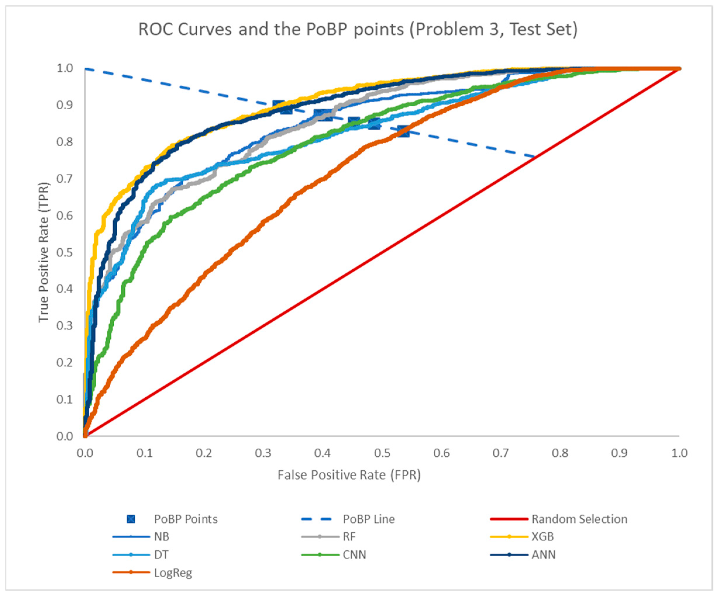
Geometrically, Equation (23) corresponds to a straight line in the ROC space. Therefore, the PoBP point on the ROC curve of any classifier will lie on a line we call the PoBP ROC space line. The endpoints of the PoBP ROC space line can be determined by two points: the ideal classifier with $FPR=0$ and $TPR=1$; the random-guess classifier for which $TPR=FPR$. Equation (23) provides: $TPR\left(f,{\theta }_b\right)=FPR\left(f,{\theta }_b\right)=P/S$ (i.e., the prevalence of the input dataset).

Figure 3 presents the ROC curves for all applied classifiers for a test set of Problem 3 (see Appendix A). The same figure provides the PoBP ROC space line and the PoBP point for each applied classifier, indicating that XGB is the best-performing classifier at the PoBP.

7. Methods for the Identification of the Point-of-Balanced Performance

Following the analysis of the PoBP properties, we focus in this section on identifying the PoBP. Apparently, the identification of PoBP for a classifier applied to an input dataset X and a set of actual class labels Y requires determining the classification threshold for which the number of predicted positives equals the number of actual positives. During the training phase of a classifier, the available dataset is typically split into a training set and, depending on the applied method, a number of test or validation sets [32]. Since the number of actual positives is known for all of these datasets, it is a straightforward process to identify the PoBP when the trained model is applied to any of them. This section further considers the PoBP identification during inference, where the number of actual positives is unknown.

7.1. Methods for the Identification of the Point-of-Balanced Performance During Inference

During inference, the actual class labels are unknown; hence, the PoBP should be approximated. The following three alternative methods are considered:

Method 1: PoBP identification based on Training Dataset Prevalence. Assuming that the Prevalence in the inference dataset $X_{inf}$ is identical to that of the training dataset $X_{train}$, we can estimate the number of positives for the inference dataset $\widehat{P}\left(X_{inf}\right)$ as follows:

$${\displaystyle \frac{P\left(X_{inf}\right)}{S\left(X_{inf}\right)}}\approx {\displaystyle \frac{P\left(X_{train}\right)}{S\left(X_{train}\right)}}\Rightarrow \widehat{P}\left(X_{inf}\right)\approx {\displaystyle \frac{P\left(X_{train}\right)}{S\left(X_{train}\right)}}·S\left(X_{inf}\right)$$

(24)

Method 2: PoBP identification based on the PoBP Classification threshold of the Training dataset. Assuming that both the training $X_{train}$ and the inference datasets $X_{inf}$ follow the same distribution, we may consider that the PoBP classification threshold applied in the training dataset ${\theta }_b\left(X_{train}\right)$ is identical to the one of the inference dataset ${\theta }_b\left(X_{inf}\right)$. This leads directly to the approximation of the PoBP during inference:

$${\theta }_b\left(X_{inf}\right)\approx {\theta }_b\left(X_{train}\right)$$

(25)

Method 3: PoBP identification based on the Actual Label Probabilistic Confusion Matrix (ALP CM) [33]. The ALP CM approximates the actual CM during inference even though the actual class labels are unknown. A good approximation holds for calibrated class probabilities (based on Platt’s method [34] in this paper) and for a substantial input dataset.

This approximation can be used to identify the PoBP during inference by adjusting the decision threshold to achieve the following condition:

$$PP\left(X_{inf}\right)={\widehat{P}}_{ALP}\left(X_{inf}\right)\approx P\left(X_{inf}\right)$$

(26)

Note that Methods 2 and 3 do not rely on the assumption that the prevalence in the inference dataset is identical to that of the training dataset.

7.2. Evaluation of the PoBP Identification Methods During Inference

To evaluate the PoBP identification methods, we split the available datasets into training and test sets and use the test set to simulate the performance of the proposed methods during inference. We consider two different methods for deriving the test datasets: (a) Unbiased Class Mix method: the test datasets are produced based on random selection of samples from the available dataset in a way that they have the same prevalence as the training dataset and (b) Biased Class Mix method: the unbiased mix test datasets are further processed to produce test datasets of shorter size with a prevalence that deviates from the one of the training dataset.

Table 7. The mean absolute error in the estimation of the actual positives in the test set.

Problem	Classifier	Test Set	Set Size	Method 1	Method 2	Method 3
1	SVM	Unbiased	8238	0%	2.8%	1.5%
		Biased	5945	14.3%	5.6%	6.1%
2	RF	Unbiased	200	0%	2.1%	0.8%
		Biased	172	8.4%	5.8%	6.8%
3	NB	Unbiased	6513	0%	0.4%	0.1%
		Biased	5564	6.3%	3.6%	5.2%
4	XGB	Unbiased	29,092	0%	0.5%	0.3%
		Biased	21,847	6.2%	2.9%	3.5%
5	LogReg	Unbiased	5581	0%	3%	1.6%
		Biased	4383	13.2%	7.3%	7.6%

provides the resulting mean absolute error for estimating the number of positives in the test dataset (based on 400 iterations of generating unbiased and biased class-mix test sets) for all problems and for one different classifier per problem (see Appendix A). It is evident that Method 1 results in a higher mean absolute error when the class mix is biased. Methods 2 and 3 appear to be performing better in the presence of bias. It should be noted that the performance of Method 3 depends on the degree to which calibrated class probabilities are in agreement with actual class frequencies.

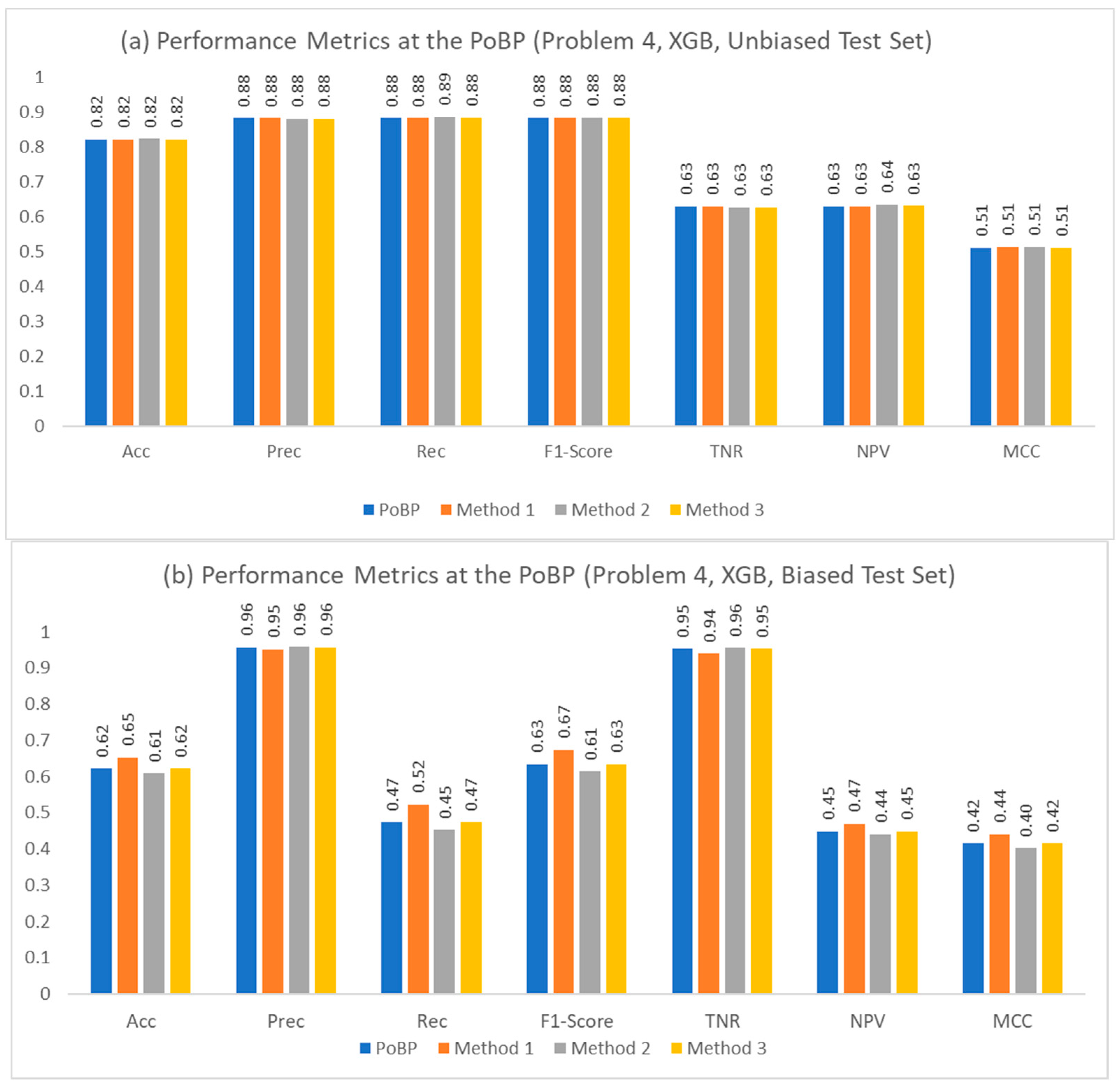
Figure 4 compares a set of performance metrics corresponding to the actual PoBP with those corresponding to the estimated PoBP using each of the above methods. The following indicative set of metrics is considered: Accuracy, Precision, Recall, F1-score, TNR, NPV, and MCC. The figure refers to Problem 4 and the XGB classifier. Figure 4a refers to an unbiased class mix test set of size 29,092 with prevalence 75.8%, and Figure 4b to a biased test set of size 17,096 with prevalence 68.9%. As shown in Table 7, all methods yield accurate PoBP approximations for unbiased input datasets. For that reason, Figure 4a shows that the metrics for the PoBP identified using Methods 1, 2, and 3 are almost identical to those for the actual PoBP. Figure 4b indicates that, for a biased input dataset, the error in identifying the PoBP (see Table 7) is reflected in the deviation between the metrics corresponding to the estimated PoBP and those corresponding to the actual PoBP. Moreover, as expected from Table 7, Figure 4b shows that Methods 2 and 3 perform better than Method 1.

8. Performance at the PoBP vs. Typical Characteristic Points

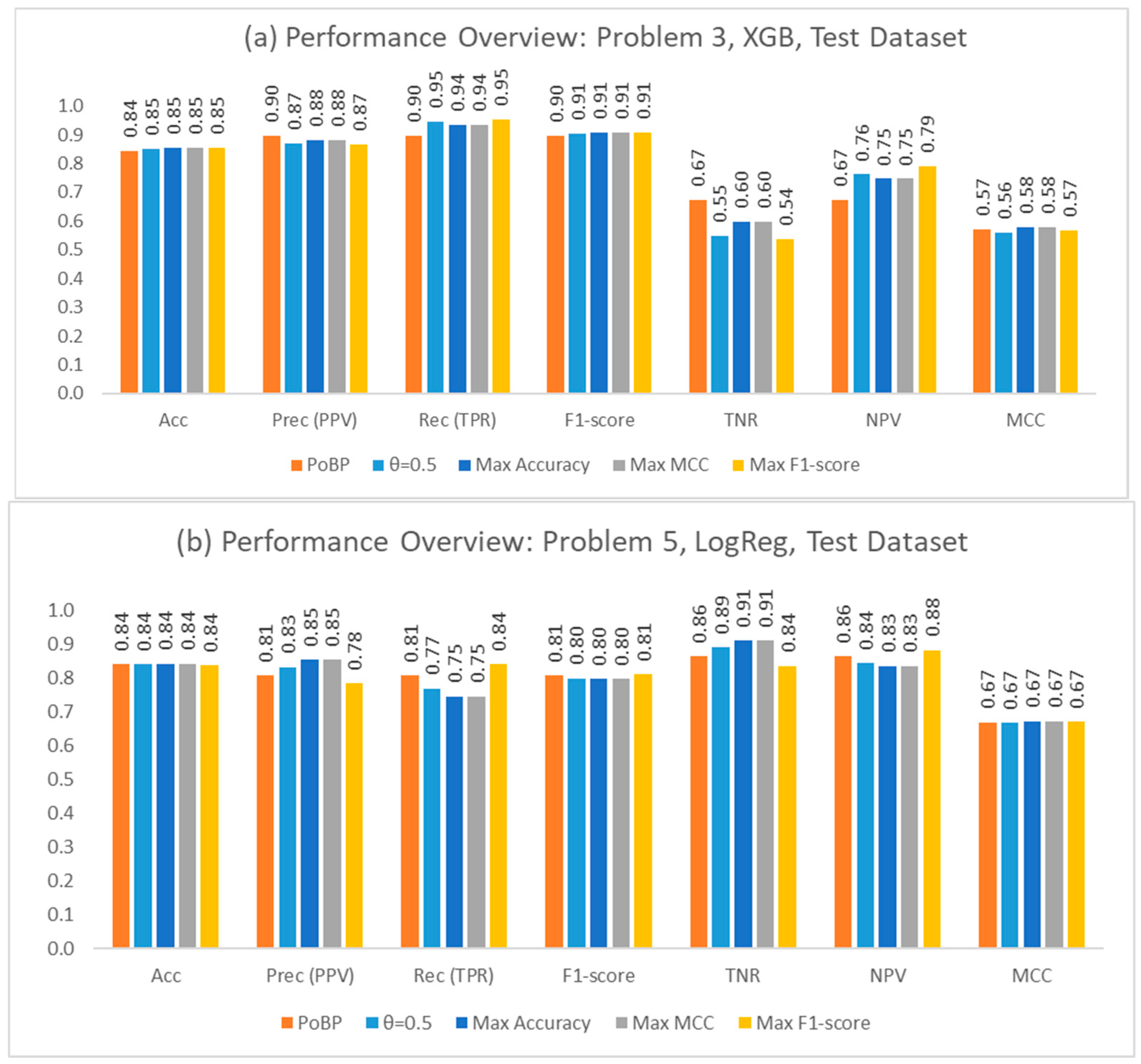
Taking into account that at the PoBP all metrics are equivalent, the selection of the PoBP as the reference point for the analysis of a classification problem appears to be attractive, especially for the identification of the best-performing classifier. On the other hand, as already mentioned, selecting the PoBP does not optimize commonly used performance metrics such as F1-score or MCC. In this section, we compare the performance at the PoBP vs. the following characteristic points typically selected during the study of a classification problem: (a) classification threshold of θ = 0.5, (b) maximum Accuracy, (c) maximum MCC, (d) maximum F1-score.

Figure 5a presents the performance of the PoBP and the above characteristic points for Problem 3 (unbiased test set of size S = 6513, prevalence 76%), XGB classifier, and for a set of metrics: Accuracy, TPR, PPV, F1-Score, TNR, NPV, and MCC. As can be seen, the differences between PoBP and the rest in terms of Accuracy, F1-score, and MMC are quite limited. On the other hand, we observe tradeoffs between TPR and TNR as well as between PPV and NPV. In particular, TPR at the PoBP is 0.90, while at the rest points, it ranges from 0.94 to 0.95. However, TNR is 0.67 at the PoBP, while it ranges from 0.54 to 0.60 at the other performance points. Similarly, the PPV at the PoBP is 0.90 and drops for the rest points, ranging from 0.87 to 0.88, while the NPV at the PoBP is 0.67 and increases for the rest points, ranging from 0.75 to 0.76.

Figure 5b presents the performance of the PoBP and the above characteristic points for Problem 5, LogReg classifier (unbiased test set of size S = 5581, prevalence 41%). Again, the observed difference between PoBP and the rest of the characteristic performance points for Accuracy, F1-score, and MMC is quite limited. Also, we observe tradeoffs between PoBP and the rest points of performance (i.e., TPR vs. TNR, and PPV vs. NPV). However, compared to the example of Figure 5a, in this case, we observe that PoBP has lower TPR and higher TNR than the rest, except at the maximum F1-score, where the opposite applies.

The above presented examples cannot apparently be generalized for all binary classification problems. Instead, they illustrate that the selection of the PoBP can be a viable option for the study of a specific problem. However, methodologically, alternative performance points can be considered, and depending on the importance of certain aspects of the problem (e.g., it may be preferable to have a higher TPR while a lower TNR is not an issue), a different performance point may eventually be selected by a data scientist.

9. Discussion and Conclusions

The paper addresses the binary classification problem and defines the PoBP, the classification threshold for which the number of predicted positives equals the actual number of positive samples, a property of the ideal classifier. It has been proven that at the PoBP, all binary classification performance metrics are equivalent, i.e., they yield the same results when comparing the performance of different binary classifiers. This is a significant advantage for analyzing real-world problems, as the wide variety of binary classification performance metrics in the literature often yields different conclusions about the best-performing classifier.

The literature [7,8,9,10,11,12,13,14,15,16,17,18,19,20,21,22,23,24,25,26,27,28,29] has thus far focused on the advantages and disadvantages of certain performance metrics, proposed new metrics, or considered methods to assess the efficiency of different metrics. From this viewpoint, the current paper takes a different direction by introducing simple concepts, such as equivalent performance metrics and the definition of the PoBP. The paper shows that the observed differences in the performance of the metrics are eliminated at the PoBP. This property allows for comparing different classifiers at their PoBP using a single metric, thereby simplifying the problem of selecting the most appropriate metric.

Given that the ROC Curve [30] is another common method for analyzing the performance of different classifiers, the paper explores the geometrical representation of the PoBP in the ROC space. The PoBP of a classifier is a single point on the ROC curve, while it is proven that the PoBP of any classifier of the same binary classification problem belongs to a straight line called the PoBP ROC curve line. As expected, the better classifier has better performance across both metrics of the ROC space.

The identification of the PoBP during the training phase is trivial, whereas an approximation method is required during inference, since the number of actual positives is unknown in that case. The paper provides three alternative methods using: (a) the prevalence in the training set, (b) the PoBP classification threshold during the training phase, and (c) the ALP Confusion Matrix. Based on the analysis of real-world binary classification problems, it is shown that the last two methods provide a good approximation of the PoBP performance, even when the prevalence in the inference set differs from that in the training dataset.

The paper then considers whether PoBP should be the preferred point of performance for analyzing a binary classification problem. To address this issue, we present examples of a classifier’s performance at the PoBP vs. other commonly used points of performance (i.e., classification threshold of 0.5, maximum Accuracy, maximum MCC, and maximum F1-score). The example results indicate that PoBP may perform similarly across certain metrics (Accuracy, MCC, and F1-score), while tradeoffs may occur in other metrics (TPR, TNR, PPV, and NPV). Although these results cannot be considered applicable to all binary classification problems, the paper provides a method for comparing PoBP with other performance metrics. Depending on the specific problem requirements, the data scientist may select either the PoBP or an alternative point that best fits the problem’s needs.

The next research steps include various topics such as: (a) the analysis of a multi-class classification problem aiming at the generalization of the PoBP concept, (b) the definition of equivalent performance metrics will be exploited to investigate different characteristic points of performance, and (c) the investigation of the applicability of the PoBP concept for classifiers with non-probabilistic output (e.g., k-NN).

In conclusion, the paper, through the introduction of the PoBP concept, provides new insights and a relevant methodology that simplifies the performance analysis of binary classification.

References

1. Alpaydin, E. Introduction to Machine Learning; The MIT Press: Cambridge, MA, USA, 2010; ISBN 978-0-262-01243-0. [Google Scholar]
2. Sarker, I.H. Machine Learning: Algorithms, Real-World Applications and Research Directions. SN Comput. Sci. 2021, 2, 160. [Google Scholar] [CrossRef] [Scilit]
3. Garg, A.; Roth, D. Understanding probabilistic classifiers. In Proceedings of the ECML 2001 12th European Conference on Machine Learning, LNAI 2167, Freiburg, Germany, 5–7 September 2001; pp. 179–191. [Google Scholar]
4. Stehman, S.V. Selecting and interpreting measures of thematic classification accuracy. Remote Sens. Environ. 1997, 62, 77–89. [Google Scholar] [CrossRef] [Scilit]
5. Ting, K.M. Confusion Matrix. In Encyclopedia of Machine Learning and Data Mining; Springer: Berlin/Heidelberg, Germany, 2010. [Google Scholar]
6. Uddin, S.; Khan, A.; Hossain, M.; Moni, M.A. Comparing different supervised machine learning algorithms for disease prediction. BMC Med. Inform. Decis. Mak. 2019, 19, 281. [Google Scholar] [CrossRef] [Scilit]
7. Chicco, D.; Jurman, G. The advantages of the Matthews correlation coefficient (MCC) over F1 score and accuracy in binary classification evaluation. BMC Genom. 2020, 21, 6. [Google Scholar] [CrossRef] [Scilit]
8. Cao, C.; Chicco, D.; Hoffman, M.M. The MCC-F1 curve: A performance evaluation technique for binary classification. arXiv 2020, arXiv:2006.11278. [Google Scholar] [CrossRef] [Scilit]
9. Chicco, D.; Jurman, G. The Matthews correlation coefficient (MCC) should replace the ROC AUC as the standard metric for assessing binary classification. BioData Min. 2023, 16, 4. [Google Scholar] [CrossRef] [Scilit] [PubMed] [PubMed Central]
10. Chicco, D.; Warrens, M.; Jurman, G. The Matthews Correlation Coefficient (MCC) is More Informative Than Cohen’s Kappa and Brier Score in Binary Classification Assessment. IEEE Access 2021, 9, 78368–78381. [Google Scholar] [CrossRef] [Scilit]
11. Chicco, D.; Jurman, G. A statistical comparison between Matthews correlation coefficient (MCC), prevalence threshold, and Fowlkes–Mallows index. J. Biomed. Inform. 2023, 144, 104426. [Google Scholar] [CrossRef] [Scilit]
12. Itaya, Y.; Tamura, J.; Hayashi, K.; Yamamoto, K. Asymptotic Properties of Matthews Correlation Coefficient. Stat. Med. 2025, 44, e10303. [Google Scholar] [CrossRef] [Scilit]
13. Zhu, Q. On the performance of Matthews correlation coefficient (MCC) for imbalanced dataset. Pattern Recognit. Lett. 2020, 136, 71–80. [Google Scholar] [CrossRef] [Scilit]
14. Shao, G.; Tang, L.; Liao, J. Overselling overall map accuracy misinforms about research reliability. Landsc. Ecol. 2019, 34, 2487–2492. [Google Scholar] [CrossRef] [Scilit]
15. Leeflang, M.M.; Bossuyt, P.M.; Irwig, L. Diagnostic test accuracy may vary with prevalence: Implications for evidence-based diagnosis. J. Clin. Epidemiol. 2009, 62, 5–12. [Google Scholar] [CrossRef] [Scilit]
16. Powers, D. The problem with kappa. In Proceedings of the 13th Conference of the European Chapter of the Association for Computational Linguistics (EACL ‘12); Association for Computational Linguistics: Avignon, France, 2012; pp. 345–355. [Google Scholar]
17. Powers, D.M.W. Evaluation: From Precision, Recall and F-Measure to ROC, Informedness, Markedness & Correlation. arXiv 2011, arXiv:2010.16061. [Google Scholar]
18. Larner, A.J. Efficiency Index for Binary Classifiers: Concept, Extension, and Application. Mathematics 2023, 11, 2435. [Google Scholar] [CrossRef] [Scilit]
19. Kuncheva, L.I.; Arnaiz-González, Á.; Díez-Pastor, J.-F.; Gunn, I.A.D. Instance selection improves geometric mean accuracy: A study on imbalanced data classification. Prog. Artif. Intell. 2019, 8, 215–228. [Google Scholar] [CrossRef] [Scilit]
20. Marra, A. G4 & the balanced metric family—A novel approach to solving binary classification problems in medical device validation & verification studies. BioData Min. 2024, 17, 43. [Google Scholar] [CrossRef] [Scilit]
21. Lipton, Z.C.; Elkan, C.; Naryanaswamy, B. Optimal Thresholding of Classifiers to Maximize F1 Measure. In Proceedings of the Machine Learning and Knowledge Discovery in Databases: European Conference, ECML PKDD; Springer: Berlin/Heidelberg, Germany, 2014; Volume 8725, pp. 225–239. [Google Scholar]
22. Canbek, G.; Sagiroglu, S.; Temizel, T.T.; Baykal, N. Binary classification performance measures/metrics: A comprehensive visualized roadmap to gain new insights. In 2017 International Conference on Computer Science and Engineering (UBMK); IEEE: New York, NY, USA, 2017; pp. 821–826. [Google Scholar] [CrossRef] [Scilit]
23. Hernández-Orallo, J.; Flach, P.; Ferri, C. A unified view of performance metrics: Translating threshold choice into expected classification loss. J. Mach. Learn. Res. 2012, 13, 2813–2869. [Google Scholar]
24. Christen, P.; Hand, D.J.; Kirielle, N. A Review of the F-Measure: Its History, Properties, Criticism, and Alternatives. ACM Comput. Surv. 2023, 56, 73. [Google Scholar] [CrossRef] [Scilit]
25. Hand, D.J.; Christen, P.; Kirielle, N. F*: An interpretable transformation of the F-measure. Mach Learn. 2021, 110, 451–456. [Google Scholar] [CrossRef] [Scilit] [PubMed] [PubMed Central]
26. Kim, H.; Park, Y. Calibrating F1 Scores for Fair Performance Comparison of Binary Classification Models with Application to Student Dropout Prediction. IEEE Access 2025, 13, 136554–136567. [Google Scholar] [CrossRef] [Scilit]
27. Walauskis, M.A.; Khoshgoftaar, T.M. Choosing the Right Metrics: A Study of Performance Measurement for Binary Classification in Imbalanced and Big Data. Int. FLAIRS Conf. Proc. 2025, 38. [Google Scholar] [CrossRef] [Scilit]
28. Canbek, G.; Taskaya Temizel, T.; Sagiroglu, S. BenchMetrics: A systematic benchmarking method for binary classification performance metrics. Neural Comput. Applic 2021, 33, 14623–14650. [Google Scholar] [CrossRef] [Scilit]
29. Shirdel, M.; Di Mauro, M.; Liotta, A. Worthiness Benchmark: A novel concept for analyzing binary classification evaluation metrics. Inf. Sci. 2024, 678, 120882. [Google Scholar] [CrossRef] [Scilit]
30. Fawcett, T. An introduction to ROC analysis. Pattern Recognit. Lett. 2006, 27, 861–874. [Google Scholar] [CrossRef] [Scilit]
31. Hanley, J.A.; McNeil, B.J. The meaning and use of the area under a receiver operating characteristic (ROC) curve. Radiology 1982, 143, 29–36. [Google Scholar] [CrossRef] [Scilit] [PubMed]
32. Refaeilzadeh, P.; Tang, L.; Liu, H. Cross-Validation. In Encyclopedia of Database Systems; Liu, L., Özsu, M.T., Eds.; Springer: Boston, MA, USA, 2009. [Google Scholar] [CrossRef] [Scilit]
33. Markoulidakis, I.; Markoulidakis, G. Probabilistic Confusion Matrix: A Novel Method for Machine Learning Algorithm Generalized Performance Analysis. Technologies 2024, 12, 113. [Google Scholar] [CrossRef] [Scilit]
34. Niculescu-Mizil, A.; Caruana, R. Predicting good probabilities with supervised learning. In Proceedings of the 22nd International Conference on Machine Learning (ICML’ 05), Bonn, Germany, 7–11 August 2005; Association for Computing Machinery: New York, NY, USA, 2005; pp. 625–632. [Google Scholar]
35. Moro, S.; Cortez, P.; Rita, P. A data-driven approach to predict the success of bank telemarketing. Decis. Support Syst. 2014, 62, 22–31. [Google Scholar] [CrossRef] [Scilit]
36. Hofmann, H. Statlog (German Credit Data). Machine Learning Repository. 1994, Volume 53. Available online: https://archive.ics.uci.edu/dataset/144/statlog+german+credit+data (accessed on 20 February 2026).
37. Becker, B.; Kohavi, R. Adult [Dataset]. UCI Machine Learning Repository. 1996. Available online: https://archive.ics.uci.edu/dataset/2/adult (accessed on 20 February 2026).
38. Australia Meteorology Government Bureau. Available online: http://www.bom.gov.au/ (accessed on 20 February 2026).
39. Garcia-Ceja, E.; Riegler, M.; Jakobsen, P.; Tørresen, J.; Nordgreen, T.; Oedegaard, K.J.; Fasmer, O.B. A Motor Activity Database of Depression Episodes in Unipolar and Bipolar Patients. In Proceedings of the MMSys’18 9th ACM on Multimedia Systems Conference, Amsterdam, The Netherlands, 12–15 June 2018; Available online: https://dl.acm.org/doi/pdf/10.1145/3204949.3208125 (accessed on 20 February 2026).
40. Quinlan, J.R. Induction of decision trees. Mach. Learn. 1986, 1, 81–106. [Google Scholar] [CrossRef] [Scilit]
41. Rokach, L.; Maimon, O.Z. Data Mining with Decision Trees: Theory and Applications; World Scientific: Singapore, 2008; Volume 69. [Google Scholar]
42. Basak, D.; Srimanta, P.; Patranabis, D.C. Support Vector Regression. Neural Inf. Process.-Lett. Rev. 2007, 11, 203–224. [Google Scholar]
43. Abe, S. Support Vector Machines for Pattern Classification, 2nd ed.; Advances in Computer Vision and Pattern Recognition; Springer: London, UK, 2010. [Google Scholar] [CrossRef] [Scilit]
44. Cortes, C.; Vapnik, V. Support-vector networks. Mach. Learn. 1995, 20, 273–297. [Google Scholar] [CrossRef] [Scilit]
45. Pal, M. Random forest classifier for remote sensing classification. Int. J. Remote Sens. 2005, 26, 217–222. [Google Scholar] [CrossRef] [Scilit]
46. Breiman, L. Random forests. Mach. Learn. 2001, 45, 5–32. [Google Scholar] [CrossRef] [Scilit]
47. Walczak, S.; Cerpa, N. Artificial Neural Networks, Encyclopedia of Physical Science and Technology, 3rd ed.; Academic Press: Cambridge, MA, USA, 2003; pp. 631–645. ISBN 9780122274107. [Google Scholar] [CrossRef] [Scilit]
48. Doulamis, A.; Doulamis, N.; Kollias, S. On-line retrainable neural networks: Improving the performance of neural networks in image analysis problems. IEEE Trans. Neural Netw. 2000, 11, 137–155. [Google Scholar] [CrossRef] [PubMed]
49. Haykin, S. Neural Networks: A Comprehensive Foundation; Prentice-Hall Inc.: Upper Anhe, NJ, USA, 2007. [Google Scholar]
50. Doulamis, A.; Doulamis, N.; Protopapadakis, E.; Voulodimos, A. Combined Convolutional Neural Networks and Fuzzy Spectral Clustering for Real Time Crack Detection in Tunnels. In Proceedings of the 2018 25th IEEE International Conference on Image Processing (ICIP), Athens, Greece, 7–10 October 2018; pp. 4153–4157. [Google Scholar] [CrossRef] [Scilit]
51. Albawi, S.; Mohammed, T.A.; Al-Zawi, S. Understanding of a convolutional neural network. In Proceedings of the 2017 International Conference on Engineering and Technology (ICET), Antalya, Turkey, 21–23 August 2017; pp. 1–6. [Google Scholar] [CrossRef] [Scilit]
52. Chauhan, R.; Ghanshala, K.K.; Joshi, R.C. Convolutional Neural Network (CNN) for Image Detection and Recognition. In Proceedings of the 2018 1st International Conference on Secure Cyber Computing and Communication (ICSCCC), Jalandhar, India, 15–17 December 2018; pp. 278–282. [Google Scholar] [CrossRef] [Scilit]
53. Haouari, B.; Amor, N.B.; Elouedi, Z.; Mellouli, K. Naïve possibilistic network classifiers. Fuzzy Sets Syst. 2009, 160, 3224–3238. [Google Scholar] [CrossRef] [Scilit]
54. Hosmer, D.W., Jr.; Lemeshow, S.; Sturdivant, R.X. Applied Logistic Regression; JohnWiley & Sons: Hoboken, NJ, USA, 2013; Volume 398. [Google Scholar]
55. Chen, T.; Guestrin, C. Xgboost: A scalable tree boosting system. In Proceedings of the 22nd ACM Sigkdd International Conference on Knowledge Discovery and Data Mining, San Francisco, CA, USA, 13–17 August 2016; pp. 785–794. [Google Scholar]
Figure 1. Metric equalities at the PoBP (P = PP = 369): TPR, PPV, F1-score, F2-score, FM, TNR, NPV vs. the number of PP for the ANN classifier, Problem 1, Test dataset (S = 3295).
Technologies 14 00139 g001
Figure 2. Metric equalities at the PoBP (P = PP = 369): MCC, BM, MK, Cohen’s kappa, GM, G4 vs. the number of PP for ANN Classifier, Problem 1, Test dataset (S = 3295).
Technologies 14 00139 g002
Figure 3. The ROC curves and PoBP points for the classifiers applied to Problem 3 (Test set size 2606).
Technologies 14 00139 g003
Figure 4. Performance metrics for the actual vs. the estimated PoBP: (a) Unbiased, (b) Biased Test set (Problem 4, XGB classifier).
Technologies 14 00139 g004
Figure 5. Selected performance metrics at the PoBP vs. other characteristic points of performance: (a) Problem 3, XGB, test dataset of size S = 6513, (b) Problem 5, LogReg, test dataset of size S = 5581.
Technologies 14 00139 g005