Multi-Scale ConvNeXt for Robust Brain Tumor Segmentation in Multimodal MRI

Abstract

Vision Transformer (ViT) models are well known for effectively capturing global contextual information through self-attention. In contrast, ConvNeXt’s hierarchical convolutional inductive bias enables the extraction of robust multi-scale features at lower computational and memory cost, making it suitable for deployment in systems with limited annotation and constrained resources. Accordingly, a multi-scale UNet architecture based on a ConvNeXt backbone is proposed for brain tumor segmentation; it is equipped with a spatial latent module and Reverse Attention (RA)-guided skip connections. This framework jointly models long-range context and delineates reliable boundaries. Magnetic resonance images drawn from the BraTS 2021, 2023, and 2024 datasets serve as case studies for evaluating brain tumor segmentation performance. The incorporated multi-scale features notably improve the segmentation of small enhancing regions and peripheral tumor boundaries, which are frequently missed by single-scale baselines. On BraTS 2021, the model achieves a Dice similarity coefficient (DSC) of 0.8956 and a mean intersection over union (IoU) of 0.8122, with a sensitivity of 0.8761, a specificity of 0.9964, and an accuracy of 0.9878. On BraTS 2023, it attains a DSC of 0.9235 and an IoU of 0.8592, with a sensitivity of 0.9037, a specificity of 0.9977, and an accuracy of 0.9904. On BraTS 2024, it yields a DSC of 0.9225 and an IoU of 0.8575, with a sensitivity of 0.8989, a specificity of 0.9979, and an accuracy of 0.9903. Overall, the segmentation results provide spatially explicit contours that support lesion-area estimation, precise boundary delineation, and slice-wise longitudinal assessment.

1. Introduction

Brain and central nervous system (CNS) tumors have a significant impact on public health among adults and young adults aged 15–39 years [1] and remain an important cause of mortality worldwide [2]. Brain tumors arise when malignant cells proliferate uncontrollably within the brain tissue. The CNS, including the brain and spinal cord, plays a central role in brain tumor development and abnormal tissue growth. Recent findings in meningeal lymphatic vessels provide new insights into immune responses during tumor progression [3]. As tumors expand, they alter morphology and local biomechanics by generating tensile forces that disrupt mechanical homeostasis, thereby exposing cancer cells to heterogeneous mechanical stimuli [4]. Notably, brain tumors represent up to 90% of all CNS neoplasms, with the remaining cases appearing in the spinal cord or other CNS structures [5].

Interestingly, tumors do not grow regularly or systematically, making it impossible to determine the location, type, or texture of the brain where the cancer develops [6]. Therefore, it is essential to acknowledge that malignant tissues can exhibit disorders similar to those found in healthy brain tissue. Although benign tumors are defined by their slow growth, they can still pose a significant risk if timely treatment is not provided (e.g., neurological damage may occur due to mass effect) [7]. Secondary brain tumors, also known as metastatic lesions, arise when cancer cells spread from primary sites and establish secondary growths within the brain parenchyma [8].

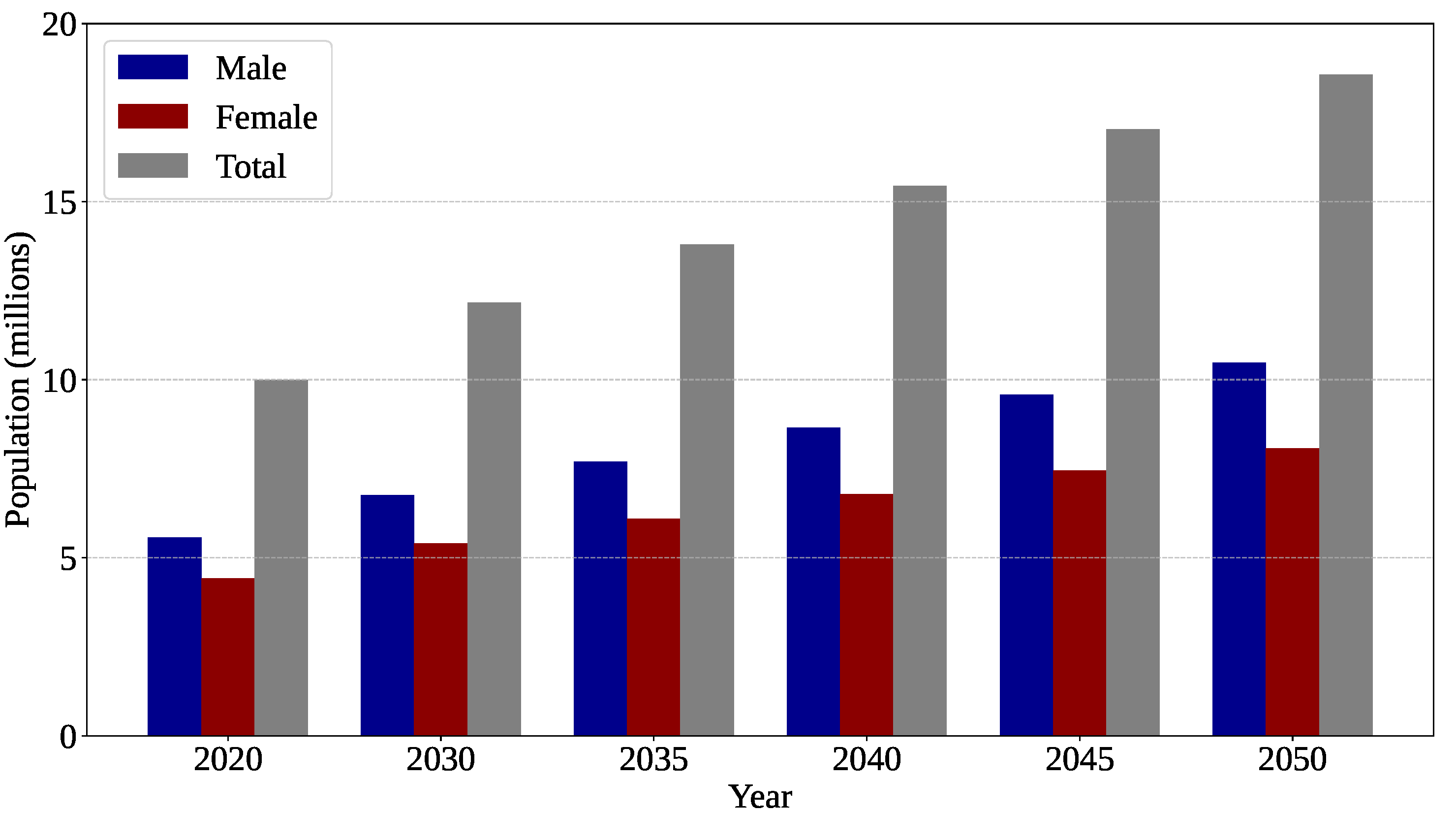
According to the National Cancer Institute (NCI), the United States leads the list in the number of brain tumor deaths. The relative survival from brain tumors over five years, from 2015 to 2021, is approximately 33%, with 24.8 thousand new cases projected for the current year (2025) and a death toll of 18.3 thousand [9,10]. Figure 1 presents a quantitative analysis, estimating the global increase in mortality attributable to brain tumors from 2020 to 2040. Furthermore, Filho et al. [11] report a projected 47% increase in new cases by 2045 compared to 2022, emphasizing the urgency of reducing the new case rate by at least 2% per year to keep the 2045 incidence below 2022 levels.

The primary treatment modalities for brain tumors consist of surgery, radiation therapy, chemotherapy, and immunotherapy [13]. Therefore, early tumor monitoring and detection are fundamental to preserving neurological function.

In clinical practice, the main clinical imaging modalities for visualizing the internal structure of the brain are X-ray, computed tomography (CT), and magnetic resonance imaging (MRI) [13]. However, X-ray and CT studies use ionizing radiation, with CT delivering higher doses [14]. Ionizing radiation can cause long-term health problems, such as increasing the risk of cancer [13].

In contrast, MRI is a non-invasive diagnostic modality that provides high-quality brain and surrounding soft-tissue visualization without radiation [15], generating high-contrast images. Therefore, MRI has become indispensable for neuro-oncological evaluation [16]. Specifically, MRI uses strong magnetic fields to transmit radio-frequency energy signals through tissues (typically ranging from 20 kHz to 300 MHz [17]). As these tissues contain water, the radio-frequency signal transiently misaligns the water protons in the surrounding tissues. As these protons return to their original alignment, they release energy, which is scanned and transformed into an image [18].

MRI encompasses various complementary modalities: T1, T1-C, T2, and FLAIR [19]. Each imaging modality provides a comprehensive understanding of both the structural and functional tumor characteristics. T1-weighted imaging is used to highlight the anatomy and structure of the region under study. A bright appearance indicates the presence of fat, while fluids such as cerebrospinal fluid appear dark [20]. Similarly, T2-weighted images are susceptible to fluids and can detect inflammation, tumors, and lesions, as fluids appear bright in these images. Moreover, T1-weighted contrast (T1-C) uses a contrast agent to enhance tissue visibility, making abnormalities such as tumors and inflammation appear brighter [21]. Lastly, fluid-attenuated inversion recovery (FLAIR) uses T2-weighted images and suppresses cerebrospinal fluid to enhance the contrast between fluids and surrounding tissues, thus facilitating the detection of superficial brain lesions [22].

Figure 2 presents three imaging modalities (a–c) along with the corresponding ground-truth tumor mask (d). The purpose of displaying this tumor image is to illustrate which modality provides the most precise visualization of the tumor, with the T2-weighted MRI modality offering the most reliable depiction of the tumor core (see Figure 2c) while FLAIR provides complementary information on peritumoral edema and diffuse infiltration.

MRI images must be processed and analyzed after acquisition. Thus, digital image processing is essential, with a particular emphasis on image segmentation techniques for tumor identification. In biomedical imaging, segmentation may help identify tumors with precise spatial locations [23]. Therefore, accurate tumor location is crucial for specialists to make an informed decision about the most appropriate course of action and treatment. These actions may involve surgical resection, adjuvant therapy, or a longitudinal follow-up procedure to prevent progression or recurrence.

With the advent of convolutional neural networks (CNNs), deep learning has increasingly gained prominence in medical image analysis [24]. CNNs can automatically extract hierarchical tumor features by using sliding filters during convolution. CNNs have been applied in several fields, ranging from object detection [25] to the automatic segmentation of brain tumors [26]. However, CNNs contain small filters that cannot effectively detect features at different scales. As a result, conventional CNNs may struggle to capture the global context within an image [27]. To overcome these limitations, Vision Transformers (ViTs) introduce self-attention mechanisms by aggregating featured information across the entire spatial domain from the first layer.

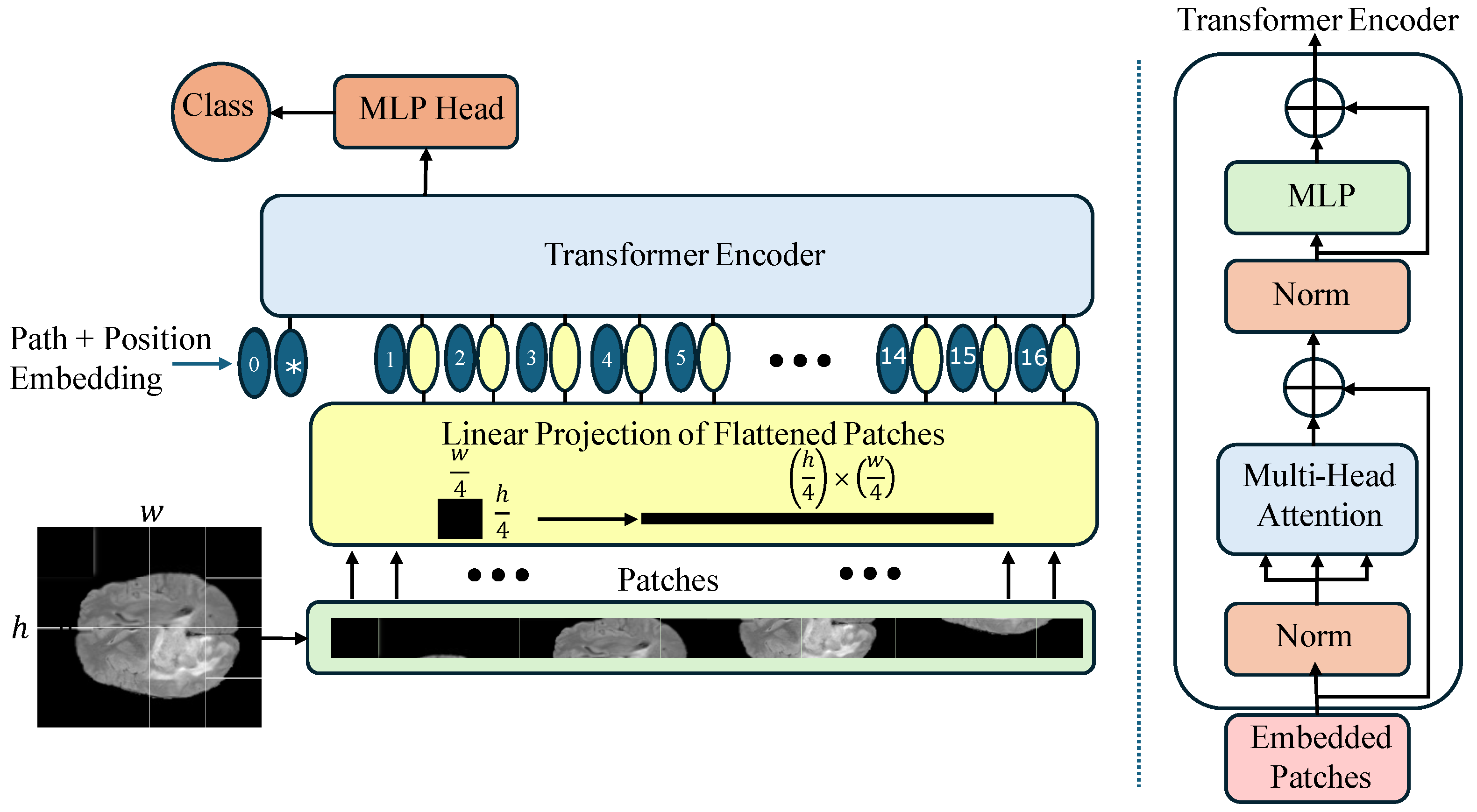
Figure 3 shows the basic architecture of a Vision Transformer (ViT), which includes image splitting into patches, patch tokenization, positional encoding, stacked Transformer encoder blocks, and the MLP-based classification head. Transformer models were originally developed for natural language processing (NLP), where they excel at capturing long-range contextual relationships within text [28]. In computer vision, the ViT follows a similar approach, extracting non-overlapping, fixed-size patches from the input image [29]. Subsequently, each patch is flattened into a vector, forming a sequence of tokens. Finally, the resulting token sequence is processed by stacked self-attention blocks, whose global receptive field enables the model to relate distant regions from the very first layer.

The primary feature of ViT is the self-attention (SA) mechanism, which computes relationships among all patches, independent of spatial location (distance), to obtain a robust global context [27]. This study explores the potential use of ConvNeXt, a Transformer-inspired modern convolutional network, to improve semantic segmentation by combining the inductive biases of CNNs with the scalability characteristics of Transformer architectures. The main contributions of this paper are summarized below:

• Integrating a customized ConvNeXt backbone, fine-tuned for MRI inputs to exploit its hierarchical convolutional blocks, enables the extraction of rich multi-scale features for more precise delineation of heterogeneous tumor structures.
• Implementing an automatic slice selection module that supplies a ConvNeXt-based model with the BraTS 2021 [30], 2023 [31], and 2024 [32] slices exhibiting the highest tumor burden, thereby improving segmentation accuracy while reducing redundancy across slices.
• Incorporating a UNet decoder enhanced with Reverse Attention (RA) modules applied to the skip connections. This design enables the model to suppress background regions and emphasize salient tumor structures, thereby improving the delineation of complex and heterogeneous tumor boundaries.

2. Literature Review

While UNet architectures based on CNNs have achieved state-of-the-art image segmentation performance by learning rich hierarchical representations, CNNs remain inherently limited in modeling long-range dependencies and non-local object correlations within an image [33]. In contrast, ViT models employ self-attention mechanisms that explicitly encode global context, enabling them to capture extended pixel-level relationships with greater efficacy [28].

Andrade-Miranda et al. [33] compared several Transformer models, specifically a hybrid pipeline, in a controlled brain tumor segmentation experiment on the BraTS 2021 dataset. The model adopts the familiar U-shaped encoder–decoder design, where the encoder uses a pre-trained Residual Network (ResNet) backbone on ImageNet to capture compact features at multiple scales. In deep learning, a backbone is a pre-trained feature extractor whose reused weights accelerate convergence and improve generalization [34].

Yang et al. [35] proposed a Convolution-and-Transformer network (COTRNet) that transfers the learning capabilities of an ImageNet-trained classifier and introduces a novel method called deep supervision. The efficacy of deep supervision in improving training stems from its ability to provide supplementary loss functions at intermediate layers.

Chen and Yang [36] employed a combination of a UNet architecture and a Swin Transformer network, naming it CBAM-TransUNet; it incorporates a 3D multimodal image attention mechanism into the structure for tumor edge detection and segmentation. Likewise, using 2D images, Jia and Shu [37] employed a UNet architecture with a CNN transformer, called BiTr-Unet. Extending this approach to 3D volumes, Jiang et al. [38] employed SwinBTS, a UNet network that replaces the convolutional layers with 3D Swin Transformer blocks in the encoder and decoder. The Swin Transformer reduces the number of parameters and improves feature learning. In this way, the BraTS 2021 dataset is processed in its complete 3D format.

Recently, ZongRen et al. [39] introduced DenseTrans, a lightweight UNet++ variant that integrates Swin Transformer blocks to enrich local convolutional features with global contextual information on the BraTS 2021 dataset. Convolutional layers capture fine-grained details, while shift-window self-attention models long-range dependencies in the high-resolution paths. Additionally, Praveen et al. [40] proposed a hybrid architecture combining the Swin Transformer, ResNet, and UNet for meningioma segmentation on the BraTS 2023 dataset. In this framework, the Swin Transformer enriches multi-scale feature representation, the ResNet branch contributes residual connections that stabilize the training of deeper layers, and the UNet decoder preserves fine-grained spatial information for precise tumor delineation.

Similarly, Lin et al. [41] proposed a hybrid model combining UNet and Transformer on the BraTS 2021 dataset. They worked with volumetric images, using two modalities in parallel as input to a dual-branch hybrid encoder block, assigning different weights to each modality. The essential characteristics extracted from these volumes are passed to a parallel block, the Modality-Correlated Cross-Attention (MCCA), which extracts both local and long-range information.

Dobko et al. [42] modified the TransBTS model to improve segmentation performance by incorporating Squeeze-and-Excitation blocks. They also replaced the positional encoding in the Transformer with trainable Multi-Layer Perceptron (MLP) embeddings, enabling the model to adjust input sizes during inference. Finally, they integrated a modified architecture into the nnUNet to further improve performance.

Bhagyalaxmi and Dwarakanath [43] proposed a multistage framework that combines classical filtering, Transformer-based encoding, and chaos-inspired optimization for segmenting brain tumors in MRI. In the first stage, images from BraTS 2020–2023 are denoised using a Probabilistic Hybrid Wiener Filter (PHWF) and then encoded by a lightweight 3D Convolutional Vision Transformer (3D-ViT). The resulting tokens drive a Dilated Channel-Gate UNet, whose training is steered by the Chaotic Harris Shrinking Spiral Optimization Algorithm (CHSOA). This PHWF + 3D-ViT + CDCG-UNet pipeline consistently improves delineation of the whole tumor, the tumor core, and the enhanced tumor regions across all evaluated datasets.

Wu and Li [44] used a ConvNeXt module within a UNet network, an integral component of the decoder section, serving as a feature extractor for segmenting urban scenes. Deploying a depth-based character extraction network as the encoder’s core component is relevant given the substantial volume of image data in urban scenes, as it requires high-level extraction of abstract features.

Deng et al. [45] proposed a modified UNet architecture that uses ConvNeXt as its encoder backbone to achieve greater accuracy and contextual feature representation in the segmentation of full-spine vertebral images. Informational Feature Enhancement (IFE), a feature-extraction method, was introduced into the skip connection, focusing on texture-rich, edge-clear tracks. Also, the Convolutional Block Attention Module (CBAM) is used to integrate coarse- and fine-grained semantic information.

Furthermore, Mallick et al. [46] utilized a UNet network with a ConvNeXt backbone for retinal fundus images. Notably, they introduced a Dual Path Response Fusion Attention mechanism in the skip connection to reduce false positives in pixel segmentation predictions. Similarly, Zhang et al. [47] presented BCUNet, an enhanced UNet architecture for medical image segmentation that integrates two complementary branches: a modified ConvNeXt adapted to the encoder–decoder structure and a UNet. Additionally, the Multilabel Recall Loss (MRL) module played a crucial role in merging such branches by fusing global and local features. This framework also addresses class imbalance through recall loss and improves segmentation accuracy by efficiently integrating both architectures.

Chen et al. [48] presented HistoNeXt, a framework that combines a pre-trained ConvNeXt encoder using a Tiny, Base, Large, or XLarge model with a three-branch UNet-style decoder to perform cell nuclear segmentation and classification in a single pass. The primary decoder branch, inspired by HoVer-Net, employs dual feature-pyramid fusion to sharpen boundaries across multiple scales. In contrast, two auxiliary branches reuse dense features to recover fine spatial details and refine label predictions. The network produces nuclei-probability (NP) maps that locate nuclear centroids and horizontal–vertical (Hv) orientation maps that encode boundary vectors. This action enables accurate instance separation and supports downstream quantitative analyses without requiring encoder retraining when computational resources change.

Hu et al. [49] proposed a 3D-ConvNeXt model for classifying Alzheimer’s disease from MRI scans, effectively capturing volumetric features through 3D convolutions. They addressed the problem of missing information in feature maps during the convolutional pooling by combining a ConvNeXt block with a 3D convolution and a Squeeze-and-Excitation module. In environmental image analysis, Madhavi et al. [50] proposed the SwinConvNeXt, a real-time garbage classification network that integrates Swin Transformer encoders with an optimized ConvNeXt backbone and a spatial attention module to refine feature learning.

Han [51] proposed a Whale Gray Wolf Optimization (WGWO) framework to mitigate the decline in real-time target tracking performance caused by uneven search coverage and low cooperative efficiency in multi-UAV swarms. Within the WGWO framework, each unmanned aerial vehicle (UAV) employs a spiral predation mechanism, as defined by the Whale Optimization Algorithm, to refine its flight path. A Kalman filter is utilized to denoise sensor observations. The target data are fused over a wireless network, where a clustering-based routing protocol streamlines transmission. The WGWO algorithm is a search engine that utilizes a two-pronged approach to optimize the exploration of local regions. Primarily, the search engine concentrates on high-density areas. Additionally, it continuously updates the target coordinates. A joint detection module has been developed that combines ConvNeXt as the backbone with RetinaNet for one-stage detection.

Asif et al. [52] proposed the TDAConvAttentionNet model to segment brain tumors in BraTS 2021 using topological spaces constructed from simplicial complexes, thereby preserving higher-order structures such as connected components, loops, and voids. The architecture couples a ConvNeXt backbone (for fine-grained local features) with a lightweight multi-head self-attention module (for long-range dependencies), retaining the contextual benefits of Transformer-style encoders without incurring full computational overhead. By embedding this topology awareness in the segmentation pipeline, the method enhances boundary delineation and mitigates fragmented or patchy predictions.

In summary,

Table 1. Representative methods and datasets reported for brain tumor segmentation using Transformer models.

Article	Dataset	Method	Year
Andrade-Miranda et al. [33]	BraTS 2021	Pure Versus Hybrid Transformer	2022
Chen and Yang [36]	BraTS 2021	UNet-shaped Transformer with Convolutional	2022
Jia and Shu [37]	BraTS 2021	CNN-Transformer Combined Network (BiTr-UNet)	2022
Jiang et al. [38]	BraTS 2021	3D Multimodal Brain Tumor Segmentation Using Swin Transformer (SwinBTS)	2022
Dobko et al. [42]	BraTS 2021	The Modified TransBTS	2022
Yang et al. [35]	BraTS 2021	Convolution-and-Transformer Network (COTRNet)	2022
ZongRen et al. [39]	BraTS 2021	DenseTrans using Swin Transformer	2023
Lin et al. [41]	BraTS 2021	CKD-TransBTS	2023
Praveen et al. [40]	BraTS 2021	3D Swin-Res-SegNet	2024
Bhagyalaxmi and Dwarakanath [43]	BraTS 2023	CDCG-UNet	2025
Asif et al. [52]	BraTS 2021	TDAConvAttentionNet	2025

provides an overview of Transformer methodologies and hybrid models used in the recent literature on brain tumor segmentation.

3. Mathematical Background

This section provides a brief overview of the main components of the ConvNeXt architecture, highlighting internal functions and underscoring their importance in the broader context.

3.1. Patchify Stem

In convolutional architectures, the stem (or stem block) is the first convolutional layer designed to capture the most prominent low-level features and down-sample the input to obtain a compact representation for deeper network stages [53]. Formally, a discrete two-dimensional convolution is defined as

$$y_{i,j}={(w\ast x)}_{i,j}=\sum _{u=0}^{k-1}\sum _{v=0}^{k-1}{w}_{u,v}{x}_{si+u,sj+v},0\le i<H^{\prime },0\le j<W^{\prime },$$

(1)

where $x\in {\mathbb{R}}^{H\times W}$ denotes the input image, $w\in {\mathbb{R}}^{k\times k}$ the square convolution kernel ($k\in \mathbb{N}$), $s\in \mathbb{N}$ the stride, and $y\in {\mathbb{R}}^{H^{\prime }\times W^{\prime }}$ the output feature map, where $H^{\prime }=\lfloor {\displaystyle \frac{1}{s}}(H-k)\rfloor +1$ and $W^{\prime }=\lfloor {\displaystyle \frac{1}{s}}(W-k)\rfloor +1$.

In ResNet architectures, the stem typically uses a convolutional operator with a $(7\times 7)$ kernel and a stride of 2, as follows:

$$y_{i,j}=\sum _{u=0}^6\sum _{v=0}^6{w}_{u,v}{x}_{2i+u,2j+v},$$

(2)

which corresponds to the compact notation

$$y=Conv2D\left(x,\mathrm{k}=7,\mathrm{s}=2\right),$$

(3)

where x denotes the input image, k represents the kernel size, and s is the stride. This convolution produces partial overlap between receptive fields and reduces the input’s spatial resolution. By contrast, Transformer-based networks employ a ’patchify’ stem, which can be interpreted as a non-overlapping convolution that effectively partitions the image into fixed-size patches without overlap.

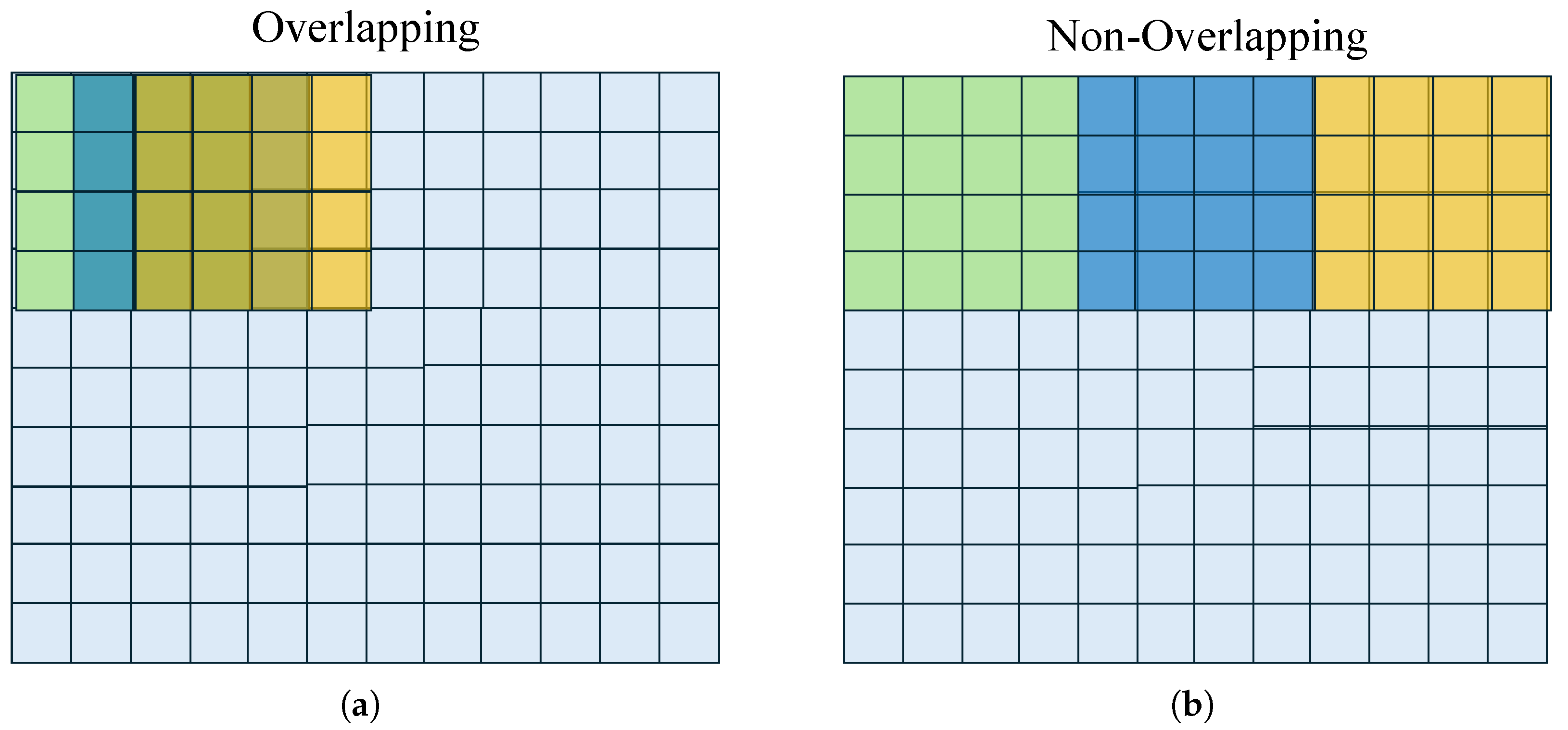
In ViT architectures, the patch embedding stem is typically implemented using a convolutional layer with a kernel size of $4\times 4$ and a stride of 4, generating non-overlapping patches while reducing computational resources. Figure 4 compares two sampling schemes: an overlapping configuration, in which the stride is smaller than the filter size, and a non-overlapping configuration, where the stride equals the filter dimensions. Hence, the patch embedding function is expressed as

$$y=\mathrm{Conv}2\mathrm{D}(x,\mathrm{k}=4,\mathrm{s}=4).$$

(4)

3.2. Gaussian Error Linear Units (GELUs)

The activation function is a key architectural hyperparameter because it introduces the non-linearity required for effective hierarchical feature extraction in CNNs. In Vision Transformer (ViT) architectures, the Gaussian error linear unit (GELU) has been broadly adopted [54]. Formally, the GELU function is defined as

$$\mathrm{GELU}\left(z\right)=z\mathrm{\Phi }\left(z\right),$$

(5)

where $\mathrm{\Phi }\left(z\right)$ denotes the cumulative distribution function (CDF) of the standard Gaussian variable. Since the Gaussian CDF has no closed form, an efficient and practical approximation is used in implementations:

$$\mathrm{\Phi }\left(z\right)={\displaystyle \frac{1}{\sqrt{2\pi }}}{\int }_{-\infty }^z{e}^{-{\displaystyle \frac{1}{2}}{t}^2}dt\approx {\displaystyle \frac{1}{2}}\left(1+tanh\left(\sqrt{{\displaystyle \frac{2}{\pi }}}(z+0.044715z^3)\right)\right).$$

(6)

GELU is smooth, non-monotonic, and fully differentiable, offering a closer approximation to the rectified linear unit (ReLU) while eliminating its piecewise linear discontinuity, leading to more stable gradient propagation and providing implicit weight regularization [55]. These characteristics have contributed to the widespread adoption of the GELU function in robust neural network architectures such as ViT, BERT, and GPT. Figure 5 illustrates the smooth behavior of GELU compared to the abrupt traditional piecewise ReLU activation function.

Overall, GELU preserves the gating behavior of ReLU by allowing positive inputs to pass while softly attenuating negative ones. Hence, it introduces a smooth and fully differentiable curve around zero. Unlike the tanh and $\mathrm{sigmoid}$ activations, whose outputs saturate for large-magnitude inputs, diminishing gradient strength, GELU exhibits milder gradient decay. This balance between smoothness and gradient continuity has made GELU a preferred activation in modern deep learning architectures.

3.3. Layer Normalization

Batch normalization (BN) has become a staple in modern CNNs because it standardizes layer activations, mitigates internal covariate shift, and thus smooths the loss landscape, enabling faster and more stable backpropagation convergence [56]. However, small or highly variable mini-batch sizes can produce noisy estimates, leading to numerical instability that may hinder learning and ultimately reduce final accuracy [57].

In contrast, layer normalization (LN) circumvents this limitation by computing the mean and variance for each sample over its feature channels. Because normalization constants are independent of the batch dimension, LN remains effective even with tiny batches, making it particularly suitable for memory-constrained training, recurrent and sequential architectures, and on-device or online inference scenarios [58,59]. Moreover, LN improves the numerical conditioning of the optimization problem. By rescaling activations within a standard or controlled range, the Jacobian’s singular values are kept near unity, stabilizing gradients and enabling the use of larger learning rates without divergence [56].

Furthermore, LN is the standard normalization method in Transformer architectures, where its sample-wise operation accommodates variable-length sequences and prevents inter-sample coupling [60]. For an input vector $\mathbf{X}=\left[x_{n,c,h,w}\right]\in {\mathbb{R}}^{N\times C\times H\times W}$, where $n\in \{1,\dots ,N\}$ indexes the mini-batch sample, $c\in \{1,\dots C\}$ indexes the feature channels, and $(h,w)$ denote spatial coordinates; LN computes, for each sample n, the mean and variance across all feature dimensions as follows:

$${\mu }_{n,c}={\displaystyle \frac{1}{N}}\sum _{h=1}^H\sum _{w=1}^W{x}_{n,c,h,w},{\sigma }_{n,c}^2={\displaystyle \frac{1}{N}}\sum _{h=1}^H\sum _{w=1}^W{\left(x_{n,c,h,w}-{\mu }_{n,c}\right)}^2,$$

(7)

where $N=H\times W$. The normalized activation map is obtained using the pseudo z-score transform:

$$y_{n,c,h,w}={\gamma }_c{\displaystyle \frac{x_{n,c,h,w}-{\mu }_{n,c}}{\sqrt{{\sigma }_{n,c}^2+\epsilon }}}+{\beta }_c,$$

(8)

where $ϵ>0$ ensures numerical stability, and the learnable parameters ${\gamma }_c$ (scale) and ${\beta }_c$ (bias), one pair per channel, restore the layer’s expressive power.

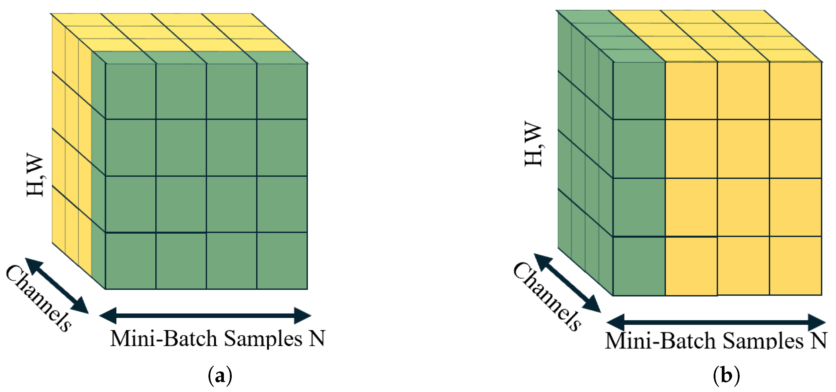
Figure 6 provides a visual comparison of batch normalization and layer normalization. In this 3D representation, the x-axis indexes the mini-batch samples, the y-axis corresponds to the channel dimension, and the z-axis represents the image dimensions.

3.4. Multi-Feature Stem Module

Medical images exhibit low contrast, inherent noise, and acquisition-related artifacts, which can lead to blurred or ambiguous boundaries. Moreover, due to the heterogeneous nature of the neoplasm, extracting multi-scale features is essential for accurate representation and analysis [61]. Feature maps generated by kernels of different sizes are fused to exploit complementary receptive fields. This multi-scale aggregation enriches both fine-grained details and global context, producing a more discriminative representation for post-processing.

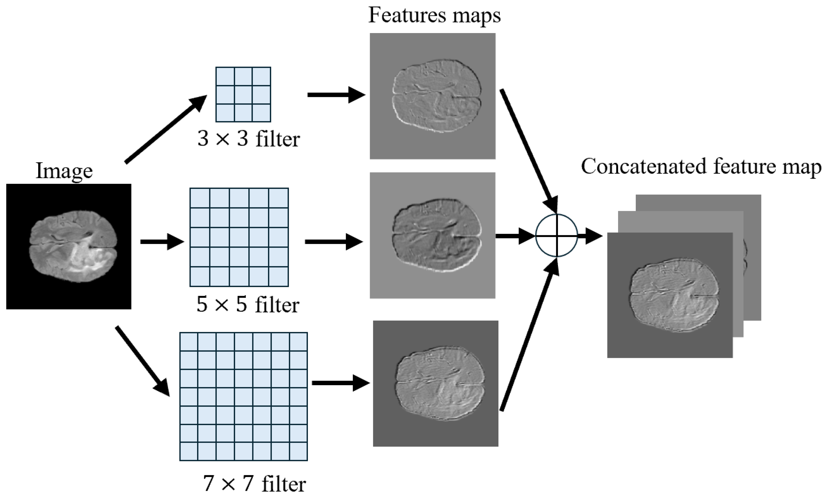
Figure 7 illustrates the multi-scale feature extraction stage, in which convolutional branches with kernels of different sizes process the image. Next, the extracted feature maps are concatenated to form a fused multi-scale representation.

3.5. Reverse Attention

A ResNet transmits information across layers through skip connections. For instance, in a ResNet model, input features are propagated to subsequent layers via an identity skip connection, thereby preserving low-level information and mitigating the vanishing gradient problem [62]. However, directly propagating features from the input to the output inevitably carries along background noise. Reverse Attention (RA) addresses this issue by exploiting high-level semantic cues to impose top-down (reverse) supervision on low-level representations, thereby suppressing irrelevant background regions and focusing on salient features [63]. The mathematical definitions of the operators involved in the RA module are as follows:

$$\begin{array}{cc}\hfill M_k^{RA}& =s\left(up\left(F_{k+1}\right)\right),\hfill \\ \hfill {\tilde{M}}_k^{\mathrm{RA}}& =\mathbf{1}-M_k^{\mathrm{RA}},\hfill \\ \hfill F_k^{RA}& ={\tilde{M}}_k^{RA}\otimes F_k,\hfill \end{array}$$

(9)

where $s(·)$ is the sigmoid function, and ⊗ is the Hadamard product. $M_k^{\mathrm{RA}}$ represents the foreground probability map; conversely, its binary complement ${\tilde{M}}_k^{\mathrm{RA}}$ controls the network’s attention in low-confidence regions, thereby improving boundary refinement. Here, the upsampling operator $up(·)$ adjusts the spatial resolution of the deeper feature map $F_{k+1}$ to match that of the shallower map $F_k$, thus ensuring proper feature alignment prior to fusion.

Figure 8 illustrates how the RA module operates: it first processes the subsequent feature map using a sigmoid function to produce a probabilistic activation map. This activation map is then inverted to highlight background regions and used as a Reverse Attention mask. These background activations are subsequently suppressed via element-wise fusion with the original input feature map. This approach enhances the focus on salient structures while mitigating the influence of irrelevant background information.

3.6. Inverted Residual and Linear Bottlenecks

Residual blocks have previously been used in medical imaging to reduce the vanishing gradient problem in convolutional network models [65]. In these architectures, residual blocks are linked by shortcut connections that allow inputs to bypass weighted activations and propagate information directly to subsequent layers. By facilitating gradient flow through many layers during backpropagation, these connections alleviate optimization difficulties in dense networks and can substantially improve predictive performance [65]. The standard ResNet bottleneck (Figure 9a) first reduces channel dimensionality via a standard convolutional layer and then expands it again to restore dimensionality. In contrast, the inverted residual bottleneck (Figure 9b) broadens the channels, first expanding the number of channels, applying depthwise convolutions, and subsequently projecting them back to a lower-dimensional space, placing the bottleneck at the end of the block. This strategy improves computational efficiency by reducing the number of operations compared to applying convolutions across a large number of channels [66].

3.7. AdamW Optimizer

Recent theoretical work by Zhou et al. [67] provides the first unified analysis of AdamW, clarifying how the decoupled weight-decay term influences both the optimization dynamics and empirical performance. The parameters updated in AdamW are formally defined as follows:

$$\begin{array}{cc}\hfill m_t& ={\beta }_1{m}_{t-1}+(1-{\beta }_1)g_t,\hfill \\ \hfill v_t& ={\beta }_2{v}_{t-1}+(1-{\beta }_2)g_t^2,\hfill \\ \hfill {\widehat{m}}_t& ={\displaystyle \frac{m_t}{1-{\beta }_1^t}},\hfill \\ \hfill {\widehat{v}}_t& ={\displaystyle \frac{v_t}{1-{\beta }_2^t}},\hfill \\ \hfill {\theta }_t& ={\theta }_{t-1}-{\displaystyle \frac{\alpha }{\sqrt{{\widehat{v}}_t}+ϵ}}\left({\widehat{m}}_t+\lambda {\theta }_{t-1}\right),\hfill \end{array}$$

(10)

where $m_t$ and $v_t$ denote the exponentially weighted first- and second-moment estimates of the stochastic gradient $g_t$, respectively; ${\beta }_1$ and ${\beta }_2$ are their corresponding decay factors; and ${\widehat{m}}_t$ and ${\widehat{v}}_t$ represent the bias-corrected forms of $m_t$ and $v_t$. Moreover, $\alpha$ specifies the base learning-rate hyperparameter, $ϵ$ is a small positive constant introduced to ensure numerical stability, and $\lambda$ determines the strength of the decoupled weight-decay regularizer.

Unlike the original Adam algorithm, which couples ${\ell }_2$ regularization to the gradient update, AdamW applies weight decay directly to the parameters. This explicit decoupling isolates the regularization effect from the adaptive update, resulting in more stable convergence and improved generalization. Thus, weight decay can be interpreted as an ${\ell }_2$ regularization term with coefficient $\lambda$ in the following augmented loss function:

$${\mathcal{L}}_{\mathrm{total}}\left(\mathbf{w}\right)={\mathcal{L}}_{\mathrm{data}}\left(\mathbf{w}\right)+{\displaystyle \frac{\lambda }{2}}{\parallel \mathbf{w}\parallel }_2^2,$$

(11)

where ${\mathcal{L}}_{\mathrm{data}}\left(\mathbf{w}\right)$ is the original task loss. Taking the gradient of ${\mathcal{L}}_{\mathrm{total}}\left(\mathbf{w}\right)$ and applying a learning-rate step yields the classic shrinkage update,

$${\mathbf{w}}_{t+1}=(1-\alpha \lambda ){\mathbf{w}}_t-\alpha {\nabla }_{\mathbf{w}}{\mathcal{L}}_{\mathrm{data}}\left({\mathbf{w}}_t\right),$$

(12)

which contracts each weight by a factor of $(1-\alpha \lambda )$ before the data-driven adjustment. In AdamW, this decay term is explicitly decoupled from the adaptive moment estimation, as shown in the final update Equation (12). This decoupling ensures that regularization does not interfere with adaptive learning dynamics, leading to more stable convergence and better generalization.

3.8. Loss Function

In medical imaging, the region of interest occupies only a small fraction of the image, producing a pronounced class imbalance that hinders optimization and often results in biased predictions and degraded segmentation quality [68]. Two complementary loss functions are routinely used for semantic segmentation. The former commonly used loss is binary cross-entropy (BCE), which measures the per-pixel discrepancy between predicted probabilities and ground-truth labels [69]. The BCE loss function is formally defined by

$${\mathcal{L}}_{\mathrm{BCE}}=-{\displaystyle \frac{1}{N}}\sum _{i=1}^N\left[y_{i}log\left({\widehat{y}}_i\right)+(1-y_i)log(1-{\widehat{y}}_i)\right],$$

(13)

where N denotes the number of pixels, $y_i\in [0, 1]$ represents the ground-truth label, and ${\widehat{y}}_i\in [0, 1]$ is the predicted probability for the positive class. BCE performs satisfactorily when classes are balanced. However, under severe class imbalance, it treats pixels independently, potentially overemphasizing the background class.

The latter, the Dice coefficient, is widely adopted for training and evaluating segmentation models on imbalanced segmentation tasks, emphasizing region overlap rather than per-pixel counts [70]. The Dice loss function is expressed as

$${\mathcal{L}}_{\mathrm{Dice}}=1-2{\displaystyle \frac{{\sum }_{i=1}^N{y}_i{\widehat{y}}_i+ϵ}{{\sum }_{i=1}^N{y}_i+{\sum }_{i=1}^N{\widehat{y}}_i+ϵ}}.$$

(14)

Therefore, in multi-class problems with severe class imbalance, such as BraTS, hybridizing loss functions can yield a more stable training process by using a robust optimization objective function. In the proposed hybrid loss function, BCE provides probability calibration while Dice offers overlap-oriented, i.e., balancing of strong localization gradients with regional stability. The composite loss function is mathematically described as follows:

$${\mathcal{L}}_{\mathrm{Hybrid}}=\alpha {\mathcal{L}}_{\mathrm{BCE}}+(1-\alpha ){\mathcal{L}}_{\mathrm{Dice}},$$

(15)

where $\alpha =0.5$ is chosen for the sake of equilibrium.

4. Materials and Methods

4.1. Brain Tumor Segmentation (BraTS) Dataset Description

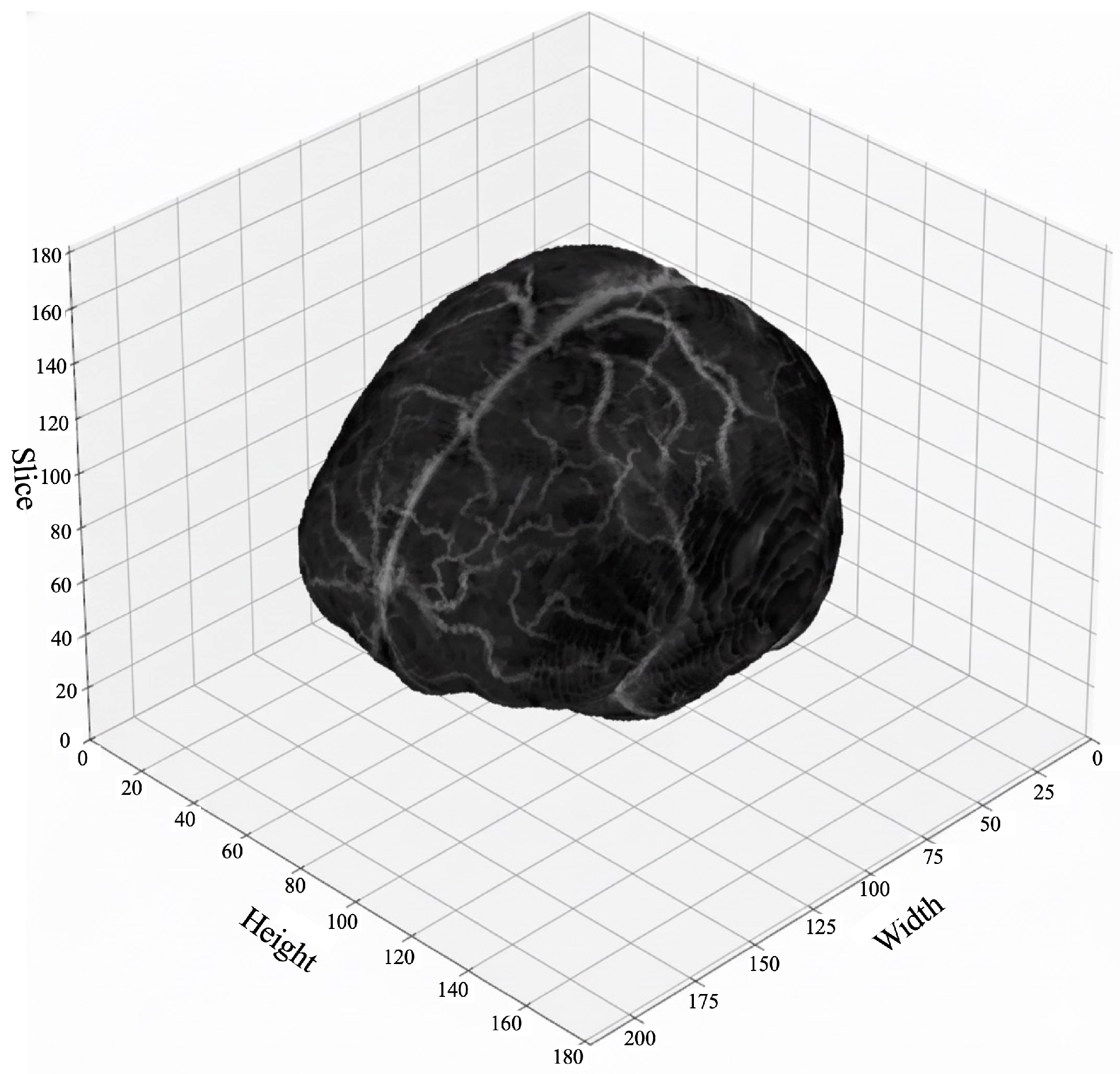
The BraTS dataset encompasses two complementary tasks: tumor segmentation and tumor classification. Both tasks rely on the same collection of multiparametric magnetic resonance imaging (mpMRI) data, provided as 3D volumes in the Neuroimaging Informatics Technology Initiative (NIfTI) format (*.nii). Each 3D volume comprises 155 contiguous axial slices, forming a three-dimensional array of size $height\times width\times depth$.

Table 2. A comparative analysis of the structural frameworks of each dataset, along with the corresponding image dimensions.

Dataset	Image	Training Set Size	Testing Set Size
BraTS 2021 [30]	$512\times 512\times 155$	277	120
BraTS 2023 [31]	$512\times 512\times 155$	840	360
BraTS 2024 [32]	$512\times 512\times 155$	840	360

summarizes the composition of the BraTS 2021, 2023, and 2024 datasets, following a 70/30 train–test split protocol.

Note that the number of published studies using BraTS 2024 is significantly lower than those using 2021 or 2023. Each element of this array represents a volumetric pixel element (voxel), thereby encoding 3D spatial information along the cranio-caudal extent of the brain, as shown in Figure 10.

4.2. Data Preprocessing

As the images are acquired as 3D volumes, a single slice is selected for fast processing. Among individual MRI modalities, T2-weighted images yielded the most consistent contrast for tumor-core delineation under the current single-slice extraction pipeline. However, FLAIR remains critical for characterizing peritumoral edema and diffuse infiltration; certainly, its integration into future multimodal fusion pipelines may further improve sensitivity to non-enhancing regions.

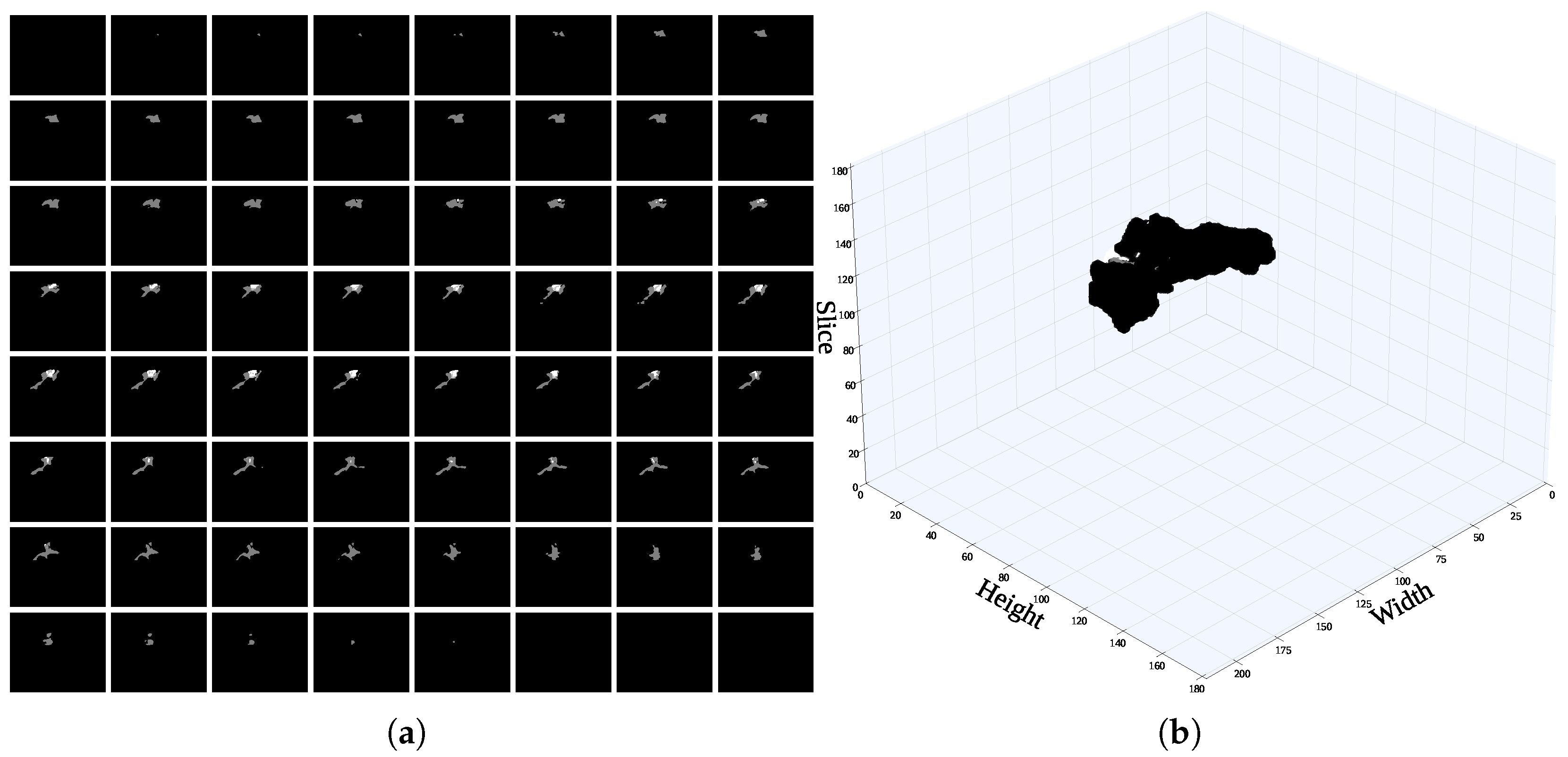
In this study, the optimal slice from the T2-weighted MRI images is selected using the corresponding ground truth as a reference. Specifically, an adaptive selection method extracts the slice with the highest tumor content, quantified as the binary whole-tumor (WT) region in the ground-truth mask. For instance, Figure 11 shows that the slice with the largest tumor content is not necessarily the central slice; in this case, the optimal slice index was 78. Additionally, all images were normalized using min–max scaling to the $[0, 1]$ range, defined as

$$\widehat{I}={\displaystyle \frac{I-min\left(I\right)}{max\left(I\right)-min\left(I\right)}}\in [0, 1],$$

(16)

Let $I\in {\mathbb{R}}^{D\times H\times W}$ denote the original 3D image and $I_{\mathrm{mask}}\in {\{0, 1\}}^{D\times H\times W}$ its corresponding binary tumor mask, where $D=155$ is the number of slices. To identify the slice containing the largest tumor region, the tumor content for each slice $S_d\in \{1,\dots ,D\}$ is computed as

$$T\left(S_d\right)=\sum _{h=1}^H\sum _{w=1}^W{I}_{\mathrm{mask}}(S_d,h,w).$$

(17)

The slice index with the maximum tumor content is selected by optimizing (17) as follows:

$$S_d^{\ast }=\underset{S_d\in \{1,\dots ,D\}}{arg\; max}T\left(S_d\right),$$

(18)

Finally, the corresponding best 2D slice from the original volume is extracted as

$$I_{\mathrm{best}}=I(S_d^{\ast },:,:)$$

(19)

where $I_{\mathrm{best}}$ denotes the most informative axial slice in terms of tumor burden, which is then used for further analysis.

4.3. Comprehensive Framework

ConvNeXt, introduced by Meta AI (formerly Facebook AI Research) in 2022 [66], is a CNN architecture inspired by the Swin Transformer, incorporating depthwise convolution and an inverted bottleneck design [71]. ConvNeXt was designed to modernize CNNs and demonstrate their competitiveness with ViTs in terms of accuracy and scalability [66]. Design principles inspired by Transformers, including layer normalization, simplified architecture, and scalable configurations, were incorporated into ConvNeXt to enable CNNs to achieve state-of-the-art performance in image classification, segmentation, and object detection. Computational efficiency and compatibility with standard hardware were maintained, positioning ConvNeXt as a robust and efficient alternative for vision tasks.

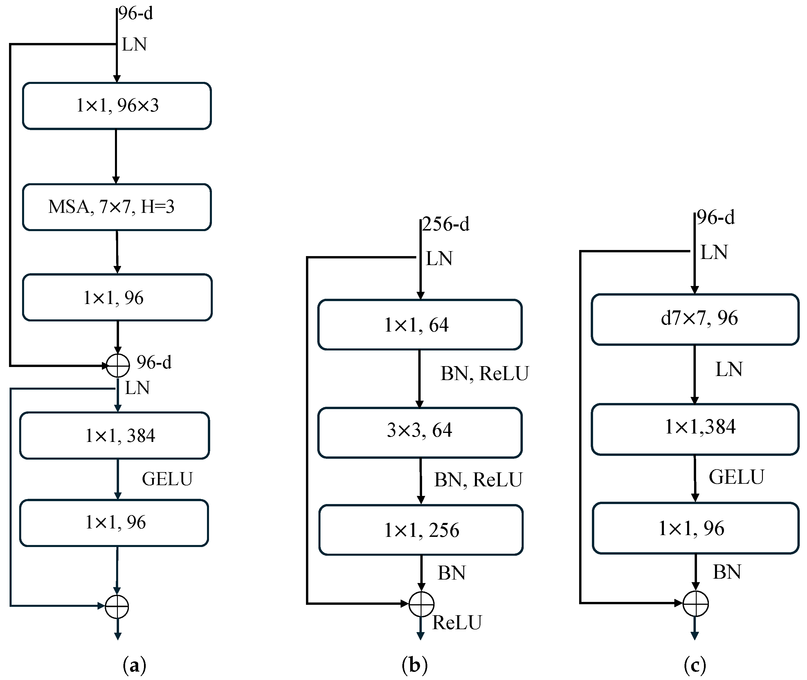
ConvNeXt blocks are typically more efficient than ResNet and Swin Transformer blocks due to substituting heavy attention and dense convolutions with depthwise separable operations and simplified normalization, thereby reducing both computational costs and memory usage. Figure 12 compares the functional blocks of the Swin Transformer, ResNet, and ConvNeXt architectures.

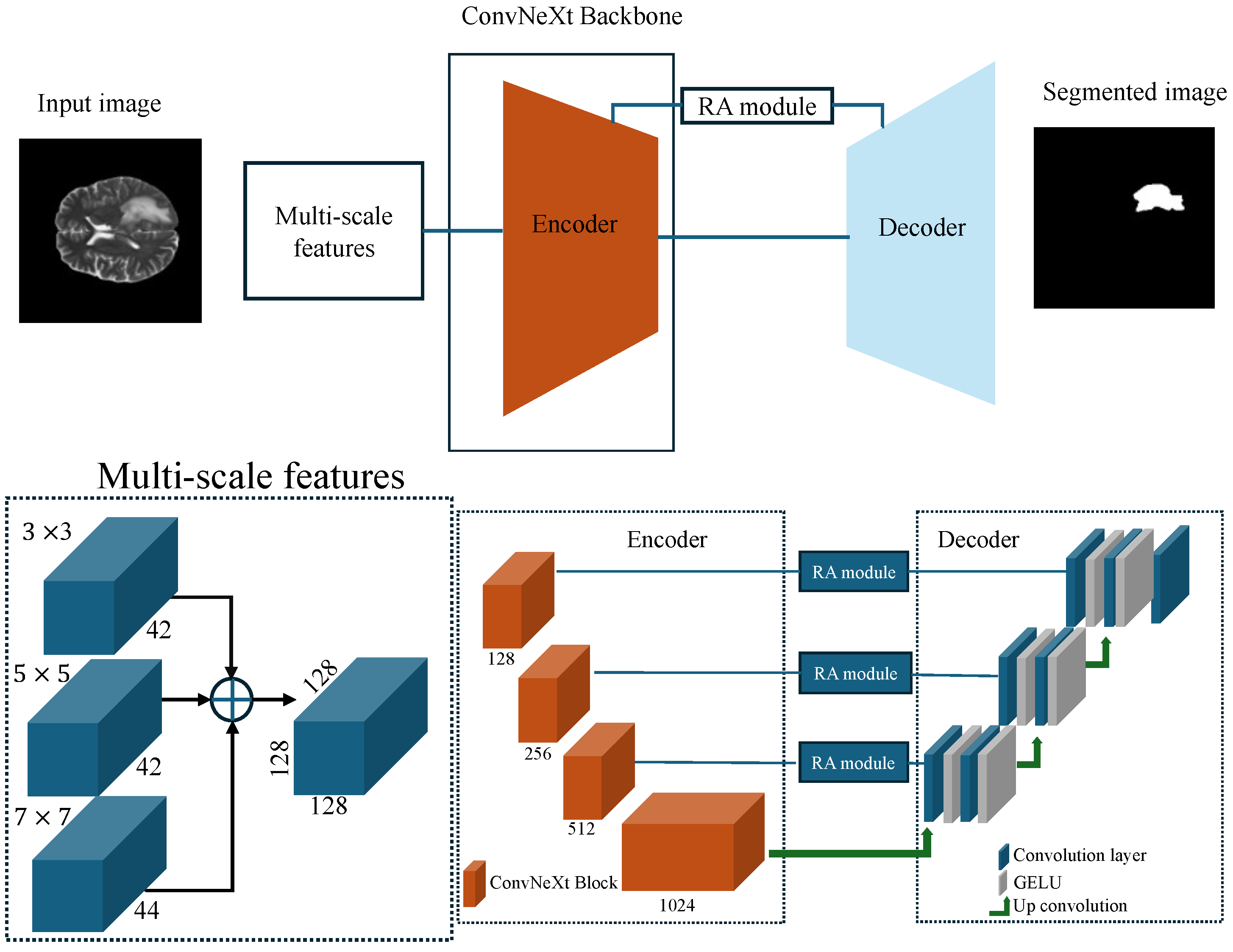
Figure 13 depicts the complete proposed architecture, consisting of a modified UNet with an enhanced encoder backbone and additional modules integrated both within and outside the model. As a preprocessing step, the input MRI slice is passed through a multi-scale feature extraction stem comprising three parallel convolutional branches with kernel sizes of $3\times 3$, $5\times 5$, and $7\times 7$, producing 42, 42, and 43 output channels, respectively. The branch depths are chosen to match the ConvNeXt input width of 128 channels. Functionally, the $3\times 3$ branch emphasizes fine-grained structures such as tumor borders, small enhancing cores, and thin vascular cues. In contrast, the $5\times 5$ and $7\times 7$ branches capture mid-scale context and broader peritumoral patterns, including edema and infiltrative regions. The branch outputs are concatenated along the channel dimension, then normalized and activated to yield a compact, multi-scale embedding. This design expands the effective receptive field early in the pipeline without excessive depth, improves robustness to variability in lesion size, shape, and intensity, and provides richer features to the downstream encoder–decoder [66].

Subsequently, the network adopts a UNet architecture with a ConvNeXt encoder backbone and a decoder that mirrors the encoder’s depth. ConvNeXt provides a strong hierarchical representation through depthwise convolutions with large effective receptive fields, pointwise channel expansions that enrich feature capacity, layer normalization for stable optimization, and residual pathways that preserve information flow. Standard UNet skip connections are maintained to recover fine spatial detail in the decoder, and a lightweight Reverse Attention unit modulates each skip connection to limit background leakage and emphasize boundary-adjacent errors.

4.4. Implementation Details

The experiments were conducted in Python using the PyTorch (ver. 2.5.1) framework, which supports CUDA 11.8 and was used to accelerate model training and inference. The device features an NVIDIA RTX 3070 Ti graphics card with 8 GB of GDDR6X VRAM and 6144 CUDA cores, as well as an Intel Core i7 processor.

The nibabel library (ver. 5.3.2) was used to access the medical images. No data augmentation was employed to avoid introducing additional variability. The training stage was run for 500 epochs, during which the model’s best weights were stored to mitigate overfitting. Each epoch of training used mini-batches of four images, with all computations executed in single-precision 32-bit floating-point (FP32). Additional training hyperparameter details are summarized in

Table 3. Hyperparameter settings used in all experiments.

Hyperparameter	Value
Optimizer	AdamW
Learning rate	$1\times {10}^{-3}$
Weight decay	$1\times {10}^{-4}$
Loss	$0.5{\mathcal{L}}_{BCE}+0.5{\mathcal{L}}_{DSC}$

. To mitigate overfitting, the checkpoint with the best validation performance was retained, and an early-stopping criterion (patience = 20 epochs) was set to stop training once validation metrics stagnated. The source code is available at https://github.com/fdhernandezgutierrez/MultiscaleConvNeXtMRI (accessed on 24 December 2025).

5. Numerical Results

5.1. Evaluation Metrics

This section defines the quantitative metrics that underlie the evaluation strategy and explains how they are used to benchmark the proposed model against the state of the art. The analysis relies on the Dice coefficient (DSC), the intersection over union (IoU), precision, sensitivity, specificity, accuracy, and inference time, thereby capturing both the segmentation accuracy and computational efficiency.

5.1.1. Dice Similarity Coefficient

The Dice similarity coefficient (DSC) measures the overlap between two segmented images, specifically in the context of semantic segmentation, ranging from 0 to 1 [72]. This process is performed by overlapping the pixels of the ground-truth image with those of the model-segmented image. The value ranges from 0 (no pixel overlap) to 1.0 (perfect segmentation); 0.5 indicates half-pixel overlap. The DSC metric is computed as follows:

$$\mathrm{DSC}=2{\displaystyle \frac{|A\cap B|}{\left|A\right|+\left|B\right|}},$$

(20)

where A is the mask of ground-truth segmentation, B is the model-predicted mask, $A\cap B$ denotes their intersection (the number of pixels common to both masks), and $\left|A\right|+\left|B\right|$ denotes the total number of foreground pixels in the mask of ground-truth A and the predicted mask B. Consider the identity $\left|A\right|+\left|B\right|=|A\cup B|+|A\cap B|$, where $|A\cap B|$ denotes the number of foreground pixels common to both images.

5.1.2. Intersection over Union

The intersection over union (IoU) quantifies the spatial agreement between two segmentation images by comparing their shared region (intersection) to their total combined extent (union) [72]. It is defined as

$$\mathrm{IoU}={\displaystyle \frac{|A\cap B|}{|A\cup B|}},$$

(21)

where A denotes the ground truth, B the predicted segmentation, $|A\cap B|$ is the area of their intersection, and $|A\cup B|$ is the area of their union. The IoU ranges from 0 to 1, attaining a value of 1 only when the predicted mask perfectly coincides with the reference.

5.1.3. Hausdorff Distance

The Hausdorff distance (HD) quantifies the maximum boundary discrepancy between the ground truth and the predicted segmentation, emphasizing worst-case boundary errors and outliers. It is defined as follows:

$$\mathrm{HD}(A, B)=max\left\{\underset{a\in A}{max}\underset{b\in B}{min}d(a, b),\underset{b\in B}{max}\underset{a\in A}{min}d(b, a)\right\},$$

(22)

where A is the ground-truth mask, B is the predicted mask, and $d(a, b)={\parallel a-b\parallel }_2$ denotes the Euclidean distance between points a and b. Here, min selects, for each point in one set, the distance to its closest point in the other set, whereas max returns the largest of these closest-point distances, representing the worst-case boundary mismatch.

5.1.4. Precision

Precision quantifies the reliability of true-positive predictions of a segmentation model at the pixel level. Let $TP$ be the set of pixels that the model detects correctly and are labeled as tumors in the ground-truth mask, and let $\mathrm{FP}$ be the set of pixels that the model misclassifies as tumors but are labeled as background in the ground-truth mask [73]. Formally, this metric is defined as

$$\mathrm{Precision}={\displaystyle \frac{\left|TP\right|}{\left|TP\right|+\left|FP\right|}},$$

(23)

where $|·|$ denotes the cardinality of a set of pixels. This metric represents the fraction of pixels that the model labels as tumors that are truly tumors. The score ranges from 0 to 1 and attains a value of 1 only when the segmentation contains no false-positive pixels.

5.1.5. Sensitivity

Sensitivity, also known as recall, measures the completeness of the tumor detection model. Let $TP$ denote the set of pixels that are tumors in both the prediction and the ground-truth mask, and let $FN$ denote the set of pixels that are tumors in the ground-truth mask but are missed by the model [24]. Formally, this metric is given by

$$\mathrm{Sensitivity}={\displaystyle \frac{\left|TP\right|}{\left|TP\right|+\left|FN\right|}},$$

(24)

Hence, recall represents the proportion of all ground-truth tumor pixels that the model successfully identifies. The value ranges from 0 to 1, attaining 1 only when segmentation produces no false-negative pixels.

5.1.6. Specificity

Specificity, also known as the true-negative rate, measures the model’s ability to reject non-tumor pixels correctly. Let $TN$ be the set of pixels correctly classified as background in both the prediction and the ground-truth mask. And, $FP$ is the set of pixels incorrectly labeled as tumors by the model but annotated as background in the ground truth [24]. Formally, it is denoted as

$$\mathrm{Specificity}={\displaystyle \frac{\left|TN\right|}{\left|TN\right|+\left|FP\right|}},$$

(25)

Thus, specificity expresses the proportion of all ground-truth background pixels that the model correctly identifies as background. The value ranges from 0 to 1, reaching 1 only when segmentation introduces no false-positive pixels.

5.1.7. Accuracy

Accuracy measures the proportion of pixels the model classifies correctly [73]. Formally,

$$\mathrm{Accuracy}={\displaystyle \frac{\left|TP\right|+\left|TN\right|}{\left|TP\right|+\left|TN\right|+\left|FP\right|+\left|FN\right|}},$$

(26)

Its value ranges from 0 to 1, attaining 1 only when the model makes no classification errors.

5.1.8. F1-Score

The F1-score is estimated by the harmonic mean of precision and recall, which is characterized by penalizing extreme measures in either component [74]. This metric is not symmetric with respect to the class labels because both precision and recall are computed relative to the class designated as positive. Consequently, in a setting with a large positive class and a classifier biased toward that majority, the F1-score can be high due to a large number of true positives; if the labels are inverted so that the majority becomes the negative class while the classifier remains biased toward it, the F1-score can become low, even though the data and class distribution are unchanged. For a binary classifier, the F1-score is defined as

$$\mathrm{F}1=2\times {\displaystyle \frac{\mathrm{Precision}\times \mathrm{Recall}}{\mathrm{Precision}+\mathrm{Recall}}}={\displaystyle \frac{2\times TP}{2\times TP+FP+FN}}.$$

(27)

5.2. Performance Evaluation and Ablation Study

Table 4. Averaged performance metrics obtained from three datasets.

Dataset	IoU	DSC	Sensitivity	Specificity	Accuracy	F1-Score
BraTS 2021	0.8200	0.9003	0.8836	0.9964	0.9881	0.9003
BraTS 2023	0.8592	0.9235	0.9037	0.9977	0.9904	0.9235
BraTS 2024	0.8575	0.9225	0.8989	0.9979	0.9903	0.9225

summarizes the model’s overall performance metrics achieved using the model and the applied fine-tuning procedure.

In addition,

Table 5. Comparison of different metrics for the Transformer models trained on the BraTS 2021 dataset.

Reference	IoU	DSC	HD	Sensitivity	Specificity	F1-Score
Andrade-Miranda et al. [33]	-	0.896	-	-	-	-
Chen and Yang [36]	-	0.9335	2.8284	-	-	-
Jia and Shu [37]	-	0.9257	-	-	-	-
Jiang et al. [38]	-	0.9183	3.65	-	-	-
Dobko et al. [42]	-	0.8496	3.37	-	-	-
Yang et al. [35]	-	0.8392	-	-	-	-
ZongRen et al. [39]	-	0.932	4.58	-	-	-
Lin et al. [41]	-	0.933	6.20	0.9334	-	-
UNet Baseline	0.7465	0.8535	40.30	0.8061	0.9961	0.8535
Proposed model	0.8122	0.8956	33.038	0.8761	0.9964	0.8956

provides a comparative overview of the proposed model and several state-of-the-art Transformer-based architectures evaluated on the BraTS 2021 dataset. Specifically, key segmentation metrics, including intersection over union (IoU), Dice similarity coefficient (DSC), Hausdorff distance (HD), sensitivity, specificity, and F1-score are reported to facilitate a comprehensive assessment.

Although the proposed model achieves a slightly lower DSC, 0.8956, than the top-performing models (up to 0.9335), it attains a competitive IoU of 0.8122, indicating substantial agreement with the ground-truth segmentation. Furthermore, the model demonstrates a high sensitivity of 0.8761 and an outstanding specificity of 0.9964, reflecting its ability to identify both tumor and non-tumor regions correctly. The reliable F1-score of 0.8956 confirms a balanced trade-off between precision and recall.

Likewise, as in

Table 6. Comparison of different metrics for models trained on the BraTS 2023 dataset.

Reference	IoU	DSC	HD	Sensitivity	Specificity	F1-Score
Nguyen-Tat et al. [75]	-	0.8820	-	-	-	-
Bhagyalaxmi and Dwarakanath [43]	-	0.9930	-	-	-	-
UNet baseline	0.7423	0.8490	53.93	0.8313	0.9947	0.8490
Our model	0.8592	0.9235	26.7270	0.9037	0.9977	0.92356

, the proposed model achieves an IoU of 0.8592 and a DSC of 0.9235 on the BraTS 2023 dataset. Although a previous study reported a higher DSC of 0.9930, the proposed approach achieves a very high specificity of 0.9977 while maintaining a sensitivity of 0.9037, indicating a strong ability to limit false positives without markedly compromising true-positive detection.

Furthermore, the F1-score of 0.9236 confirms a balanced precision–recall trade-off. In particular, several review articles do not report the IoU or other complementary metrics, so the primary basis for comparison remains DSC. Nevertheless, the additional indicators reported here underscore the practical reliability of the proposed method.

Table 7. Ablation study of different parameters on the BraTS datasets.

Dataset	Optimizer		Loss Functions			Evaluation Metrics
		Multi-Scale	BCE	DSC	RA	DSC	mIoU	Sensitivity	Specificity	Accuracy	F1-Score	HD
BraTS 2021	Adam	✓	✓	✓	✓	0.8924	0.8075	0.8749	0.9962	0.9875	0.8924	30.74
	Adam	✓	✗	✓	✓	0.8842	0.7983	0.8654	0.9959	0.9868	0.8842	54.44
	Adam	✓	✓	✗	✓	0.8815	0.7951	0.8622	0.9958	0.9865	0.8815	31.62
	AdamW	✓	✓	✗	✓	0.8956	0.8122	0.8761	0.9964	0.9878	0.8956	31.25
	AdamW	✓	✗	✓	✓	0.8867	0.8015	0.8689	0.9960	0.9870	0.8867	33.28
	AdamW	✓	✓	✓	✓	0.9003	0.8200	0.8836	0.9964	0.9881	0.9003	29.88
BraTS 2023	Adam	✓	✓	✗	✓	0.9213	0.8551	0.9157	0.9968	0.9899	0.9213	30.53
	Adam	✓	✗	✓	✓	0.8845	0.8006	0.8648	0.9960	0.9870	0.8845	50.74
	Adam	✓	✓	✓	✓	0.8871	0.8024	0.9380	0.9928	0.9981	0.8871	30.89
	AdamW	✓	✓	✗	✓	0.9078	0.8342	0.8929	0.9971	0.9893	0.9078	28.47
	AdamW	✓	✗	✓	✓	0.8931	0.8097	0.8710	0.9962	0.9876	0.8931	31.34
	AdamW	✓	✓	✓	✓	0.9235	0.8592	0.9037	0.9977	0.9904	0.9235	27.86
BraTS 2024	Adam	✓	✓	✗	✓	0.8561	0.7499	0.8036	0.9962	0.9811	0.8561	25.65
	Adam	✓	✗	✓	✓	0.8610	0.7528	0.8084	0.9960	0.9815	0.8610	37.74
	Adam	✓	✓	✓	✓	0.9094	0.8347	0.9100	0.9956	0.9866	0.9094	22.97
	AdamW	✓	✓	✗	✓	0.8483	0.7396	0.7787	0.9973	0.9808	0.8483	22.76
	AdamW	✓	✗	✓	✓	0.8519	0.7450	0.7855	0.9971	0.9810	0.8519	29.86
	AdamW	✓	✓	✓	✓	0.9225	0.8575	0.8989	0.9979	0.9903	0.9225	19.60

✓ indicates that this loss function is enabled, while ✗ means that the function has been disabled.

presents an ablation study for the results obtained with the multi-scale module; the Reverse Attention is held constant, indicating that the loss composition and the optimizer primarily determine performance.

Specifically, for BraTS 2021, the AdamW optimizer with a composite loss of hybrid BCE + DSC functions deliver the strongest results, with a DSC of 0.9003 and an mIoU of 0.8200, outperforming the AdamW variant without the DSC term, indicating that joint optimization consistently improves delineation. For BraTS 2023, in contrast, an optimizer–objective interaction emerges: the best configuration uses AdamW with a hybrid BCE + DSC loss function, achieving improved results: a DSC of 0.9235, an mIoU of 0.8592, a sensitivity of 0.9037, a specificity of 0.9977, and an F1 of 0.9236. It is noteworthy that AdamW benefits less from the composite objective and is more competitive than BCE alone.

5.3. Performance Estimation

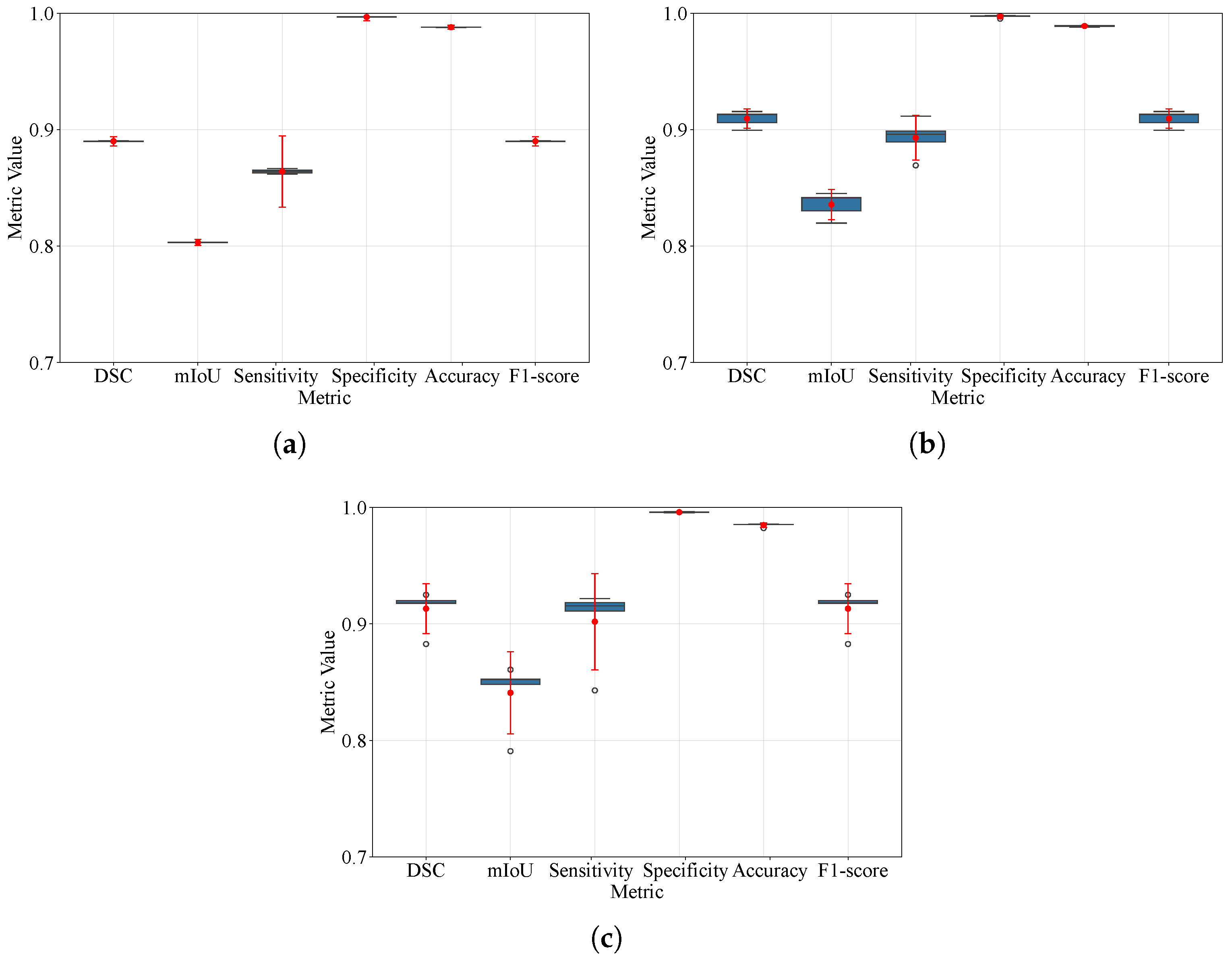
Figure 14 summarizes the distribution of segmentation metrics obtained under five-fold cross-validation on the BraTS 2024, BraTS 2023, and BraTS 2021 datasets. Figure 14c presents the five-fold performance for BraTS 2024 under AdamW and BCE-Dice loss. The results indicate uniformly strong and stable behavior. Specifically, specificity and accuracy exhibit near-ceiling medians with very narrow interquartile ranges and tight 95% confidence intervals, evidencing minimal dispersion. Likewise, the DSC and F1-score remain high with modest variability, whereas sensitivity is slightly lower yet still robust. By contrast, mIoU attains the lowest central tendency and displays the widest spread, consistent with its stricter penalization of boundary and small-structure errors.

Figure 14b shows the five-fold distributions for BraTS 2023 with AdamW and BCE-Dice loss, revealing consistently strong performance with limited variability across metrics. Specificity and accuracy are highly concentrated near the upper bound, with compressed interquartile ranges and narrow 95% confidence intervals, indicating minimal dispersion. DSC and F1-score also remain elevated with moderate spread, whereas sensitivity is comparatively lower yet still stable.

In contrast, mIoU shows the lowest central tendency and the broadest variability, as expected given its stricter penalization of boundary and small-structure errors. Figure 14a summarizes the five-fold performance on BraTS 2021 with AdamW and BCE–Dice loss. Overall, the distributions show high central tendency with limited dispersion across metrics. In particular, specificity and accuracy concentrate near the upper bound, with compressed interquartile ranges and narrow 95% confidence intervals, consistent with a mild ceiling effect. DSC and F1-score remain elevated with modest variability, whereas sensitivity is comparatively lower yet stable across folds. By contrast, mIoU displays the lowest central tendency and the broadest spread, reflecting its stricter penalization of boundary and small-structure errors. These visual findings are consistent with

Table 8. Performance on BraTS 2021, 2023, and 2024 (mean ± standard deviation) over 5-fold cross-validation.

Dataset	DSC	mIoU	Sensitivity	Specificity	Accuracy	F1-Score	Hausdorff
BraTS 2021	$0.8923\pm 0.076$	$0.849\pm 0.108$	$0.878\pm 0.109$	$0.989\pm 0.015$	$0.980\pm 0.014$	$0.842\pm 0.116$	$43.038\pm 16.138$
BraTS 2023	$0.885\pm 0.047$	$0.800\pm 0.069$	$0.840\pm 0.079$	$0.998\pm 0.001$	$0.987\pm 0.003$	$0.885\pm 0.047$	$34.816\pm 9.127$
BraTS 2024	$0.913\pm 0.017$	$0.841\pm 0.028$	$0.902\pm 0.033$	$0.996\pm 0.000$	$0.985\pm 0.001$	$0.913\pm 0.017$	$27.169\pm 7.005$

.

Table 9. Mean voxel-wise epistemic uncertainty on the BraTS test set, stratified by prediction outcome.

Dataset	Outcome	Definition	Mean Uncertainty
BraTS 2024	TP	Ground truth = 1, prediction = 1	0.00120
	FP	Ground truth = 0, prediction = 1	0.00880
	FN	Ground truth = 1, prediction = 0	0.01490
	TN	Ground truth = 0, prediction = 0	0.00260
BraTS 2023	TP	Ground truth = 1, prediction = 1	0.001330
	FP	Ground truth = 0, prediction = 1	0.004814
	FN	Ground truth = 1, prediction = 0	0.009376
	TN	Ground truth = 0, prediction = 0	0.001799
BraTS 2021	TP	Ground truth = 1, prediction = 1	0.003874
	FP	Ground truth = 0, prediction = 1	0.004664
	FN	Ground truth = 1, prediction = 0	0.003996
	TN	Ground truth = 0, prediction = 0	0.000601

presents the mean voxel-wise epistemic uncertainty for TP, FP, FN, and TN across the BraTS 2024, 2023, and 2021 test sets. In all three datasets, FN and FP voxels consistently exhibit higher epistemic uncertainty than TP and, in particular, TN voxels, indicating that the model is most uncertain precisely where misclassifications occur, while correctly identified background remains highly confident. These values are obtained using a Monte Carlo Dropout procedure at test time, in which dropout layers are kept active, multiple stochastic forward passes are performed, and the variance of the predictive probabilities across passes is used as a voxel-wise estimate of epistemic uncertainty before aggregating it by outcome type. This stratified analysis goes beyond global overlap metrics. It directly assesses the model’s reliability in clinically critical regions, providing a basis for uncertainty-aware visualization, expert review of high-uncertainty areas, and the design of future calibration or active learning strategies.

Table 10. Friedman test across BraTS 2021, BraTS 2023, and BraTS 2024 for the used segmentation metrics.

Metric	Friedman Statistic	p-Value
DSC	4.0	0.1353
mIoU	4.0	0.1353
Sensitivity	3.0	0.2231
Specificity	4.0	0.1353
Accuracy	1.0	0.6065
F1-score	4.0	0.1353

depicts the Friedman test used to assess potential performance differences across BraTS 2021, BraTS 2023, and BraTS 2024 for the main segmentation metrics, based on five-fold cross-validation. For DSC, mean IoU, specificity, and F1-score, the Friedman statistic was 4.0 (p = 0.1353), while sensitivity and accuracy yielded statistics of 3.0 (p = 0.2231) and 1.0 (p = 0.6065), respectively. In all cases, the p-values were clearly above the conventional 0.05 threshold: the null hypothesis of no performance difference among the three BraTS editions cannot be rejected. These findings indicate that the proposed model achieves comparable segmentation quality across BraTS 2021, 2023, and 2024, without evidence of systematic degradation or overfitting to a specific cohort.

Table 11. Slice-level failure mode analysis stratified by tumor size on the BraTS 2021, 2023, and 2024 test sets. Tumor size is defined as the number of ground-truth tumor pixels per slice. For each dataset, small, medium, and large groups correspond to the lower, middle, and upper thirds of the tumor-size distribution, with thresholds set at the 33rd and 66th percentiles. The last column reports the mean number of large false-negative (FN) clusters per slice, where a large FN cluster is defined as a connected component containing at least 100 misclassified tumor pixels.

Dataset	Size Class	# Slices	Dice (Mean ± Std)	Mean # Large FN Clusters
BraTS 2021	Small	63	0.873 ± 0.100	1.79
	Medium	62	0.908 ± 0.062	2.61
	Large	64	0.919 ± 0.058	3.48
BraTS 2023	Small	30	0.917 ± 0.048	1.43
	Medium	30	0.926 ± 0.065	1.93
	Large	31	0.956 ± 0.020	2.48
BraTS 2024	Small	10	0.933 ± 0.026	1.70
	Medium	10	0.946 ± 0.013	1.70
	Large	10	0.925 ± 0.065	2.90

summarizes a slice-level, DBSCAN-based cluster-wise failure mode analysis stratified by tumor size across the BraTS 2021, 2023, and 2024 test sets, revealing a consistent dependence of segmentation performance on lesion extent. For BraTS 2021 and BraTS 2023, the mean DSC increases monotonically from small to large tumors ($0.873\pm 0.100$ to $0.919\pm 0.058$ in 2021 and $0.917\pm 0.048$ to $0.956\pm 0.020$ in 2023), indicating that larger tumors are segmented more accurately and with lower variability. In contrast, small lesions constitute a more challenging and unstable regime. A similar pattern is observed for BraTS 2024 between small and medium lesions ($0.933\pm 0.026$ versus $0.946\pm 0.013$), while large tumors exhibit a slightly reduced Dice score ($0.925\pm 0.065$), which may reflect the limited number of slices per group and increased heterogeneity in this cohort rather than a systematic degradation of performance. In parallel, the mean number of large FN clusters, defined as spatially coherent regions of missed tumor voxels identified via DBSCAN, tends to increase with tumor size. In the three datasets this value is from 1.79 to 3.48 in BraTS 2021, from 1.43 to 2.48 in BraTS 2023, and from 1.70 to 2.90 in BraTS 2024, suggesting that larger lesions, despite achieving higher global overlap, frequently contain multiple localized regions that remain under-segmented. By contrast, small tumors present fewer large FN clusters in absolute terms. However, they are associated with lower DSCs and larger standard deviations, implying that missing one or two compact regions can represent a substantial fraction of the total lesion burden and therefore has a disproportionately negative impact on performance.

5.4. Computational Efficiency Analysis

Table 12. Computational efficiency analysis of the proposed model.

Model	Parameters	FLOPs	Inference (Mean ± Std)
	M = ${\mathbf{10}}^{\mathbf{6}}$	G = ${\mathbf{10}}^{\mathbf{9}}$	FPS	Latency (ms/Image)
UNet Baseline	31.38 M	97.70 G	9.03 ± 0.3006	110.8895 ± 3.5383
Proposed model	100.38 M	111.21 G	59.92 ± 0.3485	16.8065 ± 0.0968

provides a concise computational efficiency analysis of the proposed model and the UNet base. Although the proposed model has a larger capacity (100.38 M parameters, corresponding to approximately 0.40 GB in 32-bit floating-point format) and a slightly higher computational cost (111.21 G FLOPs compared to 97.7 G FLOPs for the baseline), it achieves substantially faster inference. Specifically, the proposed model achieves 59.92 ± 0.35 FPS (16.81 ± 0.10 ms per image), while the UNet baseline achieves 9.03 ± 0.30 FPS (110.88 ± 3.80 ms per image), resulting in approximately 6.6 times higher throughput and lower latency.

5.5. Segmentation Results

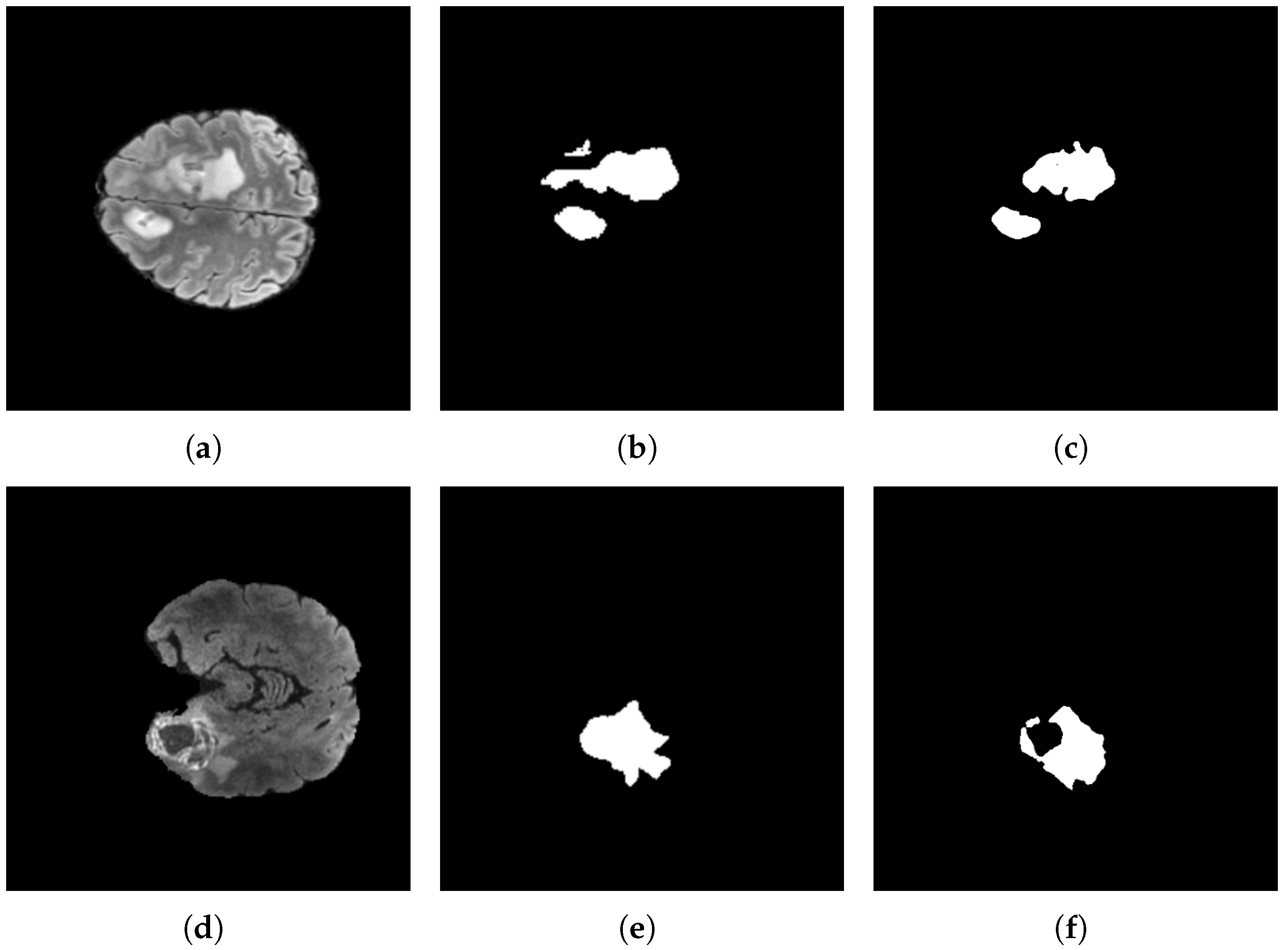
This section provides the representative WT segmentations using BraTS 2021, 2023, and 2024. The examples show comprehensive lesion coverage, well-defined boundaries, and robustness across scanners and acquisition protocols, with consistent performance under diverse anatomical presentations and imaging conditions. The segmentation quality confirms the effectiveness of the final model configuration, which was determined by the ablation analysis that quantifies the contributions of the multi-scale backbone, the spatial latent module, RA-guided skip connections, and the ${\mathcal{L}}_{Hybrid}$ loss function.

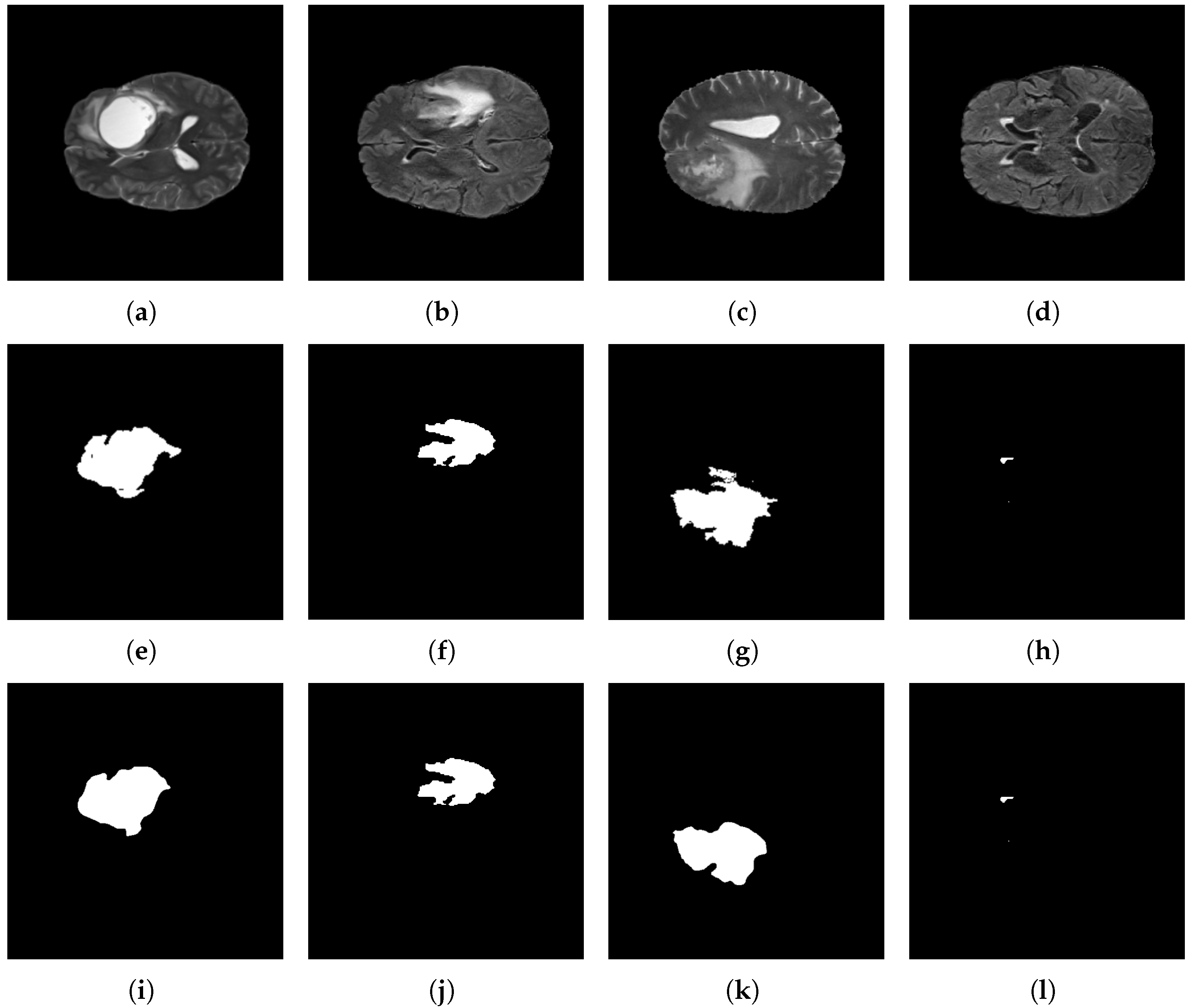
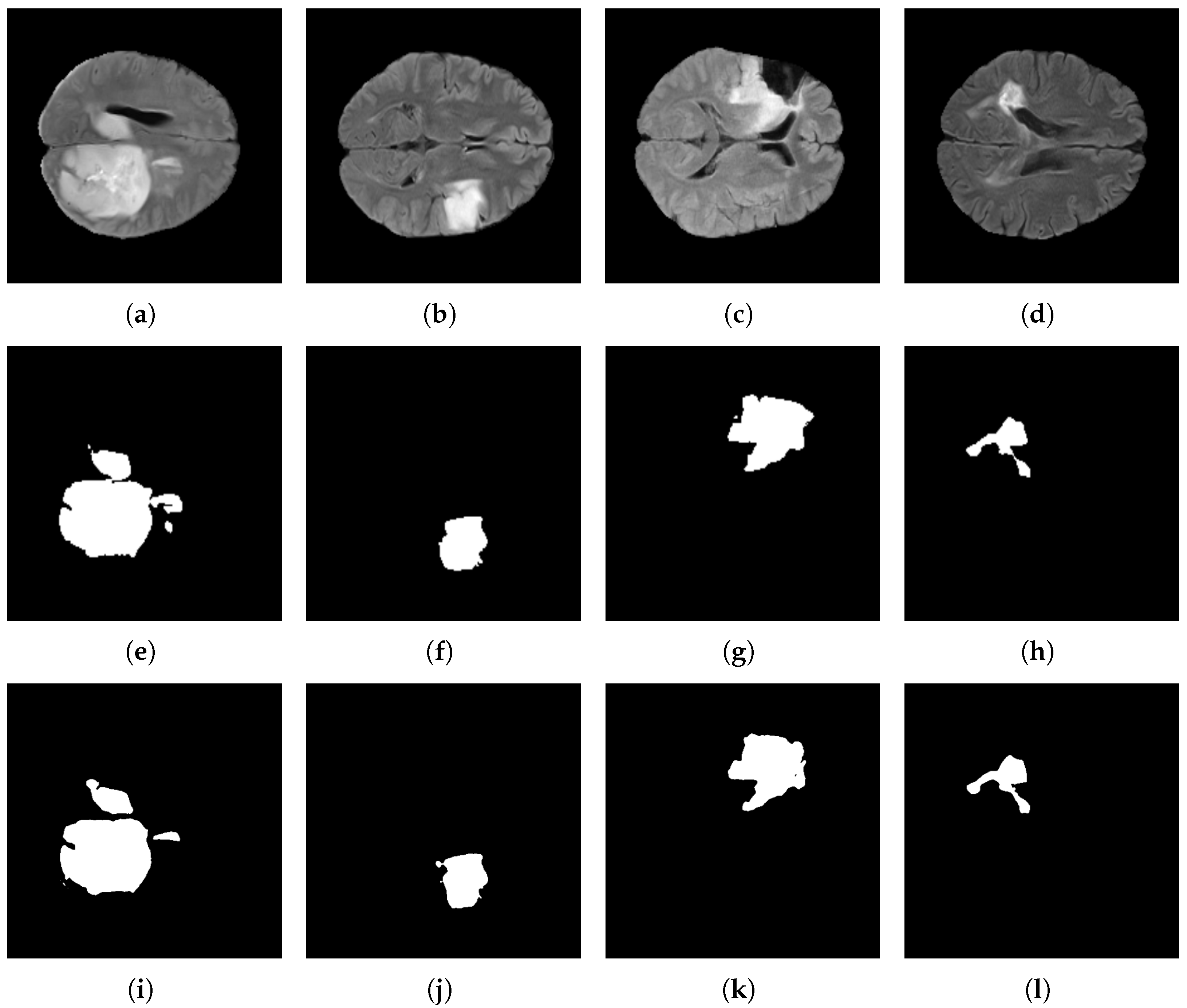
Figure 15 depicts the segmentation results for the BraTS 2021 dataset. The first row shows the original input images. The second row displays the corresponding ground-truth masks, while the third row illustrates the predictions generated by the proposed model.

Figure 15e shows a tumor with a rounded morphology; correspondingly, the model completely delineates it in Figure 15i, preserving a smooth boundary. By contrast, Figure 15f shows a spiculated contour with sharp protrusions, and the model accurately captures these border irregularities in Figure 15j without excessive smoothing effects. Finally, Figure 15h contains a small tumor; nevertheless, the model consistently localizes and segments it in Figure 15l, demonstrating sensitivity to small targets while limiting over-segmentation of adjacent tissues.

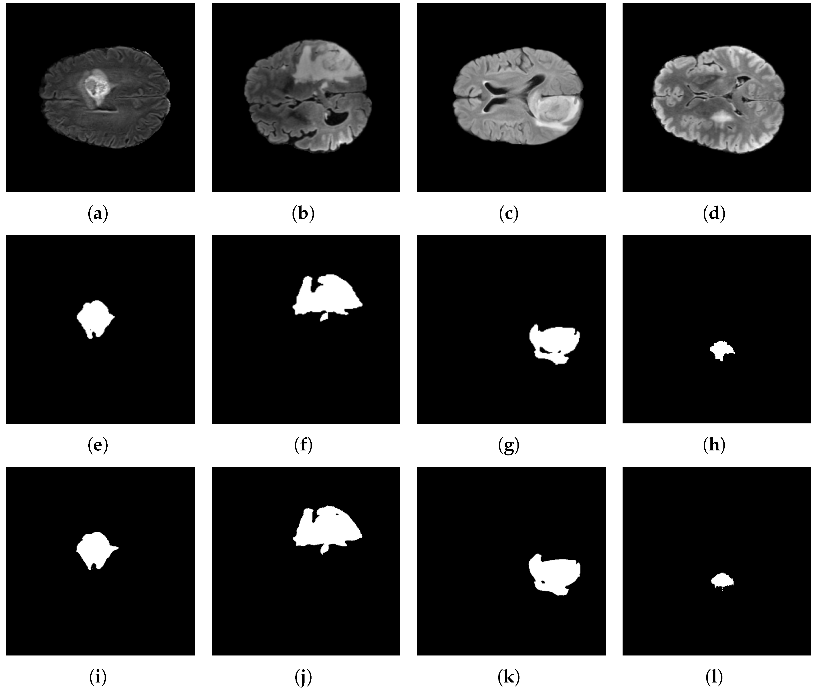
Figure 16 depicts the segmentation results for the BraTS 2023 dataset. The first row displays the original input images, the second row shows the corresponding ground-truth masks, and the third row illustrates the predictions generated by the proposed model. Figure 16e shows the ground-truth label, which exhibits an irregular morphology with a pronounced curvature; correspondingly, Figure 16i shows that the model accurately reproduces this complex boundary, yielding an essentially exact delineation.

Figure 16f depicts the ground-truth annotation of a lesion with irregular, spiculated margins; correspondingly, Figure 16j shows that the model faithfully reproduces these peak-like protrusions, preserving fine boundary detail without undue smoothing. Figure 16g depicts the ground-truth label of an irregular lesion that contains a small central region of normal-appearing tissue. Correspondingly, Figure 16k shows that the model not only recovers the overall lesion extent but also preserves this internal exclusion, refraining from labeling the central region as tumor despite its limited size. This behavior indicates precise boundary discrimination and a low propensity for over-segmentation. Furthermore, Figure 16h illustrates a comparatively small lesion. However, its limited extent poses a detection challenge; the model consistently localizes and segments the region in Figure 16l, demonstrating sensitivity to small targets.

By contrast, Figure 17 presents low-rate recognition cases in which the model’s predictions are suboptimal. Although a non-negligible portion of the lesion is correctly highlighted, relevant regions remain missed. Notably, the errors predominantly manifest as conservative under-segmentation rather than false positives, with no spurious activations in unrelated tissue. This pattern suggests a bias toward precision over recall in these instances.

Figure 18 depicts representative segmentation results on the BraTS 2024 dataset. Specifically, the first row displays the original input images, the second row shows the corresponding ground-truth masks, and the third row illustrates the predictions generated by the proposed model. Figure 18e presents a case featuring two lesions with irregular spiculated margins. The model demonstrates precise segmentation of both structures in Figure 18i, highlighting its ability to delineate multifocal tumors that accurately exhibit significant morphological heterogeneity.

Figure 18f shows the ground-truth image of a single, compact lesion with a broadly rounded contour, whereas Figure 18j presents the corresponding prediction. The model preserves the global extent and topological coherence, producing a single contiguous mask with few components and smooth, well-aligned boundaries. Figure 18g shows the ground-truth image of an irregular lesion, whereas Figure 18k presents the corresponding prediction. The model preserves location and connectivity but exhibits moderate peripheral under-segmentation, most notably along the superior–right margin, where small lobulations in the annotation are omitted, and the predicted boundary is slightly pulled inward relative to the ground-truth image.

Figure 18h shows the ground-truth image of an irregular lesion with two narrow extensions, one lateral and one inferior, connected to a compact core. Figure 18l presents the corresponding image prediction, which preserves location and topology, maintaining both extensions.

5.6. Discussion

This study demonstrates that a ConvNeXt-based multi-scale UNet augmented with a spatial latent module and Reverse Attention-guided skip connections enhances the delineation of small regions while maintaining a strong whole-tumor performance.

Table 7 presents the ablation study that highlights the quantitative contributions of the diverse architectural components, such as the optimizers, multi-scale, hybrid loss function, and Residual Attention, while evaluating the BraTS databases. First, hybridizing the BCE with a DSC loss function improved the mIoU metric and tumor delineation accuracy across BraTS 2021, 2023, and 2024, indicating that the region and contour sensitivity increased. Second, the optimizer selection adjusts the precision–recall trade-off: AdamW variants achieve higher specificity at the expense of reducing the DSC measure. In contrast, the AdamW optimizer combined with the hybrid BCE+DSC loss function provides the best overall balance, achieving higher DSC and mIoU scores and improved recovery of tiny and low-contrast tumor margins. Improved sensitivity to small enhancing regions is clinically pertinent, enabling earlier and more accurate tumor region estimation for treatment planning and progression assessment, and reducing the underestimation of active disease. Once segmentation performance is established, it may support targeted dose adjustments or earlier patient therapy modifications while reducing inter-reader variability. For clinical use, it is recommended to include site-specific threshold calibration to balance sensitivity and false positives.

TransUNet remains a strong unimodal baseline, combining ViT-driven long-range context with UNet spatial fidelity. The literature reports reliable scores when attention modules replace purely convolutional blocks [76]. In parallel, vision-language research is advancing zero-shot or few-shot transfer and automated reporting. However, segmentation still suffers from limited paired supervision, domain shift, privacy constraints, and explainability requirements, making multimodal alignment a priority for improving cross-site generalization and reducing the annotation burden [77].

6. Conclusions

Tumor segmentation was conducted on BraTS 2021, 2023, and 2024. Comparative benchmarking was reported for BraTS 2021 and 2023. However, it was not included for BraTS 2024 because no vetted segmentation studies were identified during the review period. The evaluation proceeded at the pixel level, using metrics such as IoU, DSC, sensitivity, specificity, accuracy, and F1-score. Segmentation offered greater value than classification because it produced spatially explicit contours that supported volumetry, boundary analysis, and longitudinal change assessment, thereby informing treatment planning and response evaluation. In contrast, classification provided only a global label without the spatial detail required for these downstream tasks.

The quantitative results of this study are comparable to current state-of-the-art benchmarks. Even so, the principal contribution is the effective deployment of the proposed model for pixel-wise segmentation on the BraTS datasets. Hence, image segmentation constitutes a meaningful task, clinically and methodologically more demanding and useful than per-image classification. Segmentation delivers precise localization, volumetric quantification, and subregion delineation, thereby supporting therapy planning and longitudinal monitoring; it also provides pixel-level interpretability that classification cannot offer. The findings establish a solid foundation and demonstrate the feasibility of this approach for complex medical image segmentation tasks.

7. Limitations and Future Directions

This study focused on evaluating the ConvNeXt architecture using the BraTS 2021, 2023, and 2024 datasets for brain tumor segmentation. The results capture cross-year generalization under different acquisition, preprocessing and labeling conditions. Future work considers expanding this study to external clinical datasets (e.g., TCIA-GBM and institutional MRI datasets) to increase robustness to diverse scanner types and acquisition protocols. Methodologically, the proposed neural architecture performs 2D inference using multi-scale kernels of sizes $3\times 3$, $5\times 5$, and $7\times 7$. As a result, inter-slice continuity and long-range three-dimensional dependencies are not explicitly modeled.

Moreover, the present work does not include formal calibration, volumetric uncertainty quantification, or a systematic failure-mode analysis, nor does it assess robustness to imaging artifacts or label noise. Accordingly, future work will (i) conduct external and prospective validation; (ii) incorporate volumetric context and multimodal information, including FLAIR, to improve edema-sensitive segmentation; and (iii) include subregion-specific analyses, particularly for enhancing tumor (ET) and tumor core (TC) with stratified metrics and calibration to quantify performance sensitivity across lesion phenotypes.

References

1. Ilic, I.; Ilic, M. International patterns and trends in the brain cancer incidence and mortality: An observational study based on the global burden of disease. Heliyon 2023, 9, e18222. [Google Scholar] [CrossRef]
2. Huangfu, B.; Liu, X.; Wang, X.; Niu, X.; Wang, C.; Cheng, R.; Ji, H. Global trends and burden of brain and central nervous system cancers in adolescents and young adults GBD 2021 study. Sci. Rep. 2025, 15, 17049. [Google Scholar] [CrossRef]
3. Pu, T.; Sun, J.; Ren, G.; Li, H. Neuro-immune crosstalk in cancer: Mechanisms and therapeutic implications. Signal Transduct. Target. Ther. 2025, 10, 176. [Google Scholar] [CrossRef] [PubMed]
4. Almagro, J.; Messal, H.A.; Elosegui-Artola, A.; van Rheenen, J.; Behrens, A. Tissue architecture in tumor initiation and progression. Trends Cancer 2022, 8, 494–505. [Google Scholar] [CrossRef]
5. MD Taylor, S.; Ahluwalia, M. Neoplasms of the Central Nervous System. In DeVita, Hellman, and Rosenberg’s Cancer: Principles & Practice of Oncology, 12th ed.; Wolters Kluwer: Alphen aan den Rijn, The Netherlands, 2022; Chapter 94; pp. 1568–1616. [Google Scholar]
6. Hu, A.; Razmjooy, N. Brain tumor diagnosis based on metaheuristics and deep learning. Int. J. Imaging Syst. Technol. 2021, 31, 657–669. [Google Scholar] [CrossRef]
7. Sharif, M.; Amin, J.; Raza, M.; Anjum, M.A.; Afzal, H.; Shad, S.A. Brain tumor detection based on extreme learning. Neural Comput. Appl. 2020, 32, 15975–15987. [Google Scholar] [CrossRef]
8. Satushe, V.; Vyas, V.; Metkar, S.; Singh, D.P. AI in MRI brain tumor diagnosis: A systematic review of machine learning and deep learning advances (2010–2025). Chemom. Intell. Lab. Syst. 2025, 263, 105414. [Google Scholar] [CrossRef]
9. National Cancer Institute and SEER (Surveillance-Epidemiology and End-Results Program). Brain and Other Nervous System Cancer—Cancer Stat Facts. 2024. Available online: https://seer.cancer.gov/statfacts/html/brain.html (accessed on 14 August 2025).
10. World Health Organization. WHO Mortality Database. 2024. Available online: https://platform.who.int/mortality/themes/theme-details/topics/indicator-groups/indicator-group-details/MDB/brain-and-nervous-system-cancers (accessed on 14 August 2025).
11. Filho, A.M.; Znaor, A.; Sunguc, C.; Zahwe, M.; Marcos-Gragera, R.; Figueroa, J.D.; Bray, F. Cancers of the brain and central nervous system: Global patterns and trends in incidence. J. Neurooncol. 2025, 172, 567–578. [Google Scholar] [CrossRef] [PubMed]
12. Ferlay, J.; Laversanne, M.; Ervik, M.; Lam, F.; Colombet, M.; Mery, L.; Piñeros, M.; Znaor, A.; Soerjomataram, I. Global Cancer Observatory: Cancer Tomorrow, International Agency for Research on Cancer. Available online: https://gco.iarc.who.int/tomorrow (accessed on 28 May 2025).
13. Batool, A.; Byun, Y.C. Brain tumor detection with integrating traditional and computational intelligence approaches across diverse imaging modalities - Challenges and future directions. Comput. Biol. Med. 2024, 175, 108412. [Google Scholar] [CrossRef]
14. Arora, V.; Sidhu, B.S.; Singh, K. Comparison of computed tomography and magnetic resonance imaging in evaluation of skull lesions. Egypt. J. Radiol. Nucl. Med. 2022, 53, 67. [Google Scholar] [CrossRef]
15. de Marco, G.; Peretti, I. Magnetic Resonance Imaging: Basic Principles and Applications. In The Neuroimaging of Brain Diseases: Structural and Functional Advances; Habas, C., Ed.; Springer International Publishing: Cham, Switzerland, 2018; pp. 1–25. [Google Scholar] [CrossRef]
16. Bonato, B.; Nanni, L.; Bertoldo, A. Advancing Precision: A Comprehensive Review of MRI Segmentation Datasets from BraTS Challenges (2012–2025). Sensors 2025, 25, 1838. [Google Scholar] [CrossRef]
17. Kwok, W.E. Radiofrequency interference in magnetic resonance imaging: Identification and rectification. J. Clin. Imaging Sci. 2024, 14, 33. [Google Scholar] [CrossRef]
18. Ortega-Robles, E.; de Celis Alonso, B.; Cantillo-Negrete, J.; Carino-Escobar, R.I.; Arias-Carrión, O. Advanced Magnetic Resonance Imaging for Early Diagnosis and Monitoring of Movement Disorders. Brain Sci. 2025, 15, 79. [Google Scholar] [CrossRef] [PubMed]
19. Saad, N.S.; Gad, A.A.; Elzoghby, M.M.; Ibrahim, H.R. Comparison between the diagnostic utility of three-dimensional fluid attenuated inversion recovery (3D FLAIR) and three dimensional double inversion recovery (3D DIR) magnetic resonance sequences in the assessment of overall load of multiple sclerosis lesions in the brain. Egypt. J. Radiol. Nucl. Med. 2024, 55, 156. [Google Scholar] [CrossRef]
20. Wilson, H.; de Natale, E.R.; Politis, M. Chapter 2—Advances in magnetic resonance imaging. In Neuroimaging in Parkinson’s Disease and Related Disorders; Politis, M., Wilson, H., De Natale, E.R., Eds.; Academic Press: Cambridge, MA, USA, 2023; pp. 21–52. [Google Scholar] [CrossRef]
21. Lu, Z.; Yan, J.; Zeng, J.; Zhang, R.; Xu, M.; Liu, J.; Sun, L.; Zu, G.; Chen, X.; Zhang, Y.; et al. Time-resolved T1 and T2 contrast for enhanced accuracy in MRI tumor detection. Biomaterials 2025, 321, 123313. [Google Scholar] [CrossRef] [PubMed]
22. Bailey, W.M. Fast Fluid Attenuated Inversion Recovery (FLAIR) imaging and associated artefacts in Magnetic Resonance Imaging (MRI). Radiography 2007, 13, 283–290. [Google Scholar] [CrossRef]
23. Abdusalomov, A.B.; Mukhiddinov, M.; Whangbo, T.K. Brain Tumor Detection Based on Deep Learning Approaches and Magnetic Resonance Imaging. Cancers 2023, 15, 4172. [Google Scholar] [CrossRef]
24. Rayed, M.E.; Islam, S.S.; Niha, S.I.; Jim, J.R.; Kabir, M.M.; Mridha, M. Deep learning for medical image segmentation: State-of-the-art advancements and challenges. Inform. Med. Unlocked 2024, 47, 101504. [Google Scholar] [CrossRef]
25. Kaur, R.; Singh, S. A comprehensive review of object detection with deep learning. Digit. Signal Process. 2023, 132, 103812. [Google Scholar] [CrossRef]
26. Huda, N.; Ku-Mahamud, K.R. CNN-Based Image Segmentation Approach in Brain Tumor Classification: A Review. Eng. Proc. 2025, 84, 66. [Google Scholar] [CrossRef]
27. Takahashi, S.; Sakaguchi, Y.; Kouno, N.; Takasawa, K.; Ishizu, K.; Akagi, Y.; Aoyama, R.; Teraya, N.; Bolatkan, A.; Shinkai, N.; et al. Comparison of Vision Transformers and Convolutional Neural Networks in Medical Image Analysis: A Systematic Review. J. Med. Syst. 2024, 48, 84. [Google Scholar] [CrossRef]
28. He, K.; Gan, C.; Li, Z.; Rekik, I.; Yin, Z.; Ji, W.; Gao, Y.; Wang, Q.; Zhang, J.; Shen, D. Transformers in medical image analysis. Intell. Med. 2023, 3, 59–78. [Google Scholar] [CrossRef]
29. Kotyan, S.; Vargas, D.V. Improving robustness for vision transformer with a simple dynamic scanning augmentation. Neurocomputing 2024, 565, 127000. [Google Scholar] [CrossRef]
30. Synapse Platform. BraTS 2021 Data Description. Available online: https://www.synapse.org/Synapse:syn25829067/wiki/610863 (accessed on 6 December 2024).
31. Synapse Platform. BraTS 2023 Data Description. Available online: https://www.synapse.org/Synapse:syn51156910/wiki/621282 (accessed on 6 December 2024).
32. Synapse Platform. BraTS 2024 Data Description. Available online: https://www.synapse.org/Synapse:syn53708249/wiki/626323 (accessed on 6 December 2024).
33. Andrade-Miranda, G.; Jaouen, V.; Bourbonne, V.; Lucia, F.; Visvikis, D.; Conze, P.H. Pure Versus Hybrid Transformers For Multi-Modal Brain Tumor Segmentation: A Comparative Study. In Proceedings of the 2022 IEEE International Conference on Image Processing (ICIP), Bordeaux, France, 16–19 October 2022; pp. 1336–1340. [Google Scholar] [CrossRef]
34. Elharrouss, O.; Akbari, Y.; Almadeed, N.; Al-Maadeed, S. Backbones-review: Feature extractor networks for deep learning and deep reinforcement learning approaches in computer vision. Comput. Sci. Rev. 2024, 53, 100645. [Google Scholar] [CrossRef]
35. Yang, H.; Shen, Z.; Li, Z.; Liu, J.; Xiao, J. Combining Global Information with Topological Prior for Brain Tumor Segmentation. In Brainlesion: Glioma, Multiple Sclerosis, Stroke and Traumatic Brain Injuries; Crimi, A., Bakas, S., Eds.; Springer: Cham, Switzerland, 2022; pp. 204–215. [Google Scholar] [CrossRef]
36. Chen, X.; Yang, L. Brain tumor segmentation based on CBAM-TransUNet. In Proceedings of the 1st ACM Workshop on Mobile and Wireless Sensing for Smart Healthcare (MWSSH ‘22), New York, NY, USA, 12 April 2022; pp. 33–38. [Google Scholar] [CrossRef]
37. Jia, Q.; Shu, H. BiTr-Unet: A CNN-Transformer Combined Network for MRI Brain Tumor Segmentation. In Brainlesion: Glioma, Multiple Sclerosis, Stroke and Traumatic Brain Injuries; Crimi, A., Bakas, S., Eds.; Springer: Cham, Switzerland, 2022; pp. 3–14. [Google Scholar] [CrossRef]
38. Jiang, Y.; Zhang, Y.; Lin, X.; Dong, J.; Cheng, T.; Liang, J. SwinBTS: A Method for 3D Multimodal Brain Tumor Segmentation Using Swin Transformer. Brain Sci. 2022, 12, 797. [Google Scholar] [CrossRef]
39. ZongRen, L.; Silamu, W.; Yuzhen, W.; Zhe, W. DenseTrans: Multimodal Brain Tumor Segmentation Using Swin Transformer. IEEE Access 2023, 11, 42895–42908. [Google Scholar] [CrossRef]
40. Praveen, M.; Evuri, N.; Pakala, S.R.; Samantula, S.; Chebrolu, S. 3D Swin-Res-SegNet: A Hybrid Transformer and CNN Model for Brain Tumor Segmentation Using MRI Scans. J. Inst. Eng. (India) Ser. B 2025, 106, 1489–1499. [Google Scholar] [CrossRef]
41. Lin, J.; Lin, J.; Lu, C.; Chen, H.; Lin, H.; Zhao, B.; Shi, Z.; Qiu, B.; Pan, X.; Xu, Z.; et al. CKD-TransBTS: Clinical Knowledge-Driven Hybrid Transformer With Modality-Correlated Cross-Attention for Brain Tumor Segmentation. IEEE Trans. Med. Imaging 2023, 42, 2451–2461. [Google Scholar] [CrossRef]
42. Dobko, M.; Kolinko, D.I.; Viniavskyi, O.; Yelisieiev, Y. Combining CNNs with Transformer for Multimodal 3D MRI Brain Tumor Segmentation. In Brainlesion: Glioma, Multiple Sclerosis, Stroke and Traumatic Brain Injuries; Crimi, A., Bakas, S., Eds.; Springer: Cham, Switzerland, 2022; pp. 232–241. [Google Scholar] [CrossRef]
43. Bhagyalaxmi, K.; Dwarakanath, B. CDCG-UNet: Chaotic Optimization Assisted Brain Tumor Segmentation Based on Dilated Channel Gate Attention U-Net Model. Neuroinformatics 2025, 23, 12. [Google Scholar] [CrossRef]
44. Wu, Y.; Li, Q. ConvNeXt embedded U-Net for semantic segmentation in urban scenes of multi-scale targets. Complex Intell. Syst. 2025, 11, 181. [Google Scholar] [CrossRef]
45. Deng, S.; Yang, Y.; Wang, J.; Li, A.; Li, Z. Efficient SpineUNetX for X-ray: A spine segmentation network based on ConvNeXt and UNet. J. Vis. Commun. Image Represent. 2024, 103, 104245. [Google Scholar] [CrossRef]
46. Mallick, S.; Paul, J.; Sil, J. Response Fusion Attention U-ConvNext for accurate segmentation of optic disc and optic cup. Neurocomputing 2023, 559, 126798. [Google Scholar] [CrossRef]
47. Zhang, H.; Zhong, X.; Li, G.; Liu, W.; Liu, J.; Ji, D.; Li, X.; Wu, J. BCU-Net: Bridging ConvNeXt and U-Net for medical image segmentation. Comput. Biol. Med. 2023, 159, 106960. [Google Scholar] [CrossRef] [PubMed]
48. Chen, J.; Wang, R.; Dong, W.; He, H.; Wang, S. HistoNeXt: Dual-mechanism feature pyramid network for cell nuclear segmentation and classification. BMC Med. Imaging 2025, 25, 9. [Google Scholar] [CrossRef] [PubMed]
49. Hu, Z.; Wang, Y.; Xiao, L. Alzheimer’s disease diagnosis by 3D-SEConvNeXt. J. Big Data 2025, 12, 15. [Google Scholar] [CrossRef]
50. Madhavi, B.; Mahanty, M.; Lin, C.C.; Lakshmi Jagan, B.O.; Rai, H.M.; Agarwal, S.; Agarwal, N. SwinConvNeXt: A fused deep learning architecture for Real-time garbage image classification. Sci. Rep. 2025, 15, 7995. [Google Scholar] [CrossRef] [PubMed]
51. Han, G. Bio-inspired swarm intelligence for enhanced real-time aerial tracking: Integrating whale optimization and grey wolf optimizer algorithms. Discov. Artif. Intell. 2025, 5, 18. [Google Scholar] [CrossRef]
52. Asif, S.; Raza Shahid, A.; Aftab, K.; Ather Enam, S. Integrating the Prior Shape Knowledge Into Deep Model and Feature Fusion for Topologically Effective Brain Tumor Segmentation. IEEE Access 2025, 13, 99641–99658. [Google Scholar] [CrossRef]
53. Encío, L.; Díaz, C.; del Blanco, C.R.; Jaureguizar, F.; García, N. Visual Parking Occupancy Detection Using Extended Contextual Image Information via a Multi-Branch Output ConvNeXt Network. Sensors 2023, 23, 3329. [Google Scholar] [CrossRef]
54. Huang, J.; Wu, Y.; Zhuang, M.; Zhou, J. High-Precision and Efficiency Hardware Implementation for GELU via Its Internal Symmetry. Electronics 2025, 14, 1825. [Google Scholar] [CrossRef]
55. Lee, M. Mathematical Analysis and Performance Evaluation of the GELU Activation Function in Deep Learning. J. Math. 2023, 2023, 4229924. [Google Scholar] [CrossRef]
56. Liu, T.; Zhang, P.; Huang, W.; Zha, Y.; You, T.; Zhang, Y. How does Layer Normalization improve Batch Normalization in self-supervised sound source localization? Neurocomputing 2024, 567, 127040. [Google Scholar] [CrossRef]
57. Bishop, C.M.; Bishop, H. Gradient Descent. In Deep Learning: Foundations and Concepts; Springer International Publishing: Cham, Switzerland, 2024; pp. 209–232. [Google Scholar] [CrossRef]
58. Nguyen, K.B.; Choi, J.; Yang, J.S. EUNNet: Efficient UN-Normalized Convolution Layer for Stable Training of Deep Residual Networks without Batch Normalization Layer. IEEE Access 2023, 11, 76977–76988. [Google Scholar] [CrossRef]
59. Tolic, A.; Mileva Boshkoska, B.; Skansi, S. Chrono Initialized LSTM Networks with Layer Normalization. IEEE Access 2024, 12, 115219–115236. [Google Scholar] [CrossRef]
60. Ye, J.C. Normalization and Attention. In Geometry of Deep Learning: A Signal Processing Perspective; Springer Nature: Singapore, 2022; pp. 155–191. [Google Scholar] [CrossRef]
61. Niu, Z.; Deng, Z.; Gao, W.; Bai, S.; Gong, Z.; Chen, C.; Rong, F.; Li, F.; Ma, L. FNeXter: A Multi-Scale Feature Fusion Network Based on ConvNeXt and Transformer for Retinal OCT Fluid Segmentation. Sensors 2024, 24, 2425. [Google Scholar] [CrossRef] [PubMed]
62. Y., N.; Gopal, J. An automatic classification of breast cancer using fuzzy scoring based ResNet CNN model. Sci. Rep. 2025, 15, 20739. [Google Scholar] [CrossRef]
63. Wang, Z.; Xie, X.; Yang, J.; Song, X. RA-Net: Reverse attention for generalizing residual learning. Sci. Rep. 2024, 14, 12771. [Google Scholar] [CrossRef]
64. Lee, G.E.; Cho, J.; Choi, S.I. Shallow and reverse attention network for colon polyp segmentation. Sci. Rep. 2023, 13, 15243. [Google Scholar] [CrossRef]
65. Xu, W.; Fu, Y.L.; Zhu, D. ResNet and its application to medical image processing: Research progress and challenges. Comput. Methods Programs Biomed. 2023, 240, 107660. [Google Scholar] [CrossRef]
66. Liu, Z.; Mao, H.; Wu, C.Y.; Feichtenhofer, C.; Darrell, T.; Xie, S. A ConvNet for the 2020s. In Proceedings of the 2022 IEEE/CVF Conference on Computer Vision and Pattern Recognition (CVPR), New Orleans, LA, USA, 18–24 June 2022; pp. 11966–11976. [Google Scholar] [CrossRef]
67. Zhou, P.; Xie, X.; Lin, Z.; Yan, S. Towards Understanding Convergence and Generalization of AdamW. IEEE Trans. Pattern Anal. Mach. Intell. 2024, 46, 6486–6493. [Google Scholar] [CrossRef]
68. Kato, S.; Hotta, K. Adaptive t-vMF dice loss: An effective expansion of dice loss for medical image segmentation. Comput. Biol. Med. 2024, 168, 107695. [Google Scholar] [CrossRef]
69. Ma, J.; He, Y.; Li, F.; Han, L.; You, C.; Wang, B. Segment anything in medical images. Nat. Commun. 2024, 15, 654. [Google Scholar] [CrossRef] [PubMed]
70. Fan, Y.; Hu, Z.; Li, Q.; Sun, Y.; Chen, J.; Zhou, Q. CrackNet: A Hybrid Model for Crack Segmentation with Dynamic Loss Function. Sensors 2024, 24, 7134. [Google Scholar] [CrossRef]
71. Lv, P.; Xu, H.; Zhang, Q.; Shi, L.; Li, H.; Chen, Y.; Zhang, Y.; Cao, D.; Liu, Z.; Liu, Y.; et al. An improved lightweight ConvNeXt for rice classification. Alex. Eng. J. 2025, 112, 84–97. [Google Scholar] [CrossRef]
72. Kordnoori, S.; Sabeti, M.; Mostafaei, H.; Seyed Agha Banihashemi, S. Advances in medical image analysis: A comprehensive survey of lung infection detection. IET Image Process. 2024, 18, 3750–3800. [Google Scholar] [CrossRef]
73. Rizwan I Haque, I.; Neubert, J. Deep learning approaches to biomedical image segmentation. Inform. Med. Unlocked 2020, 18, 100297. [Google Scholar] [CrossRef]
74. Hicks, S.A.; Strümke, I.; Thambawita, V.; Hammou, M.; Riegler, M.A.; Halvorsen, P.; Parasa, S. On evaluation metrics for medical applications of artificial intelligence. Sci. Rep. 2022, 12, 5979. [Google Scholar] [CrossRef] [PubMed]
75. Nguyen-Tat, T.B.; Nguyen, T.Q.T.; Nguyen, H.N.; Ngo, V.M. Enhancing brain tumor segmentation in MRI images: A hybrid approach using UNet, attention mechanisms, and transformers. Egypt. Inform. J. 2024, 27, 100528. [Google Scholar] [CrossRef]
76. Li, X.; Li, L.; Jiang, Y.; Wang, H.; Qiao, X.; Feng, T.; Luo, H.; Zhao, Y. Vision-Language Models in medical image analysis: From simple fusion to general large models. Inf. Fusion 2025, 118, 102995. [Google Scholar] [CrossRef]
77. Li, X.; Sun, Y.; Lin, J.; Li, L.; Feng, T.; Yin, S. The Synergy of Seeing and Saying: Revolutionary Advances in Multi-modality Medical Vision-Language Large Models. Artif. Intell. Sci. Eng. 2025, 1, 79–97. [Google Scholar] [CrossRef]
Figure 1. Estimated global mortality rate attributable to brain tumors. Chart generated by the authors from data available at the International Agency for Research on Cancer (IARC) website (https://gco.iarc.who.int/tomorrow/en, accessed on 13 December 2025), the Global Cancer Observatory: Cancer Tomorrow database [12].
Technologies 14 00034 g001
Figure 2. Comparative axial slices from the BraTS 2023 dataset showing (a) native T1-weighted (T1), (b) contrast-enhanced T1-weighted (T1-C), and (c) T2-weighted (T2) MRI sequences, together with (d) the corresponding ground-truth tumor mask.
Technologies 14 00034 g002
Figure 3. Architectural overview of the Vision Transformer (ViT-Base) model, highlighting patch tokenization, positional encoding, stacked Transformer encoder layers, and the classification head.
Technologies 14 00034 g003
Figure 4. Sampling configurations: (a) Partial overlapping (stride smaller than filter size), and (b) non-overlapping (stride equals filter size). Original image pixels in light-blue, sliding window in the ( k ) t h -, ( k + 1 ) t h -, and ( k + 2 ) t h -iterations colored in green, blue, and yellow, respectively.
Technologies 14 00034 g004
Figure 5. Comparison of the Gaussian error linear unit (GELU) and the rectified linear unit (ReLU) activation functions. While ReLU enforces a hard zero-threshold, GELU introduces a smooth, probabilistic transition that better preserves negative values near the origin.
Technologies 14 00034 g005
Figure 6. Comparative overview of feature-wise normalization techniques: (a) Batch normalization (BN); statistics computed across the mini-batch for each feature channel; (b) layer normalization (LN); statistics computed across all features for each sample. The green color indicates the voxels to be analyzed, and the process continues with the adjacent yellow voxels.
Technologies 14 00034 g006
Figure 7. Multi-scale feature extraction: The input image passes through three convolutional branches of size 3 × 3 , 5 × 5 , and 7 × 7 . In addition, the feature maps are stacked into a fused feature map.
Technologies 14 00034 g007
Figure 8. Reverse Attention (RA) module [64], where F k and F k + 1 are the feature maps at stages k and k + 1 , s ( · ) denotes the sigmoid function, ⊗ represents element-wise multiplication (Hadamard product), and F k R A is the RA-refined feature map.
Technologies 14 00034 g008
Figure 9. Visual comparison of a ResNet-style residual bottleneck and an inverted bottleneck: (a) Residual bottleneck; (b) inverted bottleneck.
Technologies 14 00034 g009
Figure 10. Three-dimensional visualization of a BraTS T1-MRI volumetric image, showing the spatial distribution of anatomical structures across all slices.
Technologies 14 00034 g010
Figure 11. A single voxel in the mask image comprises multiple slices, particularly those including sensitive information to (a) identify the slice containing the highest proportion of mask content. (b) 3D scatter visualization of the ground-truth mask.
Technologies 14 00034 g011
Figure 12. Comparison of computational resource usage in Swin Transformer, ResNet, and ConvNeXt neural blocks. (a) Swin Transformer block; (b) ResNet block; (c) ConvNeXt block.
Technologies 14 00034 g012
Figure 13. Architecture of the proposed model, comprising a modified UNet with a ConvNeXt backbone, preceded by a multi-scale feature extraction module, and further enhanced with an RA module.
Technologies 14 00034 g013
Figure 14. Box plots of DSC, IoU, sensitivity, specificity, accuracy, and F1-score under 5-fold cross-validation for BraTS 2021, 2023, and 2024. Boxes depict the interquartile range with the median; whiskers indicate the range of non-outlier data per software defaults; and outliers are shown as individual points. Overlaid 95% confidence intervals summarize uncertainty across folds. (a) BraTS 2021; (b) BraTS 2023; (c) BraTS 2024. Hollow circles are the outliers >   1.5 × IQR from the box and red dot is the arithmetic mean.
Technologies 14 00034 g014
Figure 15. Brain tumor segmentation results using the BraTS 2021 dataset and the proposed architecture. Original images: (ad); target images: (eh); and predicted images: (il).
Technologies 14 00034 g015
Figure 16. Brain tumor segmentation using the BraTS 2023 dataset and the proposed architecture. Original images: (ad); target images: (eh); and predicted images: (il).
Technologies 14 00034 g016
Figure 17. Exceptional cases where the model behaved poorly with the BraTS 2023 dataset with the proposed architecture. Original images: (a,d); target images: (b,e); and predicted images: (c,f).
Technologies 14 00034 g017
Figure 18. Brain tumor segmentation using the BraTS 2024 dataset and the proposed architecture. Original images: (ad); target images: (eh); and predicted images: (il).
Technologies 14 00034 g018