Dynamic Updating of Geological Models by Directly Interpolating Geological Logging Data

Abstract

Traditional orebody modeling methods struggle to efficiently integrate new geological data. Therefore, we propose a novel framework for dynamically updating 3D geological models by directly interpolating geological logging data. The core innovation lies in the innovative interpolation of raw interpreted cross polylines into an implicit scalar field representation without intermediate explicit surface extraction or manual remodeling. To obtain reliable vectorized polylines, we developed image recognition and digitization techniques that are based on the pattern recognition of geological sketches. Moreover, different from existing implicit techniques, we present an improved approach to interpolate complex cross polylines that are dynamically based on the improved principal component analysis. The method allows specifying a priori constraints to adjust the erroneous estimated normal to improve the reliability of the normal estimation results of cross-contour polylines. The a priori information can be combined into the normal estimation algorithm to update the normals of the corresponding adjacent contour polylines in the process of normal estimation at the intersection points and in the process of normal propagation. By leveraging the radial basis functions-based spatial interpolators, the method continuously assimilates incremental geological observations into the interpolation constraints to update the implicit model. Case studies demonstrate a reduction in the modeling cycle time compared to conventional explicit methods while maintaining geologically coherent boundaries. The framework significantly enhances decision agility in resource estimation and mine planning workflows by bridging geological interpretation and dynamic model iteration.

1. Introduction

Geological implicit modeling is pivotal for constructing three-dimensional (3D) models of geological bodies by using sparse sampling data, thus enabling the integration and interpretation of multi-source heterogeneous geological data. A key challenge in this domain is the dynamic reconstruction of accurate 3D orebody models from complex cross-contour polylines, particularly when updating models with new geological data. Traditional explicit modeling methods, with their low automation and inability to dynamically update, fail to meet the demands of rapid resource estimation and real-time model adjustments during production exploration.

Cross-contour polylines in mine production mostly originate from geological logging. Mine geological logging is a critical process in operational mining, involving systematic documentation of geological phenomena in exploration boreholes, development headings, and production drifts through textual descriptions, standardized charts, and sketch maps. These records provide high-fidelity spatially referenced data that are essential for delineating orebody morphology and ore-rock boundaries, thus supporting mine planning and resource estimation. Integral to orebody model updating workflows, the raw geological sketches and maps generated from geological logging should be further processed. To obtain reliable vectorized polylines, we developed image recognition and digitization techniques based on the pattern recognition of geological sketches. This facilitates the extraction of geologically interpreted polylines that represent local geometry features. These interpreted polylines are then rigorously utilized to update and refine the orebody model, thereby ensuring its ongoing accuracy and reliability for mine planning, reserve estimation, and operational decision-making throughout the mine lifecycle.

Recent advancements in artificial intelligence (AI) and machine learning (ML) [1,2,3,4] have significantly advanced geological data digitalization and model updating. For example, Zhang et al. [1] introduced an AI-based framework for the automated extraction of geological features from borehole data, thus improving model updating efficiency by 30% over manual methods. Similarly, Rotem et al. [2] applied a convolutional neural network (CNN)-based approach to interpret hyperspectral shortwave infrared core scanning data, automating mineral identification and improving geological model accuracy in mineral exploration. Additionally, Lyu et al. [3] developed a multi-scale generative adversarial network (GAN) for generating 3D subsurface geological models from limited borehole data, achieving improved resolution and geological consistency by integrating prior geological knowledge. These studies underscore the potential of AI/ML to improve automation in implicit modeling, particularly for dynamic 3D model updates. However, up to now, they are still not competent enough for the task of dynamic orebody modeling that is based on complex cross-contour polylines.

It is an important and difficult problem in the research of digital mines to model geological bodies that are based on a large number of complex cross-contour polylines. Currently, there are several approaches for contour modeling. A common practice is to triangulate the contour polylines using the Delaunay triangulation methods [5,6,7,8]. Another common practice is to represent the geometry model using the way of free-form curves and surfaces [9,10]. The most commonly used surface-fitting methods include the Bezier method [11], the B-spline method [12,13], and the Nurbs method [14]. However, the above two types of approaches make it difficult to process the contour polylines with complex topology relationships. The most promising approach is to interpolate the contour polylines using implicit modeling methods [15,16,17]. This type of method interpolates the contours using an implicit function (e.g., the radial basis function [18]) and extracts the isosurface using a surface reconstruction method (e.g., the marching cubes [19,20] and the marching tetrahedra methods [21,22]). It is certain that there are some other modeling methods [23], including methods [24,25,26] that combine the above several approaches by using some new ideas.

In this paper, we mainly focus on the third approach, namely the contour interpolation method. At present, most of the existing studies [27,28] of contour interpolation are suitable for the cases in which each contour polyline is coplanar. For the non-coplanar polylines, a very important problem for contour interpolation or contour modeling is to determine the orientation of the contour polylines or the topological relationship between the contour polylines. Though there are some works [29,30] on contour modeling that do not calculate the normal orientations of contour polylines, these methods require determining the interior and exterior position relationships or other prior input polyline information by using specific ways (e.g., geometry sampling). Generally, the implicit modeling method needs to convert the original geological sampling data and manually interpreted data into interpolation constraints. The automation of this method still mainly depends on the automatic construction of interpolation constraints. However, there is no robust method to automatically determine the normal direction of multiple sparse and uneven contours.

Our work specifically addresses the critical challenge of reconstructing accurate and geologically plausible 3D orebody models from specific geological data, with a primary focus on cross polylines. To model the orebody, based on the geological interpreted data of complex cross-contour polylines, we transformed the original contour polylines into oriented polylines and utilized the implicit modeling method to reconstruct the orebody model dynamically. To improve the reliability of the normal estimation results of contour polylines, we propose a normal estimation method of contour polylines that allows a manual adjustment of some normals based on the combination of the point cloud normal dynamic estimation [31] and cross-contour normal estimation methods [32]. Generally speaking, the normal estimation method of contour polylines contains two basic strategies as follows: the approximate estimation rule at intersections, and the manual a priori rule. The approximate estimation rule at intersections is based on the assumption that the local geometric features of the contour polylines near the intersection point satisfy the condition of the least squares fitting plane. However, if the normal estimation at the intersection point is erroneous, the normal reorientation of the adjacent polylines at the corresponding intersection point may fail, which will affect the normal propagation process. In this case, the manual a priori rule can be used to adjust the erroneous estimated normal to improve the reliability of the normal estimation results of cross-contour polylines.

On the basis of transforming the problem of contour normal estimation into a problem of normal estimation of the point cloud at the intersection points, an implicit modeling method of orebody that can dynamically estimate the normals of cross-contour polylines is proposed in this paper. The method allows geological engineers to interactively adjust the normals of some contour polylines according to the geological rules, and thus, automatically update the normals of the corresponding adjacent contour polylines in the process of normal estimation at the intersection points and in the process of normal propagation.

2. Method Overview

2.1. Method

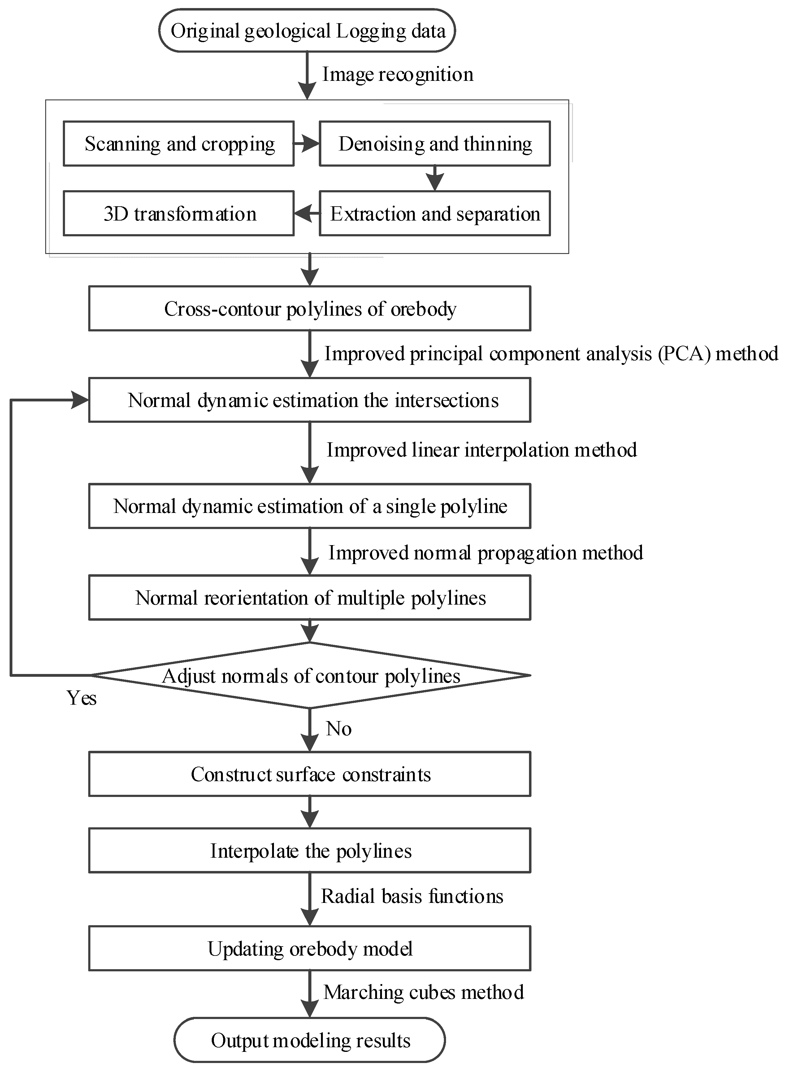
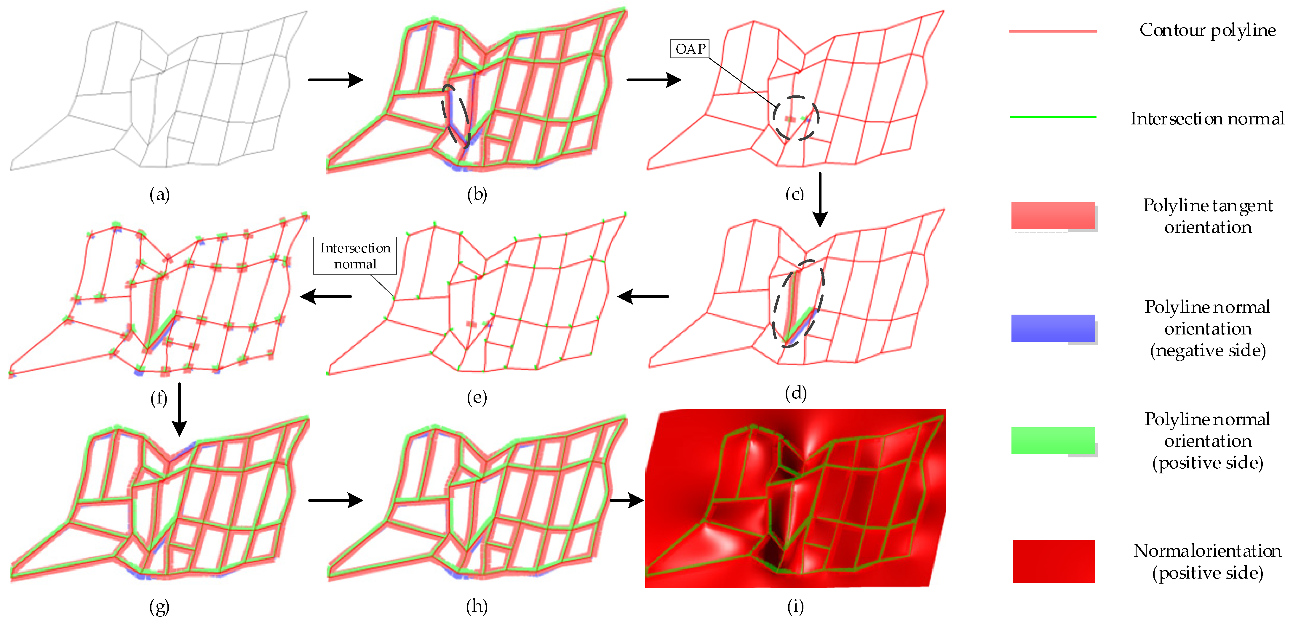
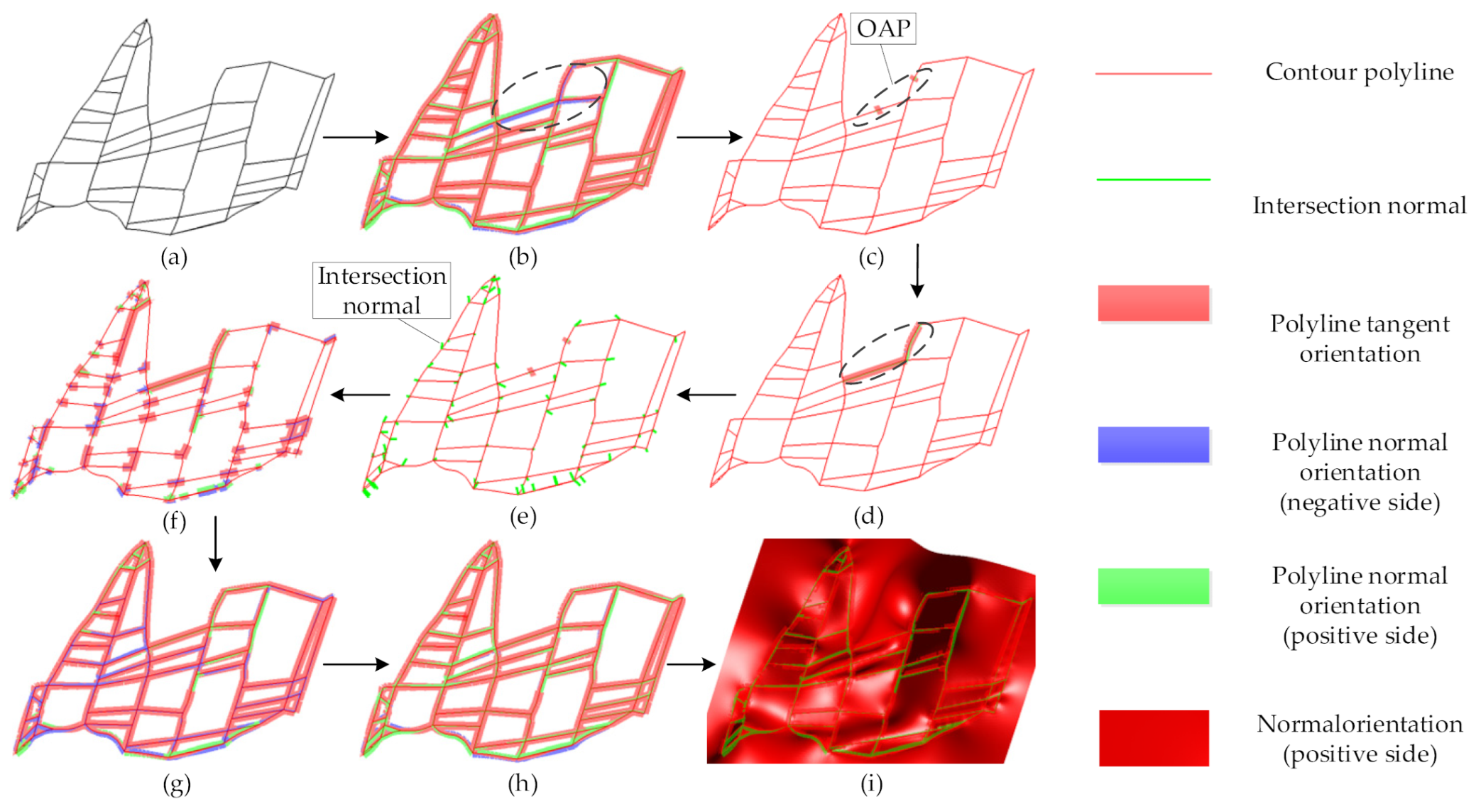
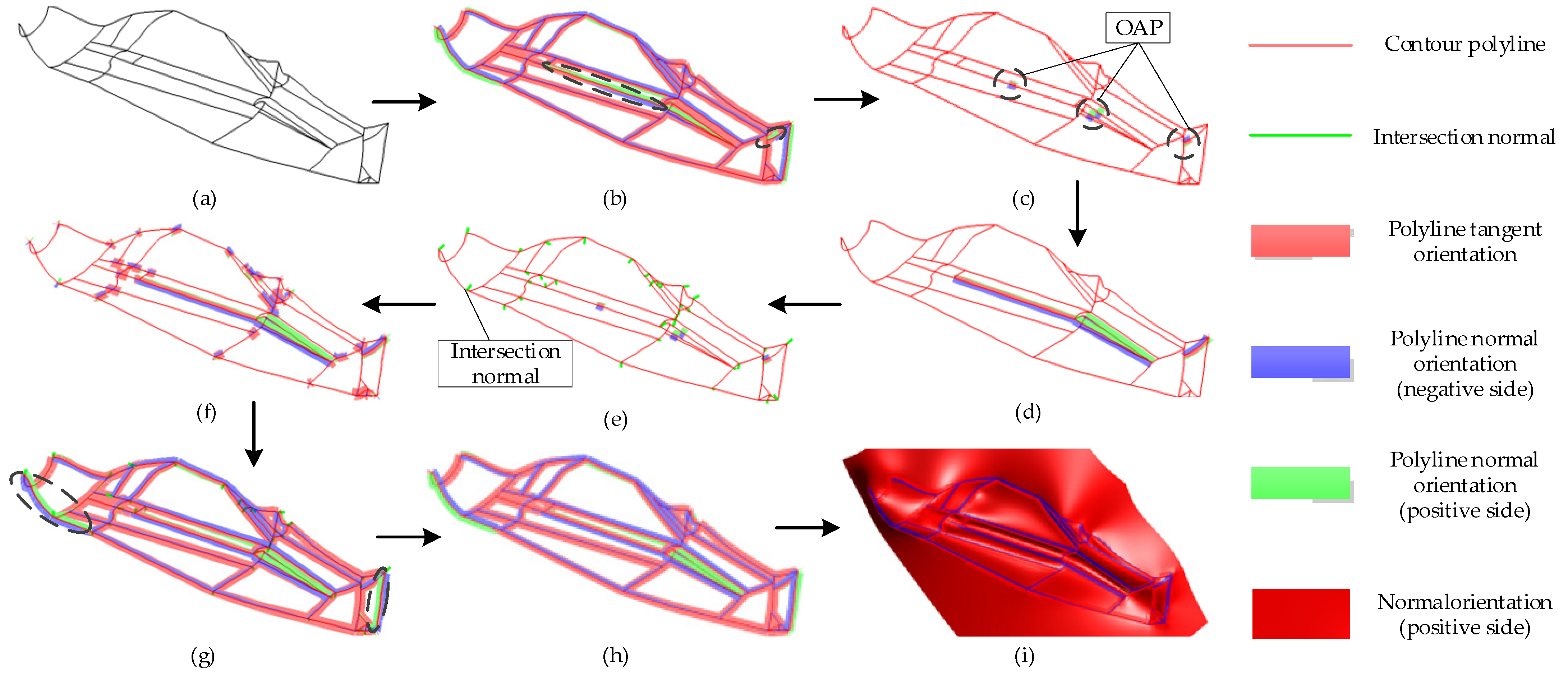
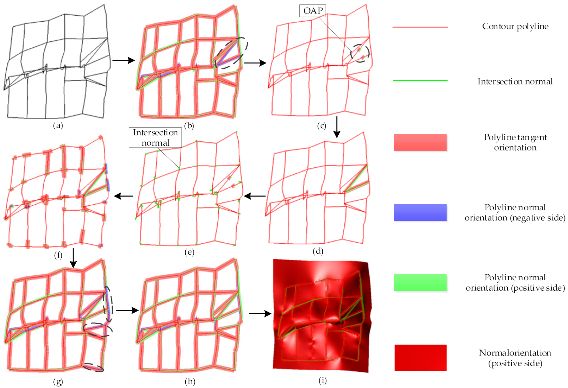
The overall goal is to reconstruct and dynamically update 3D implicit orebody models directly from geological logging data. The method proposed in this paper consists of the following steps.

(1)

Scan regions from the original geological log drawings and then crop the relevant graphical sections.

(2)

Convert the cropped image to grayscale and perform noise removal.

(3)

Trace the connected non-zero pixels to extract the boundary polylines.

(4)

Transform the vectorized 2D boundaries to true 3D positions via translation, scaling, rotation, and projection.

(5)

Preprocess the data of the geological interpreted contour polylines.

(6)

Interpolate the normals of the intersections of cross-contour polylines.

(7)

Estimate the normals of a single contour polyline.

(8)

Reorient the normals of multiple contour polylines.

(9)

Adjust the normals of some segments according to the a priori geological rule and re-estimate the normals of the contour polylines.

(10)

Convert the directional polylines into surface constraints.

(11)

Interpolate the polylines using radial basis functions.

(12)

Update the orebody model using the marching cubes method.

The overall flow chart of the method is shown in Figure 1.

2.2. Terminology

Cross-Contour Polylines: These are 2D or 3D line segments that are derived from geological sketches and represent the intersections of geological surfaces with sampling planes and are used to reconstruct 3D orebody models.

Normal Vector: This is a unit vector that is perpendicular to an intersection or a polyline segment and is used to define the orientation for interpolation.

Network Graph: This is a graph structure with nodes as intersection points of the polylines and edges as the polyline segments, thus capturing the topological relationships.

Neighborhood Points: These are points within a specified radius around an intersection and are used for normal estimation.

Oriented/Unoriented Neighborhood Points (ONP/UNP): These are points with or without predefined normal vectors, and they are used to distinguish between user-specified and algorithmically estimated normals.

Oriented/Unoriented Adjacent Polylines (OAP/UAP): These are polylines that are adjacent to the intersection with or without predefined normal vectors, and these are used to distinguish between the user-specified and algorithmically estimated normals.

Normal Reorientation Rule: This method employs a strict confidence ranking to define the normal reorientation rule: User-predefined normals (based on prior geological knowledge) > propagated normals (derived from high-confidence anchors via BFS) > PCA-estimated normals (based on local geometric fitting).

3. Geological Implicit Modeling

The basic processes of implicit modeling can be summarized as follows. Following the implicit function field modeling approach, discretely sampled geological data are first converted into spatial interpolation constraints. An implicit function characterizing the spatial potential field distribution of mineralization is then determined through the spatial interpolation methods that are governed by specific geological rules. The surface model of the orebody is represented as a specific isosurface of this implicit function (e.g., the zero-isosurface $f\left(\mathit{x}\right)=0$). To reconstruct the continuous implicit function representing the orebody model, discrete sampling of mineralized space can be performed, with the function values at the sampling points being evaluated through the implicit function to recover the target isosurface. During any stage of orebody modeling, sampling data and geological constraints can be added, modified, or updated, enabling dynamic model updates by re-solving and reconstructing the implicit function that characterizes the mineralized domain.

3.1. Radial Basis Functions Interpolation

The implicit surface $S$ is defined as the zero level set $\left\{\mathit{x}|f\left(x,y,z\right)=0\right\}$ of the implicit function $f\left(\mathit{x}\right)$. To recover the target implicit surface $S$, the radial basis function (RBF)-based implicit function $f\left(\mathit{x}\right)$ should be interpolated as

$$f\left({\mathit{x}}_i\right)=f_i, i=1,2,\dots ,N$$

(1)

where $f_i$ is the function value of the geological domain, and $N$ is the number of interpolation constraints. These interpolation constraints are constructed from geological logging data.

For the radial basis functions interpolant, the implicit function $f\left(\mathit{x}\right)$ is defined as

$$f\left(\mathit{x}\right)=f_{\Phi }\left(\mathit{x}\right)+p\left(\mathit{x}\right)=\sum _{j=1}^N{\omega }_j\Phi (\mathit{x},{\mathit{y}}_j)+p\left(\mathit{x}\right)$$

(2)

where $\mathit{x}=(x,y,z)$ and $\Phi \left(\mathit{x},{\mathit{y}}_j\right)$ are a type of globally supported radial basis functions, and $p\left(\mathit{x}\right)$ are low-order polynomials. The unknown coefficients ${\omega }_i$ can be determined by solving the linear system combined with the above interpolation constraints. The first variable $\mathit{x}$ in $\Phi \left(\mathit{x},\mathit{y}\right)$ is viewed as an evaluation point (or target point), and the second variable $\mathit{y}$ is viewed as a source point.

Taking the polynomial part $p\left(\mathit{x}\right)=c_1+c_{2}x+c_{3}y+c_{4}z$ as an example, the smoothest interpolant satisfies the orthogonality conditions

$$\sum _{i=1}^N{\omega }_i=\sum _{i=1}^N{\omega }_i{x}_i=\sum _{i=1}^N{\omega }_i{y}_i=\sum _{i=1}^N{\omega }_i{z}_i=0$$

(3)

These orthogonality conditions, along with the interpolation conditions, lead to a linear system. The matrix form of the linear system can be written as

$$\left[\begin{array}{cc}\begin{array}{cc}\begin{array}{cc}{\Phi }_{\mathrm{1,1}}& {\Phi }_{\mathrm{1,2}}\\ {\Phi }_{\mathrm{2,1}}& {\Phi }_{\mathrm{2,2}}\end{array}& \begin{array}{cc}\dots & {\Phi }_{1,N}\\ \dots & {\Phi }_{2,N}\end{array}\\ \begin{array}{cc}⋮& ⋮\\ {\Phi }_{N,1}& {\Phi }_{N,2}\end{array}& \begin{array}{cc}\ddots & ⋮\\ \dots & {\Phi }_{N,N}\end{array}\end{array}& \begin{array}{cc}\begin{array}{cc}1& x_1\\ 1& x_2\end{array}& \begin{array}{cc}{y}_1& z_1\\ y_2& z_2\end{array}\\ \begin{array}{cc}⋮& ⋮\\ 1& x_N\end{array}& \begin{array}{cc}⋮& ⋮\\ y_N& z_N\end{array}\end{array}\\ \begin{array}{cc}\begin{array}{cc}1& 1\\ x_1& x_2\end{array}& \begin{array}{cc}\dots & 1\\ \dots & x_N\end{array}\\ \begin{array}{cc}{y}_1& y_2\\ z_1& z_2\end{array}& \begin{array}{cc}\dots & y_N\\ \dots & z_N\end{array}\end{array}& \begin{array}{cc}\begin{array}{cc}0& 0\\ 0& 0\end{array}& \begin{array}{cc}0& 0\\ 0& 0\end{array}\\ \begin{array}{cc}0& 0\\ 0& 0\end{array}& \begin{array}{cc}0& 0\\ 0& 0\end{array}\end{array}\end{array}\right]\left[\begin{array}{c}\begin{array}{c}\begin{array}{c}{\omega }_1\\ {\omega }_2\end{array}\\ \begin{array}{c}⋮\\ {\omega }_N\end{array}\end{array}\\ \begin{array}{c}\begin{array}{c}{c}_1\\ c_2\end{array}\\ \begin{array}{c}{c}_3\\ c_4\end{array}\end{array}\end{array}\right]=\left[\begin{array}{c}\begin{array}{c}\begin{array}{c}{f}_1\\ f_2\end{array}\\ \begin{array}{c}⋮\\ f_N\end{array}\end{array}\\ \begin{array}{c}\begin{array}{c}0\\ 0\end{array}\\ \begin{array}{c}0\\ 0\end{array}\end{array}\end{array}\right]$$

(4)

where ${\Phi }_{i,j}=\Phi ({\mathit{x}}_i,{\mathit{y}}_j)$, and the unknown coefficients ${\omega }_i$ and $c_i$ can be determined by solving the equation.

3.2. Polyline Constraints

In RBF-based implicit modeling, the polylines cannot be interpolated directly. Polyline constraints are constructed by three basic surface constraints, including on-surface, off-surface, and gradient constraints. Therefore, accurately representing complex geological structures relies heavily on effectively encoding geological structural data through surface constraints.

3.2.1. On-Surface Constraints

On-surface constraints enforce that a geological interface must pass through explicitly defined geological locations.

Given a polyline $\mathcal{P}=\{{\mathit{x}}_i{\}}_{i=1}^n$ representing a geological feature

$$f({\mathit{x}}_i)=0,\forall {\mathit{x}}_i\in \mathcal{P}$$

(5)

where ${\mathit{x}}_i\in {\mathbb{R}}^3$ denotes a point along the polyline and should be resampled for sparse polylines. These constraints are “hard conditions”.

Geometric Meaning: $f({\mathit{x}}_i)=0$ forces the implicit surface to interpolate ${\mathit{x}}_i$ exactly.

3.2.2. Off-Surface Constraints

Off-surface constraints define the inside or outside region of the implicit function relative to the surface, enforcing that points near the polyline $\mathcal{P}$ lie either inside (negative $f$ values) or outside (positive $f$ values) the geological body

$$f({\mathit{x}}_k)=f_k, f_k\ne 0$$

(6)

where the function value $f_k$ is difficult to determine since the target implicit surface is unknown. In fact, these constraints are generally generated by offsetting the polyline vertices along the user-defined vectors ${\mathit{n}}_k$ (e.g., normal direction).

3.2.3. Gradient Constraints

Gradient constraints explicitly specify the directional derivative of the implicit function $f$ at point ${\mathit{x}}_i$.

$$\nabla f({\mathit{x}}_i)={\mathit{n}}_i$$

(7)

where ${\mathit{n}}_i\in {\mathbb{R}}^3$ is a known gradient vector (e.g., the normal vector that is perpendicular to a geological surface).

However, standard radial basis function (RBF) formulations cannot directly incorporate vector-valued constraints. We utilized an approximate offsetting strategy to convert the gradient constraints into on-surface and off-surface constraints adaptively.

For a point ${\mathit{x}}_i$ on $\mathcal{P}$, generate two off-surface points ${\mathit{x}}_i^{+}$ and ${\mathit{x}}_i^{-}$ by

$$\left\{\begin{array}{c}{\mathit{x}}_i^{+}={\mathit{x}}_i+ϵ{\mathit{n}}_i\\ {\mathit{x}}_i^{-}={\mathit{x}}_i-ϵ{\mathit{n}}_i\end{array}\right.$$

(8)

where $ϵ$ is a small initial distance (e.g., 0.1% of the extracted mesh size). And the off-surface constraints are constructed as

$$\left\{\begin{array}{c}f\left({\mathit{x}}_i^{+}\right)=ϵ \\ f\left({\mathit{x}}_i^{-}\right)=-ϵ\end{array}\right.$$

(9)

4. Image Recognition

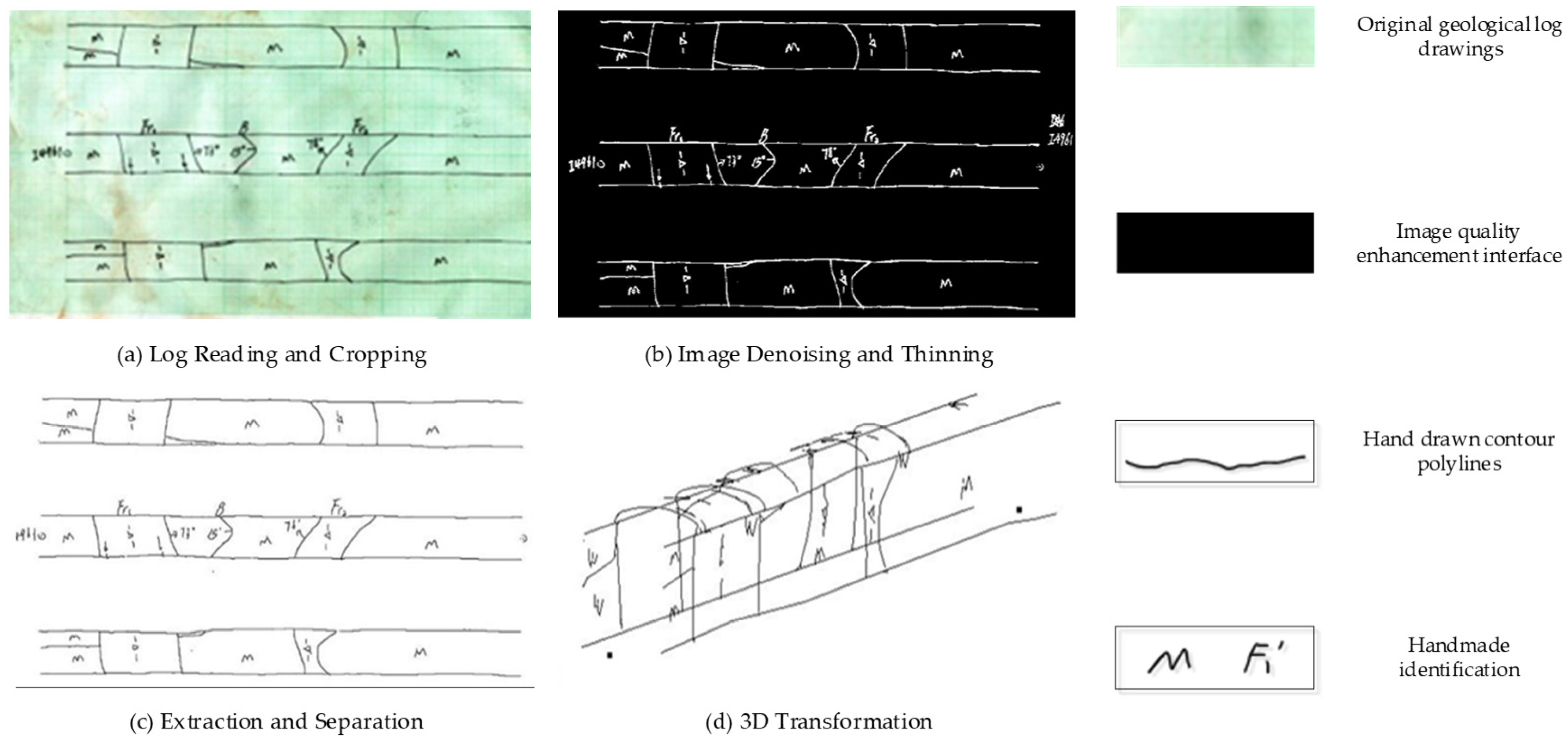
To obtain reliable vectorized polylines, we realized an image recognition-based vectorization method [33] for raw geological logging data. The method involves four main steps to convert scanned original geological logs into vectorized 3D geological boundaries for implicit modeling. The vectorization processes can be summarized as follows, as shown in Figure 2.

4.1. Scanning and Cropping

In the initial step, we should scan the target region from the original geological log drawings, followed by file compression. Since the raw logs contain non-graphical elements like text and labels, an interactive approach is used to manually crop the specific sections of the image that require vectorization, thus preparing the data for subsequent processing.

4.2. Image Denoising and Thinning

Based on the OpenCV tool, the cropped image undergoes quality enhancement through grayscale conversion, background blurring, and noise removal. The key denoising steps include bimodal threshold binarization after bilateral filtering, followed by single iterations of erosion and dilation. The cleaned image is then thinned to a single-pixel width skeleton using a combination of lookup table pre-processing and Rosenfeld post-processing to precisely represent the geological boundaries.

4.3. Extraction and Separation

Boundaries are extracted from the thinned image by tracing connected non-zero pixels, recording their coordinates, and resetting them to zero. The resulting complex lines are then simplified using the Douglas–Peucker algorithm [34] to reduce redundant points while preserving geometric shape, yielding key boundary points. Additionally, erroneously connected geological boundaries and tunnel roof lines are separated by breaking the line at inflection points, leveraging their characteristic large angle difference.

4.4. 3D Transformation

Leveraging the spatial relationships defined in the original log, along with actual engineering survey point coordinates, the vectorized 2D boundaries (including roof, floor, sidewalls, and geological features) are transformed into their true 3D positions through coordinate operations (translation, scaling, rotation) and projection, generating accurate 3D geological boundaries.

5. Cross-Contour Interpolation

The main difficulty of the orebody implicit modeling method based on contour polylines is to find a method that can automatically interpolate the normals of contour polylines according to the geometry shape characteristics of contour polylines. To estimate the normals of contour polylines dynamically, we consider transforming the problem of normal dynamic estimation of contour polylines into the problem of normal dynamic estimation of point clouds. However, compared with the traditional normal estimation problem of point clouds, the normal estimation problem of contour polylines needs to further consider the topological relationship of the contour polylines and the corresponding geometric continuity.

5.1. Normal Estimation

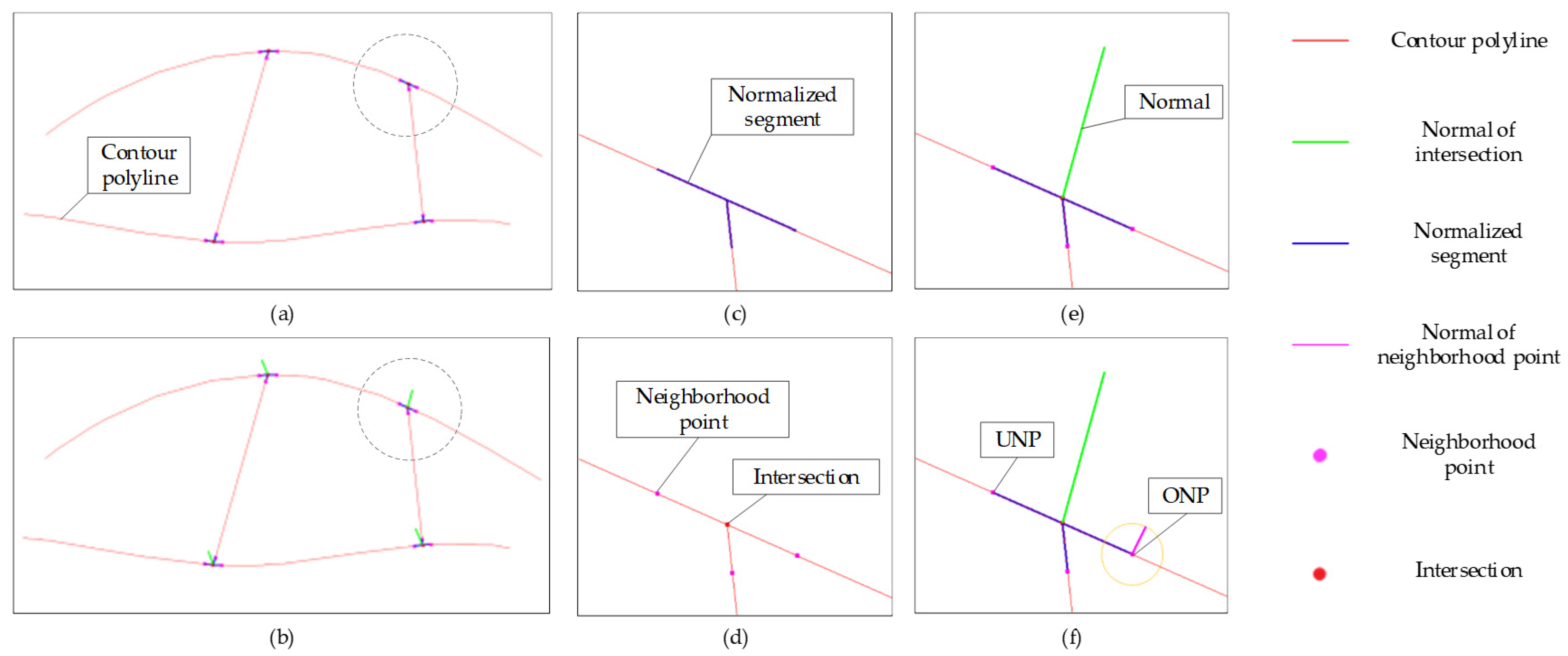
The step of normal estimation at intersection points estimates the normal of each segment using the improved principal component analysis (PCA) method according to the topology relationship of the intersecting polylines. Based on the idea of graph theory, a network graph $\mathit{G}(\mathit{V},\mathit{E})$ representing the topological adjacency relationship between polylines is constructed. The graph is defined by taking the intersection points of polylines as the nodes $\mathit{V}$ of the graph and taking the polylines as the edges $\mathit{E}$ of the graph, as shown in Figure 3.

Considering that some contour polylines have specified reliable normals, we present a dynamic normal estimation method to determine the normals of contour polylines using an improved PCA method. The basic idea of this method is to extract the neighborhood points normalized by the adjacent line segments at each intersection point to form the point cloud data, so as to transform the contour intersection normal dynamic estimation problem into the point cloud normal dynamic estimation problem. Different from the traditional point cloud estimation method, the point cloud normal dynamic estimation method can consider the influence of the prior oriented points on the normal estimation of the target intersection point.

It is worth noting that the extracted neighborhood points contain oriented and unoriented points. To clearly describe the process of dynamic normal estimation, we divide the neighborhood points of the target intersection point into unoriented neighborhood points (UNP) and oriented neighborhood points (ONP), as shown in Figure 3. Among them, the unoriented neighborhood points are composed of the points on the adjacent line segments without specified orientations at each intersection point, and the oriented neighborhood points are composed of points on the adjacent line segments with specified orientations at each intersection point. For a node (intersection point ${\mathit{x}}_0$) to be solved, suppose that there are $n$ unoriented neighborhood points ${\mathit{x}}_i(1\le i\le n)$ and $m$ oriented neighborhood points ${\mathit{x}}_j(1\le j\le m)$.

In the process of normalizing the weight of neighborhood points, the neighborhood point ${\mathit{x}}_i$ is determined by the following formula

$${\mathit{x}}_i={\mathit{x}}_0+{\mathit{l}}_i$$

(10)

where ${\mathit{l}}_i$ is the unitized line direction vector of the line segment adjacent to the corresponding intersection point.

In the case of normalizing the weight of the neighborhood points, the objective function formula of the improved PCA method can be defined as

$$\underset{‖\mathit{n}‖=1}{min}(\sum _{i=1}^n{(({{\mathit{x}}_i-{\mathit{x}}_0)}^T·\mathit{n})}^2+\sum _{j=1}^m{\left({\mathit{v}}_j·\mathit{n}\right)}^2)$$

(11)

where $\mathit{n}$ is the normal vector to be solved and ${\mathit{x}}_i=(x_i,y_i,z_i)$ are the unoriented neighborhood points at the corresponding intersection point. ${\mathit{v}}_j$ represents any one unitized vector orthogonal to the normal direction of the oriented neighborhood point ${\mathit{x}}_j$. ${\mathit{v}}_j$ satisfies

$$\left\{\begin{array}{c}{{\mathit{v}}_{\mathit{j}}·\mathit{n}}_j=0\\ ‖{\mathit{v}}_j‖=1 \end{array}\right., 1\le j\le m$$

(12)

Set

$${\mathit{y}}_i={\mathit{x}}_i-{\mathit{x}}_0$$

(13)

then

$$\underset{‖\mathit{n}‖=1}{min}(\sum _{i=1}^n{\mathit{n}}^T{\mathit{y}}_i{\mathit{y}}_i^T\mathit{n}+\sum _{j=1}^m{\mathit{n}}^T{\mathit{v}}_j{\mathit{v}}_j^T\mathit{n})=\underset{‖\mathit{n}‖=1}{min}({\mathit{n}}^T(\sum _{i=1}^n{{\mathit{y}}_i}^{\prime }{\mathit{y}}_i^{\prime T}+\sum _{j=1}^m{{\mathit{v}}_j}^{\prime }{\mathit{v}}_j^{\prime T})\mathit{n})$$

(14)

where ${{\mathit{y}}_i}^{\prime }={\lambda }_i{\mathit{y}}_i$, ${{\mathit{v}}_j}^{\prime }$ = ${{\lambda }_{j}d}_j{\mathit{v}}_j$.

$$\underset{‖\mathit{n}‖=1}{min}({\mathit{n}}^T(\sum _{i=1}^n{{\mathit{y}}_i}^{\prime }{\mathit{y}}_i^{\prime T}+\sum _{j=1}^m{{\mathit{v}}_j}^{\prime }{\mathit{v}}_j^{\prime T})\mathit{n})=\underset{‖\mathit{n}‖=1}{min}({\mathit{n}}^{\mathit{T}}\left(\mathit{Y}{\mathit{Y}}^{\mathit{T}}+\mathit{V}{\mathit{V}}^{\mathit{T}}\right)\mathit{n})$$

(15)

where $\mathit{Y}=[{{\mathit{y}}_1}^{\prime }{{\mathit{y}}_2}^{\prime }\dots {{\mathit{y}}_n}^{\prime }]$, $\mathit{V}=[{{\mathit{v}}_1}^{\prime }{{\mathit{v}}_2}^{\prime }\dots {{\mathit{v}}_n}^{\prime }]$.

Set

$$\mathit{C}=\mathit{Y}{\mathit{Y}}^T+\mathit{V}{\mathit{V}}^T$$

(16)

Then the final form of the objective function can be defined as

$$\begin{gathered} f\left(\mathit{n}\right)={\mathit{n}}^T\mathit{S}\mathit{n} \\ min\left(f\left(\mathit{n}\right)\right) \\ s.t.{\mathit{n}}^T\mathit{n}=1 \end{gathered}$$

(17)

Similar to the original PCA method, the normal vector at the intersection point can be estimated by solving the matrix $\mathit{S}$ using the eigenvalue decomposition method. And the normal vector $\mathit{n}$ to be solved corresponds to the smallest eigenvalue. After the normal vector of the intersection point is solved, the normal orientation of the line segment adjacent to the intersection can be calculated directly according to the projection relationship.

5.2. Normal Interpolation

The step of normal estimation for a single polyline interpolates the normals of the unoriented line segments according to the oriented line segments for each polyline using the linear interpolation method.

For a single polyline, there may be several line segments that have been assigned directions. To improve the accuracy of the normal estimation, the polylines with specified directions should be interpolated by the linear interpolation method before the normal estimation step at the intersection point. In this case, the polyline with the specified orientation will improve the normal estimation result of the adjacent polyline.

Set the tangent vector specified or estimated by the $u$-th segment of the polyline to ${\mathit{t}}_u$ and the tangent vector specified or estimated by the $v$-th segment to ${\mathit{t}}_v$. The formula of linear interpolation can be expressed as

$${\mathit{t}}_i=\left\{\begin{array}{c}{\mathit{t}}_u\times \left(1-{\displaystyle \frac{d_u}{d_u+d_v}}\right)+{\mathit{t}}_v\times {\displaystyle \frac{d_u}{d_u+d_v}}, {\mathit{t}}_u·{\mathit{t}}_v\ge 0\\ {\mathit{t}}_u\times \left(1-{\displaystyle \frac{d_u}{d_u+d_v}}\right)-{\mathit{t}}_v\times {\displaystyle \frac{d_u}{d_u+d_v}}, {\mathit{t}}_u·{\mathit{t}}_v<0\end{array}\right.$$

(18)

where ${\mathit{t}}_i$ and ${\mathit{l}}_i$ are the tangent vector and direction vector of the $i$-th segment to be interpolated of the polyline. $d_u$ is the distance from the $i$-th segment to the $u$-th segment, and $d_v$ is the distance from the $i$-th segment to the $v$-th segment.

The normal vector ${\mathit{n}}_i$ of the $i$-th segment to be interpolated can be expressed as

$${\mathit{n}}_i={\mathit{l}}_i\times {\mathit{t}}_i$$

(19)

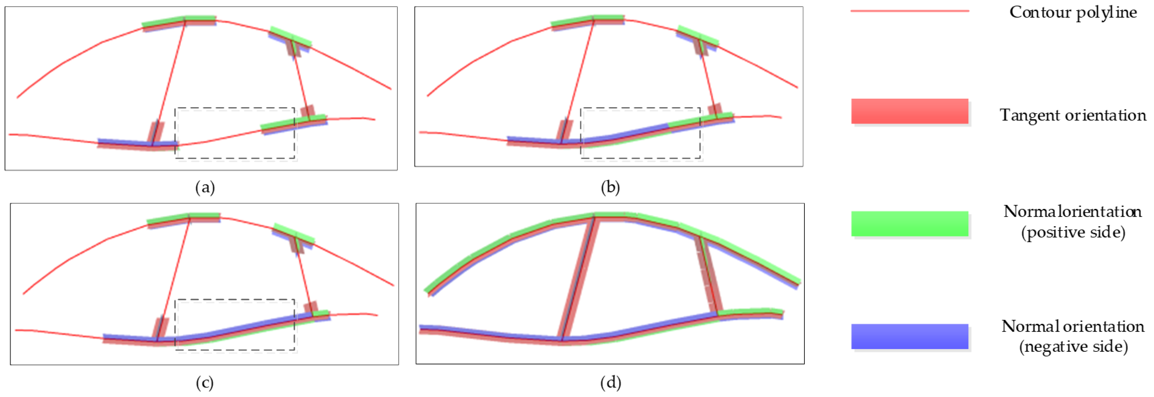
It is worth noting that the normal vector of the line segment calculated by the above method does not consider the positive or negative orientation of the normal, as shown in Figure 4. The step of normal reorientation of a single polyline ensures that the positive or negative normal orientation of each segment is consistent according to the shape trend between two adjacent segments of the polyline. Since the normal orientation of some segments already has a specified orientation, it is necessary to unify the normal orientation of orientation segment by segments.

Set the direction vectors and the estimated normal vectors of two adjacent segments of a polyline to ${\mathit{l}}_i$, ${\mathit{n}}_i$, ${\mathit{l}}_{i+1}$ and ${\mathit{n}}_{i+1}$. Generally, if ${\mathit{n}}_i$ is the reference normal vector (or manual specified normal vector), the reoriented normal ${\tilde{\mathit{n}}}_{i+1}$ should satisfy

$${\tilde{\mathit{n}}}_{i+1}=\left\{\begin{array}{c}{\mathit{n}}_{i+1}, {\mathit{t}}_i·{\mathit{t}}_{i+1}\ge 0 \\ {-\mathit{n}}_{i+1}, {\mathit{t}}_i·{\mathit{t}}_{i+1}<0\end{array}\right.$$

(20)

where

$$\left\{\begin{array}{c}{\mathit{t}}_i={\mathit{l}}_i\times {\mathit{n}}_i \\ {\mathit{t}}_{i+1}={\mathit{l}}_{i+1}\times {\mathit{n}}_i\end{array}\right.$$

(21)

It is worth noting that the normal reorientation process based on the above method is suitable for the condition that the vectors ${\mathit{l}}_i$, ${\mathit{n}}_i$, ${\mathit{l}}_{i+1}$ and ${\mathit{n}}_{i+1}$ are approximately coplanar. If the above vectors do not satisfy the approximate coplanar condition, we can convert the problem using the vector projection method. In special cases, when the process of normal reorientation is erroneous, it needs to rely on manual dynamic correction of the normal orientation.

5.3. Normal Reorientation

The step for reorienting normals for all polylines ensures that the normal direction of each polyline at the intersection is consistent according to the estimated normal at each intersection point. We reoriented the normals of the polylines by traversing the network graph by using the normal propagation algorithm.

To clearly describe the process of normal reorientation, we divided the polylines adjacent to the intersection point into unoriented adjacent polylines (UAP) and oriented adjacent polylines (OAP), as shown in Figure 5. Among them, the unoriented adjacent polyline represents a polyline without a specified normal direction that is adjacent to the intersection, and the oriented adjacent polyline represents a polyline with a specified normal direction that is adjacent to the intersection. The normal direction of an oriented adjacent polyline cannot be flipped.

Suppose that the solved normal vector at the intersection point ${\mathit{x}}_0$ is $\mathit{n}$ and the calculated normal vector of the $i$-th adjacent line segment is ${\mathit{N}}_i$; then, the reoriented normal vector ${\tilde{\mathit{N}}}_i$ of the $i$-th adjacent line segment should satisfy

$${\tilde{\mathit{N}}}_i=\left\{\begin{array}{c}{\mathit{N}}_i, \left(\mathit{n}·{\mathit{N}}_i\right)·\left(\mathit{n}·{\mathit{N}}_j\right)\ge 0\\ {-\mathit{N}}_i, \left(\mathit{n}·{\mathit{N}}_i\right)·\left(\mathit{n}·{\mathit{N}}_j\right)<0\end{array}\right.$$

(22)

where ${\mathit{N}}_j$ is the reference normal of a line segment adjacent to the intersection point.

When considering the existing direction of the polylines, the reference normal is determined based on the following criteria. If there are some oriented polylines that are adjacent to an intersection point, we will select the normal of any one oriented polyline as the reference normal; otherwise, we will select the normal of the polyline propagating to the current intersection point as the reference normal in the process of traversing.

There are two common traversing methods in the network graph as follows: the breadth-first search (BFS) and the depth-first search (DFS). After traversing, the propagation polylines and the intersection points form a spanning tree of the original network graph. The normal propagation process gradually corrects the normal orientations at each node according to the order in which the graph nodes of the spanning tree are traversed, as shown in Figure 6. In general, considering the propagation characteristics of the traversal process in the network graph, it is necessary to ensure that the graph nodes with high reliability are propagated first. It is useful to prevent the propagation of erroneous graph nodes from causing a large number of normal directions to be overturned.

Considering the existing orientation of the polylines, we utilized an improved BFS method to unify the normal orientation of all polylines. As this method optimizes the selection of the initial node of the original BFS method, it propagates the graph nodes and graph edges with higher reliability to reduce the erroneous propagation of normals. The specific steps of normal reorientation can be summarized as follows.

Step 1. A queue $\mathit{Q}$ in the searching process is constructed to store the graph nodes to be processed. The head and tail nodes corresponding to all polylines with specified orientation are added to the queue $\mathit{Q}$ as initial nodes.

Step 2. Take out the head element $V_i$ of the queue $\mathit{Q}$ in turn. Reorient the adjacent polylines at the node $V_i$ according to the solved normal vector at the corresponding intersection point.

Step 3. Mark the node $V_i$ and its adjacent polylines as processed to ensure that each polyline is reoriented only once.

Step 4. Obtain the other endpoints ${\mathit{V}}^{\prime }$ of the adjacent polylines of the node $V_i$. Sort the nodes ${\mathit{V}}^{\prime }$ according to the reliability of the estimation result.

Step 5. Traverse the nodes ${\mathit{V}}^{\prime }$. If $V_j^{\prime }\in {\mathit{V}}^{\prime }$ is not processed, add $V_j^{\prime }$ to the end of the queue $\mathit{Q}$.

Step 6. Take out the next head element of the queue $\mathit{Q}$. Return to Step 2 and repeat the searching process until all polylines are reoriented.

If the cross-contour normal dynamic estimation method is integrated into the 3D modeling software, some flexible interactive tools can be developed to update the normals of the contours dynamically. For geometrically complex polylines, it is useful to improve the accuracy of the normal estimation results. Taking the step of normal estimation for a single polyline as an example, interactive tools can be developed to adjust the normal orientation of a segment. In addition, for the step of reorienting normals for all polylines, interactive tools for freezing the estimated normals can be provided to ensure that the direction with reliable estimation results is not affected by subsequent update steps.

6. Experiments

6.1. Examples

To test the reliability of the orebody model dynamic updating method, we realized the proposed geological implicit modeling algorithm using the C++ programming language. We tested the dynamic normal estimation method on four groups of cross-contour polylines for orebody modeling, which were extracted from real-world geological logging data. To obtain the cross polylines efficiently, the datasets originated from scanned geological logs utilize the image recognition pipeline for vectorization.

To compare the original normal estimation method, we also demonstrated the interpolation result without specifying manual orientations. To obtain the modeling result, the implicit orebody modeling method [35], based on the radial basis functions interpolation method [16], was used to interpolate the oriented contour polylines, as shown in Figure 7, Figure 8, Figure 9, Figure 10 and Figure 11.

We have demonstrated the estimation result of our approach using the dynamic normal estimation method with and without manual orientations, as seen in Figure 7. There were several unexpected errors (which are marked by black lines) for the original normal estimation method without specifying manual orientations, as shown in Figure 7b. To avoid unexpected errors, we specified two oriented adjacent polylines, as seen in Figure 7c. Figure 7h shows that the errors are fixed by using the dynamic normal estimation method with manual orientations. The final modeling result was obtained by using the existing implicit modeling method, as shown in Figure 7i. The experimental results show that, for these cross-contour polylines with complex topological relationships, the results of estimating normals satisfy the expected effect by specifying the normals of some segments dynamically.

In addition, we compared the proposed method in this paper with the traditional explicit modeling method (Coons surface interpolation) on the same set of contour data. As demonstrated in Figure 8, as follows: (a) Explicit modeling requires section-by-section modeling of the contour data followed by manual stitching. This workflow is inefficient and induces discontinuities at the stitching boundaries, which manifest as step-like artifacts. (b) Our implicit method processes raw contours directly, constructing a unified continuous surface through the improved PCA method. It improves efficiency greatly while achieving a smooth, artifact-free surface. (c) The overlay comparison highlights that the explicit result (yellow mesh) exhibits stitching seams and geometric discontinuities, whereas our method (red surface) preserves the geological body’s continuous morphology.

More examples were tested to demonstrate the reliability of the dynamic normal estimation method for the cross-contour polylines, as shown in Figure 9, Figure 10 and Figure 11. Similarly, unconstrained estimation produces several obvious errors, including some flipped orientations. Based on our prior knowledge, we could fix the errors by specifying the normals of some segments dynamically. It is worth noting that some interactive tools can be developed to demonstrate the dynamic estimation effect and the dynamic modeling result.

6.2. Performance

The performance of the dynamic normal estimation method mainly depends on the number of intersection points and the number of contour polylines. We implemented the implicit orebody modeling algorithm based on the normal dynamic estimation of cross-contour polylines by using the C++ programming language. The algorithm was tested on a Windows 64-bit computer, which had a 3.70 GHz Intel (R) Core (TM) i7-8700U processor and 32 GB RAM.

Table 1. Experimental data statistics, including the intersection point number ($N_{pt}$), the polyline number ($N_{pl}$), the normal estimation time ($T_{ne}$), the number of segments assigned normals ($N_{se}$), the time of normal dynamic estimation ($T_{de}$), the total modeling time ($T_{to}$), and the Hausdorff distance (including $Min, Max, \mathrm{a}\mathrm{n}\mathrm{d} RMS$) between the models constructed by the method proposed in this paper and the standard PCA method.

Examples	${\mathit{N}}_{\mathit{p}\mathit{t}}$$/\mathit{n}$	${\mathit{N}}_{\mathit{p}\mathit{l}}$$/\mathit{n}$	${\mathit{N}}_{\mathit{s}\mathit{e}}$$/\mathit{n}$	Processing Time			Hausdorff Distance
				${\mathit{T}}_{\mathit{n}\mathit{e}}$$/\mathit{m}\mathit{s}$	${\mathit{T}}_{\mathit{d}\mathit{e}}$$/\mathit{m}\mathit{s}$	${\mathit{T}}_{\mathit{t}\mathit{o}}$$/\mathit{s}$	$\mathit{M}\mathit{i}\mathit{n}/\mathit{\%}$	$\mathit{M}\mathit{a}\mathit{x}/\mathit{\%}$	$\mathit{R}\mathit{M}\mathit{S}/\mathit{\%}$
Figure 7	39	63	2	1	1	4.18	0.00	0.59	0.06
Figure 9	76	123	2	1	1	1.95	0.00	4.86	0.74
Figure 10	38	65	4	1	1	6.50	0.00	2.77	0.33
Figure 11	40	66	3	1	1	2.48	0.00	3.63	0.28

reports the timings of the normal estimation algorithm and some of the corresponding parameters on the experiment examples.

The experimental results show that the proposed method can accurately estimate the normals of the overall cross-contour polylines according to the manually specified normals of some segments, and it can carry out implicit modeling based on the estimated normals. As the number of adjacent polylines of an intersection point is small, the orientations of the cross-contour polylines can be estimated efficiently. Moreover, compared with the original normal estimation method, there is no significant increase in the time of normal dynamic estimation ($T_{de}=T_{ne}$), and the total modeling time ($T_{to}$) is within 10 s. In addition, we also compared the model that was constructed by the method proposed in this paper with the model constructed using the standard PCA method and calculated the Hausdorff distance between them. The results are shown in Table 1.

While this method was developed and evaluated specifically for orebody modeling challenges, the core principles of contour-based surface reconstruction using normal estimation exhibit broader potential applicability. Notably, similar problems arise in medical imaging reconstruction from contour data, such as reconstructing 3D anatomical structures (e.g., organs, tumors, bones, etc.) from segmented contours in computed tomography (CT) or magnetic resonance imaging (MRI) slices. Beyond geology and medicine, contour interpolation problems with topological constraints are also found in computer-aided design (CAD) for automotive/aerospace parts, terrain modeling from bathymetric/isobathic lines, and paleontological reconstruction. Further research should explore the adaptability of our normal dynamic estimation and modeling framework. Domain-specific adaptation would, however, remain essential—medical contours demand extreme smoothness and anatomical fidelity, while orebody contours must adhere to structural geological controls.

7. Conclusions and Discussion

This study presents an innovative framework for dynamically updating 3D orebody models through the direct interpolation of geological logging data. By bridging critical gaps between geological interpretation and computational modeling, the method significantly advances the state-of-the-art in mineral resource estimation and mine planning workflows. As mining progresses toward autonomous operations, such dynamic geological modeling frameworks will form the essential digital substrate for adaptive mine planning and resource optimization.

The dynamic normal estimation algorithm for cross polylines using the improved PCA method enables robust implicit modeling while maintaining geological plausibility during incremental updates. The method can dynamically estimate the normals of contour polylines on the basis of manually specifying the normals of segments step by step, which can greatly improve the reliability of the results of the normal estimation. As the geometry position relationship between contours is integrated into interpolating normals, the original shape of the orebody can be recovered well in implicit modeling. The experimental results of several orebody modeling examples show that the method can be used to dynamically model the geological data set with a large number of complex contour polylines, which is useful for improving the automation of implicit orebody modeling and the reliability of implicit modeling results.

Based on the normal dynamic estimation of contour polylines, we can update the orebody dynamically using the implicit modeling method. However, this method still has some limitations that need to be further improved. Because the normal calculation at intersection points mainly depends on the point cloud normal estimation method based on PCA, the method is suitable for the surface modeling of smooth models. As the contour interpolation integrates the existing normals, the manually specified normals must be reliable enough to avoid affecting the accuracy of the normal estimation of the corresponding adjacent polylines. In the process of normal propagation, the propagation at a node with erroneous estimation results may lead to a large number of normal flipping errors. Therefore, it is necessary to study the method of automatically determining and modifying the nodes with erroneous normals to improve the accuracy of normal dynamic estimation and further improve the automation of implicit modeling.

In practical applications, we find that when the polylines are sparsely distributed or the shape of the orebody is significantly distorted or deformed, the standard estimation and reorientation of the polylines tend to lead to errors. This is an inevitable problem for interpolating sparse data. And the normal estimation method depends on the assumed condition that the geometry shapes of the contours satisfy the requirement of the local surface-fitting method. It is necessary to further optimize the normal direction estimation method for complex contour polylines in the future. Normal estimation results are more reliable where the contour polylines are dense and the gradient is gentle. On the contrary, there are great uncertainties in the normal estimation results in the positions where the contour polylines are sparse and the trend changes greatly. Core failures arise when data violate the PCA assumptions; however, interactive refinement ensures practical applicability. Our future work targets uncertainty-aware sampling to minimize manual inputs.