Article

Web System for Solving the Inverse Kinematics of 6DoF Robotic Arm Using Deep Learning Models: CNN and LSTM

by
Mayra A. Torres-Hernández
1,2,3,
Teodoro Ibarra-Pérez
1,
Eduardo García-Sánchez
2,
Héctor A. Guerrero-Osuna
2,
Luis O. Solís-Sánchez
2,* and
Ma. del Rosario Martínez-Blanco
2,3,*
1
Instituto Politécnico Nacional, Unidad Profesional Interdisciplinaria de Ingeniería Campus Zacatecas (UPIIZ), Zacatecas 98160, Mexico
2
Posgrado en Ingeniería y Tecnología Aplicada, Unidad Académica de Ingeniería Eléctrica, Universidad Autónoma de Zacatecas, Zacatecas 98000, Mexico
3
Laboratorio de Inteligencia Artificial Avanzada (LIAA), Universidad Autónoma de Zacatecas, Zacatecas 98000, Mexico
*
Authors to whom correspondence should be addressed.
Technologies 2025, 13(9), 405; https://doi.org/10.3390/technologies13090405
Submission received: 30 May 2025 / Revised: 21 August 2025 / Accepted: 1 September 2025 / Published: 5 September 2025
(This article belongs to the Special Issue AI Robotics Technologies and Their Applications)

Abstract

This work presents the development of a web system using deep learning (DL) neural networks to solve the inverse kinematics problem of the Quetzal robotic arm, designed for academic and research purposes. Two architectures, LSTM and CNN, were designed, trained, and evaluated using data generated through the Denavit–Hartenberg (D-H) model, considering the robot’s workspace. The evaluation employed the mean squared error (MSE) as the loss metric and mean absolute error (MAE) and accuracy as performance metrics. The CNN model, featuring four convolutional layers and an input of 4 timesteps, achieved the best overall performance (95.9% accuracy, MSE of 0.003, and MAE of 0.040), significantly outperforming the LSTM model in training time. A hybrid web application was implemented, allowing offline training and real-time online inference under one second via an interactive interface developed with Streamlit 1.16. The solution integrates tools such as TensorFlow™ 2.15, Python 3.10, and Anaconda Distribution 2023.03-1, ensuring portability to fog or cloud computing environments. The proposed system stands out for its fast response times (1 s), low computational cost, and high scalability to collaborative robotics environments. It is a viable alternative for applications in educational or research settings, particularly in projects focused on industrial automation.

1. Introduction

A robot is an intelligent machine that primarily performs monotonous or unsafe tasks for human intervention [1,2]. Today, robots are very popular in various applications, from manufacturing to medical surgery [3,4,5]. A robotic arm is a programmable mechanical arm that can execute the functions of a human arm. To achieve this task, its programming is increasingly required to stop being static. More flexible programming is needed to make decisions and even perform precise and automatic adjustments and calibration during its operation [6,7]. This, in the last decade, has significantly increased research on the design of robotic arms that have used artificial intelligence algorithms to solve kinematics [8,9,10,11]. Kinematics is one of the bases for solving the problem of robotic arm motion and is divided into two types: direct and inverse [12,13]. The inverse kinematics solution is one of the most critical problems in robotic control because this solution provides the angles of the joints of a robotic arm from the desired positions to the final executor [14,15]. However, inverse kinematics solutions have some disadvantages, such as the solutions may not exist or have multiple solutions and the calculation will be more complex when the number of joints of the robotic arm increases, counting nowadays with advances in the use of artificial intelligence (AI) algorithms that allow addressing this problem effectively [16,17]. Recently, there has been a growing interest in machine learning for solving inverse kinematics problems in robotic manipulation [18,19,20,21,22,23].
Deep learning (DL) is an advanced machine learning (ML) technique that enables hierarchical learning through multiple levels of representation in deep architectures. Deep neural networks (DNNs), inspired by the structure of the human brain, consist of interconnected elementary units called neurons, which collectively form networks capable of modelling highly nonlinear relationships [24]. These architectures have proven to be particularly effective in addressing complex regression and classification tasks, such as the inverse kinematics (IK) problem in robotic manipulators with multiple degrees of freedom (DoF) [25].
Integrating DNN models into IK resolution enables overcoming several limitations inherent to traditional analytical or numerical methods, including high computational cost, low robustness to structural variations in the robot, and poor scalability to more complex robotic systems [26,27]. However, for DL-based solutions to be effectively deployed in industrial automation contexts, it is essential to develop robust models and integrate technological platforms that facilitate their usage, monitoring, and continuous updating [28].
The motivation behind the development of this project is to provide a software tool that is highly suitable for controlled environments in academic laboratories and research centers with limited financial resources, where access to advanced technologies is required without incurring high infrastructure or licensing costs.
In this context, web-based systems have emerged as a strategic solution for the deployment of intelligent models, offering accessible, efficient, and scalable platforms for real-time interaction in academic, research, and industrial settings. These systems enable users to access advanced functionalities directly through web browsers, eliminating the need for locally installed specialized software and ensuring cross-platform compatibility. This approach is particularly advantageous for rapid deployment in scenarios aligned with Industry 4.0, where flexibility, interoperability, and responsiveness are essential. Furthermore, web architectures facilitate centralized maintenance, continuous model updates, and the use of interactive interfaces, enhancing user experience while minimizing the computational load on client devices.
The integration with Fog Computing (FC) and cloud computing (CC) infrastructures enables distributed processing capabilities and real-time data management, positioning this model as an ideal framework for the autonomous control of robotic arms
This work presents the development, training, and validation of two DL models based on Convolutional Neural Networks (CNNs) and Long Short-Term Memory (LSTM) architectures, aimed at solving the inverse kinematics problem of the Quetzal robotic arm, a six-degrees-of-freedom (6-DoF) manipulator designed for educational and research purposes. The training dataset was generated using the Denavit–Hartenberg (D-H) model, and regularization techniques were employed to mitigate overfitting and improve the generalization capabilities of the models. Validation was performed through cross-validation and statistical methods, using standard evaluation metrics such as Mean Squared Error (MSE), Mean Absolute Error (MAE), and accuracy.
The aim is to integrate the deep learning (DL) models into an interactive web application developed with Streamlit, enabling online inference from desired end-effector positions and returning the corresponding joint angles, which are compared against those generated using the Denavit–Hartenberg (D-H) model. The system was implemented in Python, utilizing specialized libraries such as TensorFlow™ and Keras for neural network modelling, while the Anaconda® environment facilitated the management of virtual environments and dependencies. This technological setup ensures the system’s portability to distributed computing environments, positioning the proposed solution as a precise, scalable, and viable alternative, from its current prototype stage for academic or research purposes to its potential deployment in real-world industrial automation scenarios.

2. Materials and Methods

The first challenge addressed in the development of this research was the appropriate selection of hardware and software resources, guided by criteria such as processing capacity, compatibility, connectivity, and low cost. This initial phase was essential to ensuring the project’s technical feasibility, which involved implementing deep learning models and their integration into a functional and efficient web interface.

2.1. Software

The system’s conceptualization began with creating a conceptual diagram to identify the main layers, their functional objectives, and the technological tools required for their development. In this layered architecture [29], the Presentation Layer (or frontend) is responsible for the user interface and interaction, enabling the dynamic visualization of model predictions and real-time user input. The Application Layer (business logic layer) manages the core functionality, including data processing and deep learning model inference. Finally, the Data Layer (or persistence layer) manages datasets using structured data representations derived from the Quetzal robotic arm and stored in CSV files.
Based on this analysis, a comparative evaluation of Python-based frameworks and tools was conducted, selecting those that provided a robust and specialized environment for data science, neural network modelling, and web deployment [30], as illustrated in Figure 1.
Figure 1 describes the implemented software tools. Python 3.10 was chosen as the core programming language due to its widespread adoption in data science and artificial intelligence projects, as well as its rich ecosystem of libraries for data processing, visualization, machine learning, and graphical interface development. Among the selected tools, the following stand out:
Anaconda® Distribution 2023.03-1 a Python distribution designed for data science and artificial intelligence application development. It was primarily used for virtual environment management through conda, ensuring dependency compatibility among key libraries.
Spyder 6: an integrated development environment (IDE) optimized for data science in Python. It served to program, debug, and execute the neural network training scripts. Its integration with libraries like TensorFlow™ 2.15, NumPy, and Pandas and real-time visualization capabilities enabled an efficient and well-organized workflow [31].
Streamlit 1.16: an open-source framework for rapid development of interactive web applications. Its seamless integration with Spyder scripts enabled the design of an intuitive graphical interface for end users, supporting real-time data loading, interactive visualization, and execution of neural network predictions through a web platform [32].
The combination of these tools enabled the establishment of a modular development architecture: Anaconda® for environment management, Spyder for model construction and training, and Streamlit for the web interface.
Additionally, specialized libraries such as TensorFlow™ and Scikit-learn were employed to implement, train, and validate deep learning models. Other libraries supported data manipulation, analysis, visualization, and export. Figure 2 summarizes the libraries used [33].
This modular approach ensures system scalability, maintainability, and efficient integration of AI functionalities into a web-based application.

2.2. Hardware

The hardware used for all stages of this project, including dataset generation, data preprocessing, deep learning model training, and web system development, was a workstation equipped with a 10th-generation Intel® Core™ i7 processor and 16 GB of RAM. The limitations of this hardware setup were carefully considered during each phase, guiding the design decisions and the implementation of strategies to ensure efficient execution within the available computational resources.
In the present research, the Quetzal robotic arm employs six-degrees-of-freedom (6 DoF) manipulators developed for academic and research purposes. This robot features a detailed CAD model, a documented control flow, and functional simulations previously designed and described in the thesis by Ibarra et al. [34]. That work focused on creating an open-source manipulator, fabricated using 3D printing, with assembly, instrumentation, and a comprehensive mathematical analysis of its kinematics.
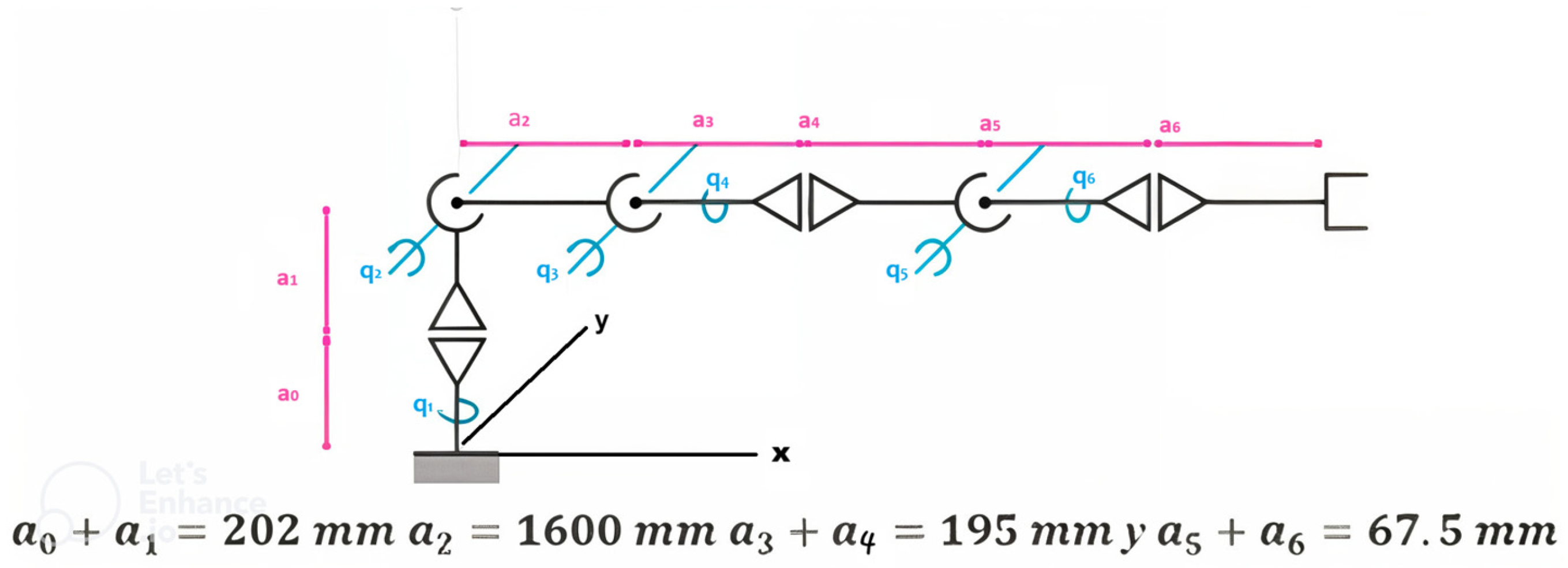
The Quetzal robotic arm presents a yaw-roll-roll-yaw-roll-yaw joint configuration, reaches a vertical height of 625 mm, and can handle payloads of up to 750 g. Its structure was designed in FreeCAD, using PLA for most structural components, while critical parts subjected to higher mechanical stress were printed in ABS, ensuring an optimal balance between lightness and mechanical strength. These features make Quetzal a flexible, low-cost, and lightweight manipulator, ideally suited for laboratory environments and for developing experiments related to automation, simulation, and the validation of robotic control algorithms. Figure 3 illustrates this process.
In that study, a finite dataset was generated by mapping the position and orientation coordinates of the end-effector to the corresponding joint values using the Denavit–Hartenberg (D-H) method, based on the geometric characteristics of the Quetzal arm, to obtain its workspace. Although the solution space is theoretically infinite, it was bounded by a spatial resolution of [ θ ] = ( θ 1 , θ 2 , θ 3 , θ 4 , 5 , θ 6 ) = 25 × 25 × 25 × 25 × 25 × 25, resulting in a total of 244,140,625 samples, achieving a balance between precision and computational feasibility, see Figure 4.
After the Quetzal robotic arm was 3D printed and physically assembled, the next stage involved simulating and validating its kinematics behaviour to ensure correct motion execution. For this purpose, a graphical representation of the manipulator was developed using the Robotics Toolbox for MATLAB®, see Figure 5.
This robotic platform optimized training datasets and tuned structural parameters in Backpropagation neural networks in previous studies. The optimal parameters selected include 100 neurons in the first hidden layer and 30 neurons in the second hidden layer, with a momentum value of 0.01 and a learning rate of 0.1. The training process was completed in 17.19 min using a dataset comprising 24,414 samples. The final results yielded an MSE of 0.06 and a data validation accuracy exceeding 89%, applying a robust design methodology inspired by Genichi Taguchi’s design philosophy to solve the inverse kinematics problem. A complete analysis of the data flow, training dataset generation, results, and simulations is published in the work of Ibarra et al. [35].
Instead, this study focuses on designing, training, and evaluating deep learning models applied to the exact inverse kinematics problem and their integration into a web-based system.

2.3. Methodology

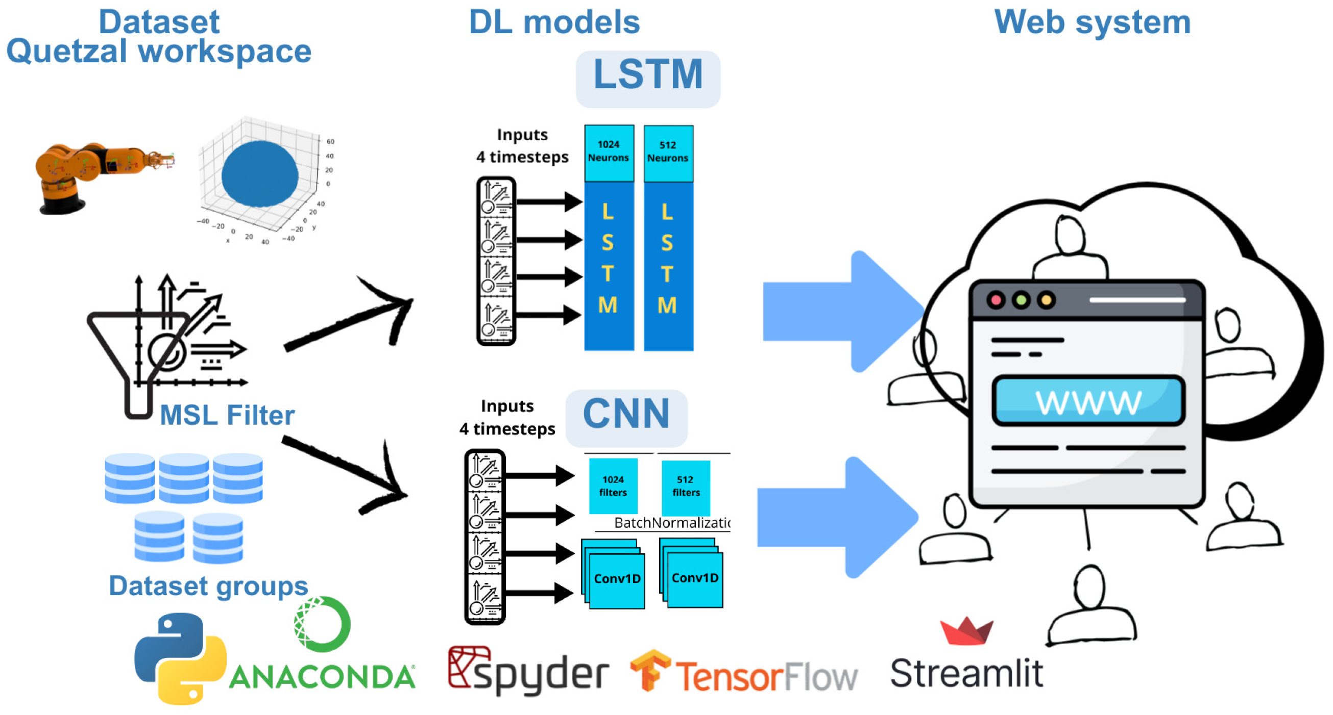
The methodology designed for developing the Web System, which integrates two deep learning models: CNN and LSTM, for solving the inverse kinematics problem and enables the comparison of their results with those obtained using the Denavit–Hartenberg (D-H) method, is presented in Figure 6.

2.3.1. Dataset Quetzal Workspace

All possible combinations of end-effector positions and orientations were obtained from the dataset of 244,140,625 inverse kinematics samples generated using the Denavit–Hartenberg (D-H) method. These samples were defined through the position vectors {px, py, pz} and orientation vector [n o a] = {nx, ny, nz, ox, oy, oz, ax, ay, az} which served as input variables for training the deep learning models. Each input was associated with its corresponding joint angles θ 1 , θ 2 , θ 3 , θ 4 , θ 5 , θ 6 . It was constrained based on the geometric characteristics of the robot, with the corresponding motion ranges defined as shown in Table 1.
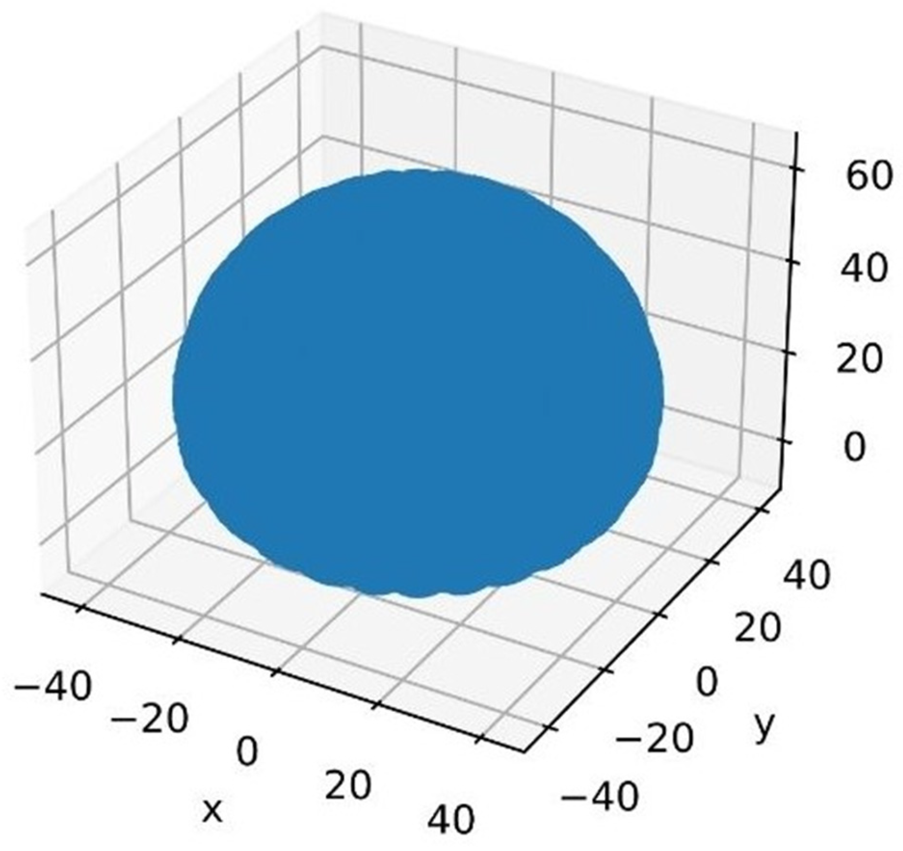
Figure 7 shows the graph of the position vector values, which forms a comprehensive and detailed knowledge base for inverse kinematics inference.
However, the data volume had to be reduced due to computational constraints and the need to ensure efficiency during the training phase. To achieve this, a linear systematic sampling (LSS) technique was applied, allowing for the extraction of representative subsets from the full dataset. This method preserved the diversity and coverage of the input space while minimizing the introduction of selection bias.
As a result, up to five data subsets were created, each containing 100,000 samples. These subsets were structured as sequential inputs (timesteps) and used to train the CNN and LSTM models, following the configurations specified in Table 2.
This timesteps based data organization enabled efficient training and facilitated the learning of relevant spatial and temporal patterns necessary for accurate joint angle inference.

2.3.2. Initial Model Design of CNN

Convolutional Neural Networks are a specialized architecture within the field of deep learning. They are primarily designed to process data structured in a grid-like topology, such as two-dimensional images or one-dimensional time series [36]. Their strength lies in their ability to automatically extract hierarchical representations and local features through trainable filters applied across convolutional layers [37].
While CNNs have been traditionally applied to image processing, they have also proven effective in analyzing temporal signals or multivariate sequential data through the use of 1D convolutions, making them well-suited for modelling spatial and temporal dependencies in tasks such as inverse kinematics resolution in robotics.
The initial development phase focused on evaluating baseline architectures composed of 3 to 6 one-dimensional convolutional layers (Conv1D), trained on a dataset of 100,000 samples with a single-timestep input structure. A comprehensive hyperparameter search was conducted, experimenting with activation functions such as ReLU, LeakyReLU, ELU, tanh, and SeLU; batch sizes of 32 and 64; and optimization algorithms including Adam and SGD. The training process aimed to minimize the loss (MSE) and enhance evaluation metrics such as MAE and prediction accuracy by increasing the number of training epochs and the architectural complexity through deeper layer stacking, as illustrated in Figure 8. Although early results demonstrated improved fitting to the training data, the models exhibited evident overfitting, particularly in performance degradation on validation data, underscoring the need for architectural adjustments and the incorporation of regularization strategies to enhance generalization.

2.3.3. Initial Model Design LSTM

Long Short-Term Memory (LSTM) networks are a specialized architecture within the field of deep learning, specifically designed to model sequential data and learn long-range dependencies over time. LSTMs incorporate memory cells and gating mechanisms (input, forget, and output gates) that enable them to retain or discard information selectively across time steps. This capability allows LSTMs to capture complex sequences’ short-term and long-term temporal dependencies.
LSTM networks have demonstrated strong performance in processing multivariate temporal data in control systems, signal interpretation, and robotics. Their capacity to model the dynamic behaviour of sequential inputs makes them well-suited for solving inverse kinematics problems, where capturing temporal coherence between positional and angular data is essential for accurate joint angle prediction in robotic manipulators.
In this model, baseline LSTM architectures consisting of one to three stacked LSTM layers were evaluated and trained on the same dataset of 100,000 samples using a single-timestep input configuration. Various hyperparameters were tested, including activation functions such as ReLU, LeakyReLU, and tanh; batch sizes of 32 and 64; and optimization algorithms such as Adam and SGD. The training process aimed to minimize the loss of MSE and improve evaluation metrics such as MAE and prediction accuracy by increasing the number of training epochs and the architectural complexity through LSTM layer stacking, as illustrated in Figure 9.
Although performance metrics showed progressive improvement on the training set, the model exhibited a clear tendency toward overfitting, as evidenced by performance degradation on the validation set. This behaviour mirrored that observed in the initial CNN model, as shown in Figure 10, highlighting the need for a refined design to achieve better generalization and more robust learning performance.

2.3.4. Overfitting Mitigation Techniques

Increasing the dataset using temporal sequences (Timesteps): using temporal sequences, or timesteps, in recurrent models such as LSTM and CNN, is an effective strategy to expand both the volume and quality of the training dataset. Segmenting the data into smaller overlapping sequences makes generating multiple training instances from a single dataset possible. This approach efficiently enlarges the training data in a compact form, enhancing the model’s ability to predict, detect anomalies, recognize patterns, and forecast trajectories [38,39,40]. As previously described in the data preparation section, training for the proposed CNN and LSTM models included datasets structured into sequences of 3, 4, and up to 5 timesteps, which were used as input to the model’s first layer.
The TimeDistributed layer: plays a key role in managing complex sequence-based problems in LSTM and CNN architectures, particularly when training on temporal data. Its use has significantly improved model accuracy in tasks focused on classification and prediction [41]. The TimeDistributed layer enables the application of the same operation, such as a Dense or Conv1D layer, independently to each timestep within a sequence, while preserving the temporal structure of the input [42,43].
In the models proposed in this study, the TimeDistributed layer was integrated immediately before the output layer. Such behaviour allowed a dense wrapper layer to be applied to each individual timestep of the input sequence, transforming its dimensionality and returning an output that maintains the same number of timesteps. Crucially, this transformation preserved the sequential integrity of the data while delivering a single unified data structure to be processed by the final output layer.
This design proved essential for leveraging the full capabilities of the CNN and LSTM models in solving a recurrent regression problem, where the goal is to produce exactly six continuous output values—the joint angles (θ1, θ2, θ3, θ4, θ5, θ6).
Figure 11 shows a sample code configuration of the TimeDistributed layer used in the implementation.
EarlyStopping: it involves halting the training process once the model’s performance on the validation set ceases to improve, typically indicated by an increase in validation loss or a stagnation in a monitored metric such as validation accuracy. This approach helps avoid excessive fitting to the training data, which can degrade the model’s generalization performance on unseen data [44], as illustrated in Figure 12.
Recent research has confirmed that EarlyStopping is particularly effective when training advanced architectures such as LSTM and CNN, especially under computational resources and training time constraints. It reduces the overall training duration and enhances model stability in response to variations in input data, enabling efficient training without compromising robustness [45].
In this study, the application of EarlyStopping significantly improved the performance of the proposed LSTM and CNN models. Interrupting the training process before overfitting occurred effectively reduced generalization error, thus achieving better performance with fewer computational resources. The EarlyStopping mechanism monitors a specific validation metric, loss_val, at the end of each epoch. Training is automatically terminated if no improvement is observed after a predefined number of consecutive epochs, specified by the patience parameter. Additionally, the parameter restore_best_weights=True, ensures that the model reverts to the weights that yielded the best performance during training, further enhancing generalization capabilities [46]. The corresponding EarlyStopping configuration code is shown in Figure 13.
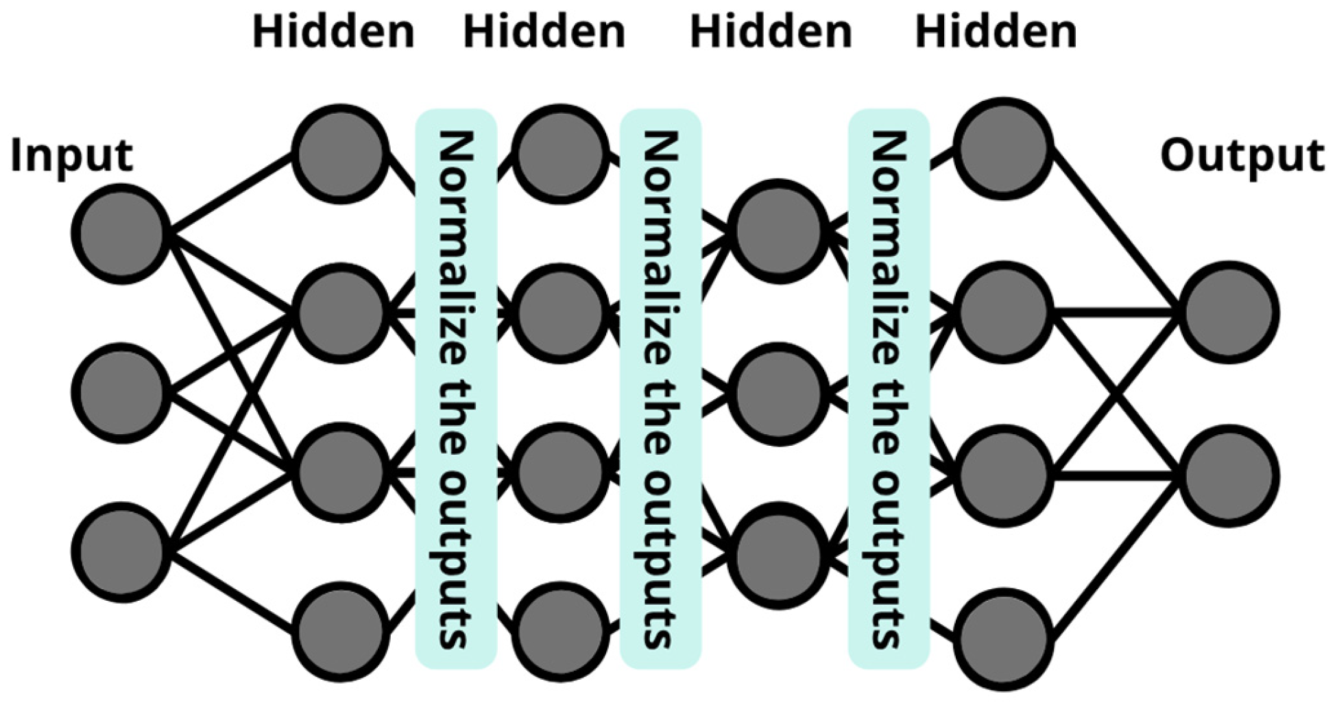
Batch Normalization (BN): This is a technique introduced by Ioffe and Szegedy in 2015 to enhance the speed, stability, and overall performance of training deep neural networks. Its primary goal is to mitigate the internal covariate shift, which refers to the changes in the distribution of layer activations as the network parameters are updated during training [47]. BN performs batch-wise normalization by applying a transformation that keeps the output mean close to 0 and the standard deviation close to 1. This normalization facilitates gradient propagation through the network, leading to faster convergence and more stable training dynamics [48], as illustrated in Figure 14.
In this project, BN is incorporated due to the highly variable nature of the input variables (e.g., angles and positions), which makes it challenging to detect consistent patterns. BN helps ensure that the input values of each mini-batch remain within a manageable statistical range (in terms of mean and variance) at each layer, ultimately contributing to improved accuracy and training stability in the proposed CNN and LSTM models.
Dropout: This is a regularization technique introduced by Srivastava et al. [49] to reduce overfitting in deep learning. It works by randomly deactivating a fraction of neurons in each layer during training. This random deactivation prevents neurons from becoming overly reliant on one another, thereby encouraging the learning of more robust and generalizable feature representations. During each training iteration, Dropout randomly selects a subset of neurons to be excluded from both the forward pass and Backpropagation. This stochastic behaviour forces the network to learn redundant representations of the input data, improving the model’s ability to generalize by reducing its dependency on specific patterns of neural activations, as illustrated in Figure 15.
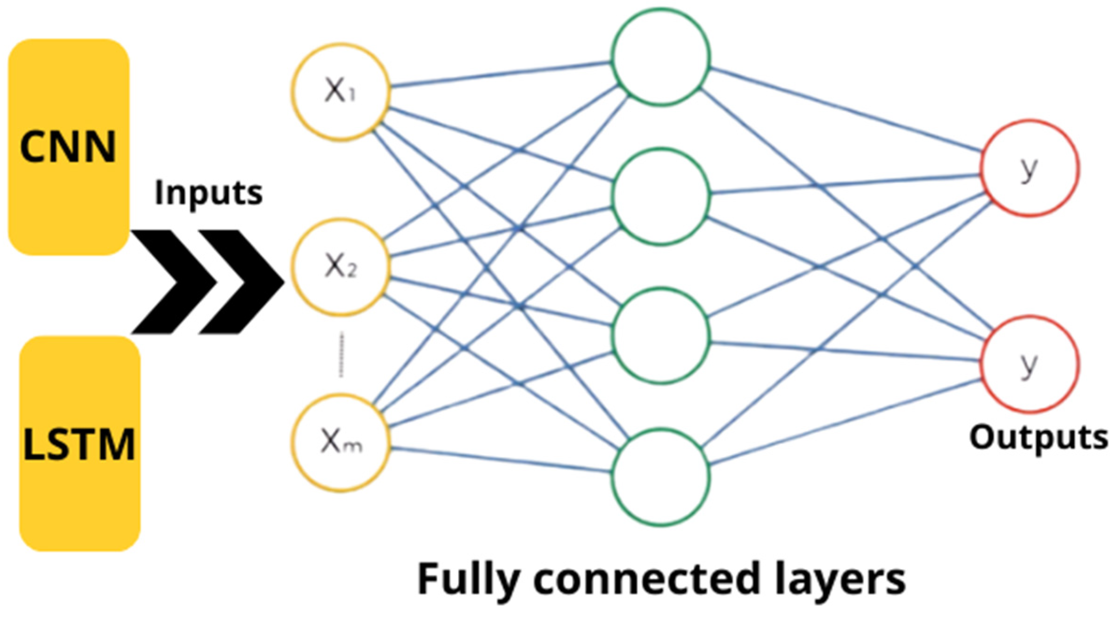
Fully connected (FC) layers: In these layers, each neuron is connected to every neuron in the previous and subsequent layers, forming a dense mesh of connections that allows for maximum information flow and modelling of complex, nonlinear relationships between inputs and outputs. Mathematically, a dense layer performs a linear transformation followed by a nonlinear activation function [50], as shown in Equation (1):
y = f(Wx + b),
where x is the input vector, W is the weight matrix, b is the bias vector, and f is the activation function (e.g., ReLU, sigmoid, tanh). This formulation enables the network to approximate highly nonlinear mappings, which is particularly valuable for robotics tasks like classification, regression, and inverse kinematics [51].
Fully connected layers are often used in the final stages of modern deep learning architectures to integrate features extracted by convolutional or recurrent layers, such as LSTM or CNN [52], as illustrated in Figure 16.

2.3.5. Final CNN Architecture

This final CNN model addresses a multivariable regression task by predicting continuous values corresponding to the six degrees of freedom of the Quetzal robotic arm. The architecture consists of multiple convolutional layers, normalization, regularization, and dense layers, designed to capture low- and high-level features from sequential multivariate data, as illustrated in Figure 17.
The structure and function of each component in the final CNN-based model are outlined below:
  • Input data: A sequence format of (4, 12) was selected, balancing model performance and training efficiency. Here, 4 represents the number of temporal steps, and 12 the number of features per timestep.
  • Convolutional layers (Conv1D): These layers scan through the temporal sequences using a kernel of size 3 to detect local patterns over time. The model includes four Conv1D layers with 1024, 512, 256, and 128 filters. The Swish activation function was applied in the first and third layers, and ReLU in the second and fourth, leveraging the complementary strengths of both activations.
  • Batch normalization: This was applied between each Conv1D layer to stabilize and accelerate training by normalizing the activations. This behaviour reduces issues related to input scale imbalances.
  • Dropout layers: this was used to prevent overfitting, with a rate of 0.1 between convolutional layers and 0.2 in the fully connected layers.
  • Fully connected layers: the model includes dense layers with 600, 400, and 200 neurons, each using the Swish activation function.
  • The model uses a loss function MSE, an Adam optimizer with a learning rate 0.001, and evaluation metrics MAE and accuracy to assess overall predictive performance.
  • Output layer: The model outputs six continuous values, representing the predicted joint angles (θ1, θ2, θ3, θ4, θ5, θ6) corresponding to the six degrees of freedom of the robotic arm.
Overall, this CNN architecture efficiently extracts both local and global features from multivariate sequential data through stacked convolutional layers with increasing filter complexity. The integration of normalization and regularization techniques ensures robust training and improved generalization.

2.3.6. Final LSMT Architecture

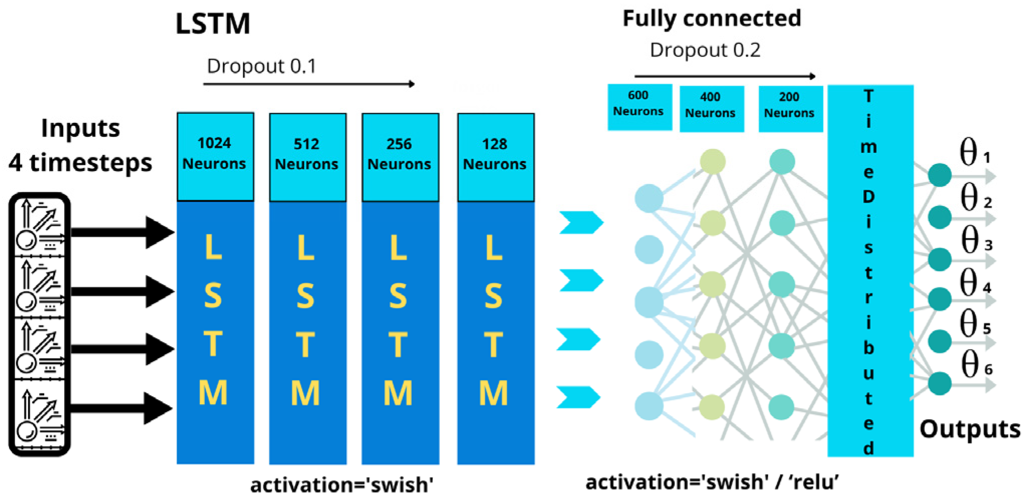
The final LSTM model developed in this study consists of stacked LSTM layers integrated with Dropout and dense layers. It is specifically designed to handle time-space prediction tasks with multivariate input-output relationships, as illustrated in Figure 18.
Each component of the architecture is detailed as follows:
  • Input data: a sequence shape of (4, 12) was selected to balance training efficiency and model performance, the same as the CNN model.
  • Stacked LSTM layers: four LSTM layers were used to allow the model to learn both short-term and long-term temporal dependencies. This deep, hierarchical structure enhances the network’s model of complex temporal patterns.
  • Fully connected layers: three dense layers with 600, 400, and 200 units were used, employing Swish activation in the first and third layers, and ReLU in the second.
  • Dropout layers: dropout rates of 0.1 were applied between LSTM layers and 0.2 between fully connected layers.
  • The time distributed layer, loss function, optimizer, evaluation metrics, and output layer are all the same as those in the CNN model.
The proposed CNN and LSTM architectures offer complementary advantages for solving the inverse kinematics regression problem. Both models effectively extract spatiotemporal features from the input data and demonstrate significant performance improvements by integrating overfitting mitigation techniques, such as batch normalization, dropout, and fully connected layers, as well as optimized hyperparameter configurations. These strategies collectively ensure robust performance and strong generalization capabilities across diverse input conditions.

2.3.7. Web System

A web system is a technological solution that enables user interaction with applications from any internet-connected device via a web browser. This implementation is particularly advantageous when deploying DL models, as it facilitates accessibility, remote data processing, and results visualization. Integrating LSTM and CNN models into a web platform leverages their capabilities to address problems such as the inverse kinematics of one or multiple Quetzal robotic arms, ensuring the tool is accessible to a wide range of users, as illustrated in Figure 19.
Furthermore, linking the system with emerging technologies such as the IoT, CC, and FC enhances its capacity for distributed processing, real-time data collection, and model availability in industrial environments. This technological architecture aligns with the principles of Industry 4.0.
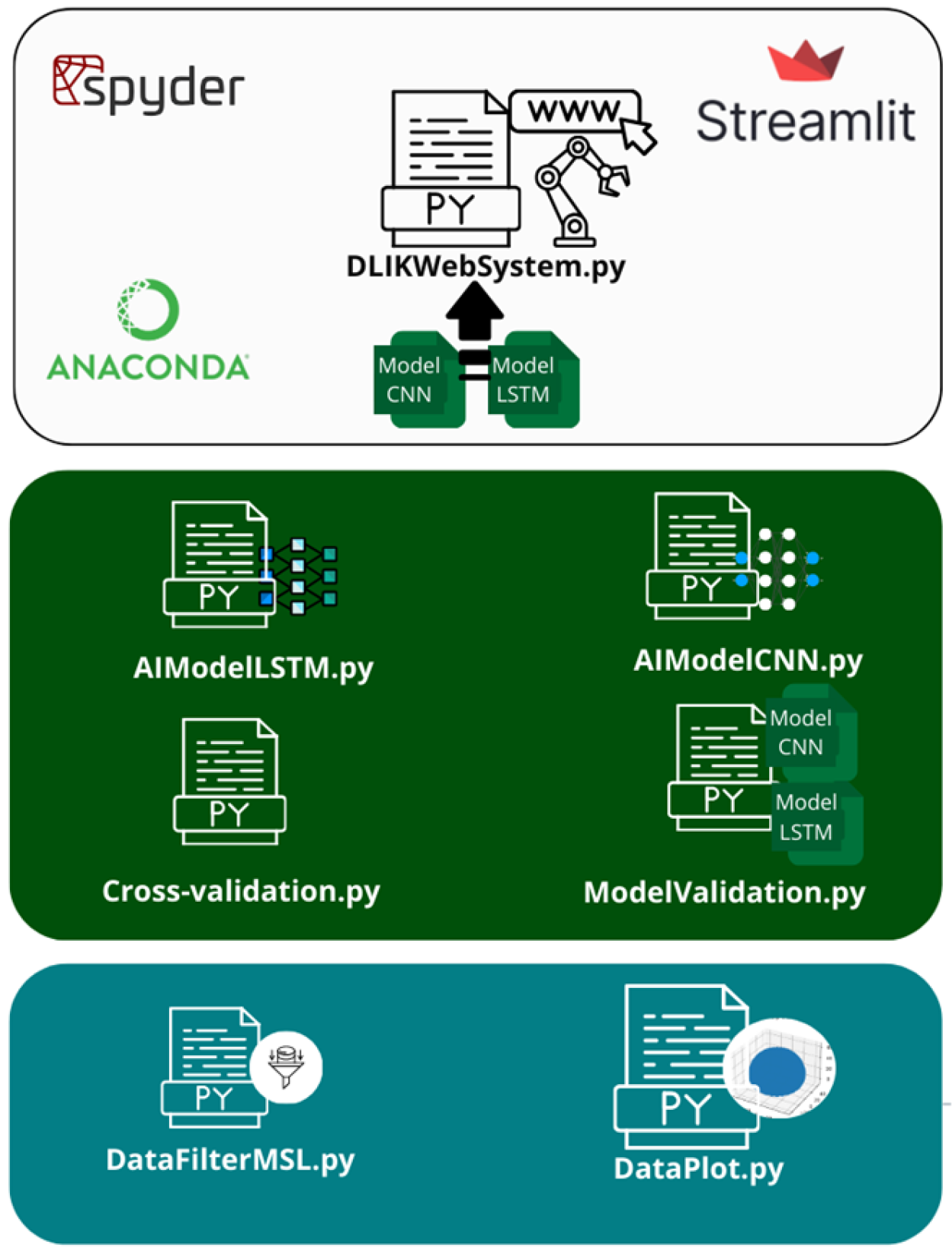
The web system was designed with a modular architecture to support scalability, maintainability, and component reuse. This modular structure is implemented through the functional division of the system into eight main Python scripts, as shown in Figure 20, enabling efficient integration of the DL models.
Python scripts enabled a modular and well-structured codebase, making the system easier to maintain and extend. Each script was designed to handle a specific task, facilitating debugging, updates, and adding new features without compromising system stability. The main functions of the scripts are:
  • DataFilterMSL.py: converts the Quetzal robot workspace from a .mat file to .csv, enabling easier data manipulation in Python. It applies a Systematic Linear Sampling (MSL) method to reduce dataset size while preserving spatial diversity, ensuring efficient DL model training.
  • DataPlot.py generates a 3D visualization of the filtered dataset using Matplotlib, allowing for spatial validation of the robot’s reachable workspace in X, Y, and Z space.
  • IAModelCNN.py & IAModelLSTM.py: Define the architecture, activation functions, input shapes, and training settings for the CNN and LSTM models. Once trained, the models are saved for real-time deployment in the web system to predict inverse kinematics.
  • CrossValidation.py: implements K-fold cross-validation to assess model robustness.
  • ModelValidation.py: evaluates model performance using MSE, MAE, R2, and Euclidean Distance by comparing predictions against a test set of 100,000 unseen samples, with ground truth generated via the Denavit–Hartenberg (D-H) method.
  • DLIKWebSistem.py: The main script that runs the web interface built with Streamlit.
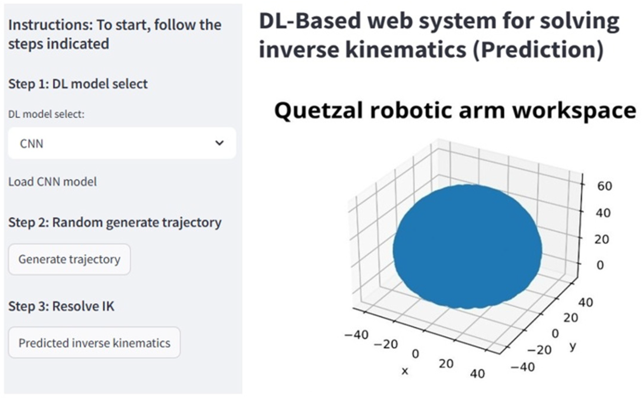
The developed web system provides an intuitive and accessible interface for interacting with the deep learning models used to solve the inverse kinematics of the Quetzal robotic arm. It features a sidebar that guides the user through three key steps: selecting the DL model (CNN or LSTM), inputting the target trajectory, and executing the inverse kinematics prediction. The system then displays evaluation metrics. This structure ensures usability for experts and non-specialized users, as illustrated in Figure 21.
This modularity supports agile and scalable development, particularly in complex environments such as artificial intelligence (AI) and robotics-based systems. Using the Anaconda® environment ensures efficient management of virtual environments and dependencies, enhancing compatibility and portability. Streamlit enables the rapid creation of interactive graphical interfaces, allowing for intuitive, low-cost web-based interaction with DL models.
These features make the system especially suitable for deployment in distributed environments like FC and CC, where real-time processing is needed despite limited resources. It also aligns with the requirements of Industry 4.0 cyber–physical architectures, which demand efficient integration of software, hardware, and intelligent networks for autonomous and highly responsive processes

3. Results

This section presents the results obtained from evaluating the performance of the DL models developed to solve the multivariable regression problem associated with the inverse kinematics of the Quetzal robotic arm. Key quantitative metrics are included, along with plots that illustrate the behaviour of both models during the training and testing phases. The analysis focuses on the best-performing models: the CNN and the LSTM network.
CNN model results: The initial CNN model was refined to improve generalization performance and mitigate overfitting observed during the first evaluation phase. The strategy focused on increasing the complexity of the input data by incorporating temporal sequences with three, four, and five timesteps. The network depth was expanded from three to four 1D convolutional layers (Conv1D), with filter sizes ranging from 32 to 1024. The layers employed ReLU, tanh, ELU, and swish activation functions.
Dropout layers were progressively added after each Conv1D layer to enhance regularization, with dropout rates decreasing from 0.5 to 0.1. All training experiments were conducted using the Adam optimizer with a learning rate of 0.001.
A key architectural component was the inclusion of fully connected layers, which integrate and consolidate features extracted by the convolutional blocks. These layers enable full connectivity between neurons in consecutive layers, allowing for nonlinear combinations of complex patterns, an essential capability for accurate inverse kinematics estimation. Between two and four dense layers were implemented with 32 to 1024 neurons, using ReLU, tanh, and swish activation functions.
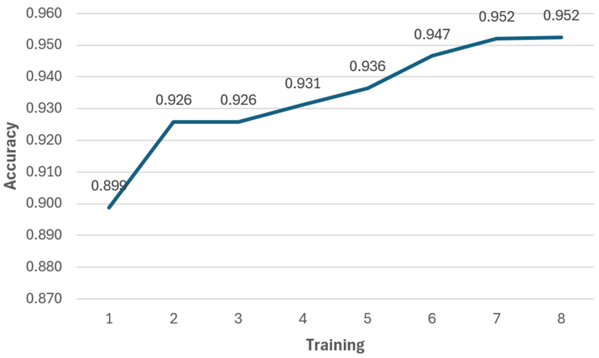
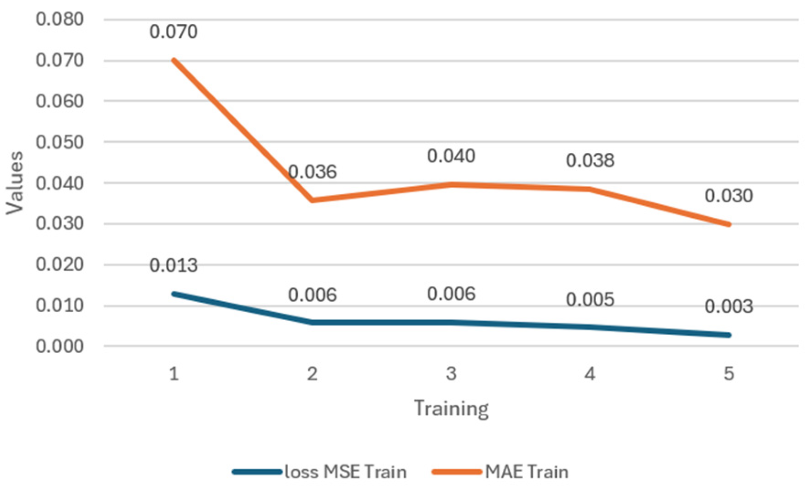
Furthermore, BatchNormalization layers were inserted after each Conv1D layer to stabilize activation and accelerate convergence during training. The hyperparameter configurations and training results for this model are summarized in Table 3, while performance trends are illustrated in Figure 22 and Figure 23.
The results demonstrate that the 4 timesteps CNN model exhibits superior generalization capability and lowers error margins in solving the inverse kinematics problem of the Quetzal robotic arm. These outcomes underscore the effectiveness of convolutional networks, especially when combined with overfitting mitigation techniques and well-structured architecture for regression tasks in robotic environments. In this context, the CNN model best suited for integration into the web system is the one represented in Figure 17 as it achieved an accuracy of 95.9%, an MSE of 0.003, and an MAE of 0.040, outperforming the 5 timesteps model’s 95.2% accuracy, 0.005 MSE, and 0.047 MAE. The hyperparameters used in both training configurations are detailed in Table 4.
The 4 timesteps model achieved a training time reduction of approximately 60.6% compared to the 5 timesteps model. Specifically, the 4 timesteps configuration required only 54 min to complete training, whereas the 5 timesteps model took 137 min under the same computational conditions. This significant improvement in training efficiency highlights the suitability of the 4 timesteps model for resource-constrained deployment scenarios.
LSTM model results: The temporal sequence length was also increased to 4 timesteps; this extension enabled the model to capture more complex and deeper temporal dependencies. A deeper architecture was designed, consisting of four LSTM layers with a decreasing number of units: 1024, 512, 256, and 128, respectively. Initially, the model’s performance was evaluated using the ReLU activation function, in combination with Dropout layers set at rates of 0.5, 0.2, and 0.3, aiming to mitigate the overfitting observed in previous configurations. However, integrating the swish activation function led to a significant improvement in performance metrics. This finding prompted further adjustments to the Dropout rates, reducing them to 0.2 and 0.1 to achieve a better balance between regularization and learning capacity.
An important finding was that including Batch Normalizationlayers between LSTM layers did not enhance training performance; instead, it adversely affected model convergence. This behaviour aligns with recent studies in the literature that highlight potential conflicts between batch normalization and the internal dynamics of LSTM cells, particularly when using smooth activation functions like swish. The refined configuration resulted in better model adaptation to the data characteristics. Table 5 presents some of the adjustments made to the model’s hyperparameter configuration, and their impact on performance is illustrated in Figure 24 and Figure 25.
When comparing the results obtained with 4 and 5 timesteps in the LSTM model, it becomes evident that the configuration using 4 timesteps delivered superior performance and greater training efficiency. This model achieved an accuracy of 96.2%, with an MSE of 0.002 and an MAE of 0.003, outperforming the 5 timesteps model, which reached an accuracy of 95.5%, an MSE of 0.006, and an MAE of 0.042. The detailed results are presented in Table 6.
Regarding training effort, the 4 timesteps model was trained for 134 epochs over 134.8 min, whereas the 5 timesteps model required 120 epochs but consumed significantly more time, 196.7 min. This represents a 31.5% reduction in training time when using 4 timesteps instead of 5. Despite requiring more epochs, the 4 timesteps model was notably more efficient, achieving better results with lower computational costs in less time.
Performance comparison of DL models: Both the LSTM and CNN-based architectures demonstrated high robustness in the developed models, each exhibiting distinct strengths. On the other hand, the LSTM model, while more time-consuming, leveraged its deep sequential architecture to capture complex temporal dependencies, achieving slightly better validation metrics accuracy 97%, MSE: 0.003, MAE: 0.030, than the CNN model accuracy 95%, MSE: 0.005, MAE: 0.047. Both models surpassed 94% accuracy on the test datasets, confirming their suitability for addressing the inverse kinematics problem of the Quetzal robotic arm in educational or research settings focused on industrial automation projects. These results are presented in Table 7.
The CNN model achieved high accuracy in significantly less time, requiring only 42 epochs and 54 min of training. This represents an 87.7% reduction in training time compared to the LSTM model, which required 439 min and 124 epochs. Such efficiency makes the CNN ideal for time or computational resource-constrained environments.
The final models were validated using rigorous k-fold cross-validation techniques, which allowed for a comprehensive assessment of their generalization capability across different data partitions. The results from the 5-fold cross-validation are presented in Table 8, and both the CNN and LSTM models demonstrated robust and consistent performance. Regarding MAE, the LSTM model showed a slightly lower value, 0.057, compared to the CNN, 0.067, suggesting a better average approximation of the expected outputs. However, the CNN outperformed the LSTM in MSE 0.0133 vs. 0.0144 for LSTM, and achieved a higher R2 0.996 vs. 0.991, indicating a greater proportion of variance explained by the model and a more accurate fit to the real data. Both models reached an average accuracy of 92%, reaffirming their overall effectiveness. Nevertheless, they differed in stability: CNN exhibited a lower standard deviation of 0.001 than the LSTM, 0.003, indicating more consistent behaviour across different validation folds. Overall, these results suggest that while the LSTM has a slight advantage in absolute error, the CNN stands out for its greater stability and explanatory power, which are key factors when considering implementation in robust prediction systems within real-world environments.
Additionally, quantitative validation tests were performed using metrics widely recognized in the scientific literature for evaluating deep learning models applied to regression tasks. Specifically, a combination of MSE, MAE, the R2, and Euclidean Distance (ED) was employed, and the thresholds and interpretations of performance metrics are presented in Table 9.
This set of metrics provides a holistic view of model performance, enabling standardized quantitative comparisons across different architectures and configurations. This evaluation strategy aligns with methodological frameworks described in works such as Goodfellow et al. [53], emphasizing the importance of rigorous and multifaceted model evaluation, particularly in scenarios requiring strong generalization to unseen data. Studies by Samarakoon et al. [54] and Halim et al. [55] further highlight the value of integrating statistical validations and quantifiable performance criteria to ensure model reliability in real-world applications.
To validate the generalization capability of the CNN and LSTM models, an independent dataset of 100,000 randomly selected samples, excluded from the training, testing, and validation sets, was generated. These samples represented target trajectories within the robotic arm’s workspace. The predictions of the CNN and LSTM models were applied to solve the inverse kinematics problem, and their predictions were assessed using the validation metrics detailed in Table 9. Results of the CNN model indicated that 96.76% of the predictions satisfied all established evaluation criteria. Subsequently, the same dataset was employed to evaluate the LSTM model’s performance, yielding 96.56% of predictions meeting the criteria. These outcomes demonstrate high accuracy and generalization for both CNN and LSTM models in addressing inverse kinematics within large-scale data contexts, as illustrated in Figure 26.
As the final stage of the validation process for the developed deep learning models, the 5-fold cross-validation and the quantitative validation using an external dataset of 100,000 samples confirmed the robustness and generalization capability of the CNN and LSTM architectures. The results demonstrated highly consistent and accurate performance across various scenarios. Specifically, the CNN architecture showed greater stability and computational efficiency, while the LSTM model exhibited slightly better performance in terms of absolute error. Both configurations surpassed the established validation thresholds, with over 96% compliance on unseen data, confirming their applicability in real-world contexts. Based on this comprehensive validation, the validated CNN and LSTM models were integrated into the developed web system; the implementation results are presented in the following section.
DL models significantly outperformed the results obtained with traditional neural networks, such as Backpropagation, in the initial research involving the Quetzal robotic arm. While the traditional approach employed a dataset of 24,414 samples, achieving an MSE of 0.06 and a prediction validation rate above 89% using Chi-square (χ2) statistical testing, the DL models were trained with a substantially larger dataset of 400,000 samples, which enabled a notable improvement in predictive performance. The DL models achieved an average MSE of 0.01, and following rigorous statistical validation, over 96% of the predictions met all the predefined evaluation criteria. These results demonstrate the superiority of DL architectures in solving the inverse kinematics problem of the Quetzal robotic arm, offering enhanced accuracy and generalization in complex operational scenarios.
Implementation of the web system: To interact with the deep learning models integrated into the web system, the user must follow three straightforward steps through the sidebar interface. First, the preferred model (CNN or LSTM) is selected according to the user’s requirements, as is illustrated in Figure 27.
Next, the final trajectory coordinates are entered into the designated input fields, as illustrated in Figure 28.
Alternatively, it can be generated by clicking the generated random trajectory button, as illustrated in Figure 29.
Suppose the user provides a trajectory point that falls outside the defined workspace limits of the robotic arm. In that case, the system will display an error message: “Limits of the robotic arm’s workspace reach: Limits x values: −40 to 40, Limits y values: −20 to 40, Limits z values: 0 to 60”. In such cases, the system will not proceed with the inverse kinematics calculation, ensuring that all operations remain within the robot’s feasible range of motion and preventing the generation of invalid or non-executable joint configurations, as illustrated in Figure 30.
Finally, the inverse kinematics prediction is executed, providing the resulting joint angles and the corresponding evaluation metrics. After clicking the “Predicted Inverse Kinematics” button, the system’s response has an average inference time of approximately 1 secondper sample for both models. Below is a complete execution example of the process using the CNN model, as illustrated in Figure 31.
Finally, Figure 32 illustrates a complete execution example of the process using the LSTM model.
The developed web system serves as a visual interface to close the results phase. It operates effectively as a predictive tool with an average response time of approximately 1 s per sample. This fast response capability represents a significant advantage for applications in industrial environments where near real-time interaction is required. The low latency in predicting and displaying joint angles allows for faster decision-making, improves the monitoring of robotic tasks, and enables the execution of robot movements almost in real time, eliminating the need for manual calculations or complex analytical solutions. Such capabilities provide substantial value in educational and research contexts focused on industrial automation.
On the other hand, while the LSTM model effectively captures sequential relationships, it shows slight variations in performance across different dataset partitions. This suggests that, for the specific problem of inverse kinematics in a 6-DoF robotic arm, the CNN architecture offers more predictable and reliable behaviour regarding generalization, sustained accuracy, and training efficiency.
The development of this web-based system offers significant advantages by integrating key capabilities such as multi-user operation, portability, and scalability—essential features for its adoption in academic and research environments aligned with Industry 4.0. These outcomes are the result of a strategic selection of specialized development tools: Python, for its versatility, simple syntax, and extensive ecosystem of libraries; Streamlit, which facilitates the creation of interactive web interfaces with rapid deployment and low hardware resource consumption; TensorFlow™, providing a robust and efficient environment for integrating deep learning models; and Anaconda, which optimizes the management of virtual environments and dependencies, simplifying system portability and maintenance.
The combination of these tools enabled the development of a web-based system capable of supporting simultaneous interaction from multiple users without performance degradation, making it particularly suitable for collaborative laboratories and academic or research settings. Additionally, the system demonstrates high portability, allowing rapid migration and deployment across different platforms or distributed infrastructures, such as Fog Computing or Computing environments, efficiently adapting to various operational conditions while minimizing deployment times.
Finally, its scalable architecture ensures progressive growth, allowing the integration of new models and functionalities without compromising the stability of the existing system. These features position the proposed solution as a flexible, robust, and sustainable platform, aligned with the automation and digitalization requirements of Industry 4.0, and well-suited for implementation in the scenarios addressed in this research. This positions the Quetzal arm as a valuable tool for education, research, and the prototyping of smart manufacturing processes, promoting the training of highly qualified human capital and supporting the transition to intelligent production systems.
An essential limitation of this project is that the experimental implementation of the web system directly on the Quetzal robotic arm has been designated as future work. Due to the limited availability of the hardware during this research phase, physical deployment and experimental tests on the real robotic system were impossible. As a result, the models could not be validated under real-world dynamic operating conditions, including aspects such as force control and real-time performance evaluation.
However, this project establishes a solid technological and methodological foundation, allowing future research stages to continue executing physical tests directly using the Quetzal robotic arm. Such an approach will evaluate system performance under real-life operating conditions and complete the validation cycle from simulation to practical implementation. The project also proposes integrating the system into an embedded circuit, allowing it to form part of a cyber–physical system, paving the way for research into collaborative robotics and advanced automation applications.

4. Discussion

The results of this research document the advantages of using DL models developed in Python to solve the inverse kinematics of a 6-DoF robotic arm in the context of Industry 4.0. Applying DL models such as CNN and LSTM proved an efficient, scalable, and viable alternative. They stand out for their generalization capacity and fast prediction performance compared to traditional methods like Denavit–Hartenberg (D-H), which require complex calculations.
The validity of the models was confirmed through 5-fold cross-validation and quantitative validation using statistical measures on a dataset of 100,000 simulated samples, achieving valid prediction rates above 96%. These results demonstrate their high performance and position them as suitable tools for academic and research environments in industrial automation.
In addition, a hybrid web application with local training and online prediction capabilities was developed, achieving inference times of one second. Using open-source tools (TensorFlow, Streamlit, Anaconda) enabled efficient integration and enhanced the system’s portability to fog or cloud computing environments.
Although physical testing with the Quetzal robotic arm was not possible, this phase is considered future work to validate the models under real conditions and move toward their integration into cyber–physical systems and IoT technologies within the Industry 4.0 ecosystem.

5. Conclusions

It was demonstrated that the developed solution constituted an accessible and efficient platform, capable of operating from a web server and being accessed from any device connected to the same network. These characteristics promote both interoperability and system accessibility. Furthermore, it was shown that DL-based models can overcome the limitations related to the amount of data typically required by traditional neural networks, such as the Multilayer Perceptron (MLP).
The CNN and LSTM architectures improved performance by applying overfitting prevention strategies, including regularization techniques and the appropriate selection of activation functions, ReLU and Swish. These strategies enhanced validation metrics such as MSE, MAE, and overall model accuracy.
A particularly notable outcome was the difference in training time: the CNN model required only 54 minutes, compared to the 439 minutes needed for training the LSTM model. This positions the CNN as the most efficient and suitable architecture for implementation in Industry 4.0 environments, where processing speed and rapid deployment are critical. This temporal efficiency is especially advantageous in scenarios requiring data retrieval and periodic retraining to continually improve model performance and adapt to new operational conditions. The generalization capability of the models was also validated through rigorous testing.
In addition to efficiently solving inverse kinematics, the developed system aligns with the core principles of Industry 4.0. The system was identified as having strong potential for evolution towards a cloud computing (CC) environment, enabling greater scalability, centralized maintenance, and continuous availability from any location. This technological architecture positions the system as an adaptable tool for cyber–physical and collaborative environments. The web system implemented in this research represents an initial approach to a cyber–physical system (CPS) focused on intelligent robotics.

Author Contributions

Conceptualization, M.A.T.-H. and M.d.R.M.-B.; Formal analysis, M.A.T.-H.; Investigation, M.A.T.-H., T.I.-P., L.O.S.-S. and M.d.R.M.-B.; Methodology, M.A.T.-H. and M.d.R.M.-B.; Project administration, L.O.S.-S. and M.d.R.M.-B.; Resources, M.A.T.-H., T.I.-P. and H.A.G.-O.; Software, M.A.T.-H., T.I.-P., L.O.S.-S. and M.d.R.M.-B.; Supervision, H.A.G.-O. and M.d.R.M.-B.; Validation, M.A.T.-H., T.I.-P., E.G.-S., L.O.S.-S. and M.d.R.M.-B.; Writing—original draft, M.A.T.-H. and E.G.-S.; Writing—review & editing, M.A.T.-H. and M.d.R.M.-B. All authors have read and agreed to the published version of the manuscript.

Funding

This work was supported by the Advanced Artificial Intelligence Laboratory and the Doctoral Program in Engineering and Applied Technology, with SNP recognition from CONAHCYT Mexico, National Polytechnic Institute, which supported this work under grant number CED/COTEBAL/38/2023.

Conflicts of Interest

The authors declare no conflicts of interest.

Abbreviations

DLDeep Learning
CNNConvolutional Neural Networks
LSTMLong Short-Term Memory
MSEMean Squared Error
MAEMean Absolute Error
FCFog Computing
CCCloud Computing
DoFDegrees of Freedom
LSSLinear Systematic Sampling
AIArtificial Intelligence

References

  1. Wang, Z.; Chen, D.; Xiao, P. Design of a Voice Control 6DoF Grasping Robotic arm Based on Ultrasonic Sensor, Computer Vision and Alexa Voice Assistance. In Proceedings of the 2019 10th International Conference on Information Technology in Medicine and Education (ITME), Qingdao, China, 23–25 August 2019; pp. 649–654. [Google Scholar] [CrossRef]
  2. Yasar, M.S.; Alemzadeh, H. Real-Time Context-Aware Detection of Unsafe Events in Robot-Assisted Surgery. In Proceedings of the 2020 50th Annual IEEE/IFIP International Conference on Dependable Systems and Networks (DSN), Valencia, Spain, 29 June–2 July 2020; pp. 385–397. [Google Scholar] [CrossRef]
  3. Velastegui, R.; Poler, R.; Díaz-Madroñero, M. Revolutionising industrial operations: The synergy of multiagent robotic systems and blockchain technology in operations planning and control. Expert Syst. Appl. 2025, 269, 126460. [Google Scholar] [CrossRef]
  4. Grischke, J.; Johannsmeier, L.; Eich, L.; Griga, L.; Haddadin, S. Dentronics: Towards robotics and artificial intelligence in dentistry. Dent. Mater. 2020, 36, 765–778. [Google Scholar] [CrossRef]
  5. Ashibani, Y.; Mahmoud, Q.H. Cyber physical systems security: Analysis, challenges and solutions. Comput. Secur. 2017, 68, 81–97. [Google Scholar] [CrossRef]
  6. Oyama, E.; Tachi, S. Inverse kinematics learning by modular architecture neural networks. In Proceedings of the IJCNN’99. International Joint Conference on Neural Networks. Proceedings (Cat. No.99CH36339), Washington, DC, USA, 10–16 July 1999; Volume 3, pp. 2065–2070. [Google Scholar] [CrossRef]
  7. Al-Hamadani, A.A.; Al-Faiz, M.Z. Design and Implementation of Inverse Kinematics Algorithm to Manipulate 5-DOF Humanoid Robotic Arm. In Proceedings of the 2021 International Conference on Innovation and Intelligence for Informatics, Computing, and Technologies (3ICT), Zallaq, Bahrain, 29–30 September 2021; IEEE: New York, NY, USA, 2021; pp. 693–697. [Google Scholar] [CrossRef]
  8. Alebooyeh, M.; Urbanic, R.J. Neural Network Model for Identifying Workspace, Forward and Inverse Kinematics of the 7-DOF YuMi 14000 ABB Collaborative Robot. IFAC Pap. 2019, 52, 176–181. [Google Scholar] [CrossRef]
  9. Chen, J.; Lau, H.Y.K. Learning the inverse kinematics of tendon-driven soft manipulators with K-nearest Neighbors Regression and Gaussian Mixture Regression. In Proceedings of the 2016 2nd International Conference on Control, Automation and Robotics (ICCAR), Hong Kong, 28–30 April 2016; pp. 103–107. [Google Scholar] [CrossRef]
  10. Karlik, B.; Aydin, S. An improved approach to the solution of inverse kinematics problems for robot manipulators. Eng. Appl. Artif. Intell. 2000, 13, 159–164. [Google Scholar] [CrossRef]
  11. Peng, Y.; Peng, Z.; Lan, T. Neural Network Based Inverse Kinematics Solution for 6-R Robot Implement Using R Package Neuralnet. In Proceedings of the 2021 5th International Conference on Robotics and Automation Sciences (ICRAS), Wuhan, China, 11–13 June 2021; IEEE: New York, NY, USA, 2021; pp. 65–69. [Google Scholar] [CrossRef]
  12. Karapetyan, V.A.; Miryanova, V.N. Solving the Inverse Kinematics Problem for a Seven-Link Robot-Manipulator by the Particle Swarm Optimization. In Proceedings of the 2023 International Russian Smart Industry Conference (SmartIndustryCon), Sochi, Russia, 27–30 March 2023; IEEE: New York, NY, USA, 2023; pp. 186–190. [Google Scholar] [CrossRef]
  13. Sharkawy, A.-N.; Khairullah, S.S. Forward and Inverse Kinematics Solution of A 3-DOF Articulated Robotic Manipulator Using Artificial Neural Network. Int. J. Robot. Control Syst. 2023, 3, 330–353. [Google Scholar] [CrossRef]
  14. Chen, H.; Chen, W.; Xie, T. Wavelet network solution for the inverse kinematics problem in robotic manipulator. J. Zhejiang Univ. Sci. A 2006, 7, 525–529. [Google Scholar] [CrossRef]
  15. Calzada-Garcia, A.; Victores, J.G.; Naranjo-Campos, F.J.; Balaguer, C. A Review on Inverse Kinematics, Control and Planning for Robotic Manipulators With and Without Obstacles via Deep Neural Networks. Algorithms 2025, 18, 23. [Google Scholar] [CrossRef]
  16. Cao, Y.; Wang, W.; Ma, L.; Wang, X. Inverse Kinematics Solution of Redundant Degree of Freedom Robot Based on Improved Quantum Particle Swarm Optimization. In Proceedings of the 2021 IEEE 7th International Conference on Control Science and Systems Engineering (ICCSSE), Qingdao, China, 30 July–1 August 2021; IEEE: New York, NY, USA, 2021; pp. 68–72. [Google Scholar] [CrossRef]
  17. Malik, A.; Lischuk, Y.; Henderson, T.; Prazenica, R. A Deep Reinforcement-Learning Approach for Inverse Kinematics Solution of a High Degree of Freedom Robotic Manipulator. Robotics 2022, 11, 44. [Google Scholar] [CrossRef]
  18. Aggogeri, F.; Pellegrini, N.; Taesi, C.; Tagliani, F.L. Inverse kinematic solver based on machine learning sequential procedure for robotic applications. J. Phys. Conf. Ser. 2022, 2234, 012007. [Google Scholar] [CrossRef]
  19. Calzada-Garcia, A.; Victores, J.G.; Naranjo-Campos, F.J.; Balaguer, C. Inverse Kinematics for Robotic Manipulators via Deep Neural Networks: Experiments and Results. Appl. Sci. 2025, 15, 7226. [Google Scholar] [CrossRef]
  20. Shakerimov, A.; Altymbek, M.; Koganezawa, K.; Yeshmukhametov, A. Machine learning-based inverse kinematics scalability for prismatic tensegrity structural manipulators. Robot. Auton. Syst. 2025, 193, 105102. [Google Scholar] [CrossRef]
  21. Joshi, R.C.; Rai, J.K.; Burget, R.; Dutta, M.K. Optimized inverse kinematics modeling and joint angle prediction for six-degree-of-freedom anthropomorphic robots with Explainable AI. ISA Trans. 2025, 157, 340–356. [Google Scholar] [CrossRef] [PubMed]
  22. Le, H.T.N.; Ngo, H.Q.T. Application of the vision-based deep learning technique for waste classification using the robotic manipulation system. Int. J. Cogn. Comput. Eng. 2025, 6, 391–400. [Google Scholar] [CrossRef]
  23. Phuc, T.D.; Son, B.C. Development of an autonomous chess robot system using computer vision and deep learning. Results Eng. 2025, 25, 104091. [Google Scholar] [CrossRef]
  24. Lab, E.A.I. Artificial Neural Networks vs Human Brain. Equinox AI Lab. Available online: https://equinoxailab.ai/neural-networks-vs-human-brain/ (accessed on 13 August 2025).
  25. Ogunmolu, O.; Gu, X.; Jiang, S.; Gans, N. Nonlinear Systems Identification Using Deep Dynamic Neural Networks. arXiv 2016, arXiv:1610.01439. [Google Scholar] [CrossRef]
  26. Johnson, C.C.; Quackenbush, T.; Sorensen, T.; Wingate, D.; Killpack, M.D. Using First Principles for Deep Learning and Model-Based Control of Soft Robots. Front. Robot. AI 2021, 8, 654398. [Google Scholar] [CrossRef]
  27. Omisore, O.M.; Han, S.; Ren, L.; Elazab, A.; Hui, L.; Abdelhamid, T.; Azeez, N.A.; Wang, L. Deeply-learnt damped least-squares (DL-DLS) method for inverse kinematics of snake-like robots. Neural Netw. 2018, 107, 34–47. [Google Scholar] [CrossRef]
  28. Heidari, A.; Navimipour, N.J.; Unal, M. Applications of ML/DL in the management of smart cities and societies based on new trends in information technologies: A systematic literature review. Sustain. Cities Soc. 2022, 85, 104089. [Google Scholar] [CrossRef]
  29. “Layered Architecture|AppMaster”. Available online: https://appmaster.io/glossary/layered-architecture (accessed on 12 August 2025).
  30. Lutz, M.; Python, L. Learning Python: Powerful Object-Oriented Programming, 5th ed.; O’Reilly Media, Inc.: Sebastopol, CA, USA, 2013. [Google Scholar]
  31. Anaconda; Inc. Learn More About Anaconda. Anaconda. Available online: https://www.anaconda.com/about-us (accessed on 31 March 2025).
  32. Streamlit; Inc. Streamlit • A Faster Way to Build and Share Data Apps. Available online: https://streamlit.io/ (accessed on 31 March 2025).
  33. Raschka, S.; Mirjalili, V. Python Machine Learning: Machine Learning and Deep Learning with Python, Scikit-Learn, and TensorFlow 2, 3rd ed.; Packt Publishing: Birmingham, UK, 2020. [Google Scholar]
  34. Ibarra-Pérez, T. Análisis, Diseño e Implementación de Tecnología Basada en Inteligencia Artificial para Resolver la Cinemática Inversa en un Manipulador Robótico de 6DoF. Ph.D. Thesis, Universidad Autónoma de Zacatecas, Zacatecas, Mexico, 2022. [Google Scholar]
  35. Ibarra-Pérez, T.; Ortiz-Rodríguez, J.M.; Olivera-Domingo, F.; Guerrero-Osuna, H.A.; Gamboa-Rosales, H.; del R, M. A Novel Inverse Kinematic Solution of a Six-DOF Robot Using Neural Networks Based on the Taguchi Optimization Technique. Appl. Sci. 2022, 12, 9512. [Google Scholar] [CrossRef]
  36. Avenash, R.; Viswanath, P. Semantic Segmentation of Satellite Images using a Modified CNN with Hard-Swish Activation Function. In Proceedings of the 14th International Joint Conference on Computer Vision, Imaging and Computer Graphics Theory and Applications, Prague, Czech Republic, 25–27 February 2019; SCITEPRESS-Science and Technology Publications: Setúbal, Portugal, 2019; pp. 413–420. [Google Scholar] [CrossRef]
  37. Sreekar, C.; Sindhu, V.S.; Bhuvaneshwaran, S.; Bose, S.R.; Kumar, V.S. Positioning the 5-DOF Robotic Arm using Single Stage Deep CNN Model. In Proceedings of the 2021 Seventh International Conference on Bio Signals, Images, and Instrumentation (ICBSII), Chennai, India, 25–27 March 2021; IEEE: New York, NY, USA, 2021; pp. 1–6. [Google Scholar] [CrossRef]
  38. Chandra, R.; Goyal, S.; Gupta, R. Evaluation of Deep Learning Models for Multi-Step Ahead Time Series Prediction. IEEE Access 2021, 9, 83105–83123. [Google Scholar] [CrossRef]
  39. Anggraeni, W.; Yuniarno, E.M.; Rachmadi, R.F.; Sumpeno, S.; Pujiadi, P.; Sugiyanto, S.; Santoso, J.; Purnomo, M.H. A hybrid EMD-GRNN-PSO in intermittent time-series data for dengue fever forecasting. Expert Syst. Appl. 2024, 237, 121438. [Google Scholar] [CrossRef]
  40. del Campo, F.A.; Neri, M.C.G.; Villegas, O.O.V.; Sánchez, V.G.C.; de J, H.; Jiménez, V.G. Auto-adaptive multilayer perceptron for univariate time series classification. Expert Syst. Appl. 2021, 181, 115147. [Google Scholar] [CrossRef]
  41. Montaha, S.; Azam, S.; Rafid, A.K.M.R.H.; Hasan, M.Z.; Karim, A.; Islam, A. TimeDistributed-CNN-LSTM: A Hybrid Approach Combining CNN and LSTM to Classify Brain Tumor on 3D MRI Scans Performing Ablation Study. IEEE Access 2022, 10, 60039–60059. [Google Scholar] [CrossRef]
  42. Zheng, Y. Hybrid Neural Network Models to Estimate Vital Signs from Facial Videos. BioMedInformatics 2025, 5, 6. [Google Scholar] [CrossRef]
  43. Karim, F.; Majumdar, S.; Darabi, H.; Harford, S. Multivariate LSTM-FCNs for time series classification. Neural Netw. 2019, 116, 237–245. [Google Scholar] [CrossRef]
  44. Prechelt, L. Early Stopping—But When? In Neural Networks: Tricks of the Trade; Springer: Berlin/Heidelberg, Germany, 1998; pp. 55–69. [Google Scholar] [CrossRef]
  45. Anam, M.K.; Defit, S.; Haviluddin, H.; Efrizoni, L.; Firdaus, M.B. Early Stopping on CNN-LSTM Development to Improve Classification Performance. J. Appl. Data Sci. 2024, 5, 312. [Google Scholar] [CrossRef]
  46. Chollet, F. Deep Learning with Python, Second Edition, 2nd ed.; Simon and Schuster: New York, NY, USA, 2021. [Google Scholar]
  47. Ioffe, S.; Szegedy, C. Batch Normalization: Accelerating Deep Network Training by Reducing Internal Covariate Shift. In Proceedings of the 32nd International Conference on Machine Learning, PMLR, Lille, France, 7–9 July 2015; pp. 448–456. Available online: https://proceedings.mlr.press/v37/ioffe15.html (accessed on 30 March 2025).
  48. Thakkar, V.; Tewary, S.; Chakraborty, C. Batch Normalization in Convolutional Neural Networks—A comparative study with CIFAR-10 data. In Proceedings of the 2018 Fifth International Conference on Emerging Applications of Information Technology (EAIT), Kolkata, India, 12–13 January 2018; pp. 1–5. [Google Scholar] [CrossRef]
  49. Srivastava, N.; Hinton, G.; Krizhevsky, A.; Sutskever, I.; Salakhutdinov, R. Dropout: A simple way to prevent neural networks from overfitting. J. Mach. Learn. Res. 2014, 15, 1929–1958. [Google Scholar]
  50. Xu, Q.; Zhang, M.; Gu, Z.; Pan, G. Overfitting remedy by sparsifying regularization on fully-connected layers of CNNs. Neurocomputing 2019, 328, 69–74. [Google Scholar] [CrossRef]
  51. Basha, S.H.S.; Dubey, S.R.; Pulabaigari, V.; Mukherjee, S. Impact of fully connected layers on performance of convolutional neural networks for image classification. Neurocomputing 2020, 378, 112–119. [Google Scholar] [CrossRef]
  52. Mohammed, E.U.R.; Soora, N.R.; Mohammed, S.W. A Comprehensive Literature Review on Convolutional Neural Networks. TechRxiv 2022, preprint. [Google Scholar] [CrossRef]
  53. Heaton, J. Ian Goodfellow, Yoshua Bengio, and Aaron Courville: Deep learning. Genet Program Evolvable Mach 2018, 19, 305–307. [Google Scholar] [CrossRef]
  54. Samarakoon, S.M.; Herath, H.M.; Yasakethu, S.L.; Fernando, D.; Madusanka, N.; Yi, M.; Lee, B.I. Long Short-Term Memory-Enabled Electromyography-Controlled Adaptive Wearable Robotic Exoskeleton for Upper Arm Rehabilitation. Biomimetics 2025, 10, 106. [Google Scholar] [CrossRef]
  55. Halim, M.Y.; Awad, M.I.; Maged, S.A. Hybrid Physics-Infused Deep Learning for Enhanced Real-Time Prediction of Human Upper Limb Movements in Collaborative Robotics. J. Intell. Robot. Syst. 2025, 111, 1–17. [Google Scholar] [CrossRef]
Figure 1. Layered model of the system.
Technologies 13 00405 g001
Figure 2. Python libraries.
Technologies 13 00405 g002
Figure 3. Quetzal robotic arm: (a) final assembly simulation in FreeCAD and (b) physically completed assembly.
Technologies 13 00405 g003
Figure 4. Graphical representation of the discrete joint angle configurations.
Technologies 13 00405 g004
Figure 5. Simulating and validating the Quetzal robotic arm: (a) modelled in FreeCADTM and (b) modelled in Robotics Toolbox for MATLAB®.
Technologies 13 00405 g005
Figure 6. Software development process and the technologies used.
Technologies 13 00405 g006
Figure 7. Dataset Quetzal workspace.
Technologies 13 00405 g007
Figure 8. Initial CNN base model.
Technologies 13 00405 g008
Figure 9. Initial LSTM base model.
Technologies 13 00405 g009
Figure 10. Tendency to overfitting models.
Technologies 13 00405 g010
Figure 11. Configuration of the TimeDistributed layer.
Technologies 13 00405 g011
Figure 12. EarlyStopping behaviour on training and validation errors.
Technologies 13 00405 g012
Figure 13. EarlyStopping configuration code.
Technologies 13 00405 g013
Figure 14. Workflow for applying Batch Normalization..
Technologies 13 00405 g014
Figure 15. Dropout behaviour.
Technologies 13 00405 g015
Figure 16. Workflow for applying fully connected layers.
Technologies 13 00405 g016
Figure 17. Final CNN model.
Technologies 13 00405 g017
Figure 18. Final LSTM model.
Technologies 13 00405 g018
Figure 19. Multi-user architecture of the web system.
Technologies 13 00405 g019
Figure 20. Set of scripts developed in Python.
Technologies 13 00405 g020
Figure 21. Main page of the web system.
Technologies 13 00405 g021
Figure 22. Result of the MSE and MAE metrics from training with 4 timesteps of the CNN.
Technologies 13 00405 g022
Figure 23. Result of accuracy from training with 4 timesteps of the CNN.
Technologies 13 00405 g023
Figure 24. Results of the MSE and MAE metrics from training with 4 time sequences of the LSTM network.
Technologies 13 00405 g024
Figure 25. Results of accuracy metrics from training with 4 timesteps sequences of the LSTM network.
Technologies 13 00405 g025
Figure 26. Threshold compliance summary.
Technologies 13 00405 g026
Figure 27. Steps for selection of models loaded in the system.
Technologies 13 00405 g027
Figure 28. Manually enter the position and orientation coordinates of the endpoint.
Technologies 13 00405 g028
Figure 29. Random generates the position and orientation coordinates of the endpoint.
Technologies 13 00405 g029
Figure 30. A trajectory point that falls outside the defined workspace limits of the robotic arm.
Technologies 13 00405 g030
Figure 31. Evaluation of the prediction with the CNN model vs. the traditional model (D-H).
Technologies 13 00405 g031
Figure 32. Evaluation of the prediction with the LSTM model vs. the traditional model (D-H).
Technologies 13 00405 g032
Table 1. Angular ranges in the joints of the Quetzal robotic arm.
(rad)θ1θ2θ3θ4 θ5 θ6
Minimum002π02π0
Maximum2πππ
2
2ππ
2
2π
Table 2. Generated data groups (timesteps) for training DL models.
# Timestep and % of Data from the Total SetTotal Data, Series Used, and Subsets Training—70%, Test 20%, and Validation 10%
1 Timestep
0.04%—100,000 Total
Technologies 13 00405 i001
100,000 total data distributed as follows:
70,000 training data
20,000 test data
10,000 validation data
3 Timesteps
0.12%—300,000 Total
Technologies 13 00405 i002
300,000 total data distributed in:
3 series of 100,000 with:
210,000 training data
60,000 test data
30,000 validation data
4 Timesteps
0.16%—400,000 Total
Technologies 13 00405 i003
400,000 total data distributed in:
4 series of 100,000 with:
280,000 training data
80,000 test data
40,000 validation data
5 Timesteps
0.20%—500,000 Total
Technologies 13 00405 i004
500,000 total
5 series of 100,000 with:
350,000 training data
100,000 test data
50,000 validation data
Table 3. The hyperparameter configurations.
#TrainDropoutConv1D Layers
and Filter
Activation
Functions
Fully Connected
Layers
10.3128-256-512-1024relu128–64
20.3-0.21000-800-400-600relu/swish600-400-200
30.5-0.3-0.21024-512-256-128swish600-400-200
40.5-0.3-0.2128-256-512-1024swish128-256
50.3-0.2128-256-512-1024relu128-256
60.3-0.21024-512-256-128relu/swish600-400-200
70.21024-512-256-128relu/swish600-400-200
80.11024-512-256-128relu/swish600-400-200
Table 4. Comparison of training results with the final CNN model’s 4 and 5 timestep sequences.
TimestepsEpochsTime (min)Loss MSEMAEAccuracy
442540.0030.04095.9%
5751370.0050.04795.2%
Table 5. Training with 4 timesteps for the LSTM model hyperparameter configuration.
# TrainingDropoutBatch_SizeActivation
Functions
LSTM Layers
No. Neurons
Fully Connected
No. Neurons
10.3-0.232relu128-256-51264-28
20.5-0.364swish1024-512-256256-512
30.3-0.264relu1024-512-256256-512
40.5-0.364swish1024-512-256200-400-600
50.1-0.264swish/relu1024-512-256600-400-200
Table 6. Comparison of training results with 4 and 5 timesteps of the final LSTM model.
TimestepsEpochsTime (min)Loss MSEMAEAccuracy
4134134.80.0020.00396.2%
5120196.70.0060.04295.5%
Table 7. Results of performance comparison of DL models.
DL
Model
EpochsTime
(min)
Accuracy
Train
Loss MSE
Train
MAE
Train
Accuracy
Test
Loss MSE
Test
MAE
Test
LSTM12443997%0.0030.0300.960.0080.035
CNN425495%0.0050.0470.940.0110.048
Table 8. Results from 5-fold cross-validation.
DL
Model
Average
MSE
Average
MAE
Average
R2
Average
Accuracy
Standard
Deviation
LSTM0.0140.0570.99692%0.003
CNN0.0130.0680.99192%0.001
Table 9. Thresholds and interpretations of performance metrics for quantitative validation.
Minimum Expected
Value of the Metrics
Indicates That
MSE < 0.03The prediction errors are small and consistent.
MAE ≤ 0.05 The average magnitude of the prediction errors is low, suggesting high accuracy.
R2 ≥ 0.9 The result explains a high proportion of the variance in the target data, reflecting strong predictive capability.
DE ≤ 0.5The predicted values are very close to the actual values in the multidimensional output space, ensuring high spatial precision.
Disclaimer/Publisher’s Note: The statements, opinions and data contained in all publications are solely those of the individual author(s) and contributor(s) and not of MDPI and/or the editor(s). MDPI and/or the editor(s) disclaim responsibility for any injury to people or property resulting from any ideas, methods, instructions or products referred to in the content.