Interplay of Connectivity and Unwanted Physical Interactions Within the Architecture of the D-Wave 2000Q Chimera Processor

Abstract

We consider dynamics relevant to annealing in qubit networks modelled on the architecture of the D-Wave 2000Q quantum processor (known as the Chimera topology). Our results report on the effects of the qubits’ connectivity and variable coupling strengths (based on physical interactions) on the dynamics of network. The networks we examine are up to 32 qubits in size and include coupling lengths varying by almost an order of magnitude. We show that while information transfer within the network can be strongly affected by the different interactions, the system maintains similar clusters of qubits with comparable fidelities even in the presence of some of the physical interactions. This suggests an intrinsic robustness of the Chimera topology to these perturbations, even if it includes such a variety of coupling lengths. Moreover, a similar clustering geometry was observed for other qubit properties in previous analysis of actual data from D-Wave 2000Q. This comparable behaviour suggests that the real quantum annealing chip is subject to little or no unwanted effects due to interactions that scale with the coupling lengths. This could be due to absence of the most damaging type of physical interactions and/or to D-Wave calibration methods tuning the control lines such that the couplings perform as if there is no effect due to their physical length. Our results are also relevant to the use of chaining for the creation of logical qubits. They show that even with very strong interactions between the chain, significant unwanted perturbations may occur due to the inhomogeneous fidelities of the overall dynamics and inhomogeneous dynamics should be expected for any given algorithm.

1. Introduction

Quantum computing is in its infancy and, as such, there is rapid development in a range of areas, with recent claims and predictions of quantum advantage and quantum supremacy [1,2,3]. One of the main stumbling blocks preventing vast scaling up of quantum computers are the errors in the devices that prevent them from executing circuits as programmed. These errors have a variety of causes, including manufacturing inconsistencies, poor isolation from the environment, and unwanted interactions between proximate qubits [4]. Some of these properties may be consistent across the system, but others vary between the individual qubits causing significant heterogeneity within the device [5]. It is challenging to attribute any effects seen in the execution of quantum computation to a particular source of error and therefore correct at the source. Simulations of devices with fabrication imperfections, for example, may help in this respect.

To correct or compensate for these problems, a number of error correction algorithms have been developed. These typically use a large number of duplicate qubits to preserve information through the circuit [6]. Although the error correction codes have been shown to be effective, the requirement of large numbers of extra qubits prevent them being applied on the limited size hardware options that are currently available.

The other approach to overcoming the systematic errors in quantum devices is to measure the errors and use these values to regularly re-calibrate the control signals that operate the device [7]. This works effectively, but is dependent on how often the calibration is performed and how far the qubits’ performance drifts between calibrations. For example, IBM quantum processors are calibrated both daily (calibration time of 30–90 min) and hourly (calibration time of 2–3 min) to ensure the most consistent performance for users [8].

In order to manage the heterogeneity in the system, it is necessary to characterise the qubits in as much depth as possible and to determine how robust each qubit might be to different types of error. If this information is known, it is likely that it will be possible to program the quantum device in such a way that the most robust qubits perform the most error-inducing steps. These are typically multi-qubit gates being run in parallel on nearby groups of qubits due to compounding errors in the individual qubits and the higher potential of crosstalk [9]. Furthermore, qubits may be robust only to errors of certain origin and their use in the circuit could be engineered to avoid the vulnerabilities in individual qubits and to exploit the heterogeneity in the system rather than to simply overcome it.

In a previous study, the authors identified spatial correlations in the properties of qubits in a D-Wave 2000Q quantum annealing chip [10]. This paper investigated the hypothesis that the physical layout of the chip is likely to affect the behaviour of the qubit network in unprogrammed ways. To investigate this, we wrote a simulation of the natural time evolution dynamics of a network of eight spins upon the insertion of a single excitation. The aim of the simulator was to consider how the physical layout of the qubits (and the potential interactions between them) affect the propagation of the excitation through the network. That research showed that the connectivity of a network can induce somewhat counter-intuitive and complex behaviour in the network. Given these results, we went on to hypothesise that this was at least partly due to the somewhat cyclical nature of the network and the lack of directionality in the couplings, leading to different possible paths (and related quantum interference) for the excitation to travel between any two qubits. Additionally, if the couplings have strengths that depend on their physical lengths, the dynamics become even more convoluted.

The work described here extends the findings detailed above. We use the same spin network simulator to compare the effects of different physical interactions generating qubit–qubit coupling: in addition to dipole–dipole interaction, we consider Coulomb coupling and an exponential interaction decay (in the linear regime). We also expand the analysis to 32 qubits in the D-Wave 2000Q (Chimera) topology. We compare results with a 32-qubit hypothetical bespoke architecture with a different connectivity profile to understand how the complex connectivity in the full quantum annealing chip could give rise to unprogrammed effects, as seen in a number of cases [11,12,13].

The structure of the paper is as follows. Section 2 summarises the theory of quantum annealing and the architecture of the D-Wave 2000Q quantum annealing chips. Section 3 sets out the methodology behind the simulator code and the calculation of the network time evolution. Section 4 and Section 5 use this simulator to further consider how the physical realisation of the qubit couplings might affect the dynamics of a D-Wave 2000Q quantum annealing device. This is acieved first by emulating the effects of using different qubit–qubit interactions to generate the strength of the networks’ couplings and then by considering networks of different sizes. Section 6 considers a bespoke network that has different connectivity to the D-Wave 2000Q chip considered previously. We use this to show how the connectivity in the network plays a key role in the behaviour of the qubits.

2. Theory

2.1. Quantum Annealing

Quantum annealing is a type of non-universal quantum computation used to solve optimisation and sampling problems using a partially connected network of qubits. Optimisation and sampling problems covers a range of real-world applications including travelling salesperson, image feature extraction, and solving Boolean multivariate equations [14,15,16]. For solving optimisation problems, the cost function and constraints first need to be transformed into an Ising Hamiltonian, representing the solution space as an energy landscape where the ground state is the optimal solution of the problem [17]. The qubit network begins in a general superposition state and is slowly transformed into the Ising Hamiltonian according to the equation

$$H={\displaystyle \frac{A\left(s\right)}{2}}{H}_A+{\displaystyle \frac{B\left(s\right)}{2}}{H}_B$$

(1)

with

$$H_A=\sum _i{\widehat{\sigma }}_i^x$$

(2)

and

$$H_B=\sum _i{h}_i{\widehat{\sigma }}_i^z+\sum _{i>j}{J}_{ij}{\widehat{\sigma }}_i^z{\widehat{\sigma }}_j^z$$

(3)

where s is normalised time ($s=t/t_f$, $0\le s\le 1$), and $t_f$ is the total annealing time. ${\widehat{\sigma }}_i^x$ and ${\widehat{\sigma }}_i^z$ are the X and Z Pauli matrices, respectively, acting on qubit i, and $h_i$ and $J_{ij}$ encode the problem as qubit biases and coupling weights, respectively. In practice, the $h_i$ and $J_{ij}$ are limited by the physical hardware graph (qubit–qubit connectivity; not all $J_{ij}$ are realisable directly) of the annealing device and the precision and accuracy of the circuitry controlling the qubits on the chip. For more details, see the review by Rajak et al. (2023) [18].

The Hamiltonian $H_A$ (Equation (2)) underpins the general superposition state (where all candidate solutions have equal probability), while $H_B$ (Equation (3)) is the Ising Hamiltonian that represents the problem to be optimised. At $t=0$, $s=0$, the system is initialised with $A\gg B$, so the first term in Equation (1) represents the system at the beginning of the annealing cycle. At the end of the annealing cycle, at $t=t_f$, $s=1$, the system has $B\gg A$, so it is represented by the problem Hamiltonian. If the intial state is the ground state of $H_A$ and the annealing cycle (decreasing A and increasing B) happens sufficiently slowly, the final state of the system is the ground state of the problem Hamiltonian $H_B$; the qubits can be read out to obtain the optimal solution [19].

The above description represents an ideal device, where the qubits form a closed system and the Hamiltonian in Equation (1) entirely describes the system and its dynamics. In reality, it is not feasible to completely isolate a quantum device from its environment and to completely control the interactions between the qubits. Therefore, there are a number of other terms in the actual enacted Hamiltonian, which represent interactions and energies that are not part of the programmed interactions but which can affect the system and may prevent it from reaching the ground state of the desired problem Hamiltonian. This study investigates the effects of some of these possible interactions that are not typically considered in quantum annealing but have the potential to change the dynamics of the system.

2.2. D-Wave Chimera Architecture

The largest commercial provider of quantum annealing devices is D-Wave, which produces several models with different numbers of qubits and different levels of connectivity [20]. The particular device whose architecture is emulated here is the 2000-Q system, which has 2048 qubits laid out in the ‘Chimera’ architecture. This architecture has unit cells of 8 qubits; each qubit is connected to 4 others within its unit cell and 2 qubits in neighbouring unit cells. Figure 1 shows a $2\times 2$ grid of unit cells. A full D-Wave 2000Q chip has a $16\times 16$ grid. The physical qubits are not circular as in the figure, but are elongated ovals, with qubits 0–3 in each unit cell horizontally oriented and 4–7 vertically oriented. So each qubit is connected to all of the oppositely oriented qubits within its unit cell and with two similarly oriented qubit from each neighbouring unit cell. Figure 1 only shows each qubit having one connection from a neighbouring unit cell but it is trivial to see how this pattern is extended to the full 16 × 16 grid. These connections between the qubits dictate which $J_{ij}$ terms in the annealing Hamiltonian (Equation (3)) can be non-zero.

Where the problem to be solved requires couplings that are not natively present in the architecture, a technique known as chaining can be employed to emulate the missing connections. Chaining involves coupling neighbouring physical qubits with very strong $J_{ij}$ values such that they behave as one logical qubit, and the connections of all the chained qubits can be used as if they were one qubit [22,23,24].

As noted above, in practice, qubits are not perfect and can be subject to errors, either from non-perfect manufacturing or from unwanted interactions with other qubits or the environment [25]. When the logical qubit needs to be measured, all the qubits in the chain are measured and a majority vote is taken. Determining the fidelity of a chain is challenging as using a majority vote can absorb some error within the chain, but there are also more qubits and couplers through which errors can be induced and transferred. There are no simple metrics published in the literature to assess the behaviour of a chain beyond looking at its behaviour as part of an algorithm as opposed to its physical behaviour [26,27]. Knowing more about the physical behaviour of individual qubits and couplings will enable more effective chaining of qubits through the chip. This is our motivation for studying the dynamics of a single excitation in the system here.

3. Methodology

Quantum annealing usually starts from the ground state of the Hamiltonian $H_A$ (Equation (2)), which is typically not an eigenstate of the problem Hamiltonian $H_B$ (Equation (3)). $H_B$ induces dynamics in the system, and in particular non-conservation of the original number of excitations (here, excitation refers to the single qubit eigenstate of ${\sigma }_x$ corresponding to a qubit in the state $|1\rangle$ of the standard basis) and their hopping between different qubits, as dictated by the hopping parameters $J_{ij}$. In this study, we focus on the dynamical aspect of this process, rather than the overall annealing process. Also, we ignore the bias term, so $h_i=0$, $\forall i$.

We investigate how the difference in physical location of the network of qubits (and hence their distances apart) and different physical kinds of coupling affect the dynamics. We use a bespoke simulator which takes as inputs a network or nodes, edges, and node positions, and an interaction type that defines how the hopping parameters $J_{ij}$ are related to the lengths of the edges to define a matrix version of the Hamiltonian

$$H_{xy}=\sum _{i>j}{J}_{ij}({\widehat{\sigma }}_i^x{\widehat{\sigma }}_i^x+{\widehat{\sigma }}_j^y{\widehat{\sigma }}_j^y).$$

(4)

This Hamiltonian induces excitations hopping between qubits with the same hopping parameter strength $J_{ij}$ of $H_B$. It also preserves the number of excitations in the network, allowing for simulation of larger clusters of qubits.

Imperfections and unwanted perturbations to the values of the $J_{ij}$ affect the dynamics in the networks used in quantum annealing. To understand this, we consider how the hopping parameters could be affected by physical interactions between qubits. The interaction types considered are constant coupling, Coulomb coupling, dipole-dipole coupling, and  exponential decay, with the mathematical forms given, respectively, by

$$J_{ij}=J_0$$

(5)

$$J_{ij}=J_0{\displaystyle \frac{r_{min}}{r_{ij}}}$$

(6)

$$J_{ij}=J_0{\left({\displaystyle \frac{r_{min}}{r_{ij}}}\right)}^3$$

(7)

$$J_{ij}=J_{0}exp(-k(r_{ij}-r_{min}))$$

(8)

where $r_{min}$ is the length of the shortest coupling in the network and $r_{ij}$ is the length of the coupling between nodes i and j. Hence $r_{min}\le r_{ij}$.

The constant k in Equation (8) is chosen to be $k=0.001$, which provides a rate of decay in the linear regime, giving a coupling strength dependency between the constant and Coulomb cases. This formulation is preferable to using an explicit linear relationship, removing the risk of negative coupling strengths with large $r_{ij}$ values. From now on, this type of coupling is referred to as ‘linear’.

The constant coupling (Equation (5)) acts as a control scenario. In all cases, the edge lengths are normalised such that the shortest link in the network has a coupling strength of $J_0$. Hence, all the $J_{ij}$ values are between 0 and 1, a range that could be handled in the D-Wave quantum annealing chip. In our simulations, we set $J_0=1$.

The process of generating the Hamiltonian is shown in the flowchart in Figure 2, and the equivalent pseudocode is in Algorithm 1. This calculates the $J_{ij}$ values for Equation (4) and returns the Hamiltonian as an $N\times N$ matrix (single-excitation subspace), where the diagonal terms represent the on-site energies (here set to 0) and the other terms are the coupling strengths $J_{ij}$. These are non-zero where there is an edge connecting qubits i and j, with a value that is dependent of the interaction type and coupling length. This Hamiltonian is the basis for the simulations presented here.

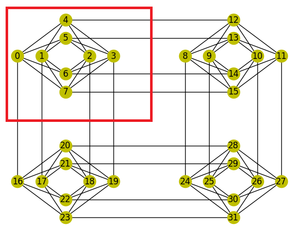
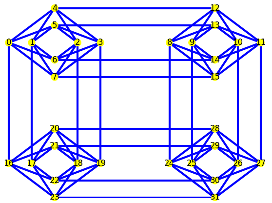
The length $r_{ij}$ of each connection is calculated from the diagram shown in Figure 1. This is a simplified model of the D-Wave architecture, not the actual physical layout of the quantum chip, here designed to show the effect of connectivity in spin networks. It is the general effect of differing coupling lengths that is being investigated here, rather than assigning these effects to particular qubits and connection lengths in the real hardware.

Algorithm 1 Pseudocode of algorithm used to generate the Hamiltonian matrix, M

1: NodeList                         ▹ list of nodes in the graph 2: EdgeList                            ▹ list of edges in graph 3: Positions                        ▹ list of x,y positions of nodes 4: Interaction                ▹ procedure returning $J_{ij}$, Equations (5)–(8) 5: remap NodeList, EdgeList, Positions from native nodes indices to indices used in Figure 1 6: M := zero $N\times N$ matrix                    ▹ Hamiltonian matrix 7: EdgeLength := list of Euclidean lengths of EdgeList edges, from Positions 8: $r_{min}$ := min(EdgeLength) 9: for idx = 1 to len(EdgeList) do 10:     $i,j$ := indices of nodes at each end of edge EdgeList[idx] 11:     $r_{ij}$ := EdgeLength[idx] 12:     $J_{ij}$ := Interaction($r_{min}$, $r_{ij}$) 13:     M[$i,j$] := M[$j,i$] := $J_{ij}$ 14: end for 15: return M

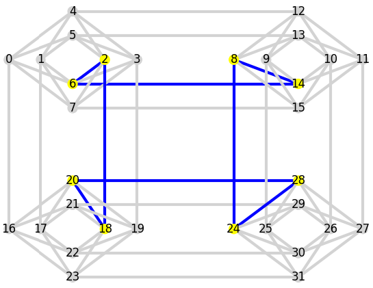
Throughout this paper, the qubit numbering shown in Figure 1 is used, even when only subsets of the qubits are simulated (Figure 3).

Once the Hamiltonian is generated, the simulator calculates the dynamics of the system as it evolves over time. At $s=0$, the system is initialised in the state $\left|\psi \right(0)\rangle$ with a single excitation across the network. Two different initial conditions are tested, both considering a single excitation. The first initial condition has the excitation localised in one qubit in the system: the state of that qubit is initialised to |1〉 with all others initialised to |0〉. The initial excitation is always in the qubit with the lowest index number in the particular network being simulated (for example, qubit #2 in the 8 qubit network of Figure 3). The second initial condition is an equal superposition of the excitation being localised at each of the sites within the network,

$$|\psi \left(0\right)\rangle =\left(\right|1,0,\dots 0\rangle +|0,1,\dots 0\rangle +|0,0,\dots 1\rangle )/\sqrt{N}.$$

(9)

In both cases, the excitation then propagates through the network according to the Hamiltonian $H_{xy}$ (given by Equation (4)).

The output of the simulator is the probability of the excitation being measured at each of the qubits at each of the time steps calculated. This excitation probability, often known as the fidelity, for qubit i is given by

$$F_i={\left|\langle 0_0{0}_1\dots 1_i\dots 0_N|\psi \left(s\right)\rangle \right|}^2$$

(10)

where $\left|\psi \right(s)\rangle$ is the state of the system at time s. Fidelity, being a probability, is dimensionless and restricted to the range $0\le F_i\le 1$ with ${\sum }_i^N{F}_i=1$.

To calculate these values, we solve Schrödinger’s equation following the method detailed in Mortimer et al. [28], which expands the system state in the eigenvectors of the Hamiltonian at each time step. The maximum simulation time used in each experiment is $t_{max}=10/J_{min}$. This was determined to be a physically relevant timescale over which an excitation could propagate through the network. Throughout this paper, the time steps are given as the dimensionless $t/t_{max}$.

4. Effects of Different Types of Qubit–Qubit Interactions

In this section, we consider a small network with eight qubits spread over four unit cells, as shown in Figure 3 (larger networks are examined in the following section). A subset of qubits of the full network are chosen to give all six possible different edge lengths $r_{ij}$ in the graph, to break the symmetry as much as possible.

Eight scenarios are simulated, one for each of the four interactions that govern the scaling of the coupling strengths in the network (constant, linear, Coulomb, dipole-dipole), for each of the two initial conditiosn (localised excitation, equal superposition).

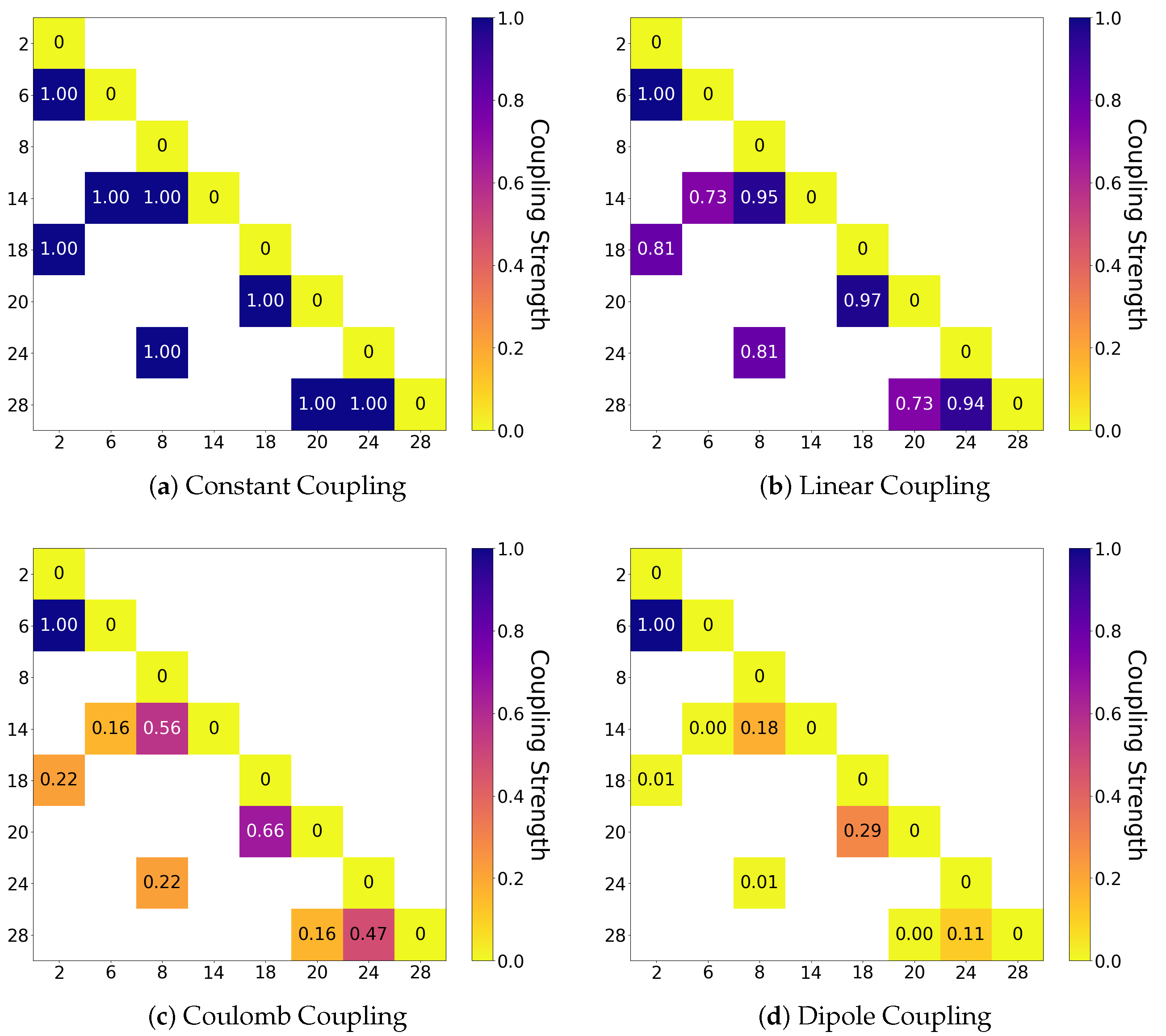
The simulation requires a set end-time, which we here define as $t_{max}=10/J_{min}$, where $J_{min}$ refers to the smallest coupling weight in the system. This time allows the excitation injected initially to spread across the whole network. This does mean that the total simulated time is different for each coupling scenario. The coupling weights for the 8 qubit network of Figure 3 are shown in

Table 1. Eight-qubit network: The six distinct coupling lengths $r_{ij}$ in normalised units of $r_{min}$ and corresponding coupling strengths $J_{ij}$ in normalised units of $J_{max}$, the strongest coupling, for each simulation scenario. The right-most column shows which connections in Figure 3 have each connection distance.

${\mathit{r}}_{\mathit{ij}}$	Constant	Linear	Coulomb	Dipole	$(\mathit{i},\mathit{j})$
1.000	1.000	1.000	1.000	1.000	(2,6)
1.518	1.000	0.970	0.659	0.286	(18,20)
1.777	1.000	0.955	0.563	0.178	(8,14)
2.112	1.000	0.936	0.473	0.106	(24,28)
4.592	1.000	0.807	0.218	0.010	(2,18),(8,24)
6.168	1.000	0.735	0.162	0.004	(6,14),(20,28)

and Figure 4.

4.1. Initial State with Localised Excitation

We first consider the case in which the initial state has a single excitation localised at the qubit of smallest index. The time evolution dynamics of these simulations across the defined time window are shown in Figure 5.

In the case of constant couplings, the length of the connection has no effect on the dynamics of the system. Therefore, the behaviours of the two qubits coupled to the initial excitation are expected to be identical. This can be seen in Figure 5a, where the lines denoting qubits (#6, #18) are exactly overlaid throughout the whole time window. In the same way, other qubit pairs behave identically based on the number of steps between the initial qubit #2 to the qubits in questions. These pairs are qubits (#14, #20), both a minimum two connections away from qubit #2, and qubits (#8, #28), both a minimum three connections away from qubit #2. Qubit #24 behaves unlike any other qubit in this network, being a minimum of 4 connections away from the initial excitation at qubit #2.

In the simulations with distance-dependent types of couplings, each qubit behaves differently because there is a different minimum distance between each qubit and the site of the initial injection, qubit #2. Hence, there are no overlaid lines on the dynamics’ plots. The number of oscillations increase from panels (a) to (d) within the same rescaled time. This is due to the increasing difference between $J_{min}$ and $J_{max}$. While $J_{max}$ is equal to one in all cases (because the lengths are rescaled such that the smallest is assigned $r=1$), $J_{min}$ becomes increasingly small as the effects of the differing connection lengths become more pronounced. When $J_{min}\ll 1$ (Coulomb and dipole couplings), the excitation is more strongly localised between qubits that are connected by the shorter couplings. This leads to high-frequency oscillations in excitation probability between qubits #2 and #6 (dark and light blue lines), and, to a lesser extent, between qubits #18 and #20 (red and pink lines). If these strongly coupled qubits were to be considered as ‘chained qubits’, their actual states during the dynamics are far from similar. This is further explored next.

4.1.1. Behaviour at First-Peak and Maximum-Peak Times

Results from simulations with distance-dependent types of couplings are more complex, so, to aid in their interpretation, we consider the dynamics at two specific timesteps within the simulated window of $0\le t\le t_{max}$: the time at which the first peak occurs after $t=0$, known as $t=t_{fP}$, and the time of the maximum peak within the time window (excluding the initial state at $t=0$), $t=t_{mP}$. The excitation probability of each qubit at these points are shown in Figure 6.

In the constant-interaction case, the maximum peak occurs at qubit #24, the qubit that behaves differently from any other due to it being the only qubit at its minimum number of connections from the initial excitation. This causes the highest peak excitation probability because both routes to this qubit (approximately clockwise and anticlockwise) have the same number of steps, and so the components of the initial excitation interact constructively at that site. In this simulation, distances between adjacent qubits are accounted for by the couplings’ strengths, so if these strengths are constant, it is as if the distance between adjacent qubits is always the same.

In the linear-interaction case, the maximum peak occurs at qubit #8, which at first appears counter-intuitive because it is a minimum of three hops away from the initial injection site. However, the path to each qubit can be made up of any number of clockwise and anticlockwise steps, and it is non-trivial to trace back the source of excitation probability at any particular time.

This complicated behaviour is seen even more explicitly in the case with dipole-dipole couplings. In this case, the coupling strengths of the longest and shortest edges are 0.004 and 1, respectively (Table 1). With this disparity, it is expected that the excitation probability is localised for an extended period of time to just traversing the short connection between qubits #2 and #6. Indeed, this is seen in both Figure 5d and Figure 6g,h.

4.1.2. Similarity Indicator

In addition to considering the overall dynamics, we also compare the fidelities of all connected qubits within the network at $t_{fP}$ and $t_{mP}$. We define a similarity indicator, ${\Delta }_F$, for each edge as follows:

$${\Delta }_F=|F_i-F_j|$$

(11)

where $F_i$ and $F_j$ represent the excitation probabilities of qubits i and j, respectively (as given by Equation (10)). When an edge has ${\Delta }_F=0$, the qubits at each end of the edge have the same excitation probability. For strongly interacting chained qubits, ${\Delta }_F=0$ would be expected at all times.

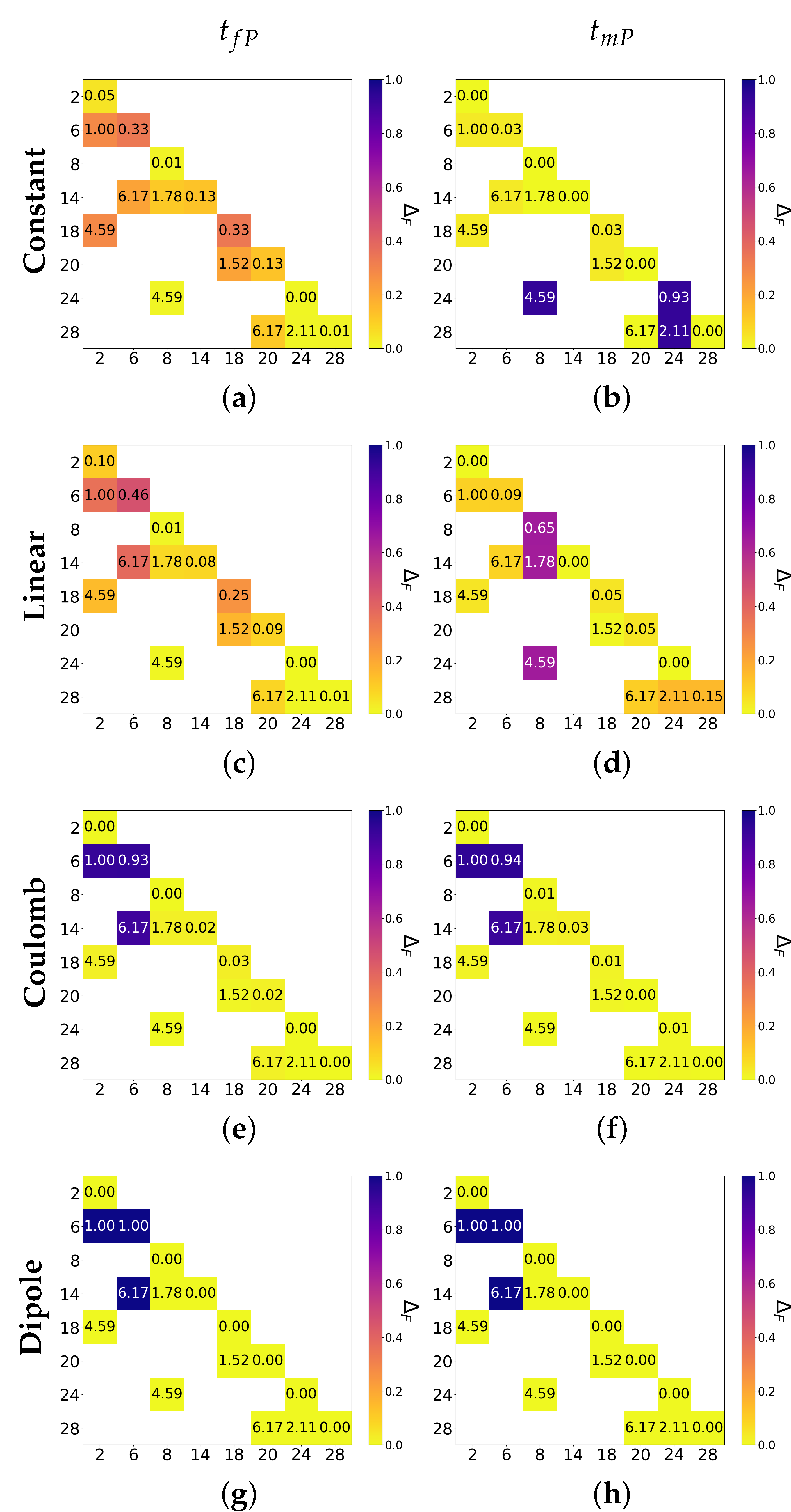
The ${\Delta }_F$ values for the edges in this network are shown in Figure 7, where each off-diagonal square represents the edge connecting the qubits labelled at its x and y positions. The squares in these plots are colourised by the ${\Delta }_F$ value and are labelled with the normalised lengths of each edge. The squares on the diagonal are coloured and labelled with their excitation probability at that time step; this is a repeat visual of the data shown in Figure 6.

When the coupling between qubits is constant, we would expect the length of the connection to have no effect on the similarity between the qubits (i.e., both non-zero squares in any given row should have the same similarity). This is true in the first column of both of the first and max peak charts in Figure 7, but is not the case beyond the second column. We suggest that this is because of the cyclical connectivity of the network and the lack of directionality in the connections. The lack of directionality comes from the fact that qubit interactions are symmetric. The excitation can propagate on a number of different routes from one qubit to any other, so the excitation probability resulting on each qubit is not simply a result of the qubits it is directly connected to, but of all the qubits in the network and the topology of their connectivity.

In the Coulomb and dipole–dipole cases, we should expect that the smallest connecting edge to give rise to a higher similarity (a low ${\Delta }_F$) between the qubits, shown as an orange/yellow square. This is not the case at either of the time steps chosen for analysis here: see square $(2,6)$ in Figure 7e–h. So this would not support the use of chaining in these cases. The similarities in each case are different from that in the control case of constant coupling, which means that the different physical interactions do have an effect on the similarity measured between connected qubits (also seen in the dynamics shown in Figure 5). It appears from these results that the connectivity of the network has a larger impact on the correlations between the qubits than does the edge lengths and corresponding coupling strengths: even in the constant coupling case, the similarity between qubits appears affected by more than just the immediate neighbours. This is further examined in the next section, with alternative larger networks.

4.2. Equal Superposition Initialisation

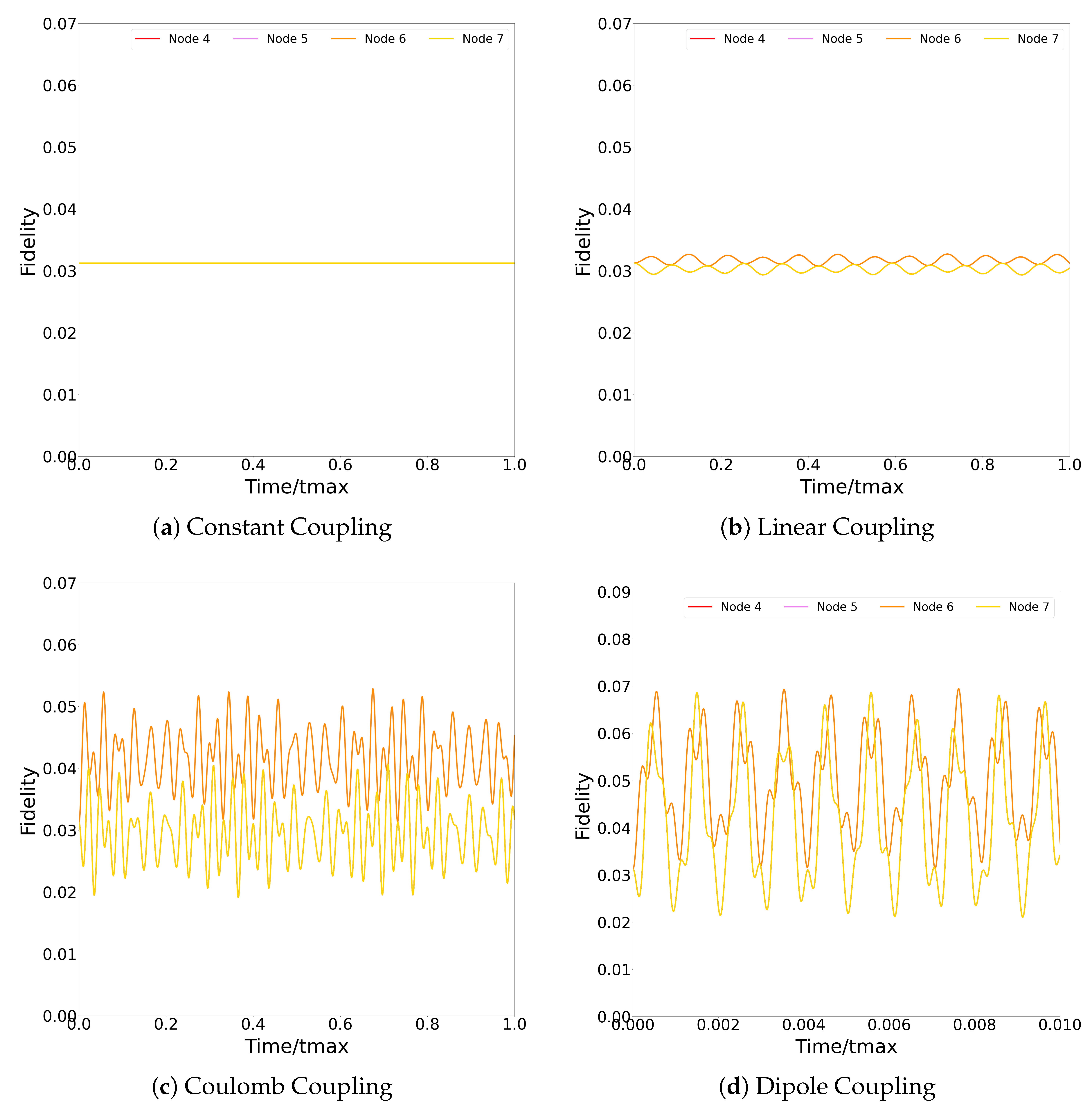
Figure 8 shows the dynamics of the eight-qubit network when initialised in the equal superposition state Equation (9). In this network, the qubits and edges form a single loop, Figure 3. In the single-excitation case, the Hamiltonian has eight eigenstates. When all the couplings are constant, one of the eigenstates is the equal superposition state Equation (9), which is why no dynamics are seen in Figure 8a.

When the coupling strengths are then related to the lengths of the edges in the diagram (by Coulomb, linear, or dipole–dipole interactions), a different Hamiltonian is produced and the equal superposition state is no longer an eigenstate. This results in the dynamics seen in the graphs.

For the strongest dependence of the coupling strength on the coupling length (dipole-dipole coupling, compare columns in Table 1), pairs of qubits connected by shorter links excite in phase and to a similar strength. However, in the intermediate cases, the excitation probability of nearby qubits may oscillate out of phase (all cases in Figure 8b and the pair of qubits #24 and #28 in Figure 8c) or show opposite trend with respect to the average occupation probability (pair of qubits #18 and #20 in Figure 8b).

In D-Wave devices, chains of qubits are constructed to emulate otherwise unavailable connectivity in the network. To achieve this effectively, qubits in the chain should behave identically. In our simulation, this is when the qubits excite in phase. In the linear case, the qubits connected by the shortest lengths appear out of phase with each other. In the Coulomb case, they are much closer in phase, and in the dipole–dipole case they are visually in phase. This suggests that to use chaining effectively, one would want to be in a dipole–dipole coupling regime.

4.3. Implications on Chaining

The initialisation states tested here have different implications for the use of chaining in qubit networks. As previously mentioned, chaining is used to artificially improve the connectivity of a single logical qubit by having multiple physical qubits behave as one. This is typically implemented by having strong coupling strengths between the physical qubits to ensure that they behave identically. We showed that this is not necessarily the result of strongly coupled qubits.

In the localised single excitation initial state, when the coupling between qubits is strong, their respective fidelities vary greatly throughout the time window. In the case of an equal superposition initial state, strongly coupled qubits excite in phase, making this an effective regime in which one could implement chaining. Thus far, these results are qualitative and suggest that both the initial conditions and the coupling regime have significant impact on the potential use of chaining in real computational systems. Further analysis is required to quantify the phase difference in the dynamics of two or more strongly coupled qubits in a variety of regimes. How strongly and in what configuration the chain connects to the rest of the network is likely to be an important consideration.

5. Analysis of Connectivity Effects

In this section, we use the simulator to test how a larger 32-qubit network (Figure 9) performs compared to the 8-qubit network of the previous section. This size of simulation was chosen because it now uses all the possible qubits and connections in the $2\times 2$ unit cell of Chimera architecture as present in a full D-Wave 2000Q chip (which has 2048 qubits). Any larger network simulations are prohibitively expensive in terms of computation time and power when required to calculate all qubit fidelities at every time step in the simulation.

Due to the design of the initial eight-qubit network, this larger network has the same six different coupling lengths (Table 1), with multiple connections having the same lengths.

This network is used with the simulator to produce dynamics for each of the initial state and coupling scenario combinations. The fidelities at the times of the first and maximum peaks are calculated using the same methodology as in the eight-qubit case.

5.1. Localised Excitation Initialisation

The excitation probability results for the 32-qubit network given a localised excitation initial state are shown in Figure 10. The excitation is inserted in qubit #0.

In these 32-qubit plots, the scale of the fidelities is different from that of the previous plots. The larger number of qubits means that the excitation probability is generally much more distributed through the network; the scale used in Figure 7 would make it difficult to see the difference between the qubits here. In the 32-qubit case, unlike the 8-qubit case, the occupation probability is generally much less concentrated on single qubits. We suggest that this is because there are now a number of different ’sub-loops’ within the network, increasing the number of possible paths that an excitation could propagate along to traverse the network.

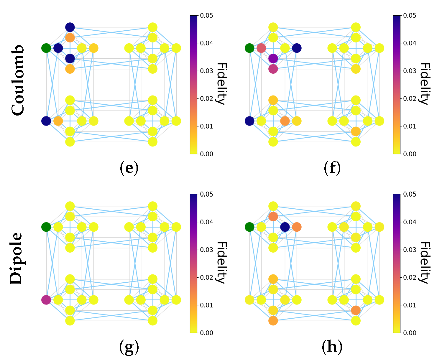
Dipole–dipole coupling at first peak (Figure 7g) shows non-zero fidelities only in the first unit cell, reflecting the short connections effectively confining the excitation with much stronger couplings as compared to the longer inter-cell connections. From the fidelities shown here, we know that the majority of the excitation probability remains on the initial qubit.

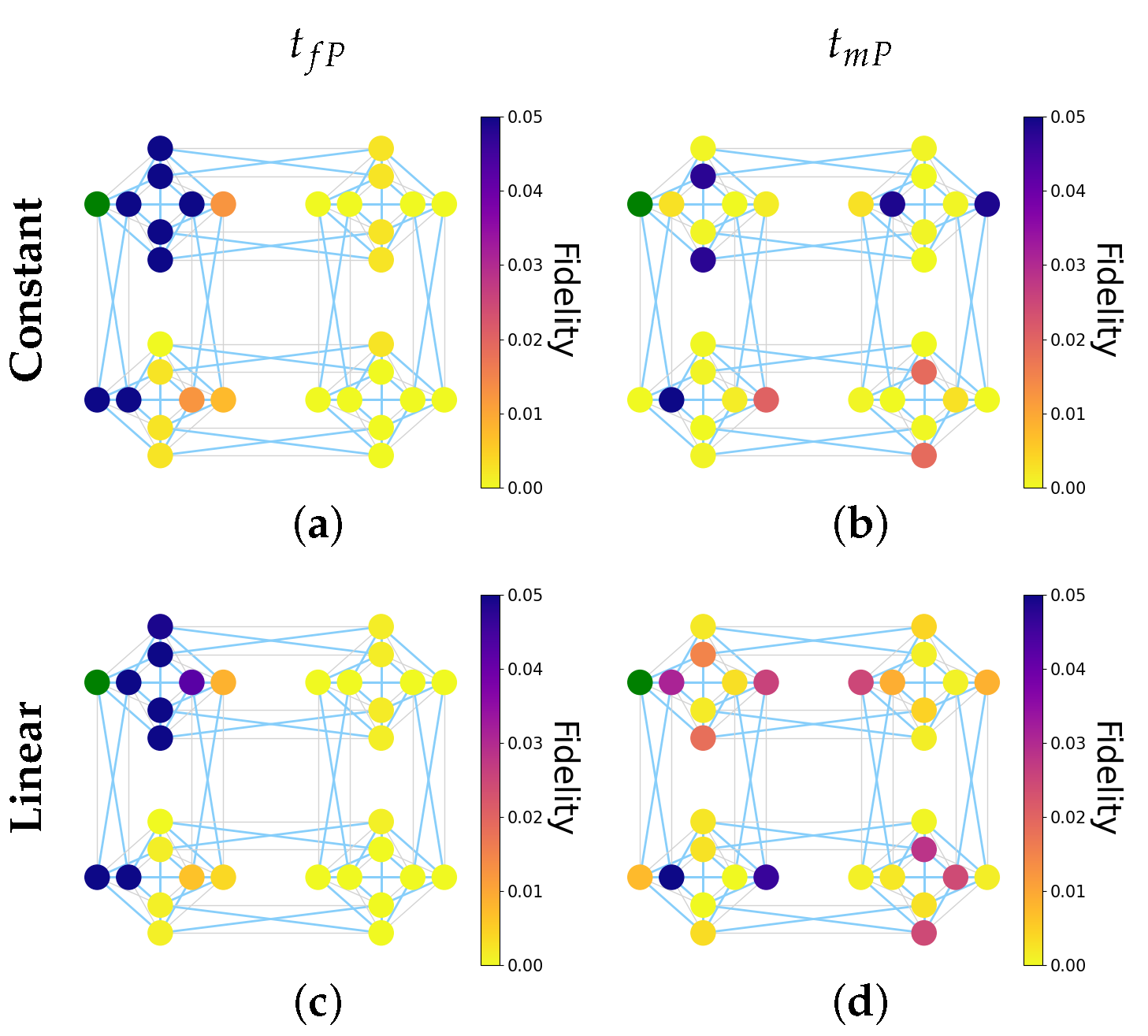
What is apparent in all the coupling scenarios of the 32-qubit network is the emergence of horizontal and vertical lines of similarly coloured qubits in the $t=t_{mP}$ graphs (banding). These are seen most clearly in the constant and linear cases and less so with the Coulomb and dipole–dipole interactions. In each unit cell of the constant coupling case (Figure 7b), either the four qubits in a horizontal line are orange and the vertical line is yellow, or vice versa. We note the similarity of our results to those seen by Nelson et al. [11], which includes a single qubit fidelity assessment of the qubits in a D-Wave 2000-Q quantum annealer chip (which has the Chimera architecture considered here). Nelson et al. show that horizontal and vertical qubits systematically respond differently to stimuli and suggest a number of possible causes, including issues with the delivery of the control signals and potential heterogeneity in the qubits. In our simulation, there are no control signals to consider as we are calculating just the time evolution of the system, and there is no inherent heterogeneity as all the qubits are simulated in the same way. Our results suggest that banding is a feature of the network layout itself, although the external stimulus is different in our case from that in [11]. Although there are a number of published works on the effects of errors in a quantum annealer in terms of its problem solving capability, as far as the authors here are aware, the work completed by Nelson et al. is the only published work looking at the response of individual annealing qubits to stimuli. The dataset produced in that study is the only comparable dataset available for this work.

In practice, a D-Wave quantum annealer can be regularly re-calibrated to tune the control lines in order to negate unwanted effects in the qubits and couplers [24]. Ideally, the length of the couplings should have no effect on the programmed coupling strength to allow a Hamiltonian such as Equation (1) to be executed as accurately as possible. Calibration, therefore, is used to ensure the couplings perform as closely as possible to this case. The fact that the horizontal and vertical bandings are seen both in the real chip in [11] and most prominently in the constant coupling case simulated here suggests that the calibration is mostly successful.

The linear coupling case shows some of this banding effect, though slightly diminished, because the inhomogeneity of the unwanted interactions is small compared to the reference constant couplings. As the effects of the inhomogeneous couplings become dominant (as in the Coulomb and dipole–dipole cases), these vertical and horizontal correlations disappear altogether.

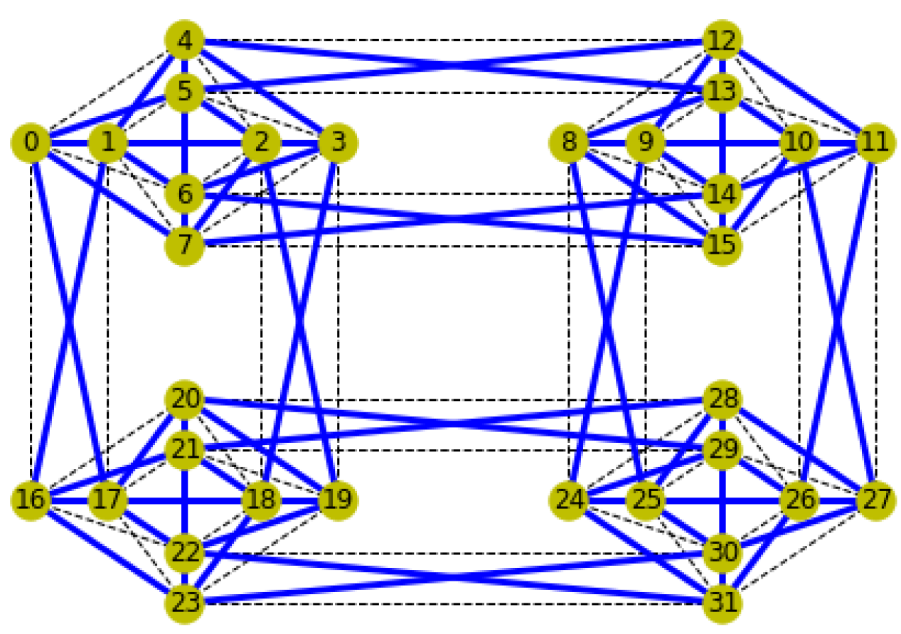
We speculate at this stage that having homogeneous coupling strengths is not the sole factor in causing these banding patterns, and suggest that the highly symmetric nature of the graph is also likely to cause these lines of similarly behaving qubits. In order to test this idea, we design a bespoke architecture with less symmetry and perform the same simulator experiments. The results are given in Section 6.

5.2. Equal Superposition Initialisation

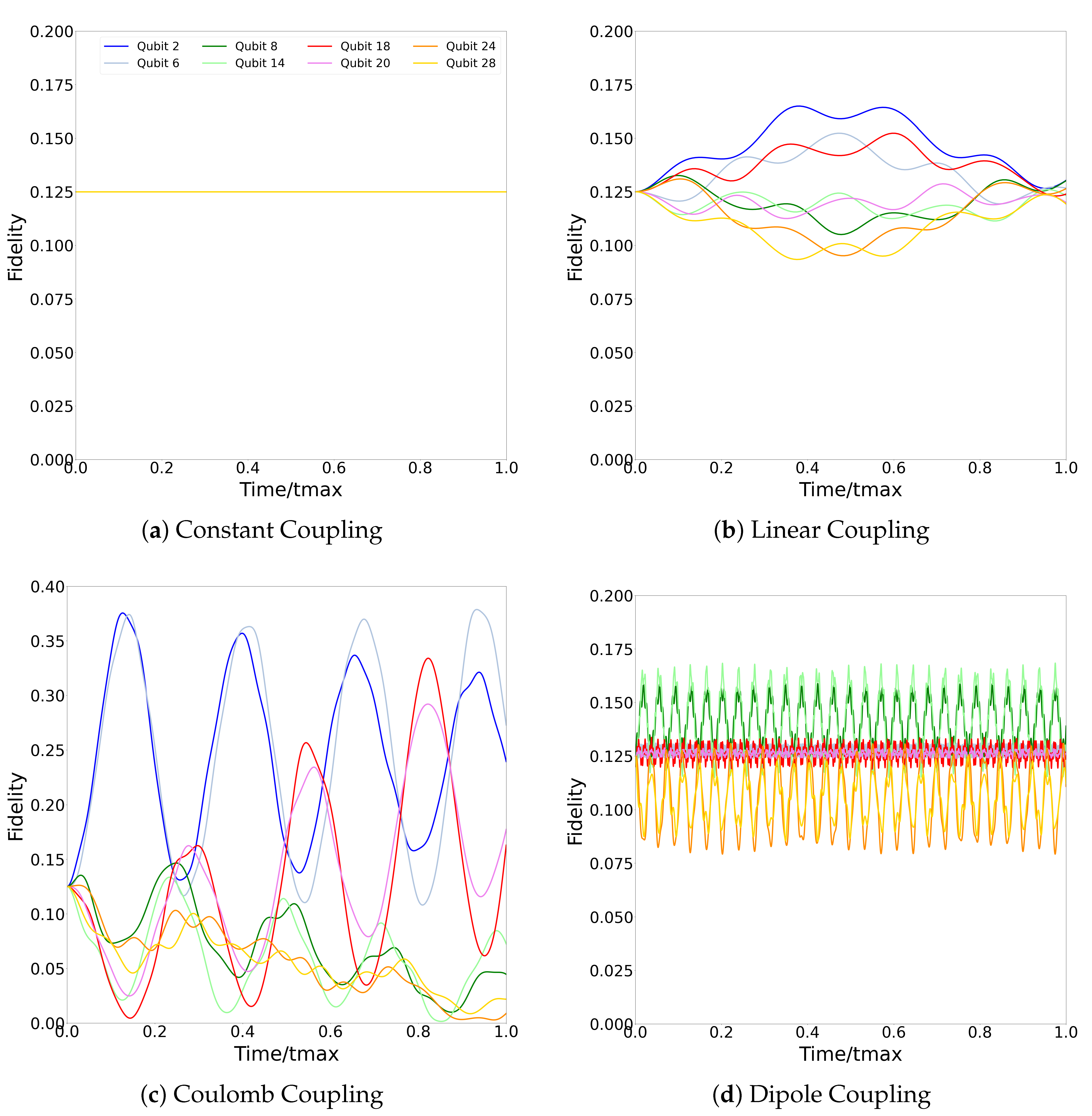
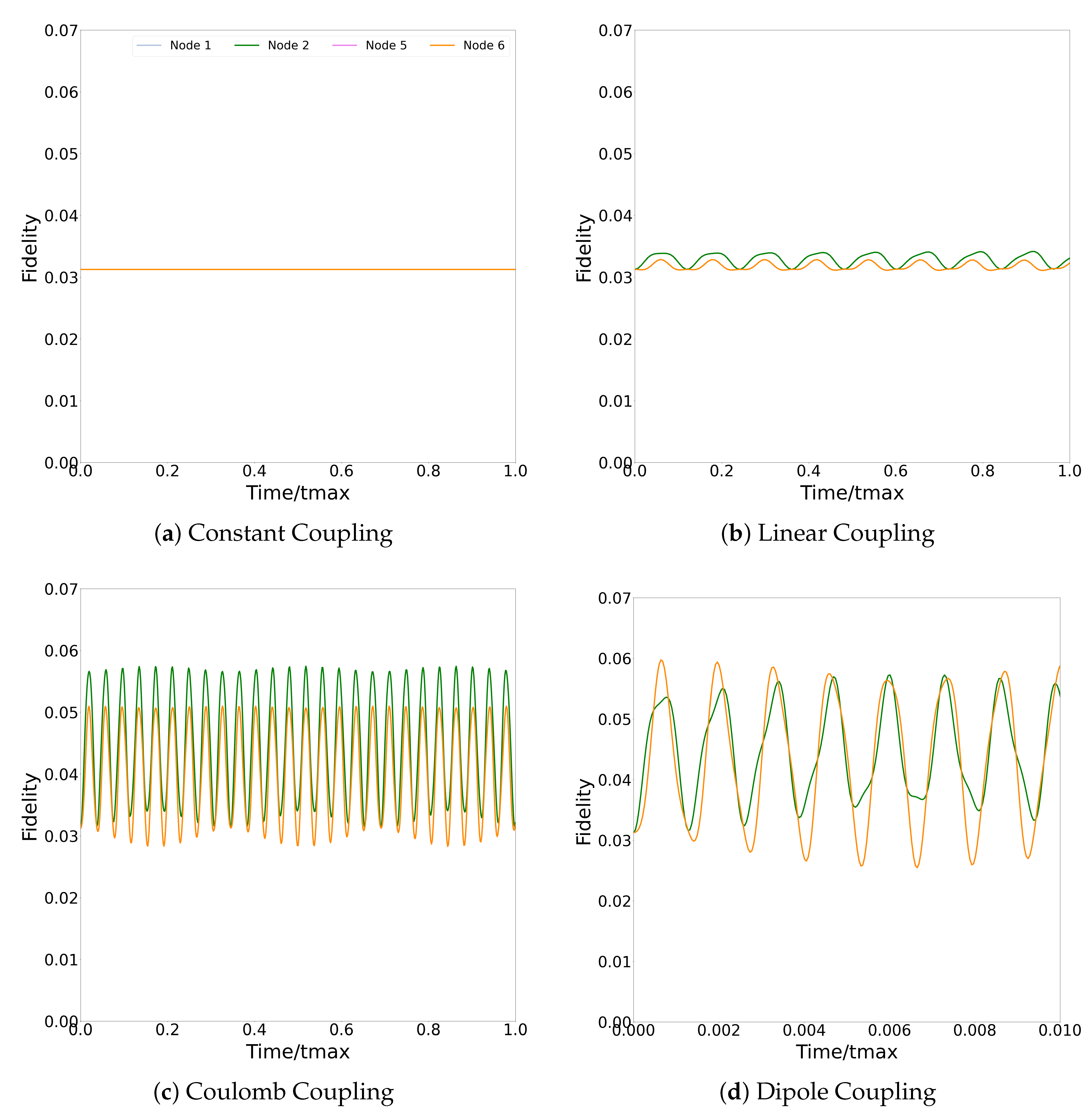
As in the 8-qubit network, the equal superposition state of the 32-qubit network shows no dynamics in the constant coupling case. Numerical analysis shows that in the 8-qubit case, this is due to the state being an eigenstate of the Hamiltonian, and the same is true here. Dynamics are seen in the other coupling scenarios reflecting that the equal superposition state is not an eigenstate of those Hamiltonians. In the eight-qubit case, linear coupling caused nodes linked by the shortest connections to be out of phase and dipole–dipole coupling caused these qubits to be in phase. In this case, the shortest connections are between qubits $(1,5),(1,6),(2,5),(2,6)$. Figure 11 shows the dynamics of these four qubits in the shortest connections in the top left unit cell of the network throughout the time window. In all cases, qubit #1 is exactly overlaid with qubit #2 and qubit #5 is exactly overlaid with qubit #6. This can be explained by the symmetric position of these qubits with respect to the centre of the cell. In all cases with dynamics, the qubits connected by short connections are approximately, but not exactly, in phase. Even for dipole–dipole coupling, this is combined with significantly different peak fidelities.

For the three cases in which there are dynamics in the system after an equal superposition initialisation, we plot the occupation probabilities of the qubits at the time of the maximum peak in the system, Figure 12. When the initial excitation is localised on one qubit (Figure 10), this shows horizontal and vertical banding; here, in the case of an equal superposition initialisation, it instead appears to create clusters of qubits with similar fidelities (Figure 12). The clusters of qubits with similarly high fidelities (those in purple) are connected in a ring of relatively short connections. This effect is most prominent when the coupling strength is highly dependent on the connection length (the dipole–dipole case) but is washed out by coupling strength weakly dependent on distance (linear case). This effect could be appropriate for use in chaining within D-Wave machines, provided that coupling strengths are strongly dependent on qubit distance. We caution, however, that, as noted in Figure 11, peak occupation value may be significantly different even for strongly coupled qubits, and relative phase differences from the fidelities’ oscillations may occur even for dynamics generated by strongly delocalised states.

6. Bespoke Architecture

To investigate whether the particular coupling layout seen in the Chimera architecture gives rise to the horizontal and vertical bandings seen in Figure 10, we designed a bespoke architecture based on the qubit positions of the Chimera graph but with different couplings and a larger variety of connection lengths. It would not be possible to implement this bespoke network on a real D-Wave chip with the Chimera architecture (without the use of embedding algorithms and ancilla qubits, thereby further distorting the reults).

The bespoke network is shown in Figure 13; the connection lengths and calculated coupling strength are given in

Table 2. Scaled connection distances and calculated coupling strengths for each simulation scenario in the bespoke network architecture of Figure 13. The right-most column shows an example coupling of that length. Other lengths can be determined via symmetry.

Distance	Constant	Linear	Coulomb	Dipole	$(\mathit{i},\mathit{j})$
1.000	1.000	1.000	1.000	1.000	(4,5)
1.325	1.000	0.987	0.755	0.430	(0,1)
1.492	1.000	0.981	0.670	0.301	(1,6)
1.900	1.000	0.965	0.526	0.146	(5,6)
2.264	1.000	0.951	0.442	0.086	(1,4)
2.300	1.000	0.949	0.435	0.082	(1,2)
2.651	1.000	0.936	0.377	0.054	(0,5)
3.151	1.000	0.918	0.317	0.032	(0,7)
3.900	1.000	0.890	0.256	0.017	(4,7)
4.950	1.000	0.854	0.202	0.008	(0,3)
6.977	1.000	0.787	0.143	0.003	(0,17)
9.254	1.000	0.719	0.108	0.001	(4,13)

. The pattern of connections follow the same structure of the original Chimera graphs: each qubit is connected to four other qubits within its own unit cell and one in a neighbouring unit cell.

It was decided to not increase the number of qubits in the bespoke networks for a number of reasons: the first being the computation time required for simulation (as discussed in Section 5), the second being to perform a direct comparison with the standard 32-qubit network and the third being that the dynamics seen in a 32-qubit network are already very complex and increasing the size of simulation would further increase the difficultly of analysing and disentangling the effects seen in the results.

6.1. Localised Excitation Initialisation

The excitation probability results from the simulation of the bespoke architecture under a localised excitation initial state are shown in Figure 14. In this case, the $t=t_{mP}$ graphs do not show the same horizontal and vertical banding seen in the 32-qubit Chimera graph. Where we saw the banding patterns in the previous network, the swapped connections that link different unit cells appear to have induced an alternating pattern of qubits with low and high excitation probability in some of the unit cells. These results help to confirm the conclusion from the previous section that it is the connections between the qubits that cause the banding of horizontal and vertical qubits seen in both our Chimera architecture simulation and in [11]. However, there is some evidence of a pattern in this bespoke network as well, which suggests that in any architecture with repeated unit cells and formulaic connections between the qubits there would be a distinctive patterning of the fidelities at peak times.

6.2. Equal Superposition Initialisation

Although the connections are different from those of the true Chimera architecture, when the system is initialised in the equal superposition state, there continues to be no dynamics in the constant coupling case, from which we can infer that the state is also an eigenstate of this Hamiltonian. When the couplings are constant (and therefore unrelated to length), the only difference between this network and the Chimera one in Section 5 is the numbering. Since we retained the overall structure of the previous network by ensuring that each qubit is connected to four within the unit cell and one from a neighbouring cell, all that has changed between these networks is in relation to the locations of the qubits that are connected. Unlike in the real hardware, qubits are now connected to those with the same orientation rather than all internal connections going to qubits of opposing orientation.

Figure 15 shows the four qubits in the top left unit cell that are connected by the shortest connection: $(4,5)$ and $(6,7)$. In all coupling scenarios, node #4 is exactly overlaid with node #6 and #5 is exactly overlaid with #7. The occupation probability of the nodes at either end of this very short coupling are approximately anti-phased in the linear case. As the coupling strength dependence on the coupling length increases, the situation is less clear cut. A difference with the Chimera network is that the difference in length between the two shortest lengths here is not high enough to decouple the corresponding beating frequencies (compare the first two lines of Table 1 and Table 2). As a result, some of the occupation peaks are in phase and some are out of phase depending on how the beating affects each of the strongly coupled nodes. With respect to chaining, this result cautions on the interplay between beating from different, but close, coupling lengths, even in the case of a very strong dependence of coupling strength on coupling length.

In Figure 16, showing the qubit fidelities of $t_{mP}$, neither the alternating pattern seen in Figure 14 nor the clustering seen in Figure 12 are well defined. It could be that a mixture of the two effects is being seen, with the graph structure causing some alternating fidelities in the clustering structure caused by the equal initial state. This is an example of how even simple networks and initial conditions can induce complicated effects. It highlights the need to perform experiments in tightly controlled simulations before trying to relate the results to real quantum devices; the latter may further be affected by inhomogeneity, noise, and other potential error sources.

7. Effects of Noise

Thus far, the simulations have been exclusive of any noise in the system. This is helpful for understanding the ideal system dynamics of these networks. However, noise can arise from difficulty in controlling the environment around the qubits, and from errors induced in the fabrication process preventing the qubits and couplers from being identical. These types of noise can be modelled simply as a Gaussian perturbation on the coupling strengths of the network.

Here, we model a $1\%$ and a $5\%$ noise (relative to the average $\overline{J}$ of the non-zero couplings $J_{ij}$ in the system) by adding to each non-zero coupling a random perturbation generated from a Gaussian distribution with a mean equal to the average coupling in the noiseless scenario $\overline{J}$ and a standard deviation of 0.01 or 0.05, respectively. The dynamics are calculated in the same way as in the previous sections.

Most quantum computing platforms quote qubit error rates less than $1\%$, so this is a realistic scenario with $5\%$ being an extreme worst case. For each scenario, 1000 Hamiltonian matrices with the structure of the eight-qubit network, but with randomly sampled noise, are generated. The dynamics are calculated for the two points in time analysed in the previous sections: the time of the first peak and the time of the maximum peak. These times are taken from the noiseless scenario and the state of the noisy systems at these times is then calculated directly.

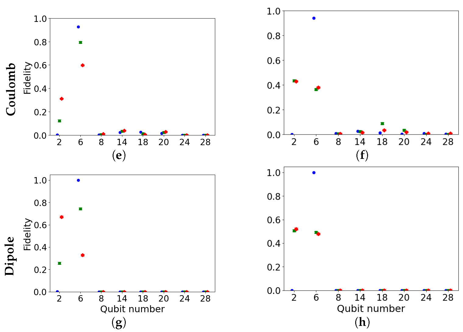
The results of these simulations are shown in Figure 17. In individual samples, the qubit fidelities can vary from the mean; averaged across the many samples, the noiseless scenario is largely recovered.

At the time of the first peak, there is a shift in weight between qubits as the imperfections are increased. The total fidelity of all the qubits has to add to one (this is not exact for the average, but since the variance on the mean is very small, this can largely be assumed), so if the fidelity in one qubit goes up, it has to go down in other qubits. This shifting is likely to be between directly connected nodes. As time progresses, the effects of the noise increase due to the increased number of couplings affecting the spreading of the excitation through the network and the diverging of the evolution of the deformed wave function from the ideal one. By the time of the maximum peak there is a much larger deviation from the noiseless scenario. These deviations differ from sample to sample, but averaged across all the simulations, it has the effect of moving the qubit fidelities towards a more even distribution.

Figure 17e–h show the noisy simulations of the two coupling graphs with the most length dependent couplings. Both the first and max peak graphs look similar. In the noiseless dynamics (Figure 5d), the frequency of the beating between Qubits 2 and 6 is very high; the oscillations happen so fast that when noise disruption is added, in approximately half the cases, the peak is on the opposite qubit. When averaged over many runs, this gives the fidelity around 0.5 with a very large spread. Figure 18 demonstrates this effect by showing large peaks around 0 and 1 for the occupation probability of Qubit 2.

8. Conclusions and Future Work

This work used a number of different simulations to demonstrate the effect that both connectivity and physical interactions between qubits can have on the dynamics in a network of spins. We showed that, even with small tightly controlled networks, complex behaviour appears due to the interconnected nature of the qubits allowing multiple possible paths for an excitation though the network.

In the cases with simulated Coulomb or dipole–dipole interactions, we expected that a shorter edge length would result in similar excitation fidelities between the qubits. This was not found to be the case, which we suggest is a result of the complex connectivity having a greater effect on the dynamics than changing the coupling interaction between the qubits.

To further investigate this result, we simulated a larger network of 32 qubits in the same way. When coupling strength is related to length, at times early in the simulation, we see that there is higher excitation probability for qubits in the unit cell in which the excitation was inserted at $t=0$. This is to be expected as connections internal to the unit cell are shorter than those between unit cells. However, this is not the case at later times, suggesting that the complex connectivity has more of an effect as time progresses. This is interesting when considering that this architecture is used on the D-Wave 2000Q quantum annealing chip. For effective annealing, one wants to anneal as slowly as possible to have the most chance of resulting in a ground state of the system whilst not allowing decoherence of the qubits. Long time scales also reduce the effect of the unwanted couplings between qubits in relation to the effects caused by the connectivity as excitations are often confined to regions in shorter timespans. Not having to balance these factors is likely to increase the success probability of quantum annealing.

At the time of the maximum excitation peak within the simulated time window, there are horizontal and vertical bandings that appear in the fidelities of the qubits when the coupling strength is either constant or close to constant (linear coupling regime). This is similar to the correlations seen in [11] that completed a single qubit fidelity assessment on the qubits in a D-Wave 2000Q chip with the same architecture as the simulated networks tested here. This suggests that the real chip is likely subject to constant or close to constant coupling strengths, which is the desired situation for quantum annealing. This is likely due to the calibration that is performed on the chip, which tunes the control lines to account for any unwanted interactions between the qubits.

We hypothesised that these bandings are likely a result of the particular connectivity in the Chimera architecture; to provide evidence for this, we designed a bespoke network for simulation in which the qubits are in the same positions as before but the connections are changed. Indeed, no linear banding is seen in any of the results for the simulations run over this network. In fact, a different pattern is seen, in which the fidelities of neighbouring qubits appear to oppose each other in a number of cases. We conclude that any particular architecture is likely to introduce its own reproducible patterns in the fidelities of its qubits given a long enough window of time evolution. To extend the study on the bespoke network, it would be an interesting avenue of future work to run the simulation over a network with qubits in the same relative locations but with completely random connections (perhaps only stipulating an average of five connections per qubit). This would likely eliminate any repeating structure in the network and resulting simulation results.

These experiments showed mixed results in regards to the use of chaining in D-Wave networks. When the network is initialised with a single excitation, strongly connected qubits oscillate out of phase which would not be effective for implementing chaining. However, when the network is initialised with an equal superposition state, the qubits connected by strong couplings show fidelities that operate in phase. This regime wold be appropriate for chaining. Understanding how physical errors manifest in real D-Wave devices would then show how these errors might affect chaining.

Simulating the effects of Gaussian noise on the simulations show that for realistic levels of noise (such as that caused by environmental or manufacturing inconsistencies), the conclusions from the noiseless simulations still hold. When the noise level is increased, the simulations shows a tendency to move towards an equal superposition of fidelities as time progresses.

Next steps should include running similar experiments on a real D-Wave chip to demonstrate the link between the simulations shown here and the practical performance of a quantum annealing chip. To produce similar time dynamics from a real chip requires a large number of samples from the system at each time step. Sampling problems are commonly solved on quantum annealing chips, so a similar methodology could be followed [29,30,31]. In order to achieve this most efficiently, small networks could be set up to run in parallel on a single chip (assuming relative isolation between the networks) [32].

It would also be beneficial to use these simulations in conjunction with real devices in order to better characterise the calibration and control pulses that are used to improve performance in practice. Typically, calibration and control are expensive tasks in terms of both time and complexity, and a better understanding of the effects could help make these processes more efficient or be required less frequently [33].