Abstract
Accurately predicting the ionosphere’s Total Electron Content (TEC) is significant for ensuring the regular operation of satellite navigation and communication systems and space weather prediction. To further improve the accuracy of TEC prediction, this paper proposes a TEC prediction model based on the grid-optimized Gate Recurrent Unit (GRU). This model has the following main features: (1) it uses statistical learning methods to interpolate the missing data of TEC observations; (2) it constructs a sliding time window by using the multi-dimensional time series features of two types of solar activity indices to support modeling; (3) It adopts grid search combined with optimization of network depth, time step length, and other hyperparameters to significantly enhance the model’s ability to extract the characteristics of the ionospheric 11-year cycle and seasonal variations. Taking the EGLIN station as an example, the proposed model is verified. The experimental results show that the root mean square error of the GRU model during the period from 2019 to 2020 was 0.78 TECU, which was significantly lower than those of the CCIR, URSI, and statistical machine learning models. Compared with the other three models, the RMSE error of the GRU model was reduced by 72.73%, 72.64%, and 57.38%, respectively. The above research verifies the advantages of the proposed model in predicting TEC and provides a new idea for ionospheric modeling.
1. Introduction
The ionosphere is a plasma-rich region containing substantial ions and free electrons, spanning approximately 60 km above the Earth’s surface to the top of the magnetosphere. As a critical medium influencing satellite–ground electromagnetic-wave propagation, it induces signal delays, attenuation, and scattering in radio communication and navigation systems [1].
TEC represents the cumulative electron density along a signal transmission path. It serves as a key parameter for measuring the spatial and temporal inhomogeneities and disturbance characteristics of the ionosphere, as well as the signal delay [2]. TEC can be directly measured using observed instruments [3]. Current satellite-based TEC retrieval methods exhibit an inherent latency of several hours. Therefore, ionospheric modeling is essential to enable near-real-time TEC estimation, thereby enhancing the timeliness of space environment monitoring [4]. High-precision ionospheric models effectively mitigate ionospheric effects in signal propagation [5], providing error compensation solutions for satellite–ground wireless communication systems and advancing the understanding of coupling mechanisms between solar activity and geospace environments.
Given the complexity of ionospheric dynamics, diverse modeling approaches have been developed in academia. The International Reference Ionosphere (IRI) model has emerged as the international standard for predicting ionospheric parameters, garnering significant scientific attention [6,7]. The IRI model integrates multi-source data, including solar activity indices and geomagnetic parameters, and generates predictions for quiet-time critical frequencies, altitude information, and TEC values. Jointly developed through international scientific collaboration and subject to continuous refinement, the IRI has evolved over a dozen iterations, spanning versions from IRI-78 to IRI-2020 [8,9]. Researchers worldwide have developed numerous regionally corrected models within the IRI framework to enhance regional applicability. These observation-driven empirical models, characterized by structural simplicity and computational efficiency, are widely employed for ionospheric TEC prediction.
In recent years, with the development of intelligent algorithms, machine learning has significantly advanced the innovation of ionospheric modeling. Researchers have introduced nonlinear methods such as Artificial Neural Networks (ANNs) and empirical orthogonal functions into predicting and analyzing parameters, such as TEC, critical frequency of the ionospheric F2 layer (foF2), and peak height. Some of these achievements have been incorporated into the international standard system. Typical achievements include the following: Liu et al. [10] established a European regional prediction model by introducing statistical machine learning; Jia et al. [11] proposed an improved radial basis function neural network classification method by integrating partial least squares and genetic algorithms; Hu et al. [12] enhanced the prediction accuracy of foF2 by using the particle swarm optimization algorithm to improve the backpropagation neural network; Zhang et al. [13] employed an encoder–decoder structure combined with convolutional optimization to the long short-term memory network to achieve the prediction of TEC; Wang et al. [14] developed a global ionospheric model based on an ANN optimized by genetic algorithms; Weng et al. [15] innovatively combined adaptive genetic algorithms with BP networks to construct a combined prediction model; Xia et al. [16] utilized GPU-accelerated support vector machines to achieve hourly step TEC prediction; and Yu et al. [17] established a long-term TEC prediction model using a support vector regression model. These studies have effectively improved the prediction accuracy of ionospheric parameters through algorithm innovation or data fusion.
While these methods demonstrate notable advancements, they exhibit inherent limitations for capturing long-term ionospheric dependencies: ANN and BP architectures often face challenges in modeling extended temporal sequences due to gradient vanishing issues; SVR models, despite their robustness, scale poorly with high-dimensional solar-terrestrial datasets; and LSTM networks, though effective for temporal patterns, incur substantial computational overhead from their complex gating mechanisms. In contrast, the Gated Recurrent Unit (GRU) provides a balanced solution—preserving LSTM’s capacity for long-range dependency modeling while reducing parameter complexity and training latency through its streamlined dual-gate design—making it particularly suited for TEC sequences governed by decadal solar cycles and seasonal variations.
To further enhance the accuracy for predicting the long-term variation characteristics of TEC, this paper proposes a prediction model based on grid-optimized gated recurrent units. It combines a data filling strategy to optimize the modeling process. The structure of this paper is as follows: Section 2 provides an introduction to GRU and grid optimization methods; Section 3 introduces the ionospheric TEC data and solar activity index data used in this paper; Section 4 conducts data preprocessing and applies a GRU for modeling to complete the training of the model; Section 5 compares the established GRU model with the IRI model and Statistical Machine Learning (SML) model to complete the testing of the GRU model; and Section 6 summarizes this paper.
2. Methodology
This section systematically elaborates on the core mechanism of the model design from a theoretical perspective. The GRU models the dependency of time series data through gating dynamics. At the same time, the grid search method achieves joint optimization of hyperparameters based on the global traversal property of the parameter space. Combining these two methods provides an approach for ionospheric TEC prediction.
2.1. GRU Network
The GRU network was proposed in 2014 [18] as an improved Recurrent Neural Network (RNN) architecture. Its core objective is to address the gradient vanishing/explosion problem of traditional RNNs through structural simplification. The design concept of GRU originated from the Long Short-Term Memory Network (LSTM). The core innovation is the simplified gating mechanism. GRU uses a dual gating structure, merging the input and forget gates of the LSTM into one update gate and introducing a separate reset gate. It eliminates the cell state, transmitting information only through the hidden state. This reduces model complexity, cutting parameters to about one-third of the LSTM, but it still enables modeling of long-range dependencies. The simpler structure also allows for faster training convergence and higher computational efficiency [18]. These features make GRU well-suited for capturing complex and long-term temporal dependency features in the ionospheric TEC sequence, including the 11-year solar cycle and seasonal variations. These are the main focuses of this prediction model.
Figure 1 shows the network structure of the GRU network. At a specific time, t, the input of the GRU neuron consists of the following two parts: the current network input, xt, and the cell state, ht−1, from the previous time; ht is the output of the current neuron. In this paper, the input vector is composed of the TEC sequence (TECt) and the solar activity indicators related to the TEC within the sliding time window. The solar activity indicators related to TEC include the relative sunspot number and F10.7. In this paper, the solar activity index is processed as a twelve-monthly smoothed value, denoted as R12 and F12. Its specific form is the following:
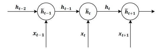
Figure 1.
Structural diagram of the GRU network.
For detailed descriptions of the GRU’s internal gating mechanisms (update gate, reset gate, candidate hidden state, and hidden state update), we refer readers to the foundational work by Cho et al. [18].
2.2. Grid Search Method
The grid search method is one of the most commonly used methods for exploring the hyperparameter configuration space [19]. This method can be regarded as an exhaustive search or brute-force search strategy, where it evaluates all possible combinations of hyperparameters within the given configuration grid to find the optimal solution [20]. The core mechanism lies in performing a Cartesian product operation on the pre-defined finite set of parameter values defined by the user, evaluating the performance of each combination.
When there are k hyperparameters and each parameter has n candidate values, the computational complexity of the grid search will increase exponentially at a rate of [21]. This characteristic makes it more suitable for optimization scenarios in low-dimensional configuration spaces. In the current research scenario, the hyperparameters to be optimized for the GRU model mainly include the following four categories: time step, hidden layer unit number, learning rate, and training epoch. Their low-dimensional nature and discrete value characteristics keep the computational complexity of the grid search within a controllable range, enabling efficient identification of the optimal parameter combination.
3. Data
Based on the architecture proposed in Section 2, this subsection introduces the data used for conducting experiments on the above architecture and the reasons for selecting these data. The research data consist of the following three parts: the TEC of the ionosphere, closely related solar 10.7 cm radio flux (F10.7), and number of sunspots (R).
3.1. TEC
The TEC used in this study was sourced from the Eglin Observatory in Florida, USA. The TEC data were generated by the Digisonde-Portable-Sounder-4D using the autoscaling algorithm. The equipment was manufactured by Lowell Digisonde International in Lowell, MA, USA. And the TEC was obtained from the Global Ionospheric Radio Observation Database, and the URL is as follows: https://giro.uml.edu/didbase/ (accessed on 10 October 2023) [22]. Figure 2 shows that this station is located at a 30°29′ north latitude and a 86°30’ west longitude. The reason for choosing the Eglin station as the location for model validation is that this station has an 18-year-long, continuous, and publicly available TEC data record from 2004 to 2022. The relatively complete data are beneficial for the GRU model to capture the long-term trend in the TEC data. Furthermore, in the mid-latitudes, the TEC of the ionosphere is usually at a moderate level, with its value significantly higher than that in high-latitude regions but lower than the notable equatorial anomaly peak. Compared to more dynamic equatorial or polar regions, the thickness variation in the ionosphere in the mid-latitudes is relatively more stable [23]. Therefore, it serves as an ideal initial testing platform for evaluating the core predictive capability of the proposed grid-search optimization GRU method under typical conditions. It is particularly important to note that the achieved Root Mean Square Error (RMSE) performance is applicable only to this mid-latitude region. Similar error levels may not directly apply to the equatorial region and high-latitude/polar regions. The upper-right corner shows the data distribution map of Eglin station, with data missing in 2004 and 2009.
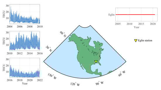
Figure 2.
Location of Eglin station.
This study focuses on analyzing the long-term trend of TEC. Therefore, the original TEC data were processed into monthly median data: the daily 24 h observation data were calculated as the monthly median hourly, generating a monthly average TEC sequence with hourly time resolution. This processing strategy effectively suppresses short-term disturbance noise through median filtering, while retaining the long-term correlation features such as solar activity cycles and seasonal variations [24]. The monthly median value of the mathematical expression of the TEC is as follows:
where h represents the hour, and m represents the month. D represents the actual number of observation days in the current month, and TECd(h,m) is the observation value at the h-th hour of the d-th day. By analyzing the data from 2004 to 2021, it was found that there were data gaps in some periods. The median TEC data for the month are shown on the left side of Figure 3, and TECU is the unit of TEC, where 1TECU = 1 × 10¹⁶ electrons/m2.
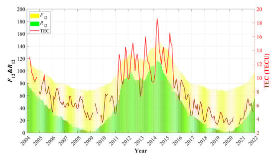
Figure 3.
R12, F12, and TEC data.
3.2. F10.7
F10.7 is the core input parameter of the ionosphere parameter prediction model, with the unit being the solar flux unit (sfu,1 sfu = 10−22 W·m−2·Hz−1) [25]. Its physical meaning is the solar radio radiation intensity at the 10.7 cm wavelength (2.8 GHz). The F10.7 data are provided by the Space Weather Prediction Center of the National Oceanic and Atmospheric Administration, and the URL is as follows: https://www.ngdc.noaa.gov/stp/space-weather/solar-data/ (accessed on 10 October 2023). F10.7 quantifies the ionization efficiency of neutral gas in the ionosphere due to solar electromagnetic radiation, directly influencing TEC’s spatial distribution and temporal evolution. Studies have shown that F10.7 is significantly positively correlated with the peak electron density of the ionosphere and TEC [26]. To characterize temporal variations in ionospheric parameters and develop predictive models, the twelve-monthly smoothed value of F10.7 is a key indicator for quantifying solar activity dynamics in ionospheric prediction studies [27].
3.3. Sunspot
The sunspot relative number (R) is a classic parameter used to characterize the intensity of magnetic field activity on the surface of the Sun. It was proposed and continuously released by the Royal Observatory of Belgium in 1849 [28]. R data are provided by the Belgian Solar Influences Data Analysis Center. The standardized sequence released by this institution, and the URL is as follows: https://www.sidc.be/silso/datafiles (accessed on 10 October 2023) is calculated using Equation (3) [29], as follows:
where g represents the number of visible solar surface sunspots, s represents the total number of individual sunspots, and k is the correction coefficient of the observation station. The long-term variation in the R value directly reflects the periodic oscillation of the solar magnetic field activity. Further, it regulates the total solar radiation and the intensity of EUV/XUV radiation [30]. Since EUV radiation is the primary energy source for ionizing the ionosphere, a significant nonlinear correlation exists between R and TEC [2]. Analogous to the application of F10.7, the 12-month smoothed R value functions as a complementary solar activity metric in ionospheric modeling research, particularly for capturing long-term cyclical variations essential for predictive accuracy [31].
The calculation formula for the twelve-monthly smoothed value of the sun activity parameter is as follows:
where MS denotes the solar activity parameter requiring 12-month smoothing, and indicates its monthly mean value. The variable n specifies the target month for calculating the moving average, with i being its sequential index. Post-smoothing, the transformed R and F10.7 indices are labeled R12 and F12, respectively.
TEC exhibits periodic daily and annual cycles. Its level and variation range are highly correlated with the level of solar activity [32]. Figure 3 demonstrates the temporal evolution of R12, F12, and monthly averaged TEC (derived from hourly median values) during 2004–2022. While R12 and F12 exhibit analogous macro-trends, nuanced differences emerge in their temporal profiles. Notably, both solar indices maintain positive correlations with TEC variations.
Our parameter selection gives priority to F10.7 and R, because they are widely used solar indices in ionospheric research, and they are directly related to solar ultraviolet radiation and magnetic activity cycles. For instance, papers by Maruyama et al. [33] and Yang et al. [34] both use F10.7 and R to predict TEC.
4. Modeling
This section describes the modeling process as shown in Figure 4. First, data preprocessing was performed (Figure 4a), including using statistical learning methods to impute missing TEC observation data. Then, a GRU model was constructed (Figure 4b), with hyperparameters determined by the grid-search optimization method, using the RMSE of the validation set as the evaluation criterion. Finally, the optimal parameter combination was used to complete the model building.
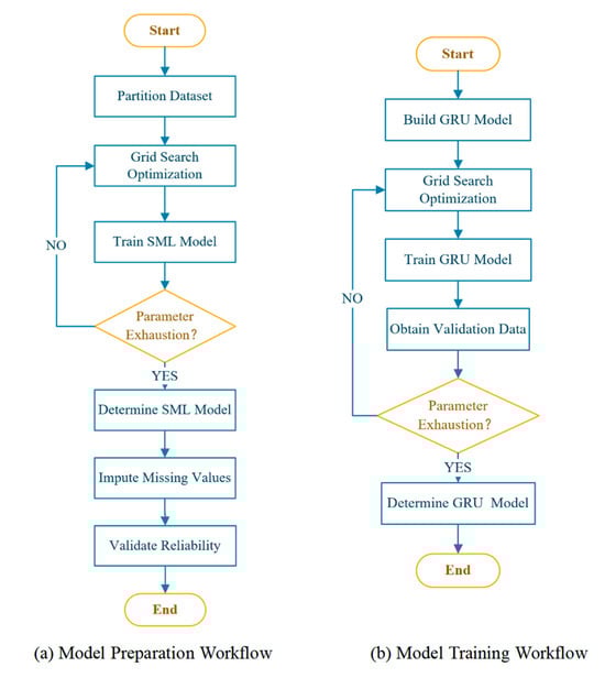
Figure 4.
Schematic diagram of the TEC prediction model established based on a GRU.
4.1. Modeling Preparation
This study divides and constructs the training, validation, and test sets based on the 11-year periodic characteristics of solar activity. The training set selects data from 2004 to 2014, totaling 132 months; the validation set covers data from 2015 to 2018, totaling 48 months; and the test set uses data from 2019 to 2020, totaling 24 months.
Deep learning models such as GRU have strict requirements for the integrity of the input sequence. Missing data may cause deviations in the update of network weights and affect the continuous learning of temporal features [35]. The rate of missing TEC data in the observation is relatively low. The missing rate of the entire dataset at each time point is lower than 3.03%, as shown in Figure 5. Therefore, the statistical machine learning method proposed by Liu et al. [10] is considered to fill in the missing values.
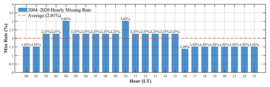
Figure 5.
Proportion of absence (unit: %).
According to Reference [10], the solar activity index (R, F10.7) has a multi-dimensional nonlinear mapping relationship with TEC. Based on the SML theory, using trigonometric basis functions can characterize TEC’s temporal correlation, such as annual and semi-annual cycles. Moreover, a polynomial is introduced to describe the nonlinear effect of the solar activity index [10]. Specifically, as follows:
where I12 denotes the solar activity parameter, m corresponds to the month index (integer values), K and J define the maximum expansion orders for harmonic and polynomial components, respectively, with and as the associated coefficients. Model calibration is achieved through least squares optimization to determine these parameters. I12, K, and J are selected based on the RMSE as the evaluation index, as shown in the following formula:
where represents the model predicted value, TECi represents the actual observed value, and N represents the total data quantity.
To ensure the accuracy of data filling, we trained the model using the data from the TEC training dataset collected in this paper and determined the final SML-based model using the RMSE of the validation dataset with the measured TEC. Figure 6 shows the RMSE values of the model under different parameter combinations.
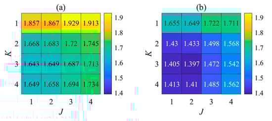
Figure 6.
Heatmap of RMSE values predicted by the SML-based model under different input parameter combinations: (a) solar activity index is R12; (b) solar activity index is F12.
The experimental results in Figure 7 indicate optimal parameter combinations. For an R12 index with K = 3 and J = 1, the SML model achieves a minimum RMSE of 1.64 TECU. Similarly, using the F12 index with K = 3 and J = 2 yields an improved performance with the RMSE reduced to 1.40 TECU. Therefore, in the final model, F12 is used, K is selected as 3, and J is chosen as 2, as shown in the following equation:
where m represents the corresponding month.
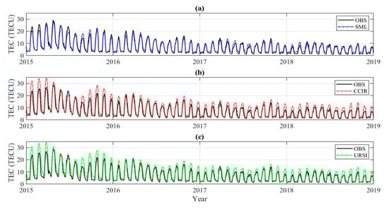
Figure 7.
Comparison chart of the predicted values of the SML-based, CCIR, and URIS models on the validation set with those of OBS: (a) SML-based; (b) CCIR; (c) URSI.
The CCIR and URSI models are widely used sub-models within the IRI model, serving as standard benchmarks for ionospheric parameter predictions. The CCIR model utilizes spherical harmonic functions combined with universal time harmonic functions to describe the global distribution of parameters such as foF2 and M(3000)F2. Primarily based on historical data (with observation stations predominantly located in the Northern Hemisphere), it relies on statistical methods to establish a global-scale parametric representation and holds distinct value for studying long-term variation trends. However, this dependency limits its accuracy in capturing fine structures, particularly in equatorial anomaly zones. In contrast, the URSI model integrates more modern and globally balanced datasets, significantly improving coverage in the Southern Hemisphere and equatorial regions. Although both models demonstrate comparable global accuracy, URSI outperforms CCIR in low-latitude regions [9]. The URSI utilizes data from modern global observation networks and employs complex algorithms to resolve physical mechanisms within the ionosphere, providing greater accuracy for short-term predictions, particularly at mid- and low latitudes.
We chose these models as references because they represent current international standards and have been applied in many comparative studies. For instance, studies by Yu et al. [17], Sezen et al. [36], and Liu et al. [37] all used these models for comparison. The model data were obtained from NASA’s Instant Run platform, and the URL is as follows: https://kauai.ccmc.gsfc.nasa.gov/instantrun/iri/ (accessed on 21 April 2025), where inputting specific coordinates, time parameters, and data types yields corresponding outputs. As delineated by Zhen et al. (2024) [38], these two model types play complementary roles in ionospheric research. Their synergistic application, therefore, enables comprehensive coverage of scientific needs—from physical mechanism analysis to long-term evolution studies—ultimately enriching the understanding of the ionosphere.
The comparison results are shown in Figure 7. The RMSEs of the predicted values of the CCIR and URSI relative to the measured values were 3.01 TECU and 3.06 TECU, respectively, which are greater than 1.40 TECU. This proves the accuracy of the SML-based method in filling in missing data.
Figure 8 presents a periodic characteristic comparison analysis of the data sequences before and after interpolation. The results show that the dataset filled by the SML-based model is highly consistent with the original observations regarding diurnal variation patterns and seasonal fluctuation characteristics. This also proves the reliability of filling data with the SML method.
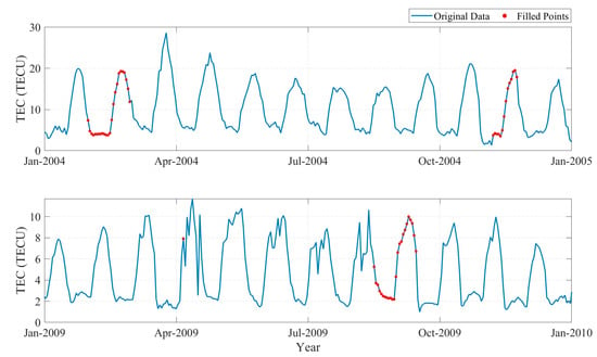
Figure 8.
Comparison before and after interpolation.
In the end, this study employed min–max normalization to map TEC, R12, and F12 to the interval [0, 1] to accelerate the gradient convergence of the GRU network and eliminate the influence of feature scale differences [31].
4.2. Model Training
While building the GRU prediction model, we first established the basic framework of the neural network. The model consists of an input layer, a GRU layer, and a fully connected output layer. The GRU layer serves as the core processing unit and captures the temporal dependency features in the TEC sequence. This network uses the sigmoid and tanh functions as activation functions, takes the mean square error as the loss function, and uses the Adam optimizer for optimization [1]. The model input is a time series of the timestep length, predicting the value of the next timestamp. The time step unit is in months. Although the dataset contains data for each hour (as mentioned above, TEC represents the monthly median, and the solar activity index is the twelve-monthly smoothed value), when inputting the data into the model, we organized it into monthly time series samples by hour for input.
Subsequently, we constructed four sets of data input schemes for a horizontal comparison:
- Only the original TEC observation values (OBS);
- OBS combined with the R12 index;
- OBS combined with the F12 index;
- OBS combined with both the R12 and F12 dual indices.
We set the fixed batch size to 64. Then, we conducted the grid-search optimization method separately under four feature input schemes, and the obtained hyperparameters are as follows:
- Number of training epochs: the search range is from 20 to 26;
- Learning rate: the search range is from 0.001 to 0.005, with a step size of 0.001;
- Number of hidden layer units: the search range is 120 to 136, with a step size of 4;
- Time step: The search range is 12 and 24;
- Number of GRU layers: the search range is 1 and 2.
To quantitatively evaluate the training effect of the GRU neural network model, we used the RMSE to assess the prediction results. We selected the input data and parameter group corresponding to the minimum RMSE value in the validation set as the final model. Taking the model with input as OBS, R12, and F12, and a single-layer GRU structure and a 12 h time step as an example, Figure 9 shows the RMSE between the predicted values and the observed values within the parameter search range.
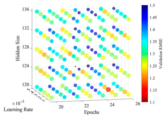
Figure 9.
RMSE between the model validation values and the measured values within the search range.
The other three input combinations were also optimized using the grid search method, and the results are shown in Table 1. Among them, the prediction performance of the combination of inputs OBS, R12, and F12 was the best (minimum RMSE = 1.15 TECU). Based on this, OBS, R12, and F12 were finally selected as the input, and the optimal parameter combination is as follows:

Table 1.
Optimization results and performance comparison of hyperparameters for different input combinations.
- Number of training epochs = 25;
- Learning rate = 0.003;
- Number of hidden units = 120;
- Time step = 12;
- Number of GRU layers = 1.
5. Discussion
To conduct a comprehensive evaluation of the model’s performance established in this paper, the model was tested using the test dataset, and the obtained results were compared and analyzed with those of the IRI (including CCIR and URSI models) and SML-based models. It should be noted that, unlike the comparison models, such as SML and GRU, which can ingest hourly-updated measurements, the IRI, as an empirical model, lacks the capability of real-time data access. This disparity in data temporality may introduce a systematic asymmetry in performance benchmarking. Nevertheless, the GRU’s capability to integrate real-time data holds significant operational value for space weather forecasting.
Figure 10 presents the observed values of the TEC, while Figure 11 shows the prediction errors (predicted–observed) of the CCIR, URSI, SML-based, and GRU models. All times are expressed in LT without daylight-saving adjustments. The following can be seen from the figure:
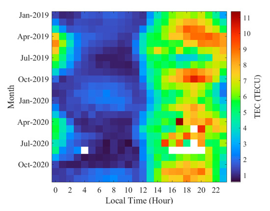
Figure 10.
The observed values of the TEC.
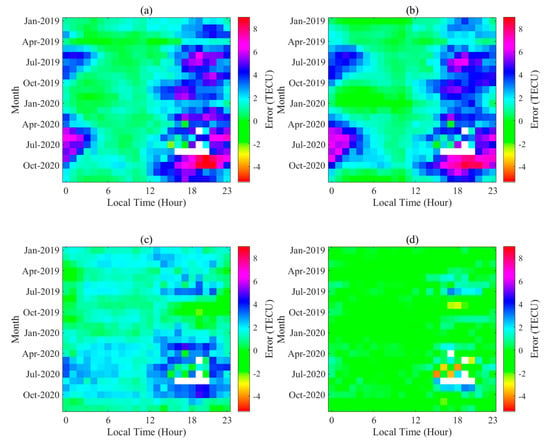
Figure 11.
Error of the comparison model: (a) CCIR; (b) URSI; (c) SML; (d) GRU.
- (1)
- All models demonstrate capability in tracking long-term TEC trends yet exhibit varying degrees of predictive accuracy across temporal segments.
- (2)
- Comparative analysis reveals distinct error patterns, as follows: The CCIR and URSI models systematically overestimate TEC measurements, particularly from LT = 20 to LT = 1 the next day. The SML approach shows elevated predictions between 22:00 and 10:00 LT. The proposed GRU model maintains prediction stability across all time segments without notable systematic bias.
- (3)
- In the predictions of different hours, the GRU model demonstrated the highest prediction accuracy, with a significant advantage.
To comprehensively evaluate the predictive performance of the model, in addition to using the RMSE as the evaluation metric, the Mean Absolute Error (MAE) and Relative Root Mean Squared Error (RRMSE) are further introduced as supplementary indicators. The specific calculation formulas are as follows:
where represents the model’s predicted value, represents the observed value, N represents the total amount of the data being analyzed, and represents the arithmetic mean of the observed values, that is, the following:
Figure 12 presents the hourly RMSEs, MAEs, and RRMSEs of the predicted values and observations for the four models. The results show the following:
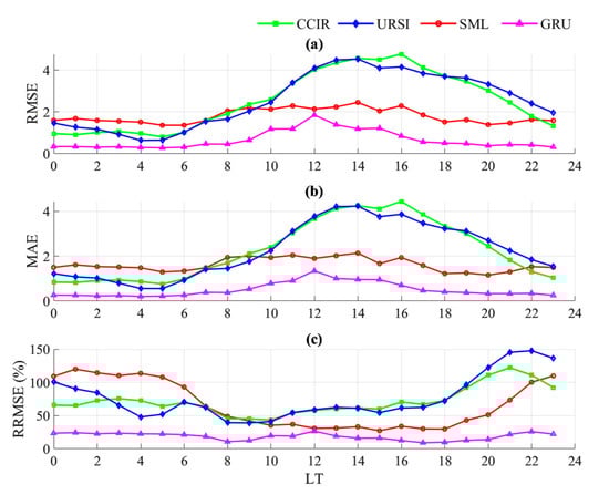
Figure 12.
RMSE, MAE, and RRMSE between the predicted values of the four models and OBS obtained by hourly statistics: (a) RMSE; (b) MAE; (c) RRMSE.
- (1)
- Throughout the entire testing period from 2019 to 2020, the relative magnitudes of the error indicators of the four models remained consistent. In other words, at the same point in time, regardless of the error indicator, the order of the error magni-tudes of the four models is consistent.
- (2)
- For the 24 h prediction, there are significant differences in error among the various models. From the perspectives of the RMSE and MAE, the errors of the CCIR and URSI models are relatively large, from LT = 11 to LT = 18. Analyzing the RRMSE, the SML-based model exhibited larger errors from LT = 23 to LT = 5 the next day, the CCIR from LT = 19 to LT = 23, and the URSI from LT = 19 to LT = 0 the next day.
- (3)
- Considering the overall performance of the 24 h prediction throughout the day, the GRU model’s RMSE, MAE, and RRMSE are significantly lower than those of the other models, indicating that the GRU model has higher prediction accuracy and better performance.
- (4)
- Further comparing the errors between the predicted values and the observed values of the GRU model showed the following: from LT = 17 to LT = 9 the next day, the RMSE and MAE are small, while from LT = 10 to LT = 16, the RMSE and MAE are large. This indicates that the absolute error of the GRU model predictions is significantly higher during LT = 10–16. However, the RRMSE performance is relatively consistent per hour because it reflects the relative differences, and the overall performance of the GRU model is relatively balanced.
Figure 13 shows the four models’ RMSEs, MAEs, and RRMSEs compared with observations for different seasons (spring: March–May; summer: June–August; autumn: September–November; winter: December–February). The results indicate the following:
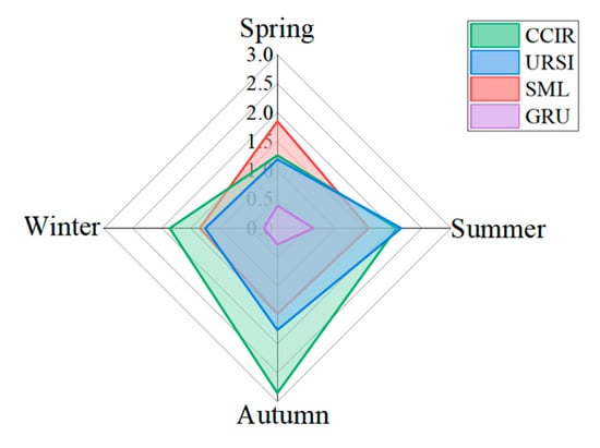
Figure 13.
RMSE between the predicted values of the four models and OBS, calculated on a seasonal basis.
- (1)
- The SML-based model exhibits greater prediction errors in spring than other models due to inadequate representation of noontime ionospheric disturbances triggered by enhanced solar radiation [39].
- (2)
- CCIR shows large errors in autumn/winter because it ignores frequent magnetic storms in winter [40].
- (3)
- The GRU model achieves the smallest prediction errors across all seasonal metrics. However, its error is relatively higher in summer. This is because of physical processes not captured by the model (such as rapid electron loss at night via recombination), which represent a common challenge for purely data-driven methods like GRU to learn [41].
Figure 14 presents the statistics of MAE and RMSE between the predicted values and OBS for each model. From this figure, we can see the following:
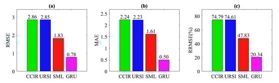
Figure 14.
RMSE, MAE, and RRMSE of the predicted values of the four models and the OBS: (a) RMSE; (b) MAE; (c) RRMSE.
- (1)
- Regarding the RMSE, the GRU model has the smallest RMSE of 0.78 TECU. Compared with the SML-based model, CCIR model, and URSI model, it was reduced by 1.05 TECU, 2.08 TECU, and 2.07 TECU, respectively;
- (2)
- Regarding the MAE, the GRU model has the smallest MAE of 0.50 TECU. Compared with the SML-based model, CCIR model, and URSI model, it was reduced by 1.11 TECU, 1.74 TECU, and 1.73 TECU, respectively;
- (3)
- Regarding the RRMSE, the GRU model has the smallest RRMSE of 20.34%. Compared with the SML-based model, CCIR model, and URSI model, it was reduced by 27.49%, 54.45%, and 54.27%, respectively;
- (4)
- Overall, the GRU model significantly outperforms the RMSE, MAE, and RRMSE comparison models. The error reduction ranges from 1.05 to 2.08 TECU and 27.49% to 54.45%, demonstrating comprehensive performance advantages.
6. Conclusions
This paper proposes a prediction model of ionospheric TEC based on a grid-optimization GRU. This model was tested and evaluated using data from Eglin station as a case study. A detailed comparison and analysis were conducted against existing models, including SML-based, CCIR, and URSI models. The results show that the GRU model has significant advantages in the prediction of TEC. Specifically, the RMSE of the GRU model was 72.73%, 72.64%, and 57.38% lower than those of the CCIR, URSI, and SML models, respectively. Additionally, the MAE was reduced by 77.73% and 77.58% compared to the CCIR and URSI models, respectively, and by 68.94% compared to the SML-based model. These results indicate that the GRU model can effectively capture the long-term trend of TEC and shows good predicting effects at different seasonal and hourly scales. Similarly, these results can demonstrate that the GRU model has broad applicability and practical value and can be extended to the prediction of other ionospheric parameters (such as foF2 and hmF2). In the future, we plan to further research and verify the GRU model using multi-station data to evaluate its TEC prediction performance across different stations.
Author Contributions
Conceptualization, S.Z., Z.Y., Q.Y., and J.W.; methodology, S.Z., Z.Y., and Q.Y.; software, S.Z. and Z.Y.; validation, S.Z. and Z.Y.; formal analysis, S.Z. and Z.Y.; investigation, S.Z., Z.Y., and Q.Y.; resources, Q.Y. and J.W.; data curation, S.Z., Z.Y., and Q.Y.; writing—original draft preparation, S.Z. and Z.Y.; writing—review and editing, Q.Y. and J.W.; visualization, S.Z. and Z.Y.; supervision, Q.Y. and J.W.; project administration, Q.Y. and J.W.; funding acquisition, J.W. All authors have read and agreed to the published version of the manuscript.
Funding
This research received no external funding.
Institutional Review Board Statement
Not applicable.
Informed Consent Statement
Not applicable.
Data Availability Statement
The original contributions presented in the study are included in the article, further inquiries can be directed to the corresponding author.
Acknowledgments
The ionospheric TEC data used in this study were obtained from the Global Ionospheric Radio Observatory (GIRO) database, and the URL is as follows: https://giro.uml.edu/didbase/ (accessed on 10 October 2023). We gratefully acknowledge the DIDBase team and Bodo W. Reinisch at the University of Massachusetts Lowell for providing access to the Eglin station (Station ID: E31) observational data. This research strictly follows GIRO’s “Rules of the Road”.
Conflicts of Interest
The authors declare no conflict of interest.
Abbreviations
The following abbreviations are used in this manuscript:
| ANNs | Artificial Neural Networks |
| CCIR | International Radio Consultative Committee |
| F10.7 | Solar 10.7 cm Radio Flux |
| foF2 | Ionospheric F2 layer |
| GRU | Gate Recurrent Unit |
| IRI | International Reference Ionosphere |
| LSTM | Long Short-Term Memory Network |
| MAE | Mean Absolute Error |
| OBS | Observations |
| R | Sunspot Relative Number |
| RNN | Recurrent Neural Network |
| RRMSE | Relative Root Mean Squared Error |
| SIDC | Solar Influences Data Analysis Center |
| SML | Statistical Machine Learning |
| sfu | Solar Flux Unit |
| TEC | Total Electron Content |
| URSI | International Union of Radio Science |
| LT | Local Time |
References
- Ming, F.X.; Ma, J.S. Study on Ionospheric Anomaly During Geomagnetic Storm by Beidou GEO Satellites. Geospat. Inf. 2023, 21, 100–103. [Google Scholar]
- Liu, L.B.; Wan, W.X.; Chen, Y.D.; Le, H.J. Solar activity effects of the ionosphere: A brief review. Chin. Sci. Bull. 2011, 56, 1202–1211. [Google Scholar] [CrossRef]
- Zhang, H.P. Research on China’s Regional Ionosphere Monitoring and Delay Correction Based on Ground-Based GPS. Ph.D. Thesis, Graduate University of Chinese Academy of Sciences, Shanghai Astronomical Observatory, Shanghai, China, 2006. [Google Scholar]
- Priyadarshi, S. A Review of Ionospheric Scintillation Models. Surv. Geophys. 2015, 36, 295–324. [Google Scholar] [CrossRef]
- Yuan, Y.B. Study on Theories and Methods of Correcting Ionospheric Delay and Monitoring Ionosphere Based on GPS. Ph.D. Thesis, Graduate University of Chinese Academy of Sciences, Institute of Geodesy and Geophysics, Wuhan, China, 2002. [Google Scholar]
- Yao, Y.B.; Chen, X.X.; Kong, J.; Zhou, C.; Liu, L.; Shan, L.L.; Guo, Z.H. An Updated Experimental Model of IG Indices Over the Antarctic Region via the Assimilation of IRI2016 With GNSS TEC. IEEE Trans. Geosci. Remote Sens. 2021, 59, 1700–1717. [Google Scholar] [CrossRef]
- Zhang, W.; Huo, X.L.; Yuan, Y.B.; Li, Z.S.; Wang, N.B. Algorithm Research Using GNSS-TEC Data to Calibrate TEC Calculated by the IRI-2016 Model over China. Remote Sens. 2021, 13, 4002. [Google Scholar] [CrossRef]
- Bilitza, D. International Reference Ionosphere 2000. Radio Sci. 2001, 36, 261–275. [Google Scholar] [CrossRef]
- Bilitza, D.; Altadill, D.; Truhlik, V.; Shubin, V.; Galkin, I.; Reinisch, B.; Huang, X. International Reference Ionosphere 2016: From ionospheric climate to real-time weather predictions. Space Weather-Int. J. Res. Appl. 2017, 15, 418–429. [Google Scholar] [CrossRef]
- Liu, Y.R.; Wang, J.; Yang, C.; Zheng, Y.; Fu, H.P. A Machine Learning-Based Method for Modeling TEC Regional Temporal-Spatial Map. Remote Sens. 2022, 14, 5579. [Google Scholar] [CrossRef]
- Jia, W.K.; Zhao, D.A.; Ding, L. An optimized RBF neural network algorithm based on partial least squares and genetic algorithm for classification of small sample. Appl. Soft Comput. 2016, 48, 373–384. [Google Scholar] [CrossRef]
- Hu, X.; Zhou, C.; Zhao, J.; Liu, Y.; Liu, M.; Zhao, Z. The ionospheric foF2 prediction based on neural network optimization algorithm. Chin. J. Radio Sci. 2018, 33, 708–716. [Google Scholar] [CrossRef]
- Zhang, F.; Zhou, C.; Wang, C.; Zhao, J.; Liu, Y.; Xia, G.; Zhao, Z. Global ionospheric TEC prediction based on deep learning. Chin. J. Radio Sci. 2021, 36, 553–561. [Google Scholar]
- Li, W.; Zhao, D.S.; He, C.Y.; Hu, A.D.; Zhang, K.F. Advanced Machine Learning Optimized by The Genetic Algorithm in Ionospheric Models Using Long-Term Multi-Instrument Observations. Remote Sens. 2020, 12, 866. [Google Scholar] [CrossRef]
- Weng, J.X.; Liu, Y.R.; Wang, J. A Model-Assisted Combined Machine Learning Method for Ionospheric TEC Prediction. Remote Sens. 2023, 15, 2953. [Google Scholar] [CrossRef]
- Xia, G.Z.; Liu, Y.; Wei, T.F.; Wang, Z.K.; Huang, W.Q.; Du, Z.T.; Zhang, Z.B.A.; Wang, X.; Zhou, C. Ionospheric TEC forecast model based on support vector machine with GPU acceleration in the China region. Adv. Space Res. 2021, 68, 1377–1389. [Google Scholar] [CrossRef]
- Yu, Q.; Men, X.; Wang, J. A Prediction Model of Ionospheric Total Electron Content Based on Grid-Optimized Support Vector Regression. Remote Sens. 2024, 16, 2701. [Google Scholar] [CrossRef]
- Cho, K.; Van Merriënboer, B.; Gulcehre, C.; Bahdanau, D.; Bougares, F.; Schwenk, H.; Bengio, Y. Learning phrase representations using RNN encoder-decoder for statistical machine translation. arXiv 2014. [Google Scholar] [CrossRef]
- Injadat, M.; Moubayed, A.; Nassif, A.B.; Shami, A. Systematic ensemble model selection approach for educational data mining. Knowl.-Based Syst. 2020, 200, 105992. [Google Scholar] [CrossRef]
- Injadat, M.; Moubayed, A.; Nassif, A.B.; Shami, A. Multi-split optimized bagging ensemble model selection for multi-class educational data mining. Appl. Intell. 2020, 50, 4506–4528. [Google Scholar] [CrossRef]
- Lorenzo, P.R.; Nalepa, J.; Ramos, L.S.; Pastor, J.R. Hyper-Parameter Selection in Deep Neural Networks Using Parallel Particle Swarm Optimization. In Proceedings of the Genetic and Evolutionary Computation Conference (GECCO), Berlin, Germany, 15–19 July 2017; pp. 1864–1871. [Google Scholar]
- Reinisch, B.W.; Galkin, I.A. Global Ionospheric Radio Observatory (GIRO). Earth Planets Space 2011, 63, 377–381. [Google Scholar] [CrossRef]
- Homam, M.J. Latitudinal Effect on Total Electron Content Variations. In Proceedings of the International Symposium on Antennas and Propagation (ISAP), Kaohsiung, Taiwan, 2–4 December 2014; pp. 127–128. [Google Scholar]
- Zhao, G.C.; Zhang, L.; Wu, F.B. Application of improved median filtering algorithm to image de-noising. J. Appl. Opt. 2011, 32, 678–682. [Google Scholar]
- Tapping, K.F. The 10.7 cm solar radio flux(F10.7). Space Weather-Int. J. Res. Appl. 2013, 11, 394–406. [Google Scholar] [CrossRef]
- Hathaway, D.H. The Solar Cycle. Living Rev. Sol. Phys. 2015, 12, 4. [Google Scholar] [CrossRef] [PubMed]
- Liu, C.X.; Zhang, M.L.; Wan, W.X.; Liu, L.; Ning, B.Q. Modeling M(3000)F2 based on empirical orthogonal function analysis method. Radio Sci. 2008, 43, 1–8. [Google Scholar] [CrossRef]
- Clette, F.; Berghmans, D.; Vanlommel, P.; Van der Linden, R.A.M.; Koeckelenbergh, A.; Wauters, L. From the Wolf number to the International Sunspot Index: 25 years of SIDC. Adv. Space Res. 2007, 40, 919–928. [Google Scholar] [CrossRef]
- Sabour, S.; Frosst, N.; Hinton, G.E. Dynamic Routing Between Capsules. In Proceedings of the 31st Annual Conference on Neural Information Processing Systems (NIPS), Long Beach, CA, USA, 4–9 December 2017. [Google Scholar]
- Bhowmik, P.; Nandy, D. Prediction of the strength and timing of sunspot cycle 25 reveal decadal-scale space environmental conditions. Nat. Commun. 2018, 9, 5209. [Google Scholar] [CrossRef]
- Weerakody, P.B.; Wong, K.W.; Wang, G.J.; Ela, W. A review of irregular time series data handling with gated recurrent neural networks. Neurocomputing 2021, 441, 161–178. [Google Scholar] [CrossRef]
- Shreedevi, P.R.; Choudhary, R.K.; Yadav, S.; Thampi, S.V.; Ajesh, A. Variation of the TEC at a dip equatorial station, Trivandrum and a mid latitude station, Hanle during the descending phase of the solar cycle 24 (2014-2016). J. Atmos. Sol.-Terr. Phys. 2018, 179, 425–434. [Google Scholar] [CrossRef]
- Maruyama, T. Regional reference total electron content model over Japan based on neural network mapping techniques. Ann. Geophys. 2007, 25, 2609–2614. [Google Scholar] [CrossRef]
- Yang, N.; Le, H.J.; Liu, L.B. Statistical analysis of ionospheric mid-latitude trough over the Northern Hemisphere derived from GPS total electron content data. Earth Planets Space 2015, 67, 196. [Google Scholar] [CrossRef]
- Xu, T.; Wu, Z.S.; Wu, J.; Wu, J. Solar cycle variation of the monthly median foF2 at Chongqing station, China. Adv. Space Res. 2008, 42, 213–218. [Google Scholar] [CrossRef]
- Sezen, U.; Gulyaeva, T.L.; Arikan, F. Performance of Solar Proxy Options of IRI-Plas Model for Equinox Seasons. J. Geophys. Res. Space Phys. 2018, 123, 1441–1456. [Google Scholar] [CrossRef]
- Liu, L.; Zou, S.S.; Yao, Y.B.; Wang, Z.H. Forecasting Global Ionospheric TEC Using Deep Learning Approach. Space Weather-Int. J. Res. Appl. 2020, 18, e2020SW002501. [Google Scholar] [CrossRef]
- Zhen, W.M.; Ming, O.; Zhu, Q.L. Review on ionospheric sounding and modeling. Wuhan Univ. J. Nat. Sci. 2023, 38, 625–645. [Google Scholar] [CrossRef]
- Zhang, Y.; Yu, Y.; Duan, W. The spring prediction barrier of ENSO in retrospective prediction experiments as shown by the four coupled ocean-atmosphere models. Acta Meteorol. Meteorol. Sinica 2012, 70, 506–519. [Google Scholar]
- Wang, J.; Zhang, T.; Yang, W.; Zhang, X. Measurement and analysis of atmospheric radio noise. J. China Ins. Comm. 2000, 21, 86–90. [Google Scholar]
- Kong, X.; Zheng, W.; Zhang, X.; Wang, M.; Shan, F.; Zhao, Q. Energy-saving control method of air conditioning in mushroom house based on data - physics mixed model. Trans. Chin. Soc. Agric. Eng. 2025, 41, 309–317. [Google Scholar]


Disclaimer/Publisher’s Note: The statements, opinions and data contained in all publications are solely those of the individual author(s) and contributor(s) and not of MDPI and/or the editor(s). MDPI and/or the editor(s) disclaim responsibility for any injury to people or property resulting from any ideas, methods, instructions or products referred to in the content. |
© 2025 by the authors. Licensee MDPI, Basel, Switzerland. This article is an open access article distributed under the terms and conditions of the Creative Commons Attribution (CC BY) license (https://creativecommons.org/licenses/by/4.0/).