Model-Driven Clock Synchronization Algorithms for Random Loss of GNSS Time Signals in V2X Communications

Abstract

Onboard Vehicle-to-Everything (V2X) communication technology is being widely implemented in domains such as intelligent driving, vehicle–road cooperation, and smart transportation. Nevertheless, time synchronization in V2X systems suffers from instability due to the random loss of Global Navigation Satellite System (GNSS) Pulse-Per-Second (PPS) signals. To address this challenge, a model-driven local clock correction approach is proposed. Leveraging probability theory and mathematical statistics, models for the randomly lost GNSS PPS signals are developed. High-order polynomials are used to model local clocks. An optimized Kalman-filter-based time compensation algorithm is then devised to compensate for time errors during PPS signal loss. A software-based task-scheduling solution for precision-time synchronization is developed. An experimental testbed was then built to measure both terminal clocks and PPS signals. The proposed algorithm was integrated into the V2X terminals. Results show that the full-value PPS signals follow an exponential distribution. The onboard clock correction algorithm operates stably across three V2X terminals and accurately predicts clock variations. Furthermore, the virtual clocks achieve an average absolute error of 1.1 μs and a standard deviation of 16 μs, meeting the time synchronization requirements for V2X communication in intelligent connected vehicles.

1. Introduction

With the development of next-generation communication technology, Vehicle-to-Everything (V2X) wireless communication has rapidly advanced and is increasingly deployed for collaborative services, including vehicle platooning, collision warning, edge computing, and remote driving [1,2], which enhances driving efficiency and safety. Accurate clock synchronization in V2X vehicle intelligent terminals is critical, ensuring precise temporal sequencing and timely information transmission—essential prerequisites for the normal operation of all V2X services. However, the heterogeneity and high-speed mobility inherent in vehicular networks present significant clock synchronization challenges due to node heterogeneity, intermittent connectivity, and rapid topology changes [3,4].

Based on different clock reference sources, V2X terminal clock synchronization methods can be categorized into network-based and GNSS-based approaches. Network-based time synchronization methods rely on reference signal transmission through network nodes, utilizing protocols such as spanning tree and broadcast. Ansere et al. proposed a spanning-tree-based time synchronization algorithm that improves synchronization accuracy by estimating random transmission delays using the principle of maximum likelihood [5]. Li et al. proposed a timestamp-free synchronization algorithm based on spanning trees, which reduces communication overhead by presetting response times without the need for timestamp exchange [6]. Haider et al. proposed a k-Medoids clustering-based broadcast synchronization algorithm, which sequentially broadcasts reference information from cluster heads to intra-cluster members, effectively expanding synchronization coverage [7]. Medani et al. introduced an offset table-based stabilized broadcast algorithm, in which reference nodes calculate and broadcast clock offset information to all nodes, thereby avoiding the overhead associated with mutual information exchange between receiving nodes [8]. However, network transmission delays and communication overhead inevitably impact the precision and speed of network synchronization. The slow convergence of spanning tree algorithms and the poor adaptability of broadcast-based clustering strategies to dynamic vehicular networks pose significant challenges for network synchronization technologies, restricting their applications in the Internet of Vehicles.

GNSS-based synchronization delivers high-precision timing with global coverage, widely deployed in military, aerospace, power systems, and network communications, typically achieving nanosecond-level timing accuracy [9,10]. It is minimally affected by transmission delays, producing clear advantages over network-based time synchronization. When GNSS signals are properly received, onboard receivers provide V2X terminals with time synchronization signals of Time of Day (TOD) and PPS. However, in non-line-of-sight scenarios such as obstructed environments, tunnels, and underground parking lots, GNSS signals may be degraded or lost, compromising terminal synchronization accuracy [11,12].

One method involves switching to backup clock sources, such as the GNSS Disciplined Oscillators (GNSSDO), mainly composed of phase detectors and voltage-controlled oscillators, which compensate for GNSS signal loss using historical measurement data [13,14]. Toan designed an FPGA-based adaptive drift correction algorithm for GPS-disciplined oscillators, which demonstrated a drift of less than 356 ns in the 1 PPS signal over a 24 h GNSS signal outage in outdoor environments [15]. Boehmer devised a temperature-compensated crystal oscillator [16]. This oscillator is designed to intermittently rectify the frequency drift occurring in GPS-disciplined oscillators. As a result, it maintains sub-5 μs synchronization. Although the GNSSDO possesses the capability to compensate for signal loss, it necessitates hardware support entailing substantial costs. This approach consistently maintains clock offset variance below 5 μs. Although GNSSDO can compensate for signal loss, they require costly hardware. Moreover, their operational stability remains vulnerable to multiple factors, including environmental temperature fluctuations, vibration shocks, and crystal aging, primarily due to their reliance on oscillator circuits.

Another approach leverages multi-GNSS technology to receive signals from multiple satellite constellations. Hasan et al. proposed a method utilizing commercial-grade multi-GNSS receivers, achieving near-full time availability in challenging environments such as those with trees, short overpasses, and bridges, with single-vehicle synchronization accuracy reaching ±2 μs [17,18]. However, under a complete GNSS signal blockage, synchronization deviation increases significantly, reaching up to 20 μs. Although the multi-GNSS technology enhances the availability of time synchronization signals, multi-GNSS receivers remain relatively expensive and are unable to prevent signal loss entirely. As revealed by our comprehensive assessment, V2X terminal devices utilize backup clock sources to ensure hardware-based synchronization when the GNSS PPS signal is lost. The implementation of this technology leads to an increase in cost and size. At present, the topic of onboard software-based synchronization via embedded software remains largely underexplored. The soft synchronization approach not only ensures accurate time synchronization but also compensates for the limitations of hard synchronization.

This paper proposes a novel model-driven time synchronization method for V2X terminals experiencing unstable GNSS signal reception. Our approach introduces two key innovations: (1) advanced GNSS PPS probability models and (2) a clock self-compensation algorithm. Crucially, the solution requires no additional hardware, significantly improving synchronization accuracy at minimal cost while maintaining compatibility with existing GNSS receivers. The subsequent content arrangement of this paper is outlined as follows: First, clock modeling and GNSS PPS signal characterization for V2X systems are described. Second, a virtual clock state-space model and Kalman Filter (KF)-based self-compensating synchronization algorithm are developed. Finally, experimental validation of proposed models and algorithms is conducted.

2. Models and Algorithms

2.1. Clock Model

2.1.1. Local Clock Model

Local clocks of V2X terminals derive from quartz crystal oscillators, subject to manufacturing processes, temperature, humidity, environmental noise, aging, and other factors. The oscillator frequency exhibits nonlinear variations over time, with local time obtained through temporal integration of this frequency.

$$C(t)={\displaystyle \frac{1}{f_0}}{\displaystyle {\int }_{t_0}^{t}f(t)dt}+C(t_0),$$

(1)

where t denotes the absolute time; f₀ denotes the nominal frequency of the crystal oscillator; f(t) denotes the actual frequency of the local clock at time t; C(t₀) represents the initial offset between the local time C(t) and the reference time t; and t₀ denotes the start time.

The nonlinear behavior of a local clock can be modeled as a polynomial function with superimposed Gaussian noise.

$$C(t)=a_n{t}^n+a_{\mathrm{n}-1}{t}^{n-1}+\dots +a_0+w(t),$$

(2)

where n denotes the highest order of the model; a_i represents the coefficient of the i-th order term in reference time t, where each coefficient corresponds to distinct clock characteristics, such as a₀ denotes phase deviation, a₁ denotes frequency offset and a₂ denotes frequency drift rate; and w(t) denotes random white noise.

2.1.2. PPS Model

V2X terminals obtain their reference time R(t) and PPS signals directly via onboard GNSS receivers. However, during GNSS signal loss or parsing failures, R(t) becomes unavailable, significantly compromising synchronization accuracy. For clarity, we designate the ‘empty’ state when R(t) is lost and the ‘full’ state otherwise. The continuous duration of full states is denoted as the full-state duration T_f, while the continuous duration of empty states is denoted as the empty-state duration T_mt. To model the stochastic loss pattern of GNSS PPS signals, there are two fundamental assumptions applied to govern the PPS series construction.

(1)

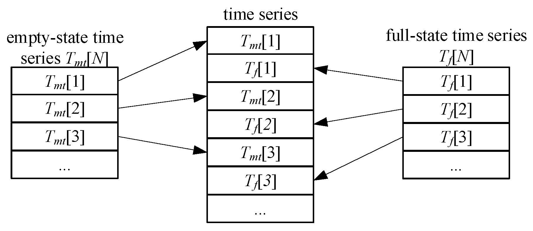
T_f and T_mt are both discrete random variables, and these two are mutually independent.

(2)

T_f and T_mt alternate in the duration sequence.

Then, the PPS state sequence can be generated through two following procedures: ① Random variables T_f and T_mt generate time series {T_f[N]} and {T_mt[N]} of length N from their respective probability distributions, the two of which are interleaved as shown in Figure 1. ② Each element in the resulting sequence represents the number of consecutive occurrences of full or empty values. Specifically, T_f[K] and T_mt[K] indicate the full value of consecutive times of T_f[K] and the empty value of consecutive times of T_mt[K], respectively. Assigning ‘1’ to full states and ‘0’ to empty states yields the binary PPS sequence illustrated in Figure 2.

Applying theories of probability and statistics, we derive the expectation, frequency, and state probabilities of the PPS state random variables T_f and T_mt.

$$\left\{\begin{array}{l}{N}_{\mathrm{f}}=N\times E\left\{T_{\mathrm{f}}\right\}\\ N_{\mathrm{mt}}=N\times E\left\{T_{\mathrm{mt}}\right\}\end{array}\right.,$$

(3)

$$\left\{\begin{array}{l}{P}_{\mathrm{f}}={\displaystyle \frac{N_{\mathrm{f}}}{N_{\mathrm{f}}+N_{\mathrm{mt}}}}={\displaystyle \frac{E\left\{T_{\mathrm{f}}\right\}}{E\left\{T_{\mathrm{f}}\right\}+E\left\{T_{\mathrm{mt}}\right\}}}\\ P_{\mathrm{mt}}={\displaystyle \frac{N_{\mathrm{mt}}}{N_{\mathrm{f}}+N_{\mathrm{mt}}}}={\displaystyle \frac{E\left\{T_{\mathrm{mt}}\right\}}{E\left\{T_{\mathrm{f}}\right\}+E\left\{T_{\mathrm{mt}}\right\}}}\end{array}\right.,$$

(4)

where N_f denotes the total frequency of full states, N_mt denotes the total frequency of empty states, E{•} denotes the expectation of a random variable, and P_f and P_mt are the probabilities of PPS signals in the full and empty states, respectively.

By the Law of Large Numbers, the sample mean converges to the random variable’s expectation as the sample size approaches infinity.

$$\left\{\begin{array}{l}{T}_{\mathrm{f},\mathrm{avg}}=E\left\{T_{\mathrm{f}}\right\}\\ T_{\mathrm{mt},\mathrm{avg}}=E\left\{T_{\mathrm{mt}}\right\}\end{array}\right.,$$

(5)

where T_f,avg denotes the sample mean of T_f, and T_mt,avg denotes the sample mean of T_mt. Substituting Equation (5) into Equation (4), we obtain

$$\left\{\begin{array}{l}{P}_{\mathrm{f}}={\displaystyle \frac{T_{\mathrm{f},\mathrm{avg}}}{T_{\mathrm{f},\mathrm{avg}}+T_{\mathrm{mt},\mathrm{avg}}}}\\ P_{\mathrm{mt}}={\displaystyle \frac{T_{\mathrm{mt},\mathrm{avg}}}{T_{\mathrm{f},\mathrm{avg}}+T_{\mathrm{mt},\mathrm{avg}}}}\end{array}\right.,$$

(6)

As can be seen, when the sample size is sufficiently large, cross-combining random variables T_f and T_mt to form the PPS state sequence still preserves the total frequency of full and empty values in the PPS signal. Consequently, the PPS state model is theoretically compliant with the population frequency distribution requirements.

2.2. Clock Synchronization Algorithm

2.2.1. Virtual Clock

Although actual crystal oscillators demonstrate nonlinear behavior, their short-term stability exhibits minimal deviations. Herein, the state-space equation of the local clock is referred to as a virtual clock. The linear virtual clock is proposed to approximate the dynamic relationship between the local clock’s frequency offset and phase offset.

$$\left\{\begin{array}{l}R(k)=h{(k)}^T\theta (k)\\ \theta (k)={\left[\begin{array}{cc}\alpha (k)& \beta (k)\end{array}\right]}^T\\ h(k)={\left[\begin{array}{cc}C(k)& 1\end{array}\right]}^T\end{array}\right.$$

(7)

where k denotes the number of algorithm steps; α(k) denotes the frequency correction coefficient; β(k) denotes the phase correction coefficient; θ(k) denotes the parameter vector of the local clock model; and h(k) denotes the observation data vector of the local clock model.

Using the random walk model for θ(k) as the system equation and the linear model in Equation (7) as the observation equation, we establish the discrete-time state-space equation given in Equation (8).

$$\left\{\begin{array}{l}\theta (k+1)=I \theta (k)+\omega (k)\\ R(k)=h{(k)}^T\theta (k)+\upsilon (k)\end{array}\right.,$$

(8)

where υ(k) denotes the observed noise; ω(k) denotes the system noise; and I denotes the identity matrix. Let Q and V denote the covariance matrices of the system noise and observation noise, respectively, satisfying

$$\left\{\begin{array}{l}Q=E\left[\omega (k)\omega {(k)}^T\right]=\left[\begin{array}{cc}{\mu }^2& 0\\ 0& {\sigma }^2\end{array}\right]\\ V=E\left(\upsilon {\upsilon }^T\right)={\lambda }^2\end{array}\right.,$$

(9)

where μ² denotes the covariance of the frequency noise; σ² denotes the covariance of the phase noise; and λ² denotes the covariance of the observation noise. Generally, the process noise covariance of phase noise is marginally higher than that of frequency noise [19]. Herein, the covariance matrix Q in the Kalman filter is given by

$$Q=c\cdot \left[\begin{array}{cc}1\times {10}^{-4}& 0\\ 0& 1\end{array}\right]=c{Q}_0,$$

(10)

where Q₀ denotes the base matrix Q used to constrain the relative magnitudes of phase noise and frequency noise. c is a real constant.

2.2.2. Parameter Estimation

The Kalman Filter (KF) algorithm iteratively estimates the parameters of the virtual clock [20].

(1)

Parameter initialization

$$\left\{\begin{array}{l}\widehat{\theta }(0|0)=\theta (0)\\ P(0|0)=P(0)\end{array}\right.,$$

(11)

(2)

Prediction stage

$$\left\{\begin{array}{l}\widehat{\theta }(k+1|k)=\widehat{\theta }(k|k)\\ P(k+1|k)=P(k|k)+Q\end{array}\right.,$$

(12)

(3)

Renewing the gain matrix

$$K(k+1)=P(k+1|k)h(k){[h{(k)}^{T}P(k+1|k)h(k)+R]}^{-1},$$

(13)

(4)

Renewing model parameters

$$\left\{\begin{array}{l}\epsilon (k+1)=R(k+1)-h{(k)}^T\widehat{\theta }(k+1|k)\\ \widehat{\theta }(k+1|k+1)=\widehat{\theta }(k|k)+K(k+1)\epsilon (k+1)\end{array}\right.,$$

(14)

(5)

Renewing the matrix P

$$P(k+1|k+1)=[I-K(k+1)h{(k)}^T]P(k+1|k),$$

(15)

The execution process of this KF algorithm is stated as follows: First, the parameters θ and covariance matrix P are initialized, where the initial value settings directly affect the algorithm’s convergence speed. Second, the current state estimate at time k is used to predict parameters θ and matrix P at time k + 1. Subsequently, the Kalman gain matrix K is computed based on this predicted covariance matrix P. Then, the parameters θ and matrix P are predicted at the step k + 1 according to the observed reference time and gain matrix. Finally, the iterative process continuously refines the model parameters in real time.

2.2.3. Self-Compensation Algorithm

To mitigate timing inaccuracies caused by random GNSS PPS signal loss, a time synchronization compensation algorithm is presented in Figure 3. This solution uses the PPS signal as an interrupt trigger and operates periodically. First, PPS interrupts trigger the acquisition, sampling, and caching of local and reference time. Then, the algorithm determines the PPS signal state (empty or full) based on whether a valid reference time is captured. When the PPS signal is in an empty state, the virtual clock in Equation (7) is used to predict and compensate for the reference time. After that, the local time and reference time are applied to the KF algorithm to estimate the virtual clock’s frequency deviation and phase deviation.

The validity of the signal should be verified prior to estimating model parameters. Theoretically, predictive compensation for empty-state signals can fill in the loss of GNSS reference time. Notably, this algorithm disregards the impact of GNSS reference time loss on PSS signal accuracy. During the PPS signal interruption handling, the local time and reference time are captured simultaneously. Prior to the initial execution of the compensation algorithm, valid time synchronization must be established to align local time with reference time, facilitating rapid algorithm convergence. Furthermore, to minimize the impact of PPS signal interruptions on other program processes, local clock data acquisition is performed exclusively in the PPS hard interrupt routine in Figure 3, while the data processing is carried out in the algorithm’s main program.

3. Experimental

3.1. Experimental Platform

The circuit board of an experimental V2X terminal is shown in Figure 4. This terminal is integrated with a 5G communication module, enabling information exchange with other V2X terminals via V2X interface functions. Through an auxiliary chip expanded via the SPI interface, the terminal communicates with the in-vehicle CAN network and supports program debugging through one USB port. The terminal also incorporates two clock sources: a quartz crystal oscillator and a GNSS receiver. The crystal oscillator circuit generates high-frequency pulse signals, while the GNSS receiver provides reference time and PPS signals as the primary clock source.

The communication module’s CPU runs a Linux real-time operating system. The synchronization algorithm is responsible for acquiring the local time and reference time corresponding to the local clock and reference clock, respectively. The ‘gettimeofday()’ function is called to retrieve the local time provided by the crystal oscillator circuit, returning the time elapsed since 1 January 1970 with a resolution of 1 microsecond (μs). The GNSS receiver generates the PPS signal and reference time at whole-second intervals. Specifically, the PPS signal is delivered directly to the communication module via GPIO pins, while the reference time is parsed by the auxiliary chip before being transmitted to the communication module.

3.2. Data Acquisition

Exploiting the nanosecond-level precision and whole-second output characteristics of the PPS signal, a clock sampling scheme is designed, as illustrated in Figure 5. The data acquisition program is executed periodically in response to the triggering of the PPS signal. When the PPS signal generates a rising edge, it triggers a hardware interrupt in the communication module, prompting the acquisition program to immediately read the local time information. Upon completion, the program switches to the interrupt context to continue execution. During the interrupt service, the program waits for the reference time to be transmitted via the SPI interface. If the routine fails to receive the reference time within the preset time window, the reference time retains its last received value, and the current PPS status is marked as ‘empty’. Conversely, if the reference time is successfully received, it is updated to the latest value, and the PPS status is marked as ‘full’. Upon completing data reception, the collected data are stored in external memory in a timestamp format that includes the PPS interrupt count, PPS status, local time, and reference time, persisting until the main clock synchronization algorithm routine terminates.

In the above scheme, local time acquisition should be performed within the PPS interrupt service routine (ISR) to minimize the impact of Linux system scheduling and multithreading on function call latency, which is considered negligible in this context. Although the reference time is processed in the ISR, this approach avoids the delays associated with parsing the reference time and SPI transmission. Furthermore, since the reference time always corresponds to the PPS signal trigger moment, the introduced latency only results in a delay in data storage, while the captured local time and reference time remain synchronized to the same temporal instance. Experimental measurements indicate that the communication module experiences a latency of approximately 200 milliseconds (ms) when receiving the reference time. This latency not only ensures sufficient time for data storage to complete in one second, but also prevents access conflicts between the PPS ISR response and the reference time reception process.

Three V2X terminals incorporating the proposed algorithm were sequentially labeled as D1, D2, and D3. These terminals were set up in Room 203, Building 7, at No. 16 Lengquan East Road, Haidian District, Beijing, with their GNSS antennas connected outdoors. All three terminals were initialized simultaneously within the same time window. Following the initial synchronization of each terminal’s local time to the reference time, they operated continuously for 4 h, generating a total of 144,000 sets of sampling data per terminal.

4. Results and Discussion

4.1. Clock Model Performance Analysis

4.1.1. Virtual Clock Performance Analysis

Parameter estimation for polynomial models of orders 1 to 7 was conducted for the three terminal groups using the principle of least squares. Herein, the pseudo-code for the LS algorithm is listed in

Table 1. The pseudo-code for parameter estimation of the least squares.

Input:  x: Reference time array  y: Local time array  deg: Polynomial order Output:  θ: Parameter
1:	For i in range(length(x)) do
2:	V[i,0] $\leftarrow$x[i]
3:	V[i,1] $\leftarrow$1
4:	end
5:	U, S, VT $\leftarrow$svd(V)
6:	threshold $\leftarrow$max(len(x), deg + 1) * max(S) * accuracy
7:	for s in S do
8:	If s > threshold
9:	then s_inv $\leftarrow$1/s
10:	else s_inv $\leftarrow$0
11:	end
12:	θ$\leftarrow$VTT * diag(S_inv) * UT * y
13:	Return θ

. The deviations between the models and the measured data were statistically analyzed, and the mean deviations and standard deviations of the three terminal groups are summarized in

Table 2. Average bias of local clock models of three terminals.

Model Order	1st	2nd	3rd	4th	7th
mean value/10−6 µs	2.865	3.659	1.648	1.192	5.316
standard deviation/µs	77.745	49.854	38.884	30.416	18.428

. The mean deviation of the models does not exhibit a clear trend with increasing model order. Among them, the fourth-order model achieves the lowest mean deviation of approximately 1 × 10⁻⁶ μs, while the seventh-order model shows the highest mean deviation of about 5 × 10⁻⁶ μs, approximately 4.5 times that of the fourth-order model. In contrast, their standard deviations demonstrate a decreasing trend as the model order increases. When the model order increases from 1 to 7, the standard deviation decreases from 78 μs to 18 μs, representing a reduction of 76.9%.

Higher-order polynomials exhibit lower model standard deviations, and their model data closely approximates the actual measurements. However, increased model order also implies greater modeling complexity. To balance the deviation and complexity of models, the fourth-order polynomial is selected to capture the nonlinear characteristics of the local clock. The corresponding model parameters for the three terminals are listed in

Table 3. Fourth-order model parameters of local clocks.

nth-Order Coefficient	D1	D2	D3
4	−9.62 × 10−20	−1.28 × 10−19	−1.28 × 10−19
3	1.82 × 10−15	3.62 × 10−15	3.33 × 10−15
2	−6.82 × 10−12	−3.82 × 10−11	−3.00 × 10−11
1	0.999999588	0.999999057	0.99999926
0	9.62 × 10−5	3.05 × 10−5	9.35 × 10−5

.

Notably, the first-order coefficients of all three terminals are significantly greater than higher-order terms, and the absolute values of the coefficients decrease with increasing polynomial order. This indicates that the nonlinear characteristics of local clocks are predominantly captured by the lower-order terms. At the same time, this observation supports the validity of using linear approximations for local clock models in time synchronization algorithms, as they broadly reflect the actual clock behavior.

4.1.2. PPS Model Performance Analysis

Based on the measured data from three terminals, the statistical characteristics of empty states, full states, and their respective durations during the reference time are analyzed. The results are summarized in

Table 4. Frequency statistics of PPS states for 4 h field-measured three terminals.

Statistical Quantity	Total Counts	Mean Counts	Frequency
empty	2831	943.67	0.0655
full	40,369	13,456.33	0.9345

and

Table 5. Duration statistic results of PPS states.

Statistical Quantity	Mean Value	Standard Deviation	Maximum Value	Minimum Value
empty-state duration/s	1.074	0.310	7	1
full-state duration/s	15.259	14.739	112	1

. In terms of total frequency, the PPS signal predominantly remains in the full state (93.45%), while the empty state occurs for only 6.55% of the time. In terms of duration, the empty state has a mean duration of 1.074 seconds (s) with a standard deviation of 0.310 s, whereas the full state exhibits a mean duration of 15.259 s and a standard deviation of 14.739 s. This finding indicates that the full state occurs with significantly higher probability than the empty state, reflecting a low likelihood of reference time loss. The relatively small standard deviation in the duration of the empty state suggests that its occurrences are consistent and concentrated. In contrast, the full state exhibits a relatively high standard deviation in duration, indicating greater variability and dispersion in its occurrence patterns.

The distribution of empty-state durations is shown in Figure 6. As illustrated, the empty-state durations are predominantly concentrated at 1 s, accounting for 93.43% of all samples. A duration of 2 s accounts for 5.96% of the total, while all other durations combined represent only 0.61%. Applying principles of probability and statistical theory, the empty-state duration is modeled as a discrete random variable, with the observed sample frequencies closely approximating their corresponding probabilities. The resulting probability distribution is summarized in

Table 6. Probability distribution of empty value time.

Duration/s	1	2	3	4	7
occurrence count	2462	157	12	3	1
frequency	0.9343	0.0596	0.0046	0.0011	0.0004

.

The distribution of full-state durations is shown in Figure 7. The durations span a wide range from a minimum value of 1 s to a maximum value of 112 s, with shorter durations occurring more frequently. During data processing, we experimented with fitting results of various probability distributions, such as the exponential, gamma, log-normal, and chi-squared distributions, and evaluated the goodness of fit for each distribution using the sum of squared errors (SSE) metric, as listed in

Table 7. Errors of different distribution models.

Distribution Model	SSE	p-Value
Gamma	0.078939	0.466
Chi-squared	0.058494	0.032
Exponential	0.003487	0.364
Log-normal	0.004713	0.187

.

In the aforementioned table, a smaller value of the SSE indicates that the fitted curve is closer to the actual data points. The exponential distribution has the smallest SSE, equal to 0.003487, suggesting that its fitted curve is closest to the data points in the least squares sense. Meanwhile, the chi-squared test is used to evaluate the difference between the frequency distribution of observed data and the hypothesized theoretical distribution. A larger p-value implies a less significant difference. Although the p-value of the gamma distribution is 0.466, slightly larger than that of the exponential distribution, the gamma distribution exhibits the largest SSE, equal to 0.078939. Using the full-value duration data for the chi-squared test, the calculated p-value is approximately 0.364, which is greater than the threshold of 0.05, so the null hypothesis is accepted. Therefore, the exponential distribution is selected as the PPS distribution model.

After offset adjustment and normalization, the probability density of full-state durations is found to follow an exponential distribution, as described by Equation (16).

$$P_f(t_{cs})=\frac{1}{14.2591}{e}^{-\frac{t_{cs}-1}{14.2591}},\hspace{0.33em}{t}_{cs}\ge 1$$

(16)

where P_f(t) is the probability density function of the full-state duration, and t_cs denotes the duration.

4.2. Algorithm Performance Analysis

4.2.1. Influence of Noise on Algorithm Convergence

Simulated data are generated by superimposing Gaussian noise with varying standard deviations onto the established clock model. The data are used to analyze the time synchronization deviation of the KF algorithm under different noise levels. For example, the synchronization deviation curve for terminal D2 is shown in Figure 8, with corresponding statistical results presented in

Table 8. Time synchronization bias affected by different noises.

Noise Levels/μs	100	10	1
mean value/μs	0.744	0.688	0.697
standard deviation/μs	102.319	10.291	1.103

. At three noise levels (1 μs, 10 μs, and 100 μs), the terminal’s synchronization deviation converges rapidly and stabilizes within distinct numerical ranges. As the noise standard deviation increases, the fluctuation ranges expand, resulting in intervals of −3 to 5 μs, −38 to 45 μs, and −381 to 351 μs, respectively. Simulation results demonstrate that the convergence of the KF synchronization algorithm remains robust to Gaussian noise, maintaining stable performance across various noise environments.

4.2.2. Performance Comparison

By combining clock model data superimposed with Gaussian noise (with a standard deviation of 10 μs) and the state sequence generated by the PPS model, simulated sequence data incorporating random loss of GNSS PPS signals is generated. This dataset enables a comparative evaluation of the time synchronization performance of the KF algorithm and the least squares (LS) algorithm.

For example, the time synchronization deviation curves based on the terminal D2 model are shown in Figure 9, with the corresponding statistical results summarized in

Table 9. Time synchronization bias from different algorithms.

Algorithm	LS	KF
mean value/µs	−0.365	0.070
standard deviation/µs	13.952	10.420

. After 4 h of operation, the original deviation of the local clock increases to 6.0 ms. Both the LS and KF algorithms exhibit convergent behavior. However, their synchronization deviations differ significantly. Notably, the steady-state fluctuation range of the LS algorithm spans from −51.7 to 60.3 μs, whereas the KF algorithm achieves a narrower and more symmetric range of −40.6 to 40.4 μs. This represents an improvement of −11.1 to 19.9 μs compared to the LS algorithm. In terms of statistical metrics, the mean deviation of the KF algorithm is 0.07 μs, which is less than 20% of the corresponding value for the LS algorithm. The standard deviation of the KF algorithm is 10.4 μs, 3.6 μs smaller than that of the LS algorithm. These simulation results confirm that the KF algorithm achieves significantly smaller prediction deviations compared to the LS algorithm.

4.2.3. Real-Time Verification

The consistent KF algorithm was implemented and executed across three terminals. The measured synchronization deviation curves are illustrated in Figure 10, with corresponding statistical results presented in

Table 10. Time synchronization bias of the field-measured three terminals.

Terminals	D1	D2	D3
mean value/µs	0.326	0.198	−1.079
standard deviation/µs	13.136	15.811	13.093

.

The original synchronization deviations of the local clocks for all three terminals exhibit a nonlinear, monotonically increasing trend over time. After 4 h of operation, the original deviations for terminals D1, D2, and D3 reach 7.3 ms, 5.4 ms, and 14.4 ms, respectively. Following the application of the KF algorithm, the corrected synchronization deviation curves converge and become nearly flat, indicating effective compensation for clock drift. The mean synchronization deviations for terminals D1, D2, and D3 are −1.1 μs, 0.3 μs, and 0.2 μs, respectively, with corresponding standard deviations of 13.1 μs, 13.1 μs, and 15.8 μs. Experimental results demonstrate that the KF algorithm performs stably in the three terminals, significantly reducing synchronization deviations from the millisecond to microsecond level compared to the original, uncorrected deviations.

4.3. Discussion

In a Cartesian coordinate system, the geometric model of an ideal clock is represented by a straight line with unit slope passing through the origin. However, due to the frequency drift inherent in practical clocks, phase deviations arise between clocks, resulting in temporal misalignments. The clock offset model characterizes the discrepancy between a real clock and an ideal reference clock. It can be classified into four main types: the phase offset model, the linear model, the incremental linear model, and the higher-order polynomial model [21]. Specifically, higher-order models incorporate the dynamic behavior of clock drift, offering improved accuracy in modeling real-world clock performance, albeit with greater computational demands.

Given the variations in mean and variance trends across different clock models, a composite performance metric is developed by incorporating weighted means and variances to assess the overall model accuracy.

$$R_n=\alpha {\displaystyle \frac{M_n}{{\displaystyle \sum _i{M}_i}}}+\left(1-\alpha \right){\displaystyle \frac{S_n}{{\displaystyle \sum _i{S}_i}}}$$

(17)

where n denotes the model order; i represents the orders 1, 2, 3, 4, and 7; M_n is the device-averaged mean of the bias for the n-th order model; S_n is the device-averaged variance of the bias for the n-th order model; α is the weight coefficient, with a value ranging from 0 to 1; and R_n is the comprehensive performance indicator for the n-th order model. A smaller R_n indicates better model performance.

Based on Equation (17), the computed R_n values for the 1st-, 2nd-, 3rd-, 4th-, and 7th-order clock models are 0.295, 0.239, 0.153, 0.117, and 0.196, respectively. Consequently, the fourth-order model, exhibiting the minimum composite performance index, is chosen to represent the temporal characteristics of the device’s local clock.

To evaluate the performance of the PPS model, 1000 simulation samples were generated using the probabilistic model, resulting in a total time duration of approximately 4 h. The occurrences of full-value events, empty-value events, and their respective durations were recorded and summarized in

Table 11. PPS model performance data compared with measurement data.

Samples	Full-Value Events		Empty-Value Events
	Durations (s)	Frequency	Durations (s)	Frequency
simulations	15.248	0.9341	1.07433	0.0659
measurements	15.259	0.9345	1.07438	0.0655

. Compared with the measured data, the mean differences in the durations of full-value and empty-value events are −0.011 s and −0.0005 s, respectively, indicating that the state sequences of the PPS simulation samples well preserve the original duration distribution. Meanwhile, the frequency differences for full-value and empty-value events are −0.0004 and 0.0004, respectively, indicating that the state sequence of the PPS simulation samples can reproduce the original signal states with high accuracy.

The validation results demonstrate that the probabilistic models for full-value and empty-value events are reliable, and the theoretical model, based on reasonable and justifiable assumptions, effectively characterizes PPS signals under conditions of either GNSS signal loss or parsing failure. The GNSS signal loss may result from blocking objects, and its duration depends on the types and volumes of blocking objects. Although the model parameters and probability density may vary across different environments, this modeling methodology remains generalizable.

To enable synchronization with the GNSS reference time, a KF-based iterative algorithm was established for estimating the parameters of the virtual clock model in V2X communication terminals by using the models of local clocks and PPS. In comparison with the LS batch processing algorithm, the KF algorithm features reduced data storage requirements and improved real-time capability. However, the performance of the KF algorithm is affected by the initial values, system noise, and measurement noise. The algorithm convergence becomes faster as the model parameters θ approach their theoretical true values. A larger norm of the P matrix corresponds to a faster convergence rate of the algorithm. Therefore, appropriate system noise and measurement noise matrices were determined through simulation analysis. The Kalman Filter (KF) algorithm was then optimized with the following parameters: P = I × 10⁵, θ = [0, 1]’, c = 1, and R = 0.5.

In contrast to conventional GNSSDO and multi-GNSS methods, the proposed time synchronization approach is hardware-independent, lower in cost, and more convenient to deploy. Experimental results show that the proposed clock synchronization method significantly improves synchronization accuracy, reducing the mean synchronization offset to 1 µs, while maintaining a standard deviation of around 10 µs, which demonstrates both high precision and stability. Although the proposed method achieves an accuracy that is slightly lower than that of the GNSSDO method (0.356 µs) and the multi-GNSS method (2 µs), the achieved accuracy satisfies the stringent time synchronization requirements for safety control systems in ICVs, which require precision within 100 µs. Furthermore, the proposed clock correction algorithm improves the system’s ability to maintain synchronization in the presence of faults or disturbances through integrated software modules.

Although the proposed algorithm was evaluated in a single outdoor environment, its reliability under varying conditions, such as in the presence of obstructions or temperature fluctuations, should also be investigated. Nevertheless, the model-driven time synchronization approach presented in this work demonstrates general applicability in terms of theoretical formulation and algorithm design. Next step, this work can conduct experiments in diverse environments and perform long-term testing to further validate the reliability of the algorithm.

5. Conclusions

When intelligent connected vehicles (ICVs) operate near high-rise buildings, under overpasses, or within tunnels, the onboard GNSS PPS signals are prone to degradation or loss. To address time synchronization instability in V2X terminals of ICVs caused by random GNSS PPS signal loss, this paper proposes a model-based design for a local clock synchronization algorithm.

The PPS sequence model, based on probability and statistics, is investigated to accelerate the development of local clock correction algorithms for onboard terminals. This model assumes that the durations of the full and empty states are mutually independent random variables. Through theoretical derivation, simulations, and empirical data analysis, the results demonstrate that the active state duration follows an exponential distribution, while the inactive state duration is characterized as a finite discrete random variable with bounded values. Subsequently, a fourth-order polynomial clock model is developed for the terminal. Its first-order derivative is employed to construct a state-space representation of the time synchronization process. The Kalman Filter (KF) algorithm then identifies model parameters, enabling prediction and compensation for lost reference signals. This achieves precise time synchronization in V2X terminals.

The stability of the KF algorithm is robust to variations in noise standard deviation. Specifically, the mean synchronization deviation persists below 1 μs. Under random PPS signal loss, the KF algorithm demonstrates superior performance compared to the Least Squares (LS) algorithm, exhibiting lower values in mean deviation, standard deviation, and data fluctuation range. The proposed algorithm was subsequently embedded and implemented on three terminal devices. Experimental results obtained after 4 h of operation confirm its stable performance across all three units. The absolute time synchronization deviations remain below 1.1 μs, with the standard deviations consistently under 16 μs.

In contrast to the backup clock source method for time synchronization, the approach of establishing a virtual clock to compensate for random PPS signal loss requires only additional software modules, eliminating the need for extra hardware. In scenarios of random GNSS signal loss, this method enables terminals to maintain microsecond-level time synchronization accuracy while demonstrating strong real-time performance. Consequently, it proves highly applicable across diverse V2X terminals equipped with GNSS receivers. Future research will focus on an in-vehicle performance evaluation of the algorithm.

References

1. Solaas, J.V.; Mariconti, E.; Tuptuk, N. Systematic Literature Review: Anomaly Detection in Connected and Autonomous Vehicles. IEEE Trans. Intell. Transp. Syst. 2025, 26, 43–57. [Google Scholar] [CrossRef]
2. Li, J.; Fotouhi, A.; Liu, Y.G. Review on Eco-driving Control for Connected and Automated Vehicles. Renew. Sust. Energy Rev. 2024, 189, 114025. [Google Scholar] [CrossRef]
3. Tavasoli, M.; Sarrafzadeh, A.; Khaleghi, M. Data Communication Challenges of Connected and Automated Vehicles in Rural Areas. IEEE Access 2025, 13, 29220–29251. [Google Scholar] [CrossRef]
4. Chen, S.Z. Critical Thinking and Suggestions on C-V2X with the Developments of Intelligent Connected Vehicles. Telecommun. Sci. 2022, 38, 1–24. [Google Scholar]
5. Ansere, J.A.; Han, G.; Wang, H. A Novel Reliable Adaptive Beacon Time Synchronization Algorithm for Large-Scale Vehicular Ad Hoc Networks. IEEE Trans. Veh. Technol. 2019, 68, 11565–11576. [Google Scholar] [CrossRef]
6. Li, M.; Ma, W.; Peng, Z. Skew Estimation for Clock Synchronization Without Timestamp Exchange Under Exponential Delays. IEEE Trans. Veh. Technol. 2023, 72, 16582–16591. [Google Scholar] [CrossRef]
7. Haider, S.; Abbas, G.; Abbas, Z.H. VLCS: A Novel Clock Synchronization Technique for TDMA-based MAC Protocols in VANETs. In Proceedings of the 2019 4th International Conference on Emerging Trends in Engineering, Sciences and Technology (ICEEST), Karachi, Pakistan, 10–11 December 2019. [Google Scholar] [CrossRef]
8. Medani, K.; Aliouat, M.; Aliouat, Z. Fault tolerant time synchronization using offsets table robust broadcasting protocol for vehicular ad hoc networks. AEU-Int. J. Electron. Commun. 2017, 81, 192–204. [Google Scholar] [CrossRef]
9. Shi, C.; Gu, S.F.; Lou, Y.D. Real-time wide-area precise positioning and precise timing service system. Acta Geod. Cartogr. Sin. 2022, 51, 1206–1214. [Google Scholar]
10. Jiao, W.H.; Zhang, H.J.; Zhu, L. Assessment method and analysis of GNSS broadcast coordinated universal time offset error. Acta Geod. Cartogr. Sin. 2020, 49, 805–815. [Google Scholar]
11. Grenier, A.; Lohan, E.S.; Ometov, A. A Survey on Low-Power GNSS. IEEE Commun. Surv. Tutor. 2023, 25, 1482–1509. [Google Scholar] [CrossRef]
12. Kim, W.; Seo, J. Low-Cost GNSS Simulators With Wireless Clock Synchronization for Indoor Positioning. IEEE Access 2023, 11, 55861–55874. [Google Scholar] [CrossRef]
13. Hasan, K.F.; Wang, C.; Feng, Y. Time synchronization in vehicular ad-hoc networks: A survey on theory and practice. Veh. Commun. 2018, 14, 39–51. [Google Scholar] [CrossRef]
14. Bauer, J.; Andrich, C.; Ihlow, A. Characterizing GPS Disciplined Oscillators for Distributed Vehicle-to-X Measurement Applications. In Proceedings of the 2020 Joint Conference of the IEEE International Frequency Control Symposium and International Symposium on Applications of Ferroelectrics (IFCS-ISAF), Keystone, CO, USA, 19–23 July 2020. [Google Scholar] [CrossRef]
15. Bui, Q.T.; Elango, A.; Landry, R. FPGA-Based Autonomous GPS-Disciplined Oscillators for Wireless Sensor Network Nodes. Sensors 2022, 22, 3135. [Google Scholar] [CrossRef] [PubMed]
16. Boehmer, T.J.; Bilén, S.G. Low-Power GPS-Disciplined Oscillator Module for Distributed Wireless Sensor Nodes. Electronics 2021, 10, 716. [Google Scholar] [CrossRef]
17. Hasan, K.F.; Feng, Y.; Tian, Y.C. Precise GNSS Time Synchronization with Experimental Validation in Vehicular Networks. IEEE Trans. Netw. Serv. Manag. 2023, 20, 3289–3301. [Google Scholar] [CrossRef]
18. Hasan, K.F.; Feng, Y.; Tian, Y.C. GNSS Time Synchronization in Vehicular Ad-Hoc Networks: Benefits and Feasibility. IEEE Trans. Intell. Transp. Syst. 2018, 19, 3915–3924. [Google Scholar] [CrossRef]
19. Xuan, X.; He, J.; Zhai, P. Kalman Filter Algorithm for Security of Network Clock Synchronization in Wireless Sensor Networks. Mob. Inf. Syst. 2022, 2022, 1–11. [Google Scholar] [CrossRef]
20. Phil, K. Kalman Filter for Beginners: With MATLAB Examples; CreateSpace Independent Publishing Platform: North Charleston, SC, USA, 2011; pp. 47–72. [Google Scholar]
21. Yiğitler, H.; Badihi, B.; Jäntti, R. Overview of Time Synchronization for IoT Deployments: Clock Discipline Algorithms and Protocols. Sensors 2020, 20, 5928. [Google Scholar] [CrossRef] [PubMed]
Figure 1. Signal time series.
Technologies 13 00273 g001
Figure 2. PPS State sequence.
Technologies 13 00273 g002
Figure 3. Time synchronization compensation algorithm.
Technologies 13 00273 g003
Figure 4. Onboard V2X smart terminals: (a) circuit board, (b) schematics.
Technologies 13 00273 g004
Figure 5. Data acquisition flow chart.
Technologies 13 00273 g005
Figure 6. Probability density of empty value time: time of duration tcs and probability density Pmt.
Technologies 13 00273 g006
Figure 7. Probability density of full value time: time of duration tcs and probability density Pf.
Technologies 13 00273 g007
Figure 8. Time synchronization bias curves of different noises.
Technologies 13 00273 g008
Figure 9. Time synchronization bias curves of different algorithms.
Technologies 13 00273 g009
Figure 10. Time synchronization bias curves of field-measured three terminals: (a) D1, (b) D2, (c) D3.
Technologies 13 00273 g010