Analysis of Surface Roughness and Machine Learning-Based Modeling in Dry Turning of Super Duplex Stainless Steel Using Textured Tools

Abstract

One of the most critical aspects of turning, and machining in general, is the surface roughness of the finished product, which directly influences the performance, functionality, and longevity of machined components. The accurate prediction of surface roughness is vital for enhancing component quality and machining efficiency. This study presents a machine learning-driven framework for modeling mean roughness depth (Rz) during the dry machining of super duplex stainless steel (SDSS 2507). SDSS 2507 is known for its exceptional mechanical strength and corrosion resistance, but it poses significant challenges in machinability. To address this, this study employs flank-face textured cutting tools to enhance machining performance. Experiments were designed using the L₂₇ orthogonal array with three continuous factors, cutting speed, feed rate, and depth of cut, and one categorical factor, tool texture type (dimple, groove, and wave), along with surface roughness as an output parameter. Gaussian Data Augmentation (GDA) was employed to enrich data variability and strengthen model generalization, resulting in the improved predictive performance of the machine learning models. MATLAB R2021a was employed for preprocessing, the normalization of datasets, and model development. Two models, Least-Squares Support Vector Machine (LSSVM) and Multi-Gene Genetic Programming (MGGP), were trained and evaluated on various statistical metrics. The results showed that both LSSVM and MGGP models learned well from the training data and accurately predicted Rz on the testing data, demonstrating their reliability and strong performance. Of the two models, LSSVM demonstrated superior performance, achieving a training accuracy of 98.14%, a coefficient of determination (R²) of 0.9959, and a root mean squared error (RMSE) of 0.1528. It also maintained strong generalization on the testing data, with 94.36% accuracy and 0.9391 R² and 0.6730 RMSE values. The high predictive accuracy of the LSSVM model highlights its potential for identifying optimal machining parameters and integrating into intelligent process control systems to enhance surface quality and efficiency in the complex machining of materials like SDSS.

1. Introduction

Manufacturing industries are vital to the global economy, serving as the backbone of production for essential components and products across sectors like automotive, aerospace, construction, and consumer electronics. Machining operations are critical in manufacturing, transforming raw materials into precise, intricate parts with high accuracy and versatility, essential for producing finished goods across various industries [1]. Discrete machining operations, such as turning, milling, and drilling, are extensively utilized in manufacturing industries to produce components with precise dimensions and requisite surface quality [2]. These processes are fundamental to machining, facilitating the production of complex geometries and ensuring the functional performance and reliability of machined components. Turning, a fundamental machining process, is notable for its extensive use in finishing operations, ensuring dimensional precision and superior surface quality [3].

Turning involves the removal of material from a rotating workpiece using a cutting tool to achieve the desired geometry and dimensions [4]. One of the most critical aspects of machining turning, and machining in general, is the surface roughness of the finished product, which serves as a critical indicator of quality [5,6]. Surface roughness directly influences the performance, functionality, and longevity of machined components [7]. Achieving the desired surface finish is challenging due to the complex interplay of process parameters, including cutting speed, feed rate, depth of cut, tool geometry, workpiece material properties, and external factors like machine dynamics and tool wear [6]. These parameters must be optimized to balance productivity, cost, and quality, a task that traditionally relies on operator expertise and can be time-consuming [1,4].

The importance of surface roughness extends beyond mere quality assurance; it also has economic implications. Manufacturing industries face substantial costs associated with monitoring and controlling surface roughness, including investments in advanced measurement equipment, personnel training, and time-intensive inspection processes [7]. Therefore, developing efficient and reliable predictive models for surface roughness is crucial to streamline production, reduce costs, and ensure consistent quality. Furthermore, in response to the growing demand for high-quality products and the challenges posed by complex machining processes, optimization methods have gained prominence in the manufacturing sector. These methods focus on modeling and predicting the effects of process parameters on machining outcomes, enabling manufacturers to achieve superior surface finishes and enhanced product functionality [4]. Given the complex, nonlinear interactions among machining parameters and their influence on surface finish, traditional empirical approaches often fall short in providing accurate predictions [8].

Over the past decade, the complexity and nonlinear nature of manufacturing processes have driven the adoption of machine learning (ML) techniques to enhance predictive modeling and optimization. ML approaches have gained significant popularity across engineering fields, offering robust capabilities for handling multi-variable interactions, responding efficiently system uncertainties, and uncovering hidden patterns within machining data. Their ability to deliver high prediction accuracy and enable real-time process adjustments has made them indispensable tools in advancing manufacturing efficiency, product quality, and sustainability. Motivated by these advantages, a growing body of research has successfully employed a wide range of ML models to predict machining responses such as surface roughness, cutting forces, and material removal rates, while also facilitating the optimization of process parameters across various materials and machining methods.

An extensive body of literature has been studied. A summary of the key findings on ML techniques employed for modeling and optimization approaches for various machining studies are presented in

Table 1. Summary of important past studies on machine learning implementation for modeling and optimization of machining.

Study	Material/Process	Modeling Techniques	Optimization Techniques	Key Inputs	Performance/ Outputs	Key Findings
Pimenov et al. [9]	Face milling of carbon steel 45 using coated carbide inserts	RF, MLP, RBF, Regression Trees	None (real-time prediction focus)	Tool wear, main drive power	Surface roughness	RF achieved highest accuracy; practical workshop application suggested
Yeganefar et al. [8]	Dry slot milling of 7075-T6 aluminum using coated inserts	ANN, SVM	NSGA-II	vc, fr, dc, tool type	Surface roughness, cutting forces	ANN-NSGA-II provided Pareto-optimal solutions; feed per tooth most influential
Gupta et al. [10]	Turning Ti alloy under MQL with nanofluids (NFs) using CBN tool	ANFIS, RSM	Coherence Distance Algorithm	vc, fr, approaching angle nanofluid type	Surface roughness, cutting force, temperature	Graphite NF most effective; ANFIS model superior; cutting speed/feed identified as critical factors
Zhang and Xu [4]	High-speed turning	GPR	None (prediction focus)	vc, fr, and dc	Cutting force, surface roughness, tool life	GPR provided high accuracy, stability, and robustness
Dubey et al. [6]	MQL turning of AISI 304 steel with nanofluids using carbide inserts	SVM, RF, Linear Regression	None (prediction focus)	vc, fr, and dc, cutting fluid type	Surface roughness	RF achieved best R2; highlighted ML’s potential in surface roughness prediction
Balonji et al. [11]	Dry milling of Al6061 using carbide inserts	ANN, ANFIS, ANN–PSO, ANN–GA, ANFIS–PSO, ANFIS–GA	PSO, GA (for hybrid models)	Spindle speed, vc and fr	Surface roughness	Hybrid models (ANFIS–GA) outperformed others; emphasized hyperparameter tuning
Kosarac et al. [12]	Milling of Ti-6Al-4V under different cooling conditions	RF, GB, Neural Networks	Taguchi design for initial parameter setting	vc, fr, and dc	Surface roughness	RF achieved highest accuracy; feed rate most influential
Dewangan et al. [13]	Dry turning of AISI 316 using carbide inserts	SVR, GPR, GBR	PSO	vc, fr, and dc	Surface roughness, Material Removal Rate (MRR)	GBR–PSO combination optimized efficiently the considered responses
Khlifi et al. [3]	Turning of AISI4340 using coated carbide insert	MLR, RFR, GBR, Bagging	None (focus on prediction)	vc, fr, and dc	Surface roughness, cutting force	RFR best for Ra; GBR best for force
Adizue and Takács [14]	Ultraprecision turning of AISI D2 steel using CBN insert	BRNN	Taguchi and Full Factorial DOE	vc, fr, and dc	Surface roughness, MRR	Full factorial design improved BRNN performance; Ra and MRR predicted accurately
Abbas et al. [15]	Dry precision turning of AISI 4340 steel using conventional and wiper inserts	XGBoost + MOORA	MOORA, PSO	vc, fr, dc and tool insert type	Surface roughness, MRR	Wiper inserts improved Ra; hybrid method highly effective
Reffas et al. [1]	Turning of cast iron using silicon nitride ceramic inserts	Dragonfly-optimized DNN, SVM	Ant Lion Optimizer, Desirability Function	vc, fr, dc and tool coating	Surface roughness, cutting force, pressure	hybrid ML and optimization improved efficiency and surface finish
May Tzuc et al. [16]	Heat gain prediction in flat naturally ventilated roofs	Multi-Gene Genetic Programming (MGGP)	None (focus on prediction)	Ambient air temperature, solar irradiation, wind speed, relative humidity, ventilated roof channel width	Heat flux	MGGP efficiently modeled the heat flux
Garg et al. [17]	Turning of AISI 1045 steel and 7075 Al alloy–15 wt% SiC composites	Ensemble-based (EN)-MGGP, MGGP	None (focus on prediction)	vc, fr, and dc	Surface roughness, tool life, power consumption	EN-MGGP outperformed MGGP in generalization; cutting speed had greatest impact on power consumption
Pawanr et al. [18]	Dry machining of Al6061 using carbide inserts	MGGP LSSVM Fuzzy-logic	None (focus on prediction)	vc, fr, dc, and nose radius	Power factor, energy efficiency, carbon emission	All ML methods effectively predicted the responses, with LS-SVM demonstrating the best performance

.

As outlined in Table 1, ML techniques have been extensively applied to model machining responses, predominantly based on cutting parameters. However, the use of Least-Squares Support Vector Machine (LSSVM) remains limited in this domain, despite its demonstrated effectiveness in handling high-dimensional data and delivering strong generalization performance, particularly with small datasets. Similarly, Multi-Gene Genetic Programming (MGGP), which offers the advantage of generating explicit analytical expressions and enhanced model interpretability, has seen only limited application in machining research. Moreover, while the surface texturing of cutting tools is increasingly recognized as a promising strategy for enhancing cutting performance and promoting sustainable machining, there remains a notable lack of studies leveraging machine learning for predicting surface roughness in the context of textured tooling.

Overall, the reviewed literature emphasizes the growing importance and success of machine learning approaches in modeling various machining processes. Across different materials, machining methods, and performance metrics such as surface roughness, cutting forces, and material removal rates, ML models such as Random Forest, Gradient Boosting, Support Vector Machines, Gaussian Processes, and Neural Networks have consistently demonstrated high prediction accuracy and practical applicability.

In view of the material-specific challenges and leveraging insights from the literature, this study, for the first time to the best of the authors’ knowledge, presents a machine learning-driven framework for modeling surface roughness obtained during the dry machining of super duplex stainless steel (SDSS 2507) with the use of flank-face textured cutting tools. The use of textured tools was motivated by their demonstrated benefits in improving machining performance [19,20]. The surface texturing of cutting tools has emerged as a promising strategy to mitigate machining challenges by modifying the tool–chip interface to reduce friction and improve tribological behavior. Gaussian Data Augmentation (GDA) was employed to enrich data variability and strengthen model generalization, resulting in improved predictive performance of the machine learning models.

In the present study, the original dataset, consisting of 27 experimental runs, based on the Taguchi L₂₇ fractional orthogonal array, was expanded to 81 samples through GDA. The machine learning techniques employed were Least Square Support Vector Machine (LSSVM) and Multi-Gene Genetic Programming (MGGP). Least-Squares Support Vector Machine (LSSVM) is a supervised learning method that adapts the principles of traditional Support Vector Machines (SVMs) by using a least-squares loss function. It minimizes a cost function that balances model complexity and error minimization through a regularization parameter. SVM and LSSVM have demonstrated successful applications in a variety of machining studies such as for predicting surface roughness [1,6,13], cutting forces [8], and energy efficiency [18]. It is especially effective when working with small to medium-sized datasets in high-dimensional feature spaces [19]. Its robustness against noisy data and strong generalization capability makes it a suitable choice for modeling complex machining phenomena [19]. Conversely, Multi-Gene Genetic Programming (MGGP), an advanced form of traditional Genetic Programming (GP), enhances symbolic regression by enabling the use of multiple genes within a single model [18]. These genes are linearly combined to produce the final output, allowing MGGP to generate interpretable and adaptable models. In the domain of machining, MGGP has been effectively applied to model surface finish [17], heat flux [16], energy efficiency [18], etc.

Having a strong motivation from the demonstrated benefits of texture-assisted machining and the increasing application of machine learning in manufacturing, this research aims to

• Develop predictive models for surface roughness using advanced ML techniques;
• Improve model robustness through data augmentation strategies tailored for small-scale machining datasets.

The models’ performance was thoroughly evaluated on both training and testing datasets to ensure their reliability and generalization capability. The findings aim to contribute to intelligent process control and the enhanced machinability of SDSS components, addressing existing gaps in both performance optimization and predictive modeling in the current research landscape. Figure 1 illustrates the overall methodology with the sequence of tasks performed in the present research work.

2. Overview of Modeling Techniques

2.1. Least-Squares Support Vector Regression

Least-Squares Support Vector Machine (LSSVM) is a regression that adapts the principles of Support Vector Machines (SVMs) to solve regression problems using a least-squares cost function. LSSVM aims to minimize a cost function that balances model complexity and error minimization [20]. This results in an efficient and flexible framework for predictive modeling.

In the context of regression, LSSVM aims to learn a function $f\left(x\right)$ that maps input vectors $x$ to the corresponding output $y$. The function $f\left(x\right)$ is given by Equation (1) [21]:

$$f\left(x\right)=w^T\phi \left(x\right)+b$$

(1)

where $w$ is the weight vector, $b$ is the bias term, and $\phi \left(x\right)$ is a mapping that projects the input $x$ into a higher-dimensional feature space, performed indirectly using a kernel function. The objective in LSSVM is to minimize a cost function, which combines a regularization term ${\displaystyle \frac{1}{2}}{\left|\left|w\right|\right|}^2$, controlling model complexity, and a least-squares loss function ${\displaystyle \frac{\gamma }{2}} {\sum }_{i=1}^N{\epsilon }_i^2$, penalizing the squared deviations ${\epsilon }_i$ (errors between predicted and true outputs). The overall cost function can be expressed as shown in Equation (2) [21]:

$$J\left(w, b, \left\{{\epsilon }_i\right\}\right)={\displaystyle \frac{1}{2}}{\left|\left|w\right|\right|}^2+{\displaystyle \frac{\gamma }{2}} {\sum }_{i=1}^N{\epsilon }_i^2$$

(2)

where γ is a regularization parameter that balances the trade-off between fitting the data and maintaining a simple model. The errors ${\epsilon }_i$ are the slack variables representing deviations between the predicted outputs and the actual target values.

Given a set of training data ${\left\{\left(x_i, y_i\right)\right\}}_{i=1}^N$, the LSSVM regression model aims to minimize the cost function while satisfying the following constraints: $y_i-f\left(x_i\right)={\epsilon }_i$, for each training example $i=1, ..., N$.

The resulting optimization problem is a convex quadratic programming problem, which is solved to determine the optimal model parameters $w$ and $b$.

To handle nonlinear regression tasks, LSSVM employs the kernel function. Instead of directly mapping the inputs to a high-dimensional feature space, LSSVM uses a kernel function $K(x, x\prime )$ to compute the inner product in that space. Common kernel functions include the radial basis function (RBF) kernel as shown in Equation (3):

$$K(x, x\prime )=exp\left(-{\displaystyle \frac{{\left|\left|x-x^{\prime }\right|\right|}^2}{2{\sigma }^2}}\right)$$

(3)

and the Polynomial kernel:

$$K(x, x\prime )={\left(1+x^T{x}^{\prime }\right)}^d$$

where $\sigma$ and $d$ are kernel parameters. Figure 2 presents the outline of the LSSVM model.

2.2. Multi-Gene Genetic Programming

Multi-Gene Genetic Programming (MGGP) is an evolutionary machine learning technique that extends traditional Genetic Programming (GP) by representing the predictive model as a weighted combination of multiple genes, i.e., sub-models, rather than a single evolved expression [22]. This structure enhances the model’s flexibility, interpretability, and predictive accuracy, particularly for capturing complex, nonlinear relationships between input and output variables [23].

In MGGP, each gene is an individual expression tree evolved using the principles of standard GP, such as selection, crossover, and mutation. The overall model output is formed by linearly combining the outputs of multiple genes, with an additional bias term. Mathematically, the MGGP model can be expressed as shown in Equation (4) [23]:

$$f\left(x\right)={\sum }_{i=1}^G{w}_i\cdot g_i\left(x\right)+bf(x)$$

(4)

where $G$ is the number of genes, $w_i$ are the weights determined through linear regression, $g_i\left(x\right)$ are the gene outputs (functions of the input vector $x$), and $b$ is the bias term. Unlike traditional GP, which directly evolves a single complex model, MGGP separates the problem into smaller, manageable sub-problems, leading to improved generalization and reduced model complexity. Genetic Programming is used to evolve a population of gene expressions $g_i\left(x\right)$ through evolutionary operations, optimizing for model accuracy and parsimony. After the gene expressions are evolved, the best linear combination of these genes is determined by solving a linear least-squares problem to minimize the error between the model outputs and the target outputs. Figure 3 shows a generalized outline of the MGGP model. Fitness evaluation typically uses the statistical metrics such as root mean squared error (RMSE) or the coefficient of determination (R²) between the model predictions and the actual data. By evolving multiple simpler trees rather than a single large one, MGGP often yields models that are more interpretable and robust.

3. Materials and Method

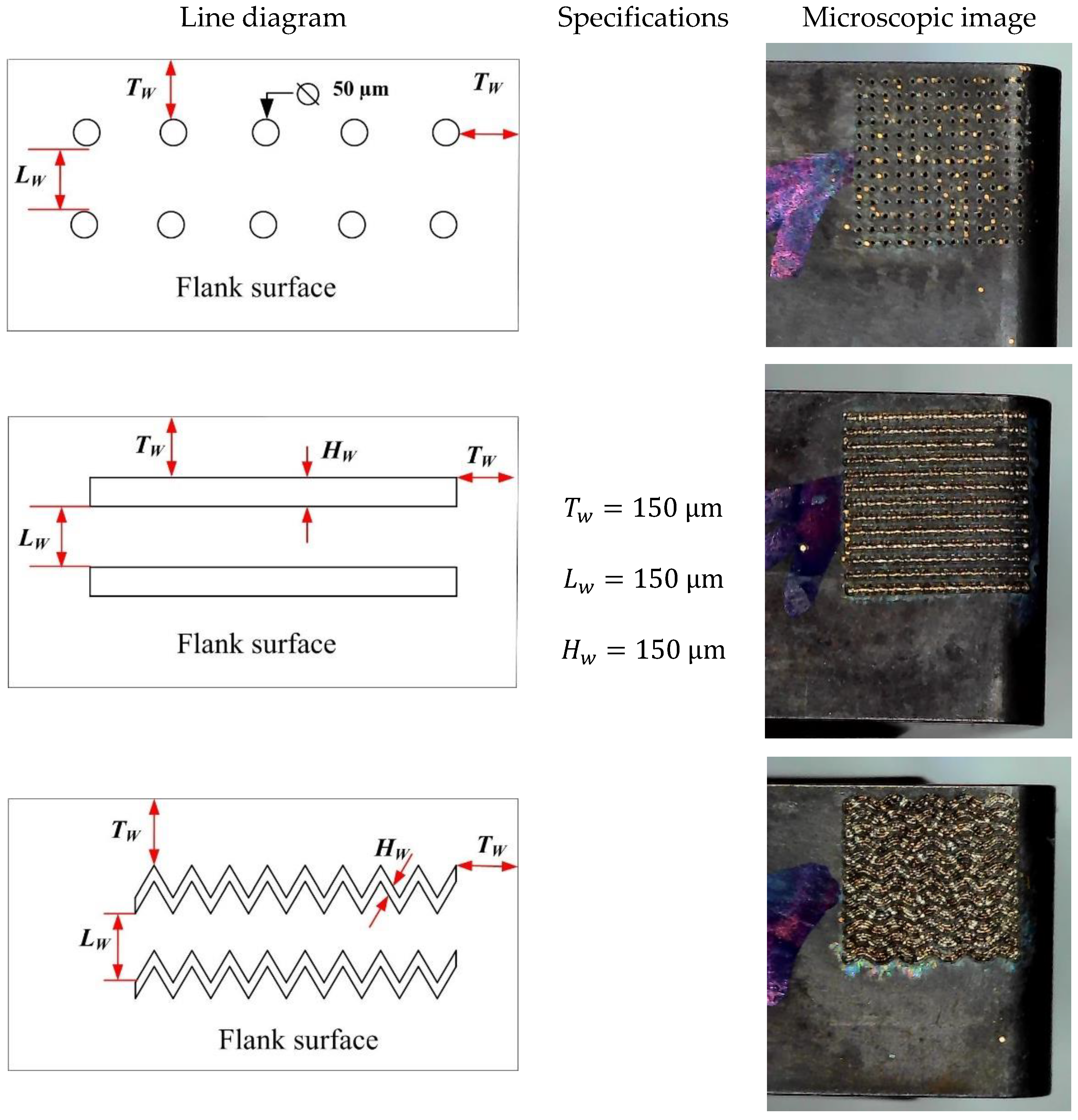
3.1. Experimentation and Measurements

The turning experiments were performed on a Computer Numerical Control (CNC) Ace Micromatic Super Jobber 500 lathe machine, equipped with a spindle motor rated at 7.5 kW. The workpiece material selected was super duplex stainless steel (grade 2507), chosen for its exceptional mechanical strength and superior corrosion resistance. TiAlN-coated (PVD) carbide inserts of grade CNMG 120408 45 DP5010, mounted on an ISO-standard MCLNL 2525 M12 tool holder, were used as cutting tools. To improve machining performance, the flank faces of the inserts were textured with three distinct geometric patterns, namely, groove/channel, dimple, and wave, encompassing both discrete and continuous configurations. Textures were fabricated using an Nd:YAG laser system integrated with a femtosecond laser Meera Micro laser machine tool. The laser parameters were carefully controlled during the texturing process. A wavelength of 1064 nm, a pulse frequency of 3 kHz, a laser power of 3 W, and a scanning speed of 100 mm/s were employed to generate consistent and reproducible texture patterns on the tool surfaces.

All the textured tools were applied to a 2.5 mm $\times$ 2.5 mm square area of the flank surface while maintaining a 150 μm clearance near the nose radius.

For all texture types, a uniform pitch (distance between two consecutive textures) of 150 μm was maintained between consecutive textures. The diameter of the dimples and the width of the grooves and waves were consistently maintained at 50 μm, with a corresponding depth of 50 μm for each texture. The specifications, line diagram, and microscopic images illustrating the geometries of the textured patterns are presented in Figure 4.

A fresh insert was used for each experimental run. Taguchi L₂₇ fractional orthogonal arrays were used to design the experiments, systematically varying the cutting speed (75–100–125 m/min), feed rate (0.06–0.12–0.18 mm/rev), and depth of cut (0.4–0.8–1.2 mm) to assess their influence on surface quality.

Surface roughness was quantified using the parameter mean roughness depth (Rz). Rz is defined as the average of the greatest peak-to-valley heights measured across five sampling lengths within the evaluation length. It quantifies the mean value of the maximum profile height differences, calculated relative to the mean line, and provides an indication of the surface’s vertical roughness characteristics [24].

Rz was selected as the primary response variable due to its high sensitivity to extreme surface deviations, which are critical in evaluating functional performance. By averaging the peak-to-valley distances across multiple sampling lengths, Rz delivers a robust metric for characterizing the true extremities of surface profiles. This makes it particularly advantageous for applications where critical tolerances and surface integrity are paramount. Among various roughness forms, Rz offers a more detailed representation of noticeable surface irregularities captures the maximum peak-to-valley distances, thereby offering greater sensitivity to isolated defects that may significantly influence wear resistance, sealing effectiveness, and fatigue performance. The accurate assessment of Rz is critical for evaluating the effectiveness and precision of machining operations. To ensure accuracy in measurement, a rigorous and standardized methodology was implemented. Following each experimental trial, three Rz measurements were systematically recorded at uniform angular intervals using the Mitutoyo portable Surface Roughness Tester-SJ210, in strict accordance with the ISO 1997 standard [25]. The sampling length was 0.8 mm at 4 mm evaluation length. The measurement direction was perpendicular to the machining direction to accurately capture the surface profile and minimize directional bias.

Table 2. Summary of experiment combinations and corresponding mean roughness depth (Rz) values.

Exp No	Texture Type	vc (m/min)	fr (mm/rev)	dc (mm)	Rz1 (μm)	Rz2 (μm)	Rz3 (μm)	Rz_avg (μm)
1	Dimple	75	0.18	1.2	11.987	8.942	10.104	10.344
2	Dimple	75	0.12	0.8	5.764	6.374	5.460	5.866
3	Dimple	75	0.06	0.4	4.771	4.978	4.538	4.762
4	Dimple	100	0.12	1.2	8.033	10.801	10.523	9.786
5	Dimple	100	0.06	0.8	5.819	6.288	5.353	5.820
6	Dimple	100	0.18	0.4	10.292	8.818	8.212	9.107
7	Dimple	125	0.06	1.2	5.172	5.909	4.671	5.251
8	Dimple	125	0.18	0.8	6.826	6.440	6.781	6.682
9	Dimple	125	0.12	0.4	5.082	5.832	5.500	5.471
1	Groove	75	0.18	1.2	9.255	9.608	9.072	9.312
2	Groove	75	0.12	0.8	6.511	6.331	7.593	6.812
3	Groove	75	0.06	0.4	2.398	2.435	2.402	2.412
4	Groove	100	0.12	1.2	9.843	9.459	9.326	9.543
5	Groove	100	0.06	0.8	4.437	3.839	4.961	4.412
6	Groove	100	0.18	0.4	11.109	7.094	6.401	8.201
7	Groove	125	0.06	1.2	11.536	11.818	10.743	11.366
8	Groove	125	0.18	0.8	4.772	6.512	7.096	6.127
9	Groove	125	0.12	0.4	4.945	5.747	4.674	5.122
1	Wave	75	0.18	1.2	13.817	14.535	14.512	14.288
2	Wave	75	0.12	0.8	7.991	7.598	8.091	7.893
3	Wave	75	0.06	0.4	3.779	3.625	3.290	3.565
4	Wave	100	0.12	1.2	4.720	5.056	5.309	5.028
5	Wave	100	0.06	0.8	5.044	5.062	4.041	4.716
6	Wave	100	0.18	0.4	7.344	6.459	6.363	6.722
7	Wave	125	0.06	1.2	7.697	5.073	11.735	8.168
8	Wave	125	0.18	0.8	7.313	6.529	6.655	6.832
9	Wave	125	0.12	0.4	8.645	9.009	8.395	8.683

provides a summary of the experiments conducted according to L₂₇ and the corresponding Rz values.

3.2. Data Preprocessing for Machine Learning

MATLAB is a robust computational platform widely recognized for its capabilities in data handling, modeling, and the implementation of advanced machine learning (ML) techniques. In this study, MATLAB R2021a was utilized for data preprocessing, augmentation, and model development. Prior to analysis, the dataset underwent a comprehensive inspection to ensure proper loading, verify the presence and structure of all required columns, and confirm the absence of missing or null values.

The dataset comprises four independent variables: cutting speed, feed rate, depth of cut, and texture type. Among these, texture type is a categorical variable further subdivided into three distinct texture geometries, namely, dimple, groove, and wave, each treated as separate input categories. The mean roughness depth (Rz) was selected as the dependent output variable, representing the primary surface quality indicator.

Gaussian Data Augmentation (GDA) has been shown to enhance prediction accuracy and robustness for machine learning models trained on limited datasets [26]. To address potential overfitting associated with the relatively small number of experimental samples, GDA was applied to improve model generalizability [26,27]. In the present study, the original dataset, consisting of 27 experimental runs, was expanded to 81 samples through GDA. Specifically, two augmented data points were generated for each original observation by introducing Gaussian noise to the continuous variables. The standard deviation of the noise was set to 5% of the range of each variable. The categorical variable, texture type, remained unchanged during augmentation to preserve categorical labels across the expanded dataset.

To validate the statistical fidelity of the augmented dataset, a comparative statistical analysis was conducted using the two-sample Kolmogorov–Smirnov (K-S) test to assess the similarity between the original and augmented datasets. The K-S test is a non-parametric method used to compare the distributions of two independent samples without assuming any specific underlying distribution (e.g., normality), making it particularly suitable for real-world data [28].

The test evaluates the maximum vertical distance referred to as the K-S statistic between the empirical cumulative distribution functions (ECDFs) of the two datasets. This metric quantifies the largest discrepancy between the distributions. Under the null hypothesis that both samples originate from the same underlying distribution, the p-value indicates the probability of observing such a difference by chance. The ECDFs of the Rz datasets (n = 27 and n = 81) are shown in Figure 5, visually illustrating the close alignment between the two distributions.

The results yielded a K-S statistic of 0.0741 and a p-value of 0.9998. The small K-S statistic suggests a high degree of similarity between the cumulative distributions of the original and augmented datasets. Furthermore, the p-value is substantially greater than the conventional significance level of 0.05, providing strong statistical evidence in favor of the null hypothesis. Consequently, there is no basis to reject the hypothesis that the two datasets come from the same distribution.

This outcome confirms that the augmented dataset retains the statistical characteristics of the original dataset. Therefore, either dataset can be reliably used for subsequent modeling or analysis. Moreover, it validates that the larger dataset (n = 81) is statistically representative of the smaller dataset (n = 27), reinforcing the effectiveness of the augmentation strategy in preserving the underlying data structure.

Subsequently, the augmented dataset was partitioned into training and testing subsets using an 80:20 split, a commonly adopted approach in machine learning studies [29]. Accordingly, 65 samples (80%) were allocated for training, while 16 samples (20%) were reserved for testing. The careful selection of the test dataset ensured adequate representation across all levels of both continuous and categorical variables, enabling a comprehensive evaluation of the model’s predictive performance.

To ensure balanced contributions from each input feature during model training, data normalization was performed. All continuous input variables were normalized using the standard scaler method, which transforms the data to have zero mean and unit variance. The categorical variable, texture type, was encoded using one-hot encoding to facilitate its integration into the machine learning models. These preprocessing steps were critical for ensuring the reliability and validity of the subsequent analyses.

4. Implementation of Machine Learning Techniques

In the present study, two distinct machine learning techniques, Least-Squares Support Vector Machine (LSSVM) and Multi-Gene Genetic Programming (MGGP), were implemented to develop predictive models for surface roughness (Rz) in machining processes. Both techniques were selected for their ability to capture complex, nonlinear relationships between machining parameters and surface finish quality. Both predictive models were developed and implemented using the MATLAB platform, which provided a flexible environment for algorithm development, training, and evaluation.

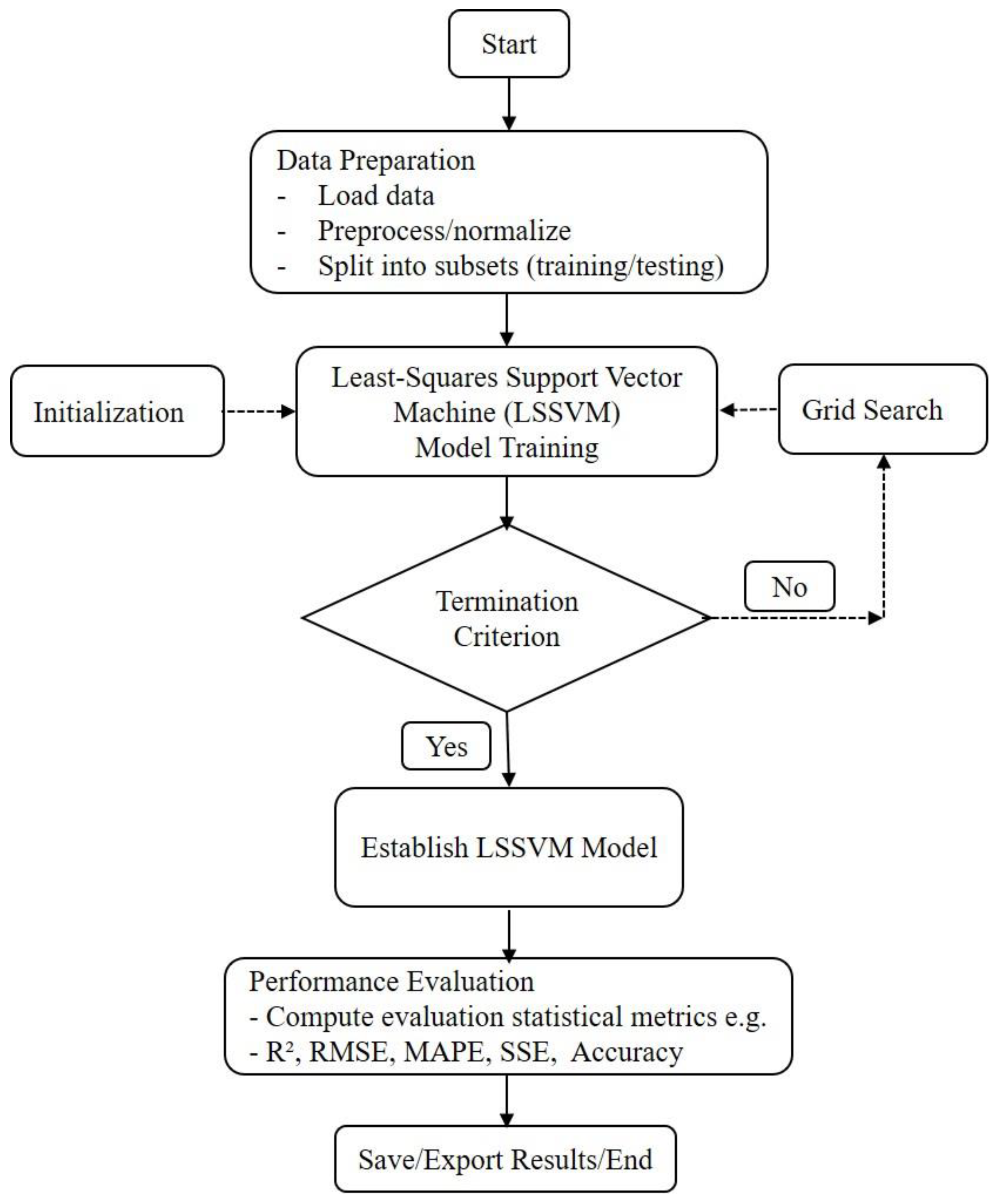
4.1. Least-Squares Support Vector Machine (LSSVM)

The LSSVM model was configured for function estimation, utilizing a radial basis function (RBF) kernel due to its effectiveness in capturing nonlinear relationships. Hyperparameters, namely, the regularization parameter (gam) and the RBF kernel parameter (sig2), were optimized using a grid search strategy in conjunction with leave-one-out cross-validation and mean squared error (MSE) as the performance criterion. After hyperparameter tuning, the model was initialized and trained using the optimized settings. This configuration enabled the LSSVM model to produce a reliable and generalizable mapping from input parameters to the surface roughness output. The detailed summary of the LSSVM model implementation, including key parameters, is shown in

Table 3. LSSVM tuning summary and final hyperparameters.

Category	Metric	Value
Tuning Process	Optimization Method	Grid Search
	Kernel Function	RBF_kernel
	Cost Function	leaveoneoutlssvm
	Grain (log scale optimization)	7
Initial Parameters	Starting gamma	0.93614
	Starting sig2	0.022631
	Cost of Starting Values	3.2322
	Time per Evaluation (sec)	0.015625
	Grid Limits [gamma]	0.9361–2790.6037
	Grid Limits [sig2]	0.022631–3.3588
Final Hyperparameters	gamma	23.1689
	sig2	0.294524

.

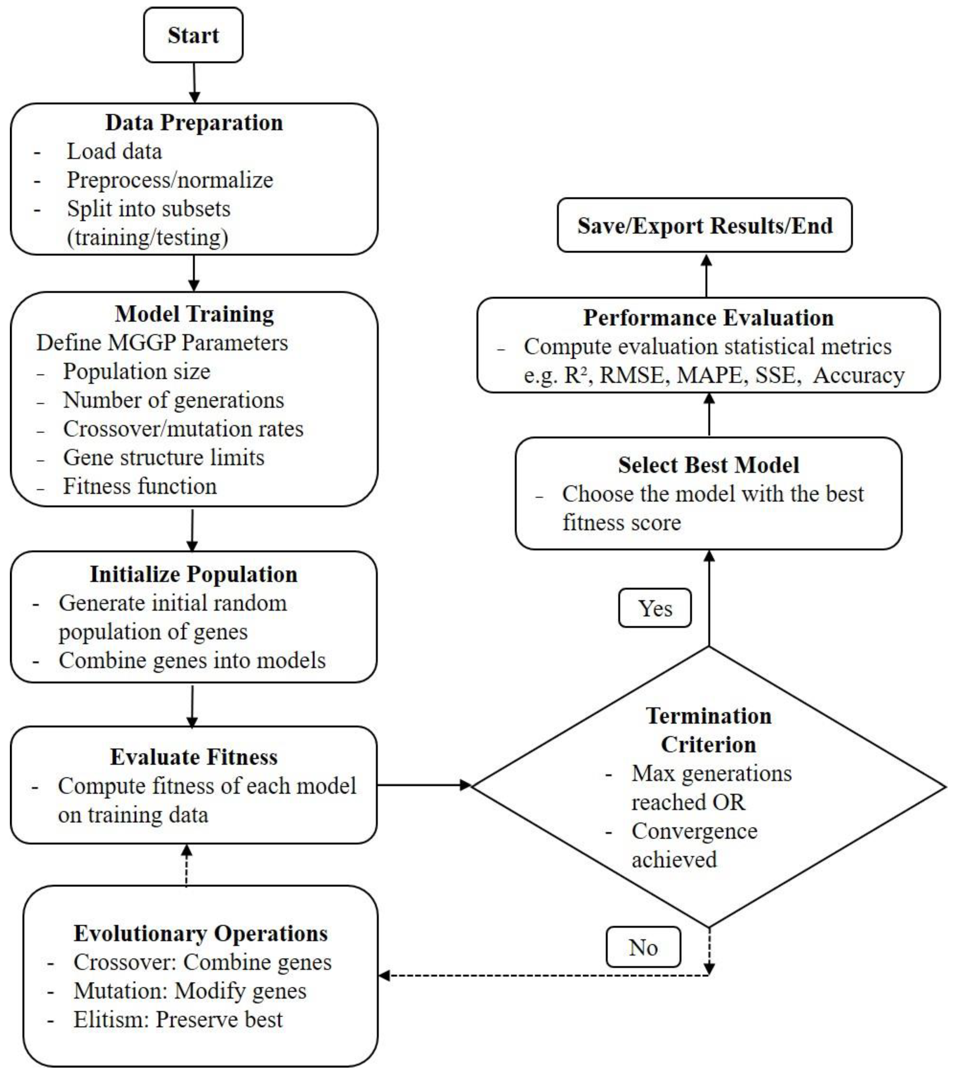
4.2. Multi-Gene Genetic Programming (MGGP)

MGGP was implemented using the GPTIPS 2 framework to perform symbolic regression on surface roughness (Rz) data, simulating a nonlinear process. The population size was set to 100 individuals per generation, and the evolutionary process was constrained by a timeout limit of 10 s per run, across a total of 3 independent runs to ensure reproducibility and robustness. Tournament selection was employed with a tournament size of 6 and a Pareto tournament probability of 0.7, while elitism was applied by retaining the top 70% of individuals in each generation. The fitness evaluation was configured to terminate runs early if a termination criterion was met, with a target fitness value threshold of 0.2. Up to 8 genes were allowed per individual, facilitating the construction of complex symbolic expressions. The set of function nodes used for model construction included basic arithmetic operators and common nonlinear functions: {times, minus, plus, sin, cos, exp, tanh, plog}. These settings collectively enabled the generation of interpretable and high-performing symbolic models for the prediction of Rz in the present work and summarized in

Table 4. MGGP model configuration and run parameters.

Parameter	Setting/Value
Framework	GPTIPS 2
Population size	100 individuals per generation
Evolution runs	3 independent runs
Timeout limit	10 s per run
Selection method	Tournament selection
Tournament size	6
Pareto tournament probability	0.7
Elitism	Top 70% of individuals retained per generation
Early termination criteria	Target fitness value ≤0.2
Maximum number of genes	8 per individual
Function node set	times, minus, plus, sin, cos, exp, tanh, plog

.

The mathematical expression generated by the MGGP model is presented below in Equation (5).

$$\begin{array}{cc}Rz=& 1.09\left({\mathrm{x}}_6-\mathrm{c}\mathrm{o}\mathrm{s}\left({\mathrm{x}}_3\right)\right)+1.77\mathrm{t}\mathrm{a}\mathrm{n}\mathrm{h}\left({\mathrm{x}}_1{\mathrm{x}}_6\left({\mathrm{x}}_4+{\mathrm{x}}_5\right)\right)-0.87\mathrm{l}\mathrm{o}\mathrm{g}\left(\mathrm{a}\mathrm{b}\mathrm{s}\left({\mathrm{x}}_1,{\mathrm{x}}_4\right)\right)-3.3\mathrm{s}\mathrm{i}\mathrm{n}\left(\mathrm{l}\mathrm{o}\mathrm{g}\left(\mathrm{a}\mathrm{b}\mathrm{s}\left({\mathrm{x}}_1{\mathrm{x}}_4\right)\right)\right)\hfill \\ \hfill & -2.57\mathrm{c}\mathrm{o}\mathrm{s}\left(\mathrm{s}\mathrm{i}\mathrm{n}\left({\mathrm{x}}_5\right)\mathrm{s}\mathrm{i}\mathrm{n}\left({\mathrm{x}}_6\right)\right)+2.04\mathrm{t}\mathrm{a}\mathrm{n}\mathrm{h}\left({\mathrm{x}}_2{\mathrm{x}}_8\mathrm{c}\mathrm{o}\mathrm{s}\left({\mathrm{x}}_5\right)\right)-3.66\mathrm{s}\mathrm{i}\mathrm{n}\left(\mathrm{c}\mathrm{o}\mathrm{s}\left({\mathrm{x}}_4-{\mathrm{x}}_6\right)\right)\hfill \\ \hfill & +1.56{\mathrm{x}}_2{\mathrm{x}}_6{(\mathrm{x}}_4-{\mathrm{x}}_5)+11.1\hfill \end{array}$$

(5)

where ${\mathrm{x}}_1, {\mathrm{x}}_{2,} {{\mathrm{x}}_3,{\mathrm{x}}_4,\mathrm{x}}_{5,} {\mathrm{x}}_6$ represent the dimple texture, groove texture, wave texture, $v_c$, $f_r$, and $d_c$ respectively. The final expression consisted of 8 genes with a maximum tree depth of 4, offering a balance between complexity and interpretability. The resulting model for surface roughness (Rz) includes combinations of arithmetic, trigonometric, logarithmic, and hyperbolic functions such as $tanh(x₁x₆(x₄+x₅\left)\right)$ and $cos\left(sin\right(x₅\left)sin\right(x₆\left)\right)$, indicating complex nonlinear interactions between input variables.

Of the modeling approaches considered in this study, MGGP generates explicit analytical expressions that describe the relationship between input variables and the response variable. In contrast, LSSVM functions as a black-box model, wherein the internal mapping from inputs to outputs is not expressed in a closed-form equation.

5. Results and Discussion

5.1. Effect of Machining Parameters on Rz

In the present study, SDSS 2507 was machined in a dry environment using textured inserts, with a primary focus on surface roughness. The surface roughness of machined components is significantly influenced by machining parameters. To systematically assess their effects, the Taguchi method has emerged as a widely adopted technique, providing a robust and efficient framework for identifying key factors and analyzing their impact on the response variable [30].

A Taguchi-based signal-to-noise (S/N) ratio analysis was employed to evaluate the influence of machining parameters, namely, cutting speed, feed rate, cutting depth, and tool texture type, on the surface roughness of the machined components. The S/N ratio quantifies the consistency of a response relative to the target value, with higher ratios signifying reduced variability and enhanced performance. The selection of the appropriate S/N ratio formulation depends on the nature of the response being examined and the experimental objectives. Common formulations include “larger is better,” which prioritizes maximization, “nominal is best,” which emphasizes precision around a target value, and “smaller is better,” which aims to minimize undesirable deviations [14].

The main effect plots for the S/N ratios were generated using the “smaller is better” criterion, as lower Rz values are desirable for achieving quality machined components. The results are summarized in

Table 5. Response table for signal-to-noise ratios.

Level	Texture Type	Cutting Speed (vc)	Feed Rate (fr)	Depth of Cut (dc)
1	−16.58	−16.11	−14.19	−14.89
2	−16.17	−16.57	−16.79	−15.62
3	−16.65	−16.71	−18.41	−18.89
Delta	0.48	0.6	4.23	4
Rank	4	3	1	2

and illustrated in Figure 6. These visual representations facilitate the identification of trends and the assessment of individual parameter influences, thereby enabling improved control over surface quality during machining operations.

As presented in Table 2, the minimum Rz value of 2.412 µm was achieved using the groove-textured tool at a cutting speed of 75 m/min, a feed rate of 0.06 mm/rev, and a depth of cut of 0.4 mm. Conversely, the maximum Rz value of 14.288 µm was observed with the wave-textured tool under the same cutting speed but at a higher feed rate of 0.18 mm/rev and a greater depth of cut of 1.2 mm. Figure 6 depicts the influence of machining parameters on surface roughness through the main effects plot of the S/N ratios, offering a visual interpretation of each factor’s relative contribution.

The delta value represents the effect of each input factor on the response by calculating the difference between the maximum and minimum signal-to-noise (S/N) ratios across its levels [31]. A larger delta value indicates a greater influence of the corresponding factor on the output. As presented in Table 5, the delta values indicate that feed rate is the most influential parameter affecting surface roughness, followed by depth of cut, cutting speed, and tool texture type. This finding is consistent with established machining theory, where feed rate is widely recognized as a critical determinant of surface finish [32]. Furthermore, the main effect plots illustrated in Figure 6 reveal that an increase in feed rate leads to a notable reduction in the S/N ratio, indicating a deterioration in surface quality, i.e., Rz, in line with the literature [12,33]. This trend aligns with the theoretical relationship between surface roughness and feed rate, wherein surface roughness increases proportionally with feed rate. Such consistency between experimental results and theoretical expectations reinforces the validity of the observed influence of feed rate on surface finish.

Furthermore, as shown in Figure 6, increasing cutting parameter levels leads to a decline in signal-to-noise (S/N) ratios, reflecting a deterioration in surface quality. This trend is attributed to intensified mechanical and thermal stresses, which exacerbate wear mechanisms and negatively impact the machined surface. Additionally, cutting speed, feed rate, and depth of cut consistently reduce S/N ratios, underscoring their adverse influence on surface roughness at elevated levels.

5.2. Model Evaluation

Following the development of the machine learning models, a comprehensive evaluation of their predictive performance was conducted by analyzing the relationship between the actual and predicted values of Rz for both the training and testing datasets. The results of this analysis are presented in Figure 7 and Figure 8, which correspond to the training and testing datasets, respectively.

As depicted in Figure 7, the predicted Rz values demonstrate strong alignment with the actual values across both models: Least-Squares Support Vector Machine (LSSVM) and Multi-Gene Genetic Programming (MGGP). The close correspondence between the predicted and actual values underscores the ability of each model to effectively capture the underlying nonlinear relationships within the training data. This outcome highlights the high learning accuracy and robustness of the models during the training phase.

In the case of the testing dataset, as shown in Figure 8, both models exhibit admirable generalization capabilities. While minor discrepancies are observed in certain instances, they were consistent in each case and more prominently deviated in the MGGP model. Overall trends remain consistent with those observed during the training phase. These findings confirm that the models not only achieve an excellent fit on the training data but also maintain reliable performance when applied to unseen data. Such results validate the practical applicability of the developed models for predicting surface roughness in machining processes, thereby emphasizing their potential utility in real-world industrial settings.

5.3. Comparative Evaluation of Machine Learning Models’ Performances

In this study, the performance of the models was rigorously evaluated on both the training and testing datasets to ensure the reliability and generalization capacity of the considered models. The evaluation process involved systematically comparing estimated values with actual observations, thereby assessing each model’s ability to capture underlying patterns without overfitting. This dual-phase validation approach facilitated an assessment of how effectively the model learned from the training data and its capacity to generalize to unseen data. To quantitatively evaluate the predictive performance of the developed models, the evaluation metrics employed in this study encompass a comprehensive set of statistical measures, including the coefficient of determination (R²), root mean squared error (RMSE), mean absolute error (MAE), mean absolute percentage error (MAPE), mean squared error (MSE), sum of squared errors (SSE), and accuracy, as shown in Equations (6)–(11) [18].

$$R^2=1-\left({\displaystyle \frac{\sum {\left(Aᵢ-Pᵢ\right)}^2}{\sum {\left(Aᵢ-\overline{A}\right)}^2}}\right)$$

(6)

where $A\mathrm{ᵢ}$ is the actual value, $P\mathrm{ᵢ}$ is the predicted value, and $\overline{A}$ is the mean of the actual values. RMSE represents the square root of the average squared differences between actual and predicted values:

$$RMSE=\sqrt{{\displaystyle \frac{{\sum }_{i=1}^n{\left(A\mathrm{ᵢ}-P\mathrm{ᵢ}\right)}^2}{n}}}$$

(7)

MAE is the average of the absolute differences:

$$MAE={\displaystyle \frac{{\sum }_{i=1}^n|A\mathrm{ᵢ}-P\mathrm{ᵢ}|}{n}}$$

(8)

MAPE evaluates the mean absolute percentage difference between predicted and actual values:

$$MAPE={\displaystyle \frac{100}{n}}\%\times {\sum }_{i=1}^n\left|{\displaystyle \frac{A\mathrm{ᵢ}-P\mathrm{ᵢ}}{A\mathrm{ᵢ}}}\right|$$

(9)

SSE calculates the total squared deviation:

$$SSE={\sum }_{i=1}^n{\left(A\mathrm{ᵢ}-P\mathrm{ᵢ}\right)}^2$$

(10)

Finally, accuracy assesses how close predictions are in absolute terms:

$$Accuracy=1-\left[{\displaystyle \frac{1}{n}}{\sum }_{i=1}^n{\displaystyle \frac{\left|A\mathrm{ᵢ}-P\mathrm{ᵢ}\right|}{\left|A\mathrm{ᵢ}\right|}}\right]$$

(11)

Here, $n$ is the number of observations (samples). These performance metrics collectively provide a robust evaluation of each model’s predictive capability and generalization performance. The calculated values of R², RSME, MAE, MAPE, SSE, and accuracy for both models on the training dataset are summarized in

Table 6. Statistical performance metrics of ML models on training dataset.

	LSSVM	MGGP
R2	0.9959 *	0.8480
RMSE	0.1528 *	0.9333
MAE	0.1247 *	0.6772
MAPE	2.0089	0.1096 *
SSE	1.5173 *	56.6200
Accuracy	0.9814 *	0.8904

* Best-performing value for each metric.

, providing a basis for detailed comparative analysis of their learning performance and robustness.

The coefficient of determination (R²) was found to exceed 84% for both models, with particularly strong values for LSSVM, surpassing 99%. These results indicate that the models possess strong explanatory power and accurately capture the variance in the training dataset. Furthermore, the RMSE values for all models were below 1, with the LSSVM model achieving an exceptionally low RMSE of 0.1528, reflecting minimal deviation between the predicted and actual values. Similarly, the MAE and MAPE values were also notably low, further confirming the high predictive precision of the models. The sum of squared errors (SSE) was minimal for the LSSVM model, whereas the MGGP model exhibited a relatively higher SSE, though it remained within an acceptable range. In terms of prediction accuracy, both models performed well, averaging around 90%, with LSSVM achieving outstanding accuracies of 98.14%. Overall, the statistical metrics demonstrate that the developed models effectively learned from the training dataset and achieved high prediction accuracy with minimal error, validating their robustness and suitability for surface roughness prediction. Figure 9 summarizes the comparative performance of the models on the training dataset based on key statistical metrics.

In Figure 9, the bar chart highlights the best-performing values for each statistical metric, marked with a green fill. This indicates that LSSVM outperforms MGGP by achieving the highest R² and accuracy values, along with the lowest error metrics. The only exception is MAPE, where LSSVM shows a slightly higher value compared to MGGP.

The statistical metrics calculated on the testing dataset are summarized in

Table 7. Statistical performance metrics of ML models on testing dataset.

	LSSVM	MGGP
R2	0.9391 *	0.6444
RMSE	0.6730 *	1.6265
MAE	0.4817 *	1.3754
MAPE	6.6363 *	0.1850
SSE	7.2478 *	42.3300
Accuracy	0.9436 *	0.8150

* Best-performing value for each metric.

, providing an overview of the models’ performance on unseen data (testing dataset).

A general observation from the calculated statistical metrics as shown in Table 7 reveals that both models performed well on the testing dataset. However, the impact of unseen data is evident, with slight deterioration in the metric values. Despite this, both models successfully captured the nonlinear behavior of the input parameters, demonstrating robustness in predicting on the unseen testing dataset. The R² values for the LSSVM model were above 93%, whereas the MGGP model achieved an R² of 64.44%. The RMSE values remained below 1 for the LSSVM model, while the MGGP model recorded an RMSE of 1.6265. Both MAE and MAPE values were very low, remaining below 1 for the LSSVM model, while MGGP recorded a value of 1.3754. SSE values were also low for both models, with MGGP showing slightly higher values, though still within an acceptable range.

The prediction accuracy for both models was notably high, with LSSVM achieving accuracies around 95%, while MGGP achieved 82%. These results highlight the strong predictive capabilities of both LSSVM and MGGP models, particularly in handling unseen data. Figure 10 provides a comparative overview of the models’ performance on the testing dataset, as evaluated through key statistical metrics.

In Figure 10, the bar chart visually emphasizes the best-performing values for each statistical metric, indicated by an orange fill. This graphical representation underscores the LSSVM model as the most effective in capturing the underlying patterns within the testing dataset. Consistent with its performance on the training dataset, LSSVM outperformed the MGGP model, further highlighting its superior predictive capabilities on unseen data.

To assess the accuracy and reliability of the MGGP and LSSVM models in predicting surface roughness (Rz), statistical hypothesis testing was performed. A paired two-sample t-test was used to evaluate whether there is a significant difference in the means of actual and predicted values, while an F-test compared the variances of the two datasets. These tests provide insight into whether the models produce unbiased predictions and replicate the variability observed in the experimental measurements [18]. The results of the t-tests and F-tests are summarized in

Table 8. Summary of t-test and F-test results.

Model	t-Test		F-Test		Pearson Correlation (r)
	t-Statistic	p-Value	F-Statistic	p-Value
MGGP	−0.425	0.672	1.08	0.367	0.90
LSSVM	0.754	0.453	1.12	0.307	0.99

.

The paired t-tests for both models indicated no significant difference in the mean values of actual and predicted surface roughness, demonstrating that both models produce unbiased estimations. The F-tests similarly showed no significant difference in variances, suggesting that the models capture the variability of the experimental data well. The higher Pearson correlation of the LSSVM model (r = 0.99) compared to MGGP (r = 0.90) indicates a stronger linear relationship with the actual measurements. Overall, both models exhibit strong predictive performance, with LSSVM showing slightly higher correlation accuracy.

6. Conclusions

This study developed and validated a machine learning-based framework for accurately predicting surface roughness (Rz) during the dry machining of super duplex stainless steel (SDSS 2507), a material known for its outstanding mechanical strength and corrosion resistance but inherently difficult machinability. The framework leveraged textured cutting tools (dimple, groove, and wave) and systematically analyzed the influence of cutting speed, feed rate, depth of cut, and tool texture on the surface quality of SDSS 2507. The following important conclusions can be drawn:

• Feed rate was found to be the most influential parameter affected mean roughness depth.
• To obtain better surface quality, the machining of SDSS 2507 at lower values of machining parameters is recommended.
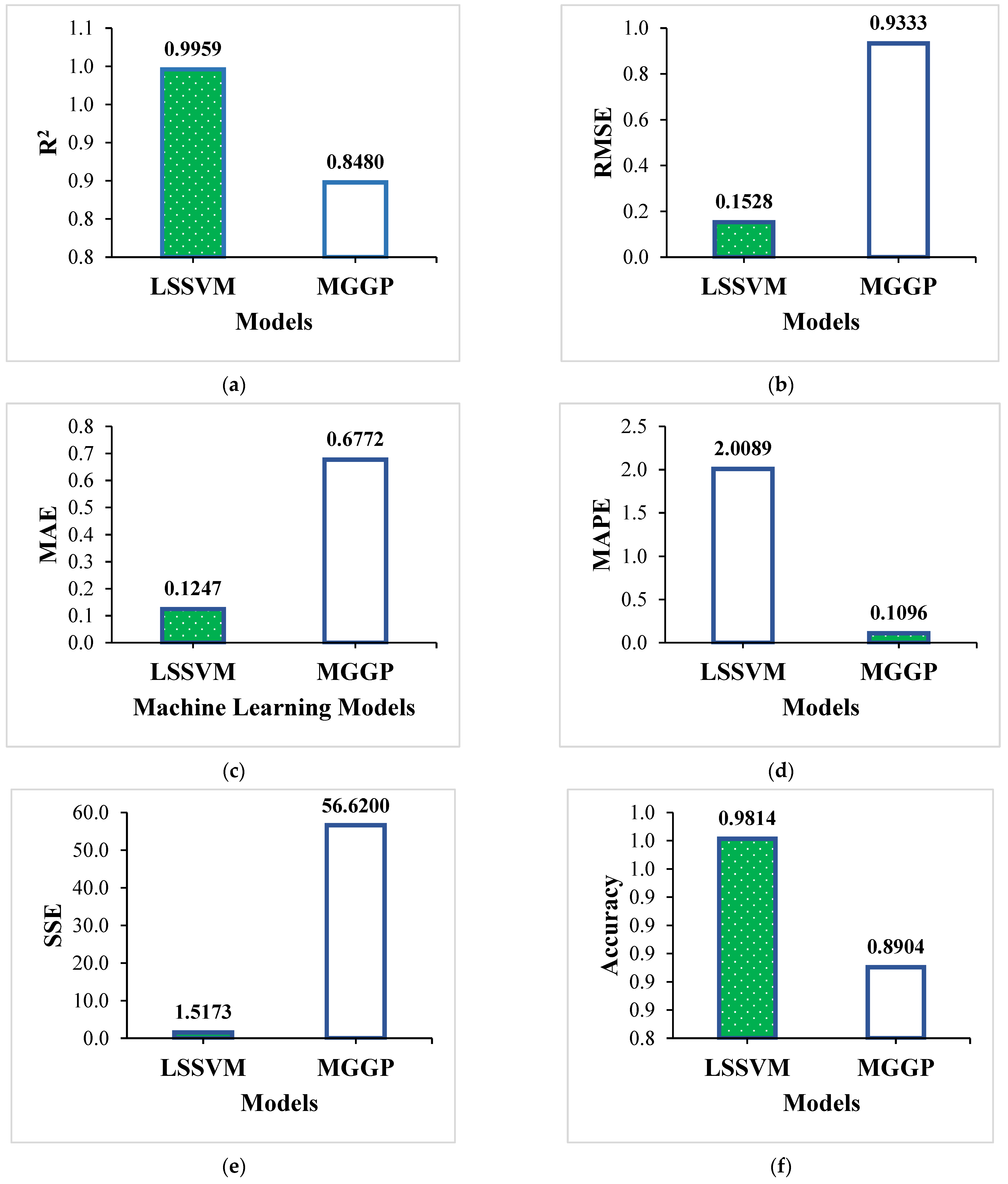
• The Least-Squares Support Vector Machine (LSSVM) model demonstrated superior predictive performance, achieving an R² of 0.9959 and 98.14% accuracy on the training dataset, and maintaining strong generalization on unseen data with a testing R² of 0.9391 and an accuracy of 94.36%, outperforming the Multi-Gene Genetic Programming (MGGP) model.
• The MGGP model also showed reasonable performance with a training R² of 0.8480 and a testing R² of 0.6444, though it was less effective than LSSVM in minimizing prediction errors across all evaluated metrics.
• Comprehensive statistical validation using metrics such as RMSE, MAE, MAPE, SSE, and accuracy confirmed the reliability of the LSSVM model for accurate surface roughness prediction.

The findings of this research confirm the strong predictive capability and reliability of the LSSVM model for surface roughness prediction, making it a highly suitable tool for practical applications.

Future research may explore the application of hybrid and ensemble machine learning techniques to further improve predictive accuracy and model robustness. Additionally, leveraging the predictive capabilities of these models by integrating them into process optimization frameworks offers a promising approach for achieving optimal surface roughness and enhancing overall machining efficiency. Future work investigating the influence of texture type on roughness and tool wear and their relationship can help to establish the field further.

References

1. Reffas, O.; Boumediri, H.; Karmi, Y.; Kahaleras, M.S.; Bousba, I.; Aissa, L. Statistical Analysis and Predictive Modeling of Cutting Parameters in EN-GJL-250 Cast Iron Turning: Application of Machine Learning and MOALO Optimization. Int. J. Adv. Manuf. Technol. 2025, 137, 1991–2009. [Google Scholar] [CrossRef]
2. Kumar, S.T.P.; Prasada, H.P.T.; Nagamadhu, M.; Pattar, N.; Kivade, S.B.; Sachinkumar; Ravichandra, K.R.; Hanumanthlal, S. Experimental Investigation on the Performance of Different Cutting Fluids on Cutting Force During Turning of Duplex Stainless Steel-2205 under MQL Technique. Math. Model. Eng. Probl. 2022, 9, 136–143. [Google Scholar] [CrossRef]
3. Khlifi, H.; Abdellaoui, L.; Saï, W.B. Prediction of Cutting Force and Surface Roughness in Turning Using Machine Learning. 2nd International Conference on Innovative Materials, Manufacturing and Advanced Technologies, IMMAT 2022. Mech. Mach. Sci. 2024, 144, 213–222. [Google Scholar]
4. Zhang, Y.; Xu, X. Machine Learning Cutting Force, Surface Roughness, and Tool Life in High Speed Turning Processes. Manuf. Lett. 2021, 29, 84–89. [Google Scholar] [CrossRef]
5. Abellán-Nebot, J.V.; Vila Pastor, C.; Siller, H.R. A Review of the Factors Influencing Surface Roughness in Machining and Their Impact on Sustainability. Sustainability 2024, 16, 1917. [Google Scholar] [CrossRef]
6. Dubey, V.; Sharma, A.K.; Pimenov, D.Y. Prediction of Surface Roughness Using Machine Learning Approach in MQL Turning of AISI 304 Steel by Varying Nanoparticle Size in the Cutting Fluid. Lubricants 2022, 10, 81. [Google Scholar] [CrossRef]
7. Jacob, J.; Meurer, M.; Bergs, T. Surface Roughness Prediction in Hard Turning (Finishing) of 16MnCr5 Using a Model Ensemble Approach. Procedia CIRP 2024, 126, 504–507. [Google Scholar] [CrossRef]
8. Yeganefar, A.; Niknam, S.A.; Asadi, R. The Use of Support Vector Machine, Neural Network, and Regression Analysis to Predict and Optimize Surface Roughness and Cutting Forces in Milling. Int. J. Adv. Manuf. Technol. 2019, 105, 951–965. [Google Scholar] [CrossRef]
9. Pimenov, D.Y.; Bustillo, A.; Mikolajczyk, T. Artificial Intelligence for Automatic Prediction of Required Surface Roughness by Monitoring Wear on Face Mill Teeth. J. Intell. Manuf. 2018, 29, 1045–1061. [Google Scholar] [CrossRef]
10. Gupta, M.K.; Mia, M.; Pruncu, C.I.; Khan, A.M.; Rahman, M.A.; Jamil, M.; Sharma, V.S. Modeling and Performance Evaluation of Al2O3, MoS2 and Graphite Nanoparticle-Assisted MQL in Turning Titanium Alloy: An Intelligent Approach. J. Braz. Soc. Mech. Sci. Eng. 2020, 42, 207. [Google Scholar] [CrossRef]
11. Balonji, S.; Tartibu, L.K.; Okokpujie, I.P. Prediction Analysis of Surface Roughness of Aluminum Al6061 in End Milling CNC Machine Using Soft Computing Techniques. Appl. Sci. 2023, 13, 4147. [Google Scholar] [CrossRef]
12. Kosarac, A.; Tabakovic, S.; Mladjenovic, C.; Zeljkovic, M.; Orasanin, G. Next-Gen Manufacturing: Machine Learning for Surface Roughness Prediction in Ti-6Al-4V Biocompatible Alloy Machining. J. Manuf. Mater. Process. 2023, 7, 202. [Google Scholar] [CrossRef]
13. Dewangan, A.; Neigapula, V.S.N.; Soni, D.L.; Vaidya, S. Estimation of Surface Quality for Turning Operations Using Machine Learning Approach. Tribol. Mater. Surf. Interfaces 2024, 18, 228–242. [Google Scholar] [CrossRef]
14. Adizue, U.L.; Takács, M. Exploring the Correlation between Design of Experiments and Machine Learning Prediction Accuracy in Ultra-Precision Hard Turning of AISI D2 with CBN Insert: A Comparative Study of Taguchi and Full Factorial Designs. Int. J. Adv. Manuf. Technol. 2025, 137, 2061–2090. [Google Scholar] [CrossRef]
15. Abbas, A.T.; Sharma, N.; Alqosaibi, K.F.; Abbas, M.A.; Sharma, R.C.; Elkaseer, A. Investigation of Surface Quality and Productivity in Precision Hard Turning of AISI 4340 Steel Using Integrated Approach of ML-MOORA-PSO. Processes 2025, 13, 1156. [Google Scholar] [CrossRef]
16. May Tzuc, O.; Hernández-Pérez, I.; Macias-Melo, E.V.; Bassam, A.; Xamán, J.; Cruz, B. Multi-Gene Genetic Programming for Predicting the Heat Gain of Flat Naturally Ventilated Roof Using Data from Outdoor Environmental Monitoring. Measurement 2019, 138, 106–117. [Google Scholar] [CrossRef]
17. Garg, A.; Lam, J.S.L. Improving Environmental Sustainability by Formulation of Generalized Power Consumption Models Using an Ensemble Based Multi-Gene Genetic Programming Approach. J. Clean. Prod. 2015, 102, 246–263. [Google Scholar] [CrossRef]
18. Pawanr, S.; Garg, G.K.; Routroy, S. Prediction of Energy Efficiency, Power Factor and Associated Carbon Emissions of Machine Tools Using Soft Computing Techniques. Int. J. Interact. Des. Manuf. 2023, 17, 1165–1183. [Google Scholar] [CrossRef]
19. Xu, C.; Yao, S.; Wang, G.; Wang, Y.; Xu, J. A Prediction Model of Drilling Force in CFRP Internal Chip Removal Hole Drilling Based on Support Vector Regression. Int. J. Adv. Manuf. Technol. 2021, 117, 1505–1516. [Google Scholar] [CrossRef]
20. Wang, T.; Noori, M.; Altabey, W.A.; Wu, Z.; Ghiasi, R.; Kuok, S.C.; Silik, A.; Farhan, N.S.D.; Sarhosis, V.; Farsangi, E.N. From Model-Driven to Data-Driven: A Review of Hysteresis Modeling in Structural and Mechanical Systems. Mech. Syst. Signal Process. 2023, 204, 110785. [Google Scholar] [CrossRef]
21. Lin, Y.; Li, L.; Yang, S.; Chen, X.; Li, X.; Zhu, Z. Performance Prediction and Optimization of Hydrogenation Feed Pump Based on Particle Swarm Optimization–Least Squares Support Vector Regression Surrogate Model. Eng. Appl. Comput. Fluid Mech. 2024, 18, 2315985. [Google Scholar] [CrossRef]
22. Niazkar, M. Multigene Genetic Programming and Its Various Applications; Elsevier Inc.: Amsterdam, The Netherlands, 2022; ISBN 9780128212851. [Google Scholar]
23. Bardhan, A. Probabilistic Assessment of Heavy-Haul Railway Track Using Multi-Gene Genetic Programming. Appl. Math. Model. 2024, 125, 687–720. [Google Scholar] [CrossRef]
24. Chaubey, S.K.; Gupta, K.; Madić, M. An Investigation on Mean Roughness Depth and Material Erosion Speed During Manufacturing of Stainless-Steel Miniature Ratchet Gears By Wire-Edm. Facta Univ. Ser. Mech. Eng. 2023, 21, 239–258. [Google Scholar] [CrossRef]
25. ISO 4287; Geometrical Product Specifications (GPS)–Surface Texture: Profile Method–Terms, Definitions and Surface Texture Parameters. International Organization for Standardization: Geneva, Switzerland, 1997.
26. Balasuadhakar, A.; Thirumalai Kumaran, S.; Uthayakumar, M. Machine Learning Prediction of Surface Roughness in Sustainable Machining of AISI H11 Tool Steel. Smart Mater. Manuf. 2025, 3, 100075. [Google Scholar] [CrossRef]
27. Avuçlu, E. A New Data Augmentation Method to Use in Machine Learning Algorithms Using Statistical Measurements. Measurement 2021, 180, 109577. [Google Scholar] [CrossRef]
28. Rai, A.; Ahmad, Z.; Hasan, M.J.; Kim, J.M. A Novel Pipeline Leak Detection Technique Based on Acoustic Emission Features and Two-Sample Kolmogorov–Smirnov Test. Sensors 2021, 21, 8247. [Google Scholar] [CrossRef]
29. Zhang, G.; Eddy Patuwo, B.; Hu, M.Y. Forecasting with Artificial Neural Networks: The State of the Art. Int. J. Forecast. 1998, 14, 35–62. [Google Scholar] [CrossRef]
30. Abbed, K.; Kribes, N.; Yallese, M.A.; Chihaoui, S.; Boutabba, S. Effects of Tool Materials and Cutting Conditions in Turning of Ti-6Al-4V Alloy: Statistical Analysis, Modeling and Optimization Using CoCoSo, MABAC, ARAS and CODAS Methods. Int. J. Adv. Manuf. Technol. 2023, 128, 1535–1557. [Google Scholar] [CrossRef]
31. Rathod, N.J.; Chopra, M.K.; Shelke, S.N.; Chaurasiya, P.K.; Kumar, R.; Saxena, K.K.; Prakash, C. Investigations on Hard Turning Using SS304 Sheet Metal Component Grey Based Taguchi and Regression Methodology. Int. J. Interact. Des. Manuf. 2024, 18, 2653–2664. [Google Scholar] [CrossRef]
32. Bhardwaj, B.; Kumar, R.; Singh, P.K. Surface Roughness (Ra) Prediction Model for Turning of AISI 1019 Steel Using Response Surface Methodology and Box-Cox Transformation. Proc. Inst. Mech. Eng. Part B J. Eng. Manuf. 2014, 228, 223–232. [Google Scholar] [CrossRef]
33. Sun, Z.; Liu, Y.; Geng, D.; Zhang, D.; Ying, E.; Liu, R.; Jiang, X. Cutting Performance and Surface Integrity during Rotary Ultrasonic Elliptical Milling of Cast Ni-Based Superalloy. J. Mater. Res. Technol. 2025, 35, 980–994. [Google Scholar] [CrossRef]
Figure 1. Adopted methodology.
Technologies 13 00243 g001
Figure 2. Outline of the LSSVM model based on [6].
Technologies 13 00243 g002
Figure 3. Outline of the MGGP model.
Technologies 13 00243 g003
Figure 4. The specifications and line diagram of the texture geometries used in the present research.
Technologies 13 00243 g004
Figure 5. ECDFs of Rz data: original vs. augmented.
Technologies 13 00243 g005
Figure 6. Main effect plots for S/N ratios.
Technologies 13 00243 g006
Figure 7. Actual vs. predicted values on the training dataset for (a) LSSVM and (b) MGGP.
Technologies 13 00243 g007
Figure 8. Actual vs. predicted values on the testing dataset for (a) LSSVM and (b) MGGP.
Technologies 13 00243 g008
Figure 9. Comparison of models based on key statistical metrics on training dataset: (a) R2, (b) RMSE, (c) MAE, (d) MAPE, (e) SSE, and (f) accuracy.
Technologies 13 00243 g009
Figure 10. Comparison of models based on key statistical metrics on testing dataset: (a) R2, (b) RMSE, (c) MAE, (d) MAPE, (e) SSE, and (f) accuracy.
Technologies 13 00243 g010