
Application of Machine Learning Methods for Identifying Wave Aberrations from Combined Intensity Patterns Generated Using a Multi-Order Diffractive Spatial Filter

 ,
,  ,
,  and
and 
Abstract
1. Introduction
2. Materials and Methods
2.1. Theoretical Foundations
2.2. Dataset
2.3. CNN Architecture
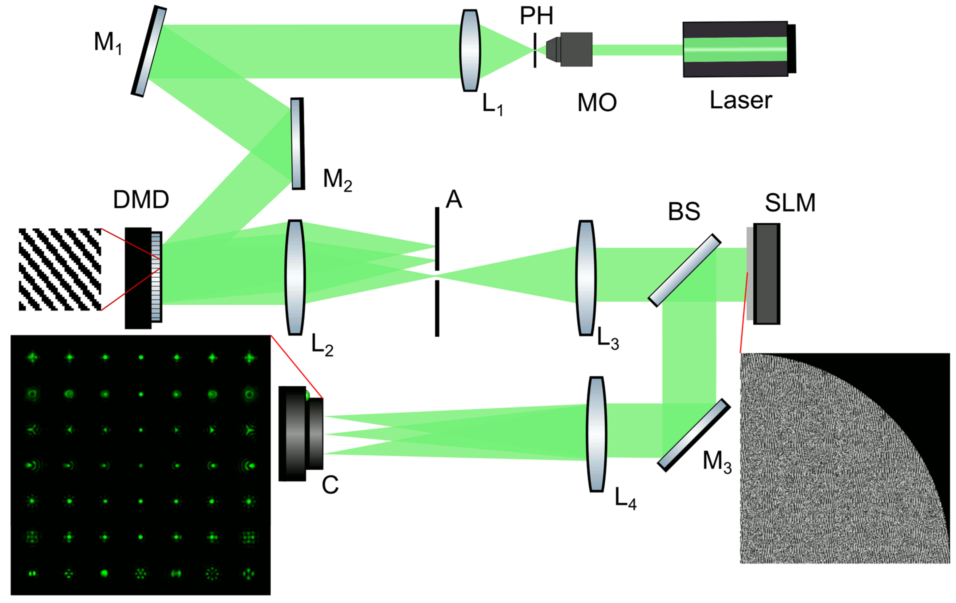
2.4. Optical Scheme
3. Results
3.1. Modeling Dataset
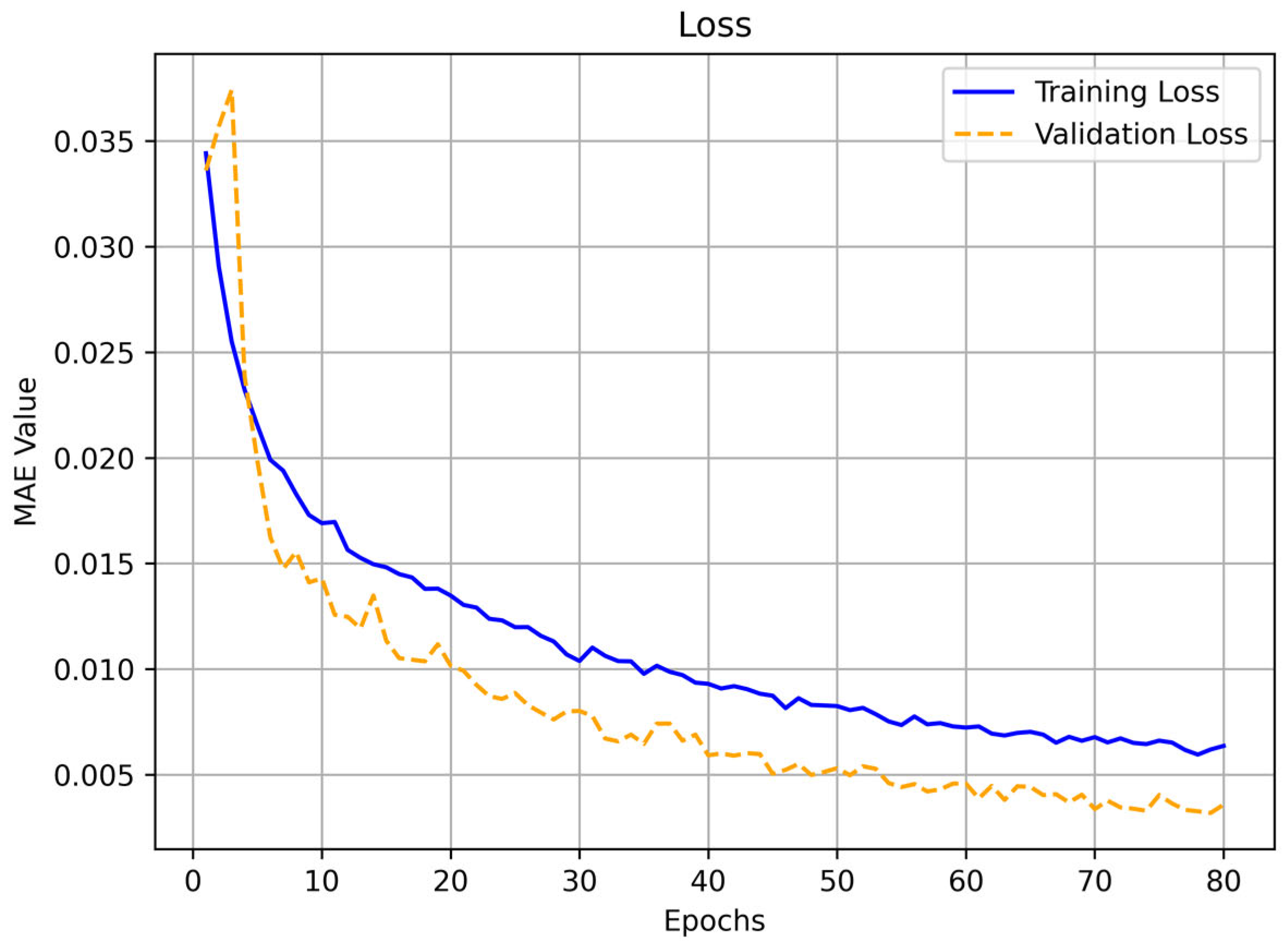
3.2. CNN Training
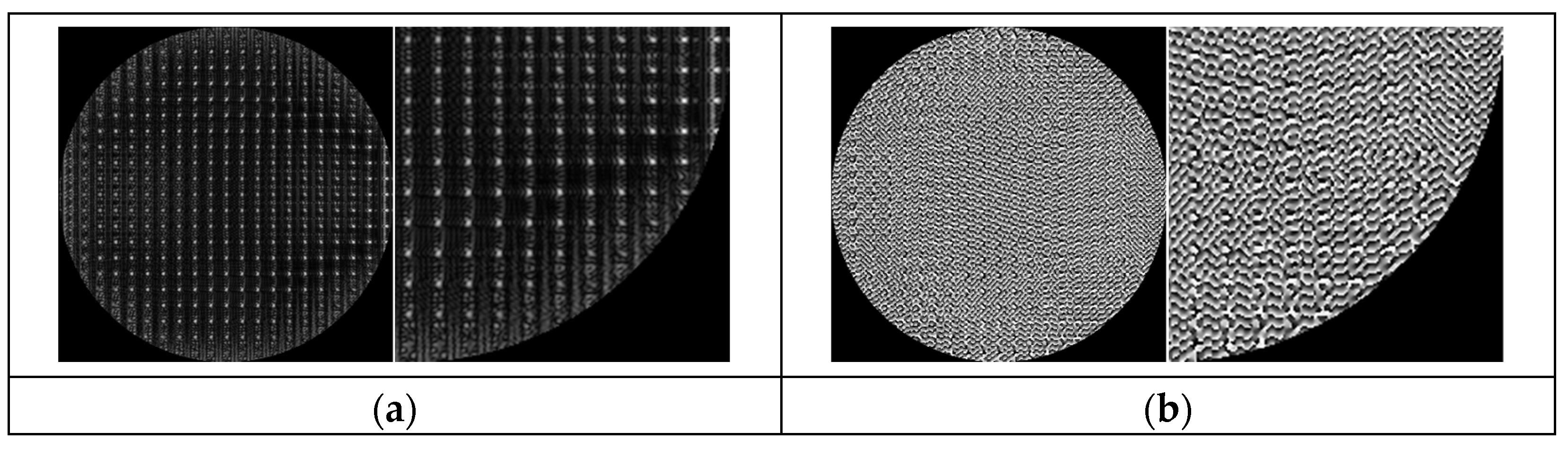
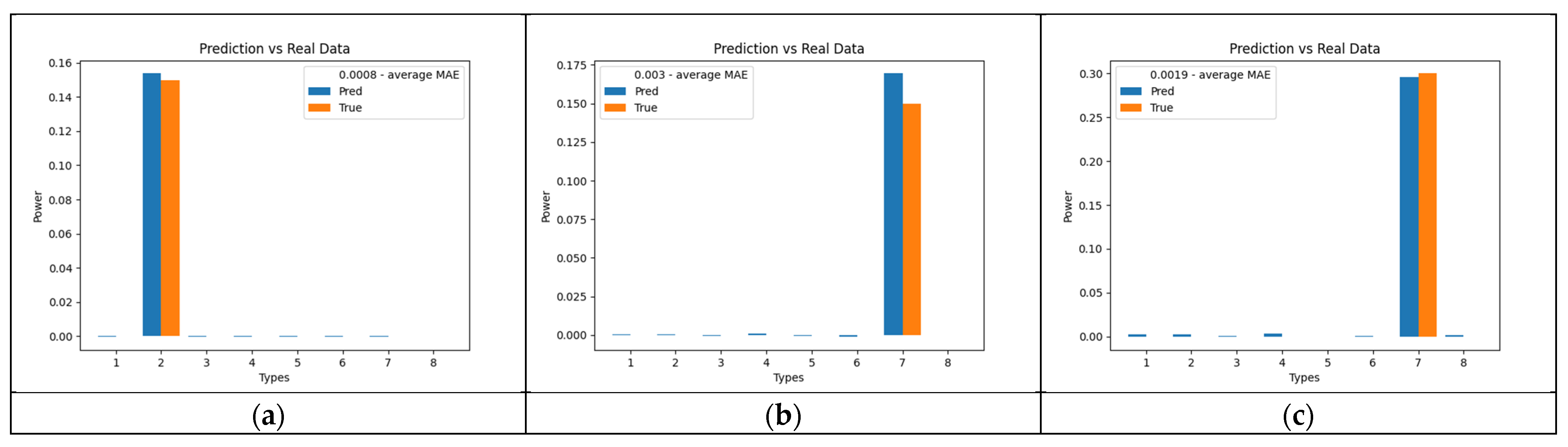
3.3. Experimental Results
4. Discussion
5. Conclusions
Author Contributions
Funding
Institutional Review Board Statement
Informed Consent Statement
Data Availability Statement
Acknowledgments
Conflicts of Interest
References
- El Srouji, L.; Krishnan, A.; Ravichandran, R.; Lee, Y.; On, M.; Xiao, X.; Ben Yoo, S.J. Photonics and optoelectronic neuromorphic computing. APL Photonics 2022, 7, 051101. [Google Scholar] [CrossRef]
- Kazanskiy, N.L.; Butt, M.A.; Khonina, S.N. Optical Computing: Status and Perspectives. Nanomaterials 2022, 12, 2171. [Google Scholar] [CrossRef]
- Liao, K.; Dai, T.; Yan, Q.; Hu, X.; Gong, Q. Integrated Photonic Neural Networks: Opportunities and Challenges. ACS Photonics 2023, 10, 2001–2010. [Google Scholar] [CrossRef]
- Brunner, D.; Soriano, M.C.; Fan, S. Neural network learning with photonics and for photonic circuit design. Nanophotonics 2023, 12, 773–775. [Google Scholar] [CrossRef] [PubMed]
- Khonina, S.N.; Kazanskiy, N.L.; Skidanov, R.V.; Butt, M.A. Exploring Types of Photonic Neural Networks for Imaging and Computing—A Review. Nanomaterials 2024, 14, 697. [Google Scholar] [CrossRef]
- Cheng, Y.; Zhang, J.; Zhou, T.; Wang, Y.; Xu, Z.; Yuan, X.; Fang, L. Photonic neuromorphic architecture for tens-of-task lifelong learning. Light Sci. Appl. 2024, 13, 56. [Google Scholar] [CrossRef]
- Huang, Z.; Wang, P.; Liu, J.; Xiong, W.; He, Y.; Zhou, X.; Xiao, J.; Li, Y.; Chen, S.; Fan, D. Identification of hybrid orbital angular momentum modes with deep feed forward neural network. Results Phys. 2019, 15, 102790. [Google Scholar] [CrossRef]
- Gavril’eva, K.N.; Mermoul, A.; Sevryugin, A.; Shubenkova, E.V.; Touil, M.; Tursunov, I.; Efremova, E.A.; Venediktov, V.Y. Detection of optical vortices using cyclic, rotational and reversal shearing interferometers. Opt. Laser Technol. 2019, 113, 374–378. [Google Scholar] [CrossRef]
- Jing, G.; Chen, L.; Wang, P.; Xiong, W.; Huang, Z.; Liu, J.; Chen, Y.; Li, Y.; Fan, D.; Chen, S. Recognizing fractional orbital angular momentum using feed forward neural network. Results Phys. 2021, 28, 104619. [Google Scholar] [CrossRef]
- Khorin, P.A.; Khonina, S.N.; Porfirev, A.P.; Kazanskiy, N.L. Simplifying the Experimental Detection of the Vortex Topological Charge Based on the Simultaneous Astigmatic Transformation of Several Types and Levels in the Same Focal Plane. Sensors 2022, 22, 7365. [Google Scholar] [CrossRef]
- Akhmetov, L.G.; Porfirev, A.P.; Khonina, S.N. Recognition of Two-Mode Optical Vortex Beams Superpositions Using Convolution Neural Networks. Opt. Mem. Neural Netw. (Inf. Opt.) 2023, 32, S138–S150. [Google Scholar] [CrossRef]
- Arines, J.; Duran, V.; Jaroszewicz, Z.; Ares, J.; Tajahuerce, E.; Prado, P.; Lancis, J.; Bará, S.; Climent, V. Measurement and compensation of optical aberrations using a single spatial light modulator. Opt. Express 2007, 15, 15287–15292. [Google Scholar] [CrossRef] [PubMed]
- Guo, H.; Xu, Y.; Li, Q.; Du, S.; He, D.; Wang, Q.; Huang, Y. Improved Machine Learning Approach for Wavefront Sensing. Sensors 2019, 19, 3533. [Google Scholar] [CrossRef] [PubMed]
- Suchkov, N.; Fernández, E.J.; Martínez -Fuentes, J.L.; Moreno, I.; Artal, P. Simultaneous aberration and aperture control using a single spatial light modulator. Opt. Express 2019, 27, 12399–12413. [Google Scholar] [CrossRef]
- Zhang, L.; Zhou, S.; Li, J.; Yu, B. Deep neural network based calibration for freeform surface misalignments in general interferometer. Opt. Express 2019, 27, 33709–33729. [Google Scholar] [CrossRef]
- Montresor, S.; Tahon, M.; Laurent, A.; Picart, P. Computational de-noising based on deep learning for phase data in digital holographic interferometry. APL Photonics 2020, 5, 030802. [Google Scholar] [CrossRef]
- Khonina, S.N.; Khorin, P.A.; Serafimovich, P.G.; Dzyuba, A.P.; Georgieva, A.O.; Petrov, N.V. Analysis of the wavefront aberrations based on neural networks processing of the interferograms with a conical reference beam. Appl. Phys. B 2022, 128, 60. [Google Scholar] [CrossRef]
- Khorin, P.A.; Dzyuba, A.P.; Petrov, N.V. Comparative Analysis of the Interferogram Sensitivity to Wavefront Aberrations Recorded with Plane and Cylindrical Reference Beams. Opt. Mem. Neural Netw. 2023, 32 (Suppl. 1), S27–S37. [Google Scholar] [CrossRef]
- Khorin, P.A.; Dzyuba, A.P.; Chernykh, A.V.; Georgieva, A.O.; Petrov, N.V.; Khonina, S.N. Neural Network-Assisted Interferogram Analysis Using Cylindrical and Flat Reference Beams. Appl. Sci. 2023, 13, 4831. [Google Scholar] [CrossRef]
- Porfirev, A.P.; Khonina, S.N. Experimental investigation of multi-order diffractive optical elements matched with two types of Zernike functions. Proc. SPIE 2016, 9807, 106–114. [Google Scholar] [CrossRef]
- Weng, Y.; Ip, E.; Pan, Z.; Wang, T. Advanced Spatial-Division Multiplexed Measurement Systems Propositions—From Telecommunication to Sensing Applications: A Review. Sensors 2016, 16, 1387. [Google Scholar] [CrossRef]
- Kazanskiy, N.L.; Khonina, S.N.; Karpeev, S.V.; Porfirev, A.P. Diffractive optical elements for multiplexing structured laser beams. Quantum Electron. 2020, 50, 629–635. [Google Scholar] [CrossRef]
- Khonina, S.N.; Khorin, P.A.; Porfirev, A.P. Wave Front Aberration Sensors Based on Optical Expansion by the Zernike Basis. In Photonics Elements for Sensing and Optical Conversions, 1st ed.; Kazanskiy, N.L., Ed.; CRC Press: Boca Raton, FL, USA, 2023; pp. 178–238. [Google Scholar] [CrossRef]
- Zhao, X.; Fan, B.; Ma, Z.; Zhong, S.; Chen, J.; Zhang, T.; Su, H. Optical-digital joint design of multi-order diffractive lenses for lightweight high-resolution computational imaging. Opt. Lasers Eng. 2024, 180, 108308. [Google Scholar] [CrossRef]
- Khonina, S.N.; Kazanskiy, N.L.; Skidanov, R.V.; Butt, M.A. Advancements and Applications of Diffractive Optical Elements in Contemporary Optics: A Comprehensive Overview. Adv. Mater. Technol. 2025, 10, 2401028. [Google Scholar] [CrossRef]
- Liang, X.; Zhu, D.; Dai, Q.; Xie, Y.; Zhou, Z.; Peng, C.; Li, Z.; Chen, P.; Lu, Y.-Q.; Yu, S.; et al. All-Optical Multi-Order Multiplexing Differentiation Based on Dynamic Liquid Crystals. Laser Photonics Rev. 2024, 18, 2400032. [Google Scholar] [CrossRef]
- Slevas, P.; Orlov, S. Creating an Array of Parallel Vortical Optical Needles. Photonics 2024, 11, 203. [Google Scholar] [CrossRef]
- Khorin, P.A.; Porfirev, A.P.; Khonina, S.N. Adaptive detection of wave aberrations based on the multichannel filter. Photonics 2022, 9, 204. [Google Scholar] [CrossRef]
- Khorin, P.A.; Volotovskiy, S.G.; Khonina, S.N. Optical detection of values of separate aberrations using a multi-channel filter matched with phase Zernike functions. Comput. Opt. 2021, 45, 525–533. [Google Scholar] [CrossRef]
- Voulodimos, A.; Doulamis, N.; Doulamis, A.; Protopapakis, E. Deep learning for computer vision: A brief review. Comput. Intel. Neurosci. 2018, 2018, 7068349. [Google Scholar] [CrossRef]
- Jia, W. Research on the impact of the machine vision system on contemporary technology. AIP Conf. Proc. 2024, 3194, 040007. [Google Scholar] [CrossRef]
- Dzyuba, A.P.; Khorin, P.A.; Serafimovich, P.G.; Khonina, S.N. Wavefront Aberrations Recognition Study Based on Multi-Channel Spatial Filter Matched with Basis Zernike Functions and Convolutional Neural Network with Xception Architecture. Opt. Mem. Neural Netw. 2024, 33 (Suppl. 1), S53–S64. [Google Scholar] [CrossRef]
- Javaid, M.; Haleem, A.; Singh, R.P.; Rab, S.; Suman, R. Exploring impact and features of machine vision for progressive industry 4.0 culture. Sens. Int. 2022, 3, 100132. [Google Scholar] [CrossRef]
- Manakitsa, N.; Maraslidis, G.S.; Moysis, L.; Fragulis, G.F. A review of machine learning and deep learning for object detection, semantic segmentation, and human action recognition in machine and robotic vision. Technologies 2024, 12, 15. [Google Scholar] [CrossRef]
- Zhang, H. Image Classification Method Based on Neural Network Feature Extraction. In Proceedings of the 2022 6th International Conference on Electronic Information Technology and Computer Engineering (EITCE ’22), Xiamen, China, 21–23 October 2022; Association for Computing Machinery: New York, NY, USA, 2023; pp. 1696–1699. [Google Scholar] [CrossRef]
- Jogin, M.; Mohana; Madhulika, M.S.; Divya, G.D.; Meghana, R.K.; Apoorva, S. Feature Extraction using Convolution Neural Networks (CNN) and Deep Learning. In Proceedings of the 2018 3rd IEEE International Conference on Recent Trends in Electronics, Information & Communication Technology (RTEICT), Bangalore, India, 18–19 May 2018; pp. 2319–2323. [Google Scholar] [CrossRef]
- Wang, Z.; Yan, W.; Oates, T. Time series classification from scratch with deep neural networks: A strong baseline. In Proceedings of the 2017 International Joint Conference on Neural Networks (IJCNN), Anchorage, AK, USA, 14–19 May 2017; pp. 1578–1585. [Google Scholar]
- Wang, J.Y.; Silva, D.E. Wave-front interpretation with Zernike polynomials. Appl. Opt. 1980, 19, 1510–1518. [Google Scholar] [CrossRef]
- Mahajan, V.N. Zernike circle polynomials and optical aberration of system with circular pupils. Appl. Opt. 1994, 33, 8121–8124. [Google Scholar] [CrossRef]
- Lakshminarayanan, V.; Fleck, A. Zernike polynomials: A guide. J. Mod. Opt. 2011, 58, 545–561. [Google Scholar] [CrossRef]
- Niu, K.; Tian, C. Zernike polynomials and their applications. J. Opt. 2022, 24, 123001. [Google Scholar] [CrossRef]
- Ha, Y.; Zhao, D.; Wang, Y.; Kotlyar, V.V.; Khonina, S.N.; Soifer, V.A. Diffractive Optical Element for Zernike Decomposition. In Proceedings of the Current Developments in Optical Elements and Manufacturing, SPIE, Beijing, China, 16–19 September 1998; Volume 3557, pp. 191–197. [Google Scholar]
- Booth, M.J. Direct Measurement of Zernike Aberration Modes with a Modal Wavefront Sensor. In Proceedings of the Advanced Wavefront Control: Methods, Devices, and Applications, SPIE, San Diego, CA, USA, 3–8 August 2003; Volume 5162, pp. 79–90. [Google Scholar]
- Degtyarev, S.A.; Porfirev, A.P.; Khonina, S.N. Zernike basis-matched multi-order diffractive optical elements for wavefront weak aberrations analysis. Proc. SPIE 2017, 10337, 201–208. [Google Scholar] [CrossRef]
- Khorin, P.A.; Volotovskiy, S.G. Analysis of the Threshold Sensitivity of a Wavefront Aberration Sensor Based on a Multi-Channel Diffraction Optical Element. In Proceedings of the Optical Technologies for Telecommunications 2020 SPIE, Samara, Russia, 17–20 November 2021; Volume 11793, pp. 62–73. [Google Scholar]
- Khonina, S.N.; Karpeev, S.V.; Porfirev, A.P. Wavefront Aberration Sensor Based on a Multichannel Diffractive Optical Element. Sensors 2020, 20, 3850. [Google Scholar] [CrossRef]
- Skidanov, R.V.; Moiseev, O.Y.; Ganchevskaya, S.V. Additive Process for Fabrication of Phased Optical Diffraction Elements. J. Opt. Technol. 2016, 83, 23–25. [Google Scholar] [CrossRef]
- Khonina, S.N.; Kazanskiy, N.L.; Butt, M.A. Grayscale Lithography and a Brief Introduction to Other Widely Used Lithographic Methods: A State-of-the-Art Review. Micromachines 2024, 15, 1321. [Google Scholar] [CrossRef] [PubMed]
- Huang, H.; Inoue, T.; Hara, T. Adaptive aberration compensation system using a high-resolution liquid crystal on silicon spatial light phase modulator. Proc. SPIE 2009, 7156, 71560F. [Google Scholar] [CrossRef]
- Khonina, S.N.; Karpeev, S.V.; Butt, M.A. Spatial-light-modulator-based multichannel data transmission by vortex beams of various orders. Sensors 2021, 21, 2988. [Google Scholar] [CrossRef] [PubMed]
- Khonina, S.N.; Kotlyar, V.V.; Soifer, V.A. Techniques for encoding composite diffractive optical elements. Proc. SPIE 2003, 5036, 493–498. [Google Scholar] [CrossRef]
- Lee, W.-H. Binary Synthetic Holograms. Appl. Opt. 1974, 13, 1677. [Google Scholar] [CrossRef]
- Georgieva, A.; Belashov, A.V.; Petrov, N.V. Optimization of DMD-Based Independent Amplitude and Phase Modulation by Analysis of Target Complex Wavefront. Sci. Rep. 2022, 12, 7754. [Google Scholar] [CrossRef]
- Peng, Y.; Fu, Q.; Amata, H.; Su, S.; Heide, F.; Heidrich, W. Computational imaging using lightweight diffractiverefractive optics. Opt. Express 2015, 23, 31393–31407. [Google Scholar] [CrossRef]
- Nikonorov, A.V.; Petrov, M.V.; Bibikov, S.A.; Kutikova, V.V.; Morozov, A.A.; Kazanskiy, N.L. Image restoration in diffractive optical systems using deep learning and deconvolution. Comput. Opt. 2017, 41, 875–887. [Google Scholar] [CrossRef]
- Khonina, S.N.; Kazanskiy, N.L.; Oseledets, I.V.; Nikonorov, A.V.; Butt, M.A. Synergy between Artificial Intelligence and Hyperspectral Imagining—A Review. Technologies 2024, 12, 163. [Google Scholar] [CrossRef]
- Wang, Z.; Lu, J.; Liu, Z.; Li, X.; Sheng, J.; Li, J. Neural network assisted magnetic moment measurement using an atomic magnetometer. IEEE Trans. Instrum. Meas. 2025, 74, 1–10. [Google Scholar] [CrossRef]
- Ge, X.; Liu, G.; Fan, W.; Duan, L.; Ma, L.; Quan, J.; Liu, J.; Quan, W. Decoupling measurement and closed-loop suppression of transverse magnetic field drift in a modulated double-cell atomic comagnetometer. Measurement 2025, 250, 117123. [Google Scholar] [CrossRef]
- Qin, J.N.; Xu, J.X.; Jiang, Z.Y.; Qu, J. Enhanced all-optical vector atomic magnetometer enabled by artificial neural network. Appl. Phys. Lett. 2024, 125, 102405. [Google Scholar] [CrossRef]
- Huang, J.; Zhuang, M.; Zhou, J.; Shen, Y.; Lee, C. Quantum metrology assisted by machine learning. Adv. Quantum Technol. 2024, 7, 2300281. [Google Scholar] [CrossRef]
- Volotovskiy, S.; Khorin, P.; Dzyuba, A.; Khonina, S. Adaptive Compensation of Wavefront Aberrations Using the Method of Moments. Opt. Mem. Neural Netw. 2024, 33 (Suppl. 2), S359–S375. [Google Scholar] [CrossRef]


| Layer Type | Kernel Size | Strides | Output Size |
|---|---|---|---|
| Input | - | - | (256, 256, 3) |
| Conv2D | 3 × 3 | 2 × 2 | 149 × 149 × 32 |
| Conv2D | 3 × 3 | 1 × 1 | 147 × 147 × 64 |
| SeparableConv2D | 3 × 3 | 1 × 1 | 147 × 147 × 128 |
| SeparableConv2D | 3 × 3 | 1 × 1 | 147 × 147 × 128 |
| MaxPooling2D | 3 × 3 | 2 × 2 | 73 × 73 × 128 |
| SeparableConv2D | 3 × 3 | 1 × 1 | 73 × 73 × 256 |
| SeparableConv2D | 3 × 3 | 1 × 1 | 73 × 73 × 256 |
| MaxPooling2D | 3 × 3 | 2 × 2 | 37 × 37 × 256 |
| SeparableConv2D | 3 × 3 | 1 × 1 | 37 × 37 × 728 |
| SeparableConv2D | 3 × 3 | 1 × 1 | 37 × 37 × 728 |
| MaxPooling2D | 3 × 3 | 2 × 2 | 19 × 19 × 728 |
| Layer Type | Kernel Size | Strides | Output Size |
|---|---|---|---|
| SeparableConv2D | 3 × 3 | 1 × 1 | 19 × 19 × 728 |
| SeparableConv2D | 3 × 3 | 1 × 1 | 19 × 19 × 728 |
| SeparableConv2D | 3 × 3 | 1 × 1 | 19 × 19 × 728 |
| Layer Type | Kernel Size | Strides | Output Size |
|---|---|---|---|
| SeparableConv2D | 3 × 3 | 1 × 1 | 19 × 19 × 728 |
| SeparableConv2D | 3 × 3 | 1 × 1 | 19 × 19 × 1024 |
| MaxPooling2D | 3 × 3 | 2 × 2 | 10 × 10 × 1024 |
| SeparableConv2D | 3 × 3 | 1 × 1 | 10 × 10 × 1536 |
| SeparableConv2D | 3 × 3 | 1 × 1 | 10 × 10 × 2048 |
| GlobalAveragePooling | - | - | 2048 |
| Dropout | - | - | 2048 |
| Dense (linear) | - | - | 8 (Classes) |
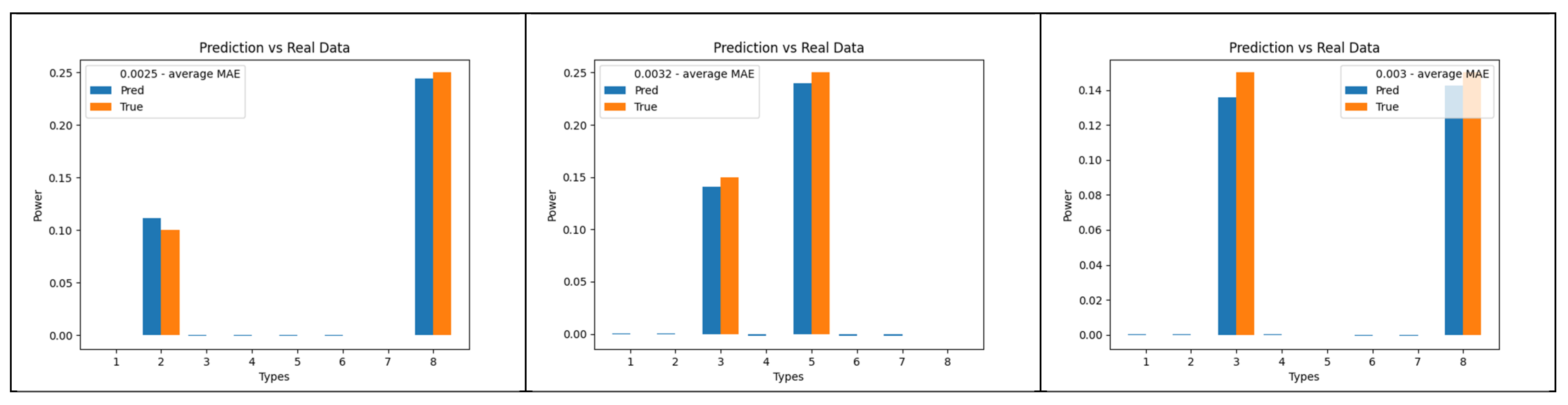
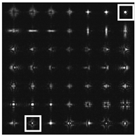
c11 = 0.20, c20 = 0.30 | c11 = 0.20, c22 = 0.30 | c22 = 0.15, c33 = 0.10 |
c42 = 0.20, c33 = 0.15 | c44 = 0.20, c42 = 0.25 | c44 = 0.25, c22 = 0.20 |
c11 = 0.20, c20 = 0.30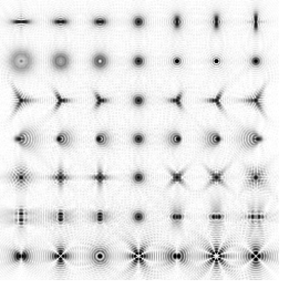 | c11 = 0.20, c22 = 0.30 | c22 = 0.15, c33 = 0.10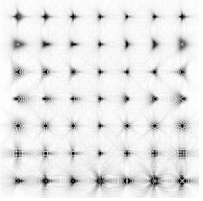 |
c42 = 0.20, c33 = 0.15 | c44 = 0.20, c42 = 0.25 | c44 = 0.25, c22 = 0.20 |
| = −0.5 | = −0.3 | = −0.2 |
|---|---|---|
 |  |  |
| = 0.2 | = 0.3 | = 0.5 |
|---|---|---|
 |  |  |
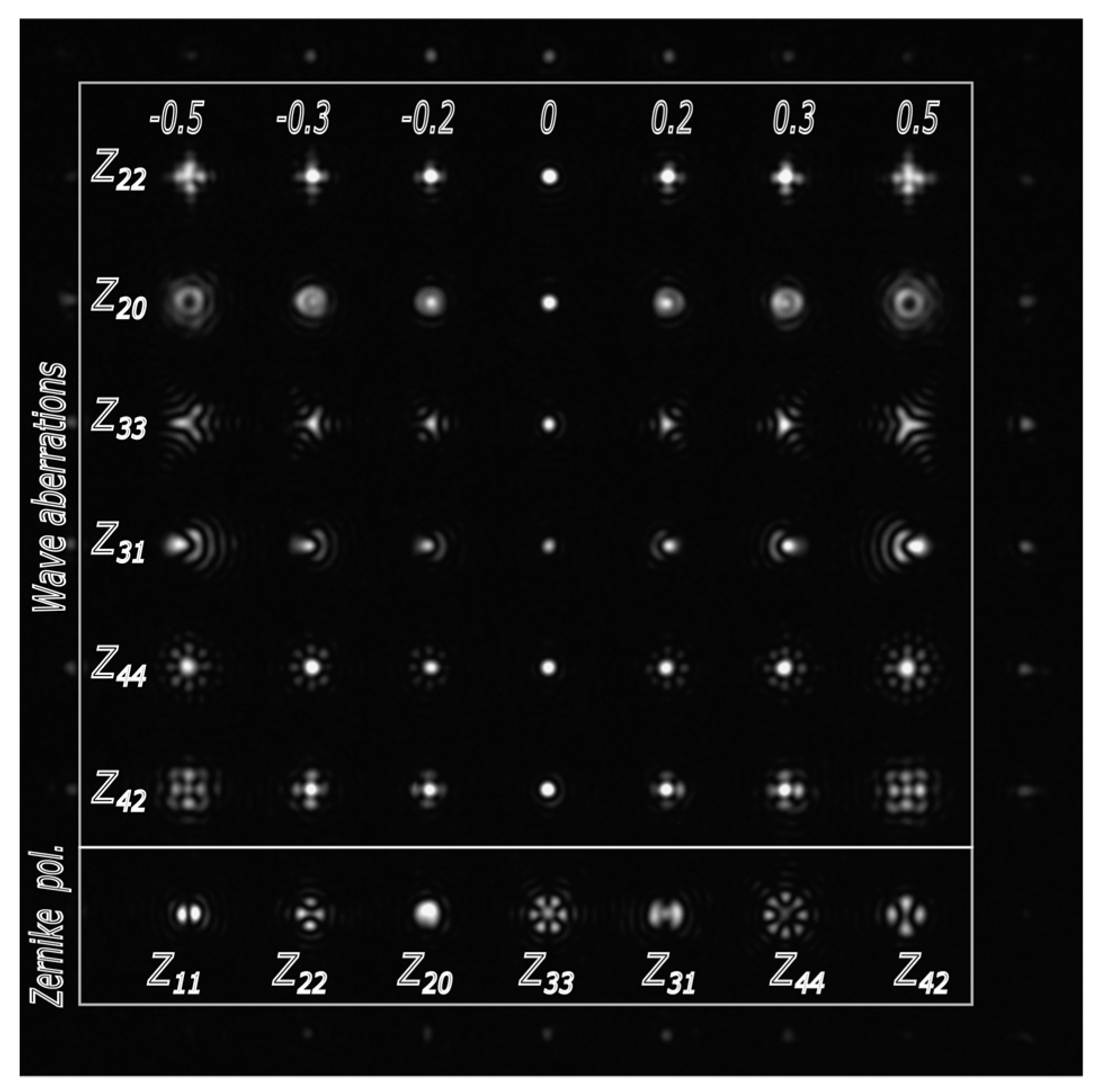
| (n, m) | ||
|---|---|---|
| (2, 0) = 0.20 | 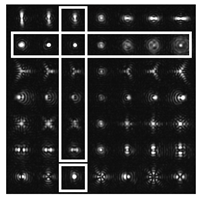 | 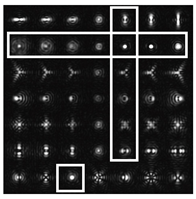 |
| (3, 3) = 0.25 |  |  |
| (3, 1) = 0.45 |  | 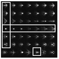 |
| (4, 4) = 0.15 | 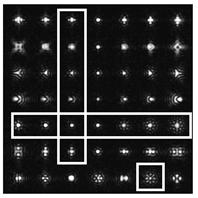 | 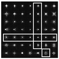 |
| (4, 2) = 0.15 | 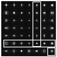 |  |
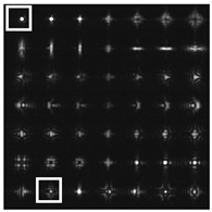
c11 = 0.20, c20 = 0.30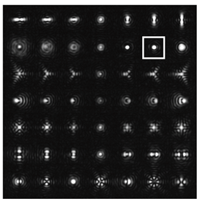 | c11 = 0.20, c22 = 0.30 | c22 = 0.15, c33 = 0.10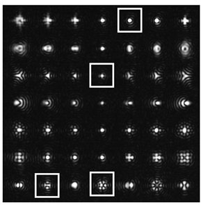 |
c42 = 0.20, c33 = 0.15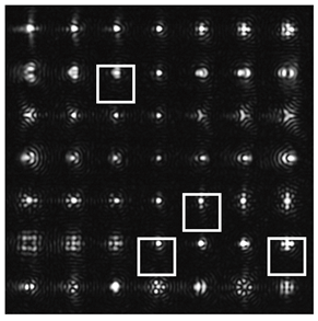 | c44 = 0.20, c42 = 0.25 | c44 = 0.25, c22 = 0.20 |
Disclaimer/Publisher’s Note: The statements, opinions and data contained in all publications are solely those of the individual author(s) and contributor(s) and not of MDPI and/or the editor(s). MDPI and/or the editor(s) disclaim responsibility for any injury to people or property resulting from any ideas, methods, instructions or products referred to in the content. |
© 2025 by the authors. Licensee MDPI, Basel, Switzerland. This article is an open access article distributed under the terms and conditions of the Creative Commons Attribution (CC BY) license (https://creativecommons.org/licenses/by/4.0/).
Share and Cite
Khorin, P.A.; Dzyuba, A.P.; Chernykh, A.V.; Butt, M.A.; Khonina, S.N. Application of Machine Learning Methods for Identifying Wave Aberrations from Combined Intensity Patterns Generated Using a Multi-Order Diffractive Spatial Filter. Technologies 2025, 13, 212. https://doi.org/10.3390/technologies13060212
Khorin PA, Dzyuba AP, Chernykh AV, Butt MA, Khonina SN. Application of Machine Learning Methods for Identifying Wave Aberrations from Combined Intensity Patterns Generated Using a Multi-Order Diffractive Spatial Filter. Technologies. 2025; 13(6):212. https://doi.org/10.3390/technologies13060212
Chicago/Turabian StyleKhorin, Paval. A., Aleksey P. Dzyuba, Aleksey V. Chernykh, Muhammad A. Butt, and Svetlana N. Khonina. 2025. "Application of Machine Learning Methods for Identifying Wave Aberrations from Combined Intensity Patterns Generated Using a Multi-Order Diffractive Spatial Filter" Technologies 13, no. 6: 212. https://doi.org/10.3390/technologies13060212
APA StyleKhorin, P. A., Dzyuba, A. P., Chernykh, A. V., Butt, M. A., & Khonina, S. N. (2025). Application of Machine Learning Methods for Identifying Wave Aberrations from Combined Intensity Patterns Generated Using a Multi-Order Diffractive Spatial Filter. Technologies, 13(6), 212. https://doi.org/10.3390/technologies13060212