Advanced Machine Learning Methods for the Prediction of the Optical Parameters of Tellurite Glasses

Abstract

This study evaluates the predictive performance of advanced machine learning models, including DeepBoost, XGBoost, CatBoost, RF, and MLP, in estimating the Ω₂, Ω₄, and Ω₆ parameters based on a comprehensive set of input variables. Among the models, DeepBoost consistently demonstrated the best performance across the training and testing phases. For the Ω₂ prediction, DeepBoost achieved an R² of 0.974 and accuracy of 99.895% in the training phase, with corresponding values of 0.971 and 99.902% in the testing phase. In comparison, XGBoost ranked second with an R² of 0.929 and accuracy of 99.870% during testing. For Ω₄, DeepBoost achieved a training phase R² of 0.955 and accuracy of 99.846%, while the testing phase results included an R² of 0.945 and accuracy of 99.951%. Similar trends were observed for Ω₆, where DeepBoost obtained near-perfect training phase results (R² = 0.997, accuracy = 99.968%) and testing phase performance (R² = 0.994, accuracy = 99.946%). These findings are further supported by violin plots and correlation analyses, underscoring DeepBoost’s superior predictive reliability and generalization capabilities. This work highlights the importance of model selection in predictive tasks and demonstrates the potential of machine learning for capturing complex relationships in data.

1. Introduction

The Judd–Ofelt (JO) theory has received a great deal of interest due to its wide range of applications in materials science and chemistry, along with their numerous academic issues. Such uses include solid-state lasers [1,2] thermal sensors [3,4], optical amplifiers, upconversion [5], and diverse biological contexts [6,7]. One of the main uses of the JO theory in this application, as in many others, is to provide a description of the optical properties of materials [8]. These properties may include characteristics such as transition probability, branching ratio, and emission cross-section.

The JO theory provides significant insights into the structure of glass and the environment of the rare earth (RE), since the values of the parameters Ω_t (t = 2, 4, and 6) are sensitive to variations of the RE site symmetry and of the RE-O covalency. The Ω₂ parameter describes the ligand field asymmetry of the local RE environment [9,10,11] and/or is proportional to the degree of bond covalency for RE-O [12]. In contrast, the JO intensity parameters Ω₄ and Ω₆ display the viscosity and dielectric properties of the glass matrix [13,14].

Although the JO theory exhibits mathematical elegance and physical utility, it presents a challenging framework not only in its understanding but also in its use. Similar to numerous theories in this field, it requires a sufficient depth of knowledge of solid-state physics and quantum mechanics. Additionally, the glass matrix under consideration for the calculation of the JO intensity parameters and its subsequent characterizations are highly specialized. Consequently, the combination of restrictions on the materials’ preparation, the measurement methods, the subsequent calculations, and the final interpretation makes JO theory elegant but frequently unapproachable. In this respect, given the breadth of applications that have emerged even despite the many limitations, it stands to reason that a more accessible method for obtaining the same or similar information would have very important implications for many scientific actions: for instance, how the three JO parameters could be predicted in the absence of spectral measurements and their corresponding mathematical calculations.

Predicting the relationship between composition and properties plays a crucial role in the developing of novel compositions. The developing physics-based models for predicting the properties in glasses remain a significant challenge that need to be addressed. An alternative method to address these challenges is to employ data-based modeling methods including machine learning [9,10,15]. These techniques rely on accessible data to develop models that capture the hidden trends in the relationships between input and output. In the field of material informatics, ML is employed for various applications, including the development of interatomic potentials [11,16,17], the predicting of novel materials and composites [18,19], the prediction of the composition–property relationship [10,15,20,21], and the development of the energy landscape [22]. Specifically, ML has been successfully used in oxide glasses for predicting a wide range of equilibrium and nonequilibrium composition–property relationships, including the liquidus temperature [9], solubility [20], glass transition temperature [15], stiffness [23], and dissolution kinetics [10].

This research leverages powerful machine learning models including XGBoost, LightGBM, GWO-XGBoost, and GWO-LightGBM to estimate the JO parameters in Er³⁺-doped tellurite glasses. Er³⁺-doped tellurite glass has received a great deal of interest in recent years because of its optical and chemical properties [24]. Their high linear and nonlinear refractive indices, relatively low-phonon energy spectra, a low bonding strength of Te-O, chemical durability, and low glass transitions make them good candidates for fiber laser and 1.5 μm broadband optical amplifier applications [24].

The experimental oscillator strengths ($f_{exp}$) of the f-f induced electric dipole transitions of the various absorption bands are determined by measuring the integral area of the corresponding absorption transitions using the Judd–Ofelt theory [13,14] and the following equation:

$$f_{exp}={\displaystyle \frac{2.303m{c}^2}{N\pi e^2}}\int \epsilon \left(v\right)dv=4.318\times {10}^{-9}\int \epsilon \left(v\right)dv$$

(1)

where $m$ and $e$ are the electron mass and electron charge, respectively; $c$ is the light velocity; $N$ is the Avogadro’s number; and ν is the transition energy (in cm⁻¹). The oscillator strengths ($f_{cal}$) for each absorption transition of the rare-earth ions within the 4f configuration were calculated through the following equation:

$$f_{cal}=\left[{\displaystyle \frac{8{\pi }^{2}mcv}{3h\left(2J+1\right)}}\right]\left[{\displaystyle \frac{{\left(n^2+2\right)}^2}{9n}}\right]\times {\displaystyle \sum }_{t=2,4,6}{\Omega }_t{\left(\Psi J\Vert U^t\Vert {\Psi }^{\prime }{J}^{\prime }\right)}^2$$

(2)

where n is the refractive index; J is the total angular momentum of the ground state; ${\Omega }_t$ ($t$ = 2, 4, and 6) are the Judd–Ofelt intensity parameters, which are used to characterize the metal–ligand band in the host matrix; and $\Vert U^t{\Vert }^2$ is the square reduced matrix elements of the unit tensor operator. The square reduced matrix elements $\Vert U^t{\Vert }^2$ for this present work were obtained from the reported literature [10].

The JO intensity parameters are host-dependent and play a vital role in investigating the glass structure and transition rates of the RE ion energy levels. The Ω₂ JO parameter is related to the covalency and symmetry of the ligand field around the rare-earth ions [15]. The Ω₄ and Ω₆ parameters explore bulk properties like viscosity, the dielectric constant, and the vibronic transitions around the rare-earth ions [9].

Traditional physics-based models, such as those derived from the Judd–Ofelt theory, have been extensively used to predict the optical parameters of rare-earth-doped glasses. These models rely heavily on detailed knowledge of the material’s atomic structure and the interactions between the rare-earth ions and the glass matrix. While they provide valuable insights into the optical properties of the materials, the process often involves complex calculations and assumptions that may not capture the full range of material behaviors, particularly in heterogeneous or poorly characterized systems.

In contrast, ML models, such as DeepBoost, XGBoost, and CatBoost, offer the advantage of data-driven predictions that can account for complex, nonlinear relationships in the data without relying on predefined physical models. These models excel at handling large, multi-dimensional datasets, which may be difficult to interpret using traditional physics-based approaches. Our study demonstrates that ML models, particularly DeepBoost, outperform conventional methods in terms of predictive accuracy and computational efficiency, making them a promising alternative for predicting the optical parameters in materials science. Moreover, ML approaches require fewer domain-specific assumptions, making them applicable to a broader range of materials and conditions where conventional models may not be easily adapted. While traditional models remain invaluable for understanding fundamental principles, ML methods complement them by providing more flexible, scalable, and efficient solutions for predicting material properties.

2. Experimental Procedure

While substantial progress has been made in leveraging machine learning techniques for predictive modeling, significant gaps remain in the systematic evaluation and application of advanced algorithms like DeepBoost, XGBoost, and CatBoost for specific parameters such as Ω₂, Ω₄, and Ω₆. Existing studies often rely on traditional modeling approaches or simpler machine learning models, which fail to capture the intricate nonlinear relationships present in complex datasets with the same level of accuracy and robustness. Moreover, the current literature lacks a detailed comparative analysis of these advanced boosting algorithms in the context of multi-parameter prediction tasks. This creates uncertainty regarding their relative strengths, limitations, and applicability to real-world scenarios. Additionally, most studies do not provide a comprehensive assessment of computational efficiency alongside predictive performance, an essential aspect for the practical deployment of machine learning models in industrial and scientific domains. This study addresses these gaps by introducing a rigorous evaluation framework for these algorithms, emphasizing both accuracy and computational efficiency. By doing so, it provides critical insights into their suitability for modeling Ω₂, Ω₄, and Ω₆, offering a novel contribution to the field and setting the stage for further advancements in machine learning-driven predictive analytics.

In this study, a significant portion of the scientific literature related to the experimental calculation of the three JO parameters (Ω₂, Ω₄, and Ω₆) in erbium-doped tellurite glasses was examined. The final review involved 26 scientific papers, which corresponded to 70 unique types of tellurite glasses doped with erbium [25,26,27,28,29,30,31,32,33,34,35,36,37,38,39,40,41,42,43,44,45,46,47,48,49,50]. The corresponding JO parameters and the percentage of oxide compositions for each glass were determined using stoichiometry (

Table 1. Descriptive statistics of the effective parameters and ${\Omega }_t \left(t=2, 4, \mathrm{and} 6\right)$.

Type	Parameter	Mean	Median	Standard Deviation	Minimum	Maximum
Input	TeO2	46.483	45	23.523	0	80
	SrO	0.857	0	2.820	0	10
	P2O5	1.786	0	7.325	0	35
	CaO	1.404	0	5.314	0	25.9
	CaF2	1.571	0	3.666	0	10
	K2O	1.929	0	5.057	0	15
	Bi2O3	0.963	0	3.002	0	15
	TiO2	0.014	0	0.064	0	0.4
	B2O3	23.377	28.25	24.307	0	79.5
	LiO2	2.361	0	6.457	0	25
	CdF2	0.757	0	3.205	0	18
	WO3	4.679	0	11.462	0	39.92
	ZnO	5.271	0	7.437	0	20
	MgO	3.357	0	6.063	0	15
	Na2O	4.193	0	6.032	0	19
	Er2O3	1.119	1	1.332	0.01	10
Output	Ω2	5.937	5.98	2.457	1.95	11.99
	Ω4	1.847	1.645	0.958	0.171	5.39
	Ω6	1.590	1.62	0.747	0.37	3.54

summarizes the data and the synthesized data).

3. Research Significance

This study is significant as it advances the application of cutting-edge machine learning models—DeepBoost, XGBoost, and CatBoost—in accurately predicting the Ω₂, Ω₄, and Ω₆ parameters, which are crucial in various scientific and industrial domains. The research provides a comprehensive comparison of these algorithms, highlighting their ability to model complex, nonlinear relationships with high precision. By achieving R² values exceeding 0.99 and error metrics such as RMSE and MAPE at remarkably low levels, this study sets a benchmark for predictive modeling in the field. The findings demonstrate the transformative potential of these models in fields like materials science, structural engineering, and environmental management, where accurate parameter predictions are critical for optimizing designs, processes, and resource utilization. Furthermore, the detailed evaluation methodology presented here establishes a framework for future research aiming to adopt advanced machine learning techniques for predictive analytics, fostering a more data-driven and efficient approach to problem-solving. By addressing computational efficiency and prediction reliability, this work also contributes to enhancing real-world applicability, bridging the gap between theoretical advancements and practical implementation in data-driven domains.

4. Data Presentation

This research investigates a substantial segment of the scientific literature concerning the experimental determination of the three JO parameters (Ω₂, Ω₄, and Ω₆) in RE-doped tellurite glasses. The concluding review encompassed scholarly articles [25,26,27,28,29,30,31,32,33,34,35,36,37,38,39,40,41,42,43,44,45,46,47,48,49,50], which related to 70 unique varieties of Er³⁺-doped tellurite glasses. The relevant JO parameters and the percentage of oxide compositions for each glass were established using stoichiometry.

The dataset used in this study includes a comprehensive set of input and output parameters relevant to the analysis of chemical compositions and their effects on the output indices (Ω₂, Ω₄, and Ω₆). Table 1 provides a detailed summary of the descriptive statistics for all the parameters involved. For each parameter, the key statistical metrics are reported, including the mean, median, standard deviation, and minimum and maximum values. Among the input parameters, the oxide compositions (e.g., TeO₂, SrO, P₂O₅, CaO, and CaF₂) and other chemical compounds (e.g., K₂O, Bi₂O₃, and TiO₂) show considerable variability, reflecting the diverse chemical nature of the dataset. For example, TeO₂ exhibits a wide range of values, with a mean of 46.483 and a standard deviation of 23.523, indicating significant variation across the samples. Similarly, other components, such as SrO and P₂O₅, have skewed distributions, as evidenced by their median values being notably different from the mean. The maximum values of certain parameters, such as P₂O₅ (35) and B₂O₃ (79.5), demonstrate that some samples contain extraordinarily high concentrations of specific compounds, which may influence the output indices significantly. The output parameters (Ω₂, Ω₄, and Ω₆) represent specific indices calculated based on the input compositions. These indices display unique statistical characteristics. For instance, Ω₂ has a mean of 5.937 and a standard deviation of 2.457, suggesting moderate variability. In contrast, Ω₄ and Ω₆ show lower mean values of 1.847 and 1.590, respectively, with relatively smaller standard deviations. These indices provide a quantitative measure of the system’s behavior, which is further analyzed in the correlation matrix (Figure 1). The descriptive statistics serve as a foundation for the subsequent correlation and modeling analysis. By understanding the variability and distribution of the input and output parameters, researchers can better assess the relationships and interactions within the dataset, ultimately enhancing the interpretability of the findings.

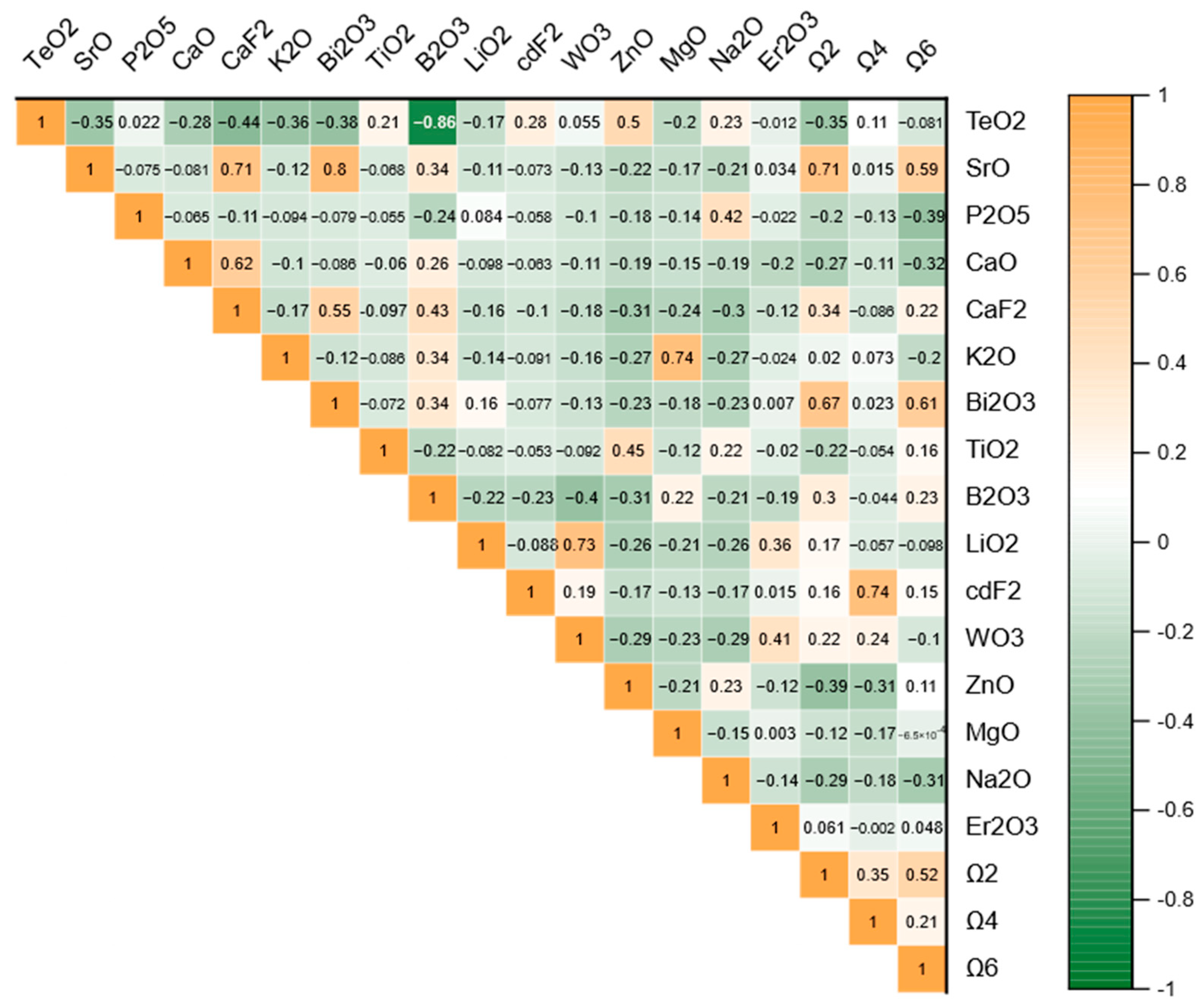
The correlation matrix depicted in Figure 1 illustrates the relationships between the input parameters and the output indices (Ω₂, Ω₄, and Ω₆). The matrix displays the Pearson correlation coefficients, which quantify the linear relationship between pairs of variables. Values closer to 1 or −1 indicate stronger positive or negative correlations, respectively, while values near zero suggest weak or no correlations. Several key patterns can be observed from the matrix. The parameter TeO₂ shows moderate negative correlations with output indices such as Ω₂ (−0.353) and Ω₆ (−0.081), indicating that higher concentrations of TeO₂ might slightly reduce these indices. In contrast, SrO exhibits a strong positive correlation with Ω₂ (0.711) and a moderate positive correlation with Ω₆ (0.591), suggesting its significant influence on these outputs. Interestingly, Bi₂O₃ is also strongly correlated with Ω₂ (0.674) and Ω₆ (0.605), highlighting its potential role in determining the system’s characteristics. Some input parameters demonstrate notable interdependence. For example, CaF₂ and SrO are strongly positively correlated (0.709), as are MgO and K₂O (0.743). These relationships may indicate underlying chemical or physical interactions between these compounds. Additionally, the weak or negative correlations observed between some parameters, such as B₂O₃ and ZnO (−0.307), suggest minimal interaction or opposing trends. The output indices Ω₂, Ω₄, and Ω₆ exhibit distinct correlations with the input parameters. Ω₂ shows significant positive relationships with several variables, including SrO, Bi₂O₃, and CaF₂, while Ω₄ demonstrates strong positive correlations with CdF₂ and moderate negative correlations with MgO and ZnO. Ω₆, on the other hand, is positively influenced by Bi₂O₃ and SrO but shows weaker interactions with many other parameters. Figure 1 is critical for identifying the dominant factors influencing the output indices and serves as a guide for further modeling and analysis. The insights derived from the correlation matrix provide a valuable foundation for predictive modeling, enabling the identification of the most impactful parameters and their interactions.

5. Methods

5.1. Multilayer Perceptron (MLP)

There are numerous successive layers of neurons that make up a MLP, which is a form of artificial neural network (ANN). These layers comprise an input layer, one or more hidden layers, and an output layer. Each layer is completely coupled to the layer that comes after it. As a result of its capacity to represent complex and nonlinear interactions between data points, multilayer perceptrons, also known as MLPs, are widely used for supervised learning tasks such as classification and regression [51]. MLPs are able to extract nonlinear features with ease because of the utilization of nonlinear activation functions in the hidden layers. This capability makes it possible for MLPs to facilitate the representation of complicated data and the transfer of data to higher dimensional space. According to Equation (3), the training approach for a multilayer perceptron makes use of the backpropagation algorithm. This algorithm is responsible for refining a loss function by adjusting the weights in accordance with the gradients that are produced via error propagation. For the purpose of this investigation, the Sigmoid function (Equation (4)) and the mean squared error (MSE) loss function (Equation (5)) were applied.

$$w\leftarrow w-\eta {\displaystyle \frac{\partial L}{\partial w}}$$

(3)

$$\sigma \left(x\right)={\displaystyle \frac{1}{1+e^{-x}}}$$

(4)

$$L=-{\displaystyle \frac{1}{N}}{\displaystyle \sum }_{i=1}^N\left[y_{i}log\left({\widehat{y}}_i\right)+\left(1-y_i\right)log\left(1-{\widehat{y}}_i\right)\right]$$

(5)

The activation functions used in the hidden layers are Rectified Linear Units (ReLUs), which were chosen due to their ability to efficiently capture nonlinearities and improve the model’s convergence speed. The output layer employs a linear activation function, as we are dealing with a regression problem where continuous values are predicted. To prevent overfitting and enhance generalization, we employed several regularization techniques. Moreover, dropout regularization with a dropout rate of 0.2 was applied to the hidden layers to further prevent overfitting and encourage the model to generalize better. The model was trained using the backpropagation algorithm with the Adam optimizer, which is known for its efficiency in terms of both memory and computation. The learning rate was set to 0.001, and the model was trained for 500 epochs with early stopping to avoid overfitting. The mean squared error (MSE) loss function was used to optimize the model’s predictions.

5.2. Extreme Gradient Boosting (XGBoost)

This is analogous to the ensemble technique, a kind of machine learning algorithm. To provide a stronger and more accurate forecast, the ensemble uses a number of different basic regression models, sometimes known as decision trees. Boosting is the technique of fitting these numerous models sequentially [52]. To boost, you train a series of rudimentary models, or “weak learners”, one after the other, with the idea that one model may learn from the mistakes of the others. A single or double branch is used to construct these basic models. By averaging the forecasts from all the basic models, the final prediction considers all of them. With its many hyperparameters that can be adjusted for a personalized fit, this model excels at handling complicated and huge datasets. By using the XGBoost XGBRegressor package, this concept is put into action [53]. The following is a definition of this pattern:

$${\hat{y}}_i={\displaystyle \sum }_{k=1}^K{f}_k\left(x_i\right)$$

(6)

The value that is anticipated to be used for updating the i-th building is denoted by the symbol ${\hat{y}}_i$, where f_k represents the prediction of the k-th tree for building x_i and K represents the total number of trees that are included in the model. With each additional tree that is built, the accuracy of the prediction steadily increases. The model optimizes the objective function L_ϕ, which results in a reduction in the amount of prediction error:

$$L\left(\varphi \right)={\displaystyle \sum }_{i=1}^{n}l\left(y_i,{\hat{y}}_i\right)+{\displaystyle \sum }_{k=1}^K\mathsf{\Omega }\left(f_k\right)$$

(7)

where the regularization term and the loss function are represented by Ω(f_k) and $l\left(y_i,{\hat{y}}_i\right)$, respectively. The difference between the actual update demand, denoted by y_i, and the value that was expected, denoted by ${\hat{y}}_i$, is what the loss function measures. The regularization term is responsible for controlling the complexity of the model in order to avoid overfitting in the urban renewal prediction. The formula for the regularization term is presented as follows:

$$\mathsf{\Omega }\left(f_k\right)={\rm Y}T+{\displaystyle \frac{1}{2}}\gamma {{\displaystyle \sum }}_{j=1}^T{w}_j^2$$

(8)

In this equation, the parameters ${\rm Y}$ and $\gamma$ represent regularization, $T$ represents the number of leaf nodes, and $w_j$ represents the weight of the leaf.

The hyperparameter tuning process for the XGBoost model was performed to optimize its performance and ensure good generalization to unseen data. The key hyperparameters were tuned, including the learning rate (η), which controls the step size during optimization, with values tested in the range of 0.01 to 0.1; the maximum depth (max_depth) of each tree, ranging from 3 to 10, which controls model complexity; the number of estimators (n_estimators), tested from 50 to 500, which defines the number of boosting rounds; the subsample ratio, ranging from 0.5 to 1.0, which dictates the fraction of samples used for fitting each individual tree; and the colsample_bytree parameter, controlling the fraction of features used for each tree, optimized in the range of 0.3 to 1.0. The optimization was carried out using grid search, where we exhaustively tested combinations of these hyperparameters within predefined grids. The best configuration was selected based on the model’s performance on the validation set, where the mean squared error (MSE) was used as the objective function to minimize. To further prevent overfitting and enhance model performance, early stopping was implemented during training, with the training halting if the performance on the validation set did not improve for 100 consecutive rounds. In this model, the optimal set of hyperparameters obtained through the grid search resulted in the best model configuration for predicting the optical parameters of the tellurite glasses.

5.3. Random Forest Regressor (RF)

One example of a mathematical method is one that generates several decision trees by using random subsets of the characteristics from the training set. A random portion of the training data and a random subset of the predictor variables are introduced into each decision tree throughout the training process. For the purpose of determining the ultimate forecast, each decision tree generates a unique prediction, and the final output is computed by taking the average of the predictions generated by all of the trees [54]. The essence of the Random Forest resides in the fact that any single decision tree may be subject to bias or mistakes; nevertheless, when taken as a whole, the trees have the potential to provide a more accurate forecast than any one tree could ever produce on its own. To further enhance the model’s generalizability and decrease overfitting, it is recommended to train each tree with random features and use a random subset of the training data [55]. It is possible to create this model in Python 3.12.7 by using the Random Forest Regressor module that is part of the sklearn ensemble distribution.

5.4. CatBoost

As a high-performance Gradient Boosting technique for categorical data, CatBoost is an open-source algorithm [56]. It is capable of handling categorical data, which eliminates the need for preprocessing techniques such as label encoding or one-hot operation [57]. CatBoost is a useful strategy for use with smaller datasets since it employs statistical methods and target-based encoding to decrease the amount of overfitting that occurs. In addition, it functions well with the default settings, which eliminates the need for hyperparameter customization [58]. It is the default behavior of CatBoost to produce one thousand six-level binary two-leaf trees. Because the calculation of the automated learning rate is limited by the characteristics of the training dataset and the number of iterations, automatic learning is the most efficient method. Training may be sped up by increasing the learning rate and decreasing the number of iterations. A model depth of (6, 8, and 10), learning rate of (0.01, 0.1, and 0.2), and model iterations of (100 and 200) were the hyperparameters used to train the CatBoost model and acquire the desired parameters.

6. Model Evaluation

Model evaluation is a critical step in the development and implementation of predictive models, as it provides a comprehensive assessment of their performance and reliability. The primary objective of this process is to determine the model’s ability to generalize effectively to unseen data while ensuring that it meets the desired accuracy and robustness criteria. Evaluating models is essential to identify the most suitable algorithm for a specific problem, especially in complex predictive tasks where multiple models, such as MLP, CatBoost, XGBoost, RF, and DeepBoost, are employed.

In this study, the evaluation process involved the calculation of several performance metrics for each model during both the training and testing phases. Metrics such as the Coefficient of Determination (R²); Variance Accounted For (VAF); a-20 index, Performance Index (PI), and accuracy were employed to evaluate the models based on the literature’s suggestions [59,60,61,62,63,64]. Each metric provides unique insights into the models’ performance. For instance, R² measures the proportion of variance explained by the model, while VAF indicates the degree to which the predicted values align with the observed values. The a-20 index evaluates the percentage of predictions falling within an acceptable range of deviation, and PI combines multiple aspects of prediction accuracy into a single measure. Lastly, accuracy reflects the overall correctness of the predictions.

By evaluating the models across these diverse metrics, this study aims to identify the optimal predictive algorithm for forecasting the Ω₂, Ω₄, and Ω₆ parameters. Such a comprehensive evaluation is not only essential for selecting the best-performing model but also for understanding the strengths and weaknesses of each algorithm, thereby enabling informed decisions in future applications. This rigorous approach ensures that the selected model provides reliable and accurate predictions, which are crucial for addressing the underlying research objectives effectively. The used statistical indices in this study can be formulated as follows [60,62,63,64,65,66,67,68,69,70,71,72]:

$$R^2={\displaystyle \frac{{{\displaystyle \sum }}_{i=1}^n{\left(m_{{\Omega }_i}-{\overline{m}}_{\Omega }\right)}^2-{{\displaystyle \sum }}_{i=1}^n{\left(m_{{\Omega }_i}-P_{{\Omega }_i}\right)}^2}{{{\displaystyle \sum }}_{i=1}^n{\left(m_{{\Omega }_i}-{\overline{m}}_{\Omega }\right)}^2}}$$

(9)

$$VAF=\left(1-{\displaystyle \frac{var\left(m_{{\Omega }_i}-P_{{\Omega }_i}\right)}{var\left(m_{{\Omega }_i}\right)}}\right)\times 100$$

(10)

$$a^{20} index={\displaystyle \frac{m^{20}}{n}}$$

(11)

$$PI=R^2+0.01\times VAF-RMSE$$

(12)

$$ACC=100-{\displaystyle \frac{100}{n}}\times {\displaystyle \sum }_{i=1}^n{\displaystyle \frac{\left|m_{{\Omega }_i}-P_{{\Omega }_i}\right|}{\left(\left|m_{{\Omega }_i}+P_{{\Omega }_i}\right|\right)/2}}$$

(13)

where m signifies the number of data points; and $m_{{\Omega }_i}$, ${\overline{m}}_{\Omega }$, and $P_{{\Omega }_i}$ are, respectively, the measured, anticipated, and average of the real ${\Omega }_t,\left(\mathrm{t}=2, 4, \mathrm{and} 6\right)$ values [67,69,70,73].

Underpinning the success of this evaluation is the preprocessing step of data normalization, which plays a fundamental role in ensuring the models’ reliability and comparability. Normalization adjusts the scale of input features to prevent variables with larger ranges from disproportionately influencing the learning process. This step is particularly critical given the diversity of input features utilized for predicting Ω₂, Ω₄, and Ω₆.

In this study, the min–max normalization technique was employed, which scales each feature to a range of [0, 1] using the following formula:

$$x_i^{norm}={\displaystyle \frac{x_i-x_{min}}{x_{max}-x_{min}}}$$

(14)

Here, x_i represents the original data point, while x_min and x_max denote the minimum and maximum values of the respective feature. This transformation ensures that all features contribute equally to the training process, enhancing the models’ convergence rates and reducing computational inefficiencies.

The normalization process is particularly vital for models such as MLP and DeepBoost, where the scale of inputs significantly impacts the optimization of weights. Moreover, while tree-based models like CatBoost, XGBoost, and RF are less sensitive to feature scaling, normalization was applied uniformly across all the models to ensure consistency and fairness in the evaluation process.

By incorporating normalization, this study guarantees that the comparative analysis of model performance remains unbiased and that the chosen model delivers robust and accurate predictions of Ω₂, Ω₄, and Ω₆. This preprocessing step further underscores the rigor and methodological soundness of the evaluation framework.

To ensure a robust evaluation of the predictive models, the dataset was partitioned into two distinct subsets: a training set and a testing set. This division is a fundamental practice in machine learning to assess the model’s performance on unseen data and to avoid overfitting, where the model performs well on training data but poorly on new data.

In this study, 80% of the available data, corresponding to 56 samples, was allocated to the training set. The training set is used to fit the models, allowing them to learn the underlying patterns and relationships in the data. The remaining 20%, consisting of 14 samples, was designated as the testing set. The testing set serves as an independent dataset to evaluate the model’s generalization ability, providing an unbiased estimate of its predictive performance. Although the data can be partitioned according to various schemes (e.g., 60/40, 70/30, 80/20, and 90/10), in this study the chosen partitioning ratio was selected based on the researcher’s recommendation [74,75,76,77,78,79,80].

The data partitioning was carried out using a random sampling method to ensure that both subsets represent the overall distribution of the dataset. This approach minimizes the risk of introducing selection bias, which could compromise the reliability of the evaluation. Additionally, care was taken to maintain the integrity of the dataset by ensuring that no overlap occurred between the training and testing sets.

By adopting this partitioning strategy, this study guarantees that the models are rigorously evaluated under realistic conditions. The separate evaluation on the testing set provides critical insights into each model’s ability to predict the Ω₂, Ω₄, and Ω₆ parameters accurately and consistently, further reinforcing the validity of the performance comparison.

To gain a deeper understanding of the relationships between the input parameters and the optical properties (Ω₂, Ω₄, and Ω₆), a sensitivity analysis was conducted using the Cosine Amplitude Method (CAM). This method quantifies the strength of the relationship between pairs of effective parameters and their influence on the output variables (Ω_t). The CAM employs the following equation:

$$r_{ij}={\displaystyle \frac{{\displaystyle \sum _{k=1}^m{x}_{ik}.x_{jk}}}{\sqrt{\left({\displaystyle \sum _{k=1}^m{x}_{ik}^2}\right).\left({\displaystyle \sum _{k=1}^m{x}_{jk}^2}\right)}}}$$

(15)

in which r_ij is the intensity impact between x_i (input) and x_j (output).

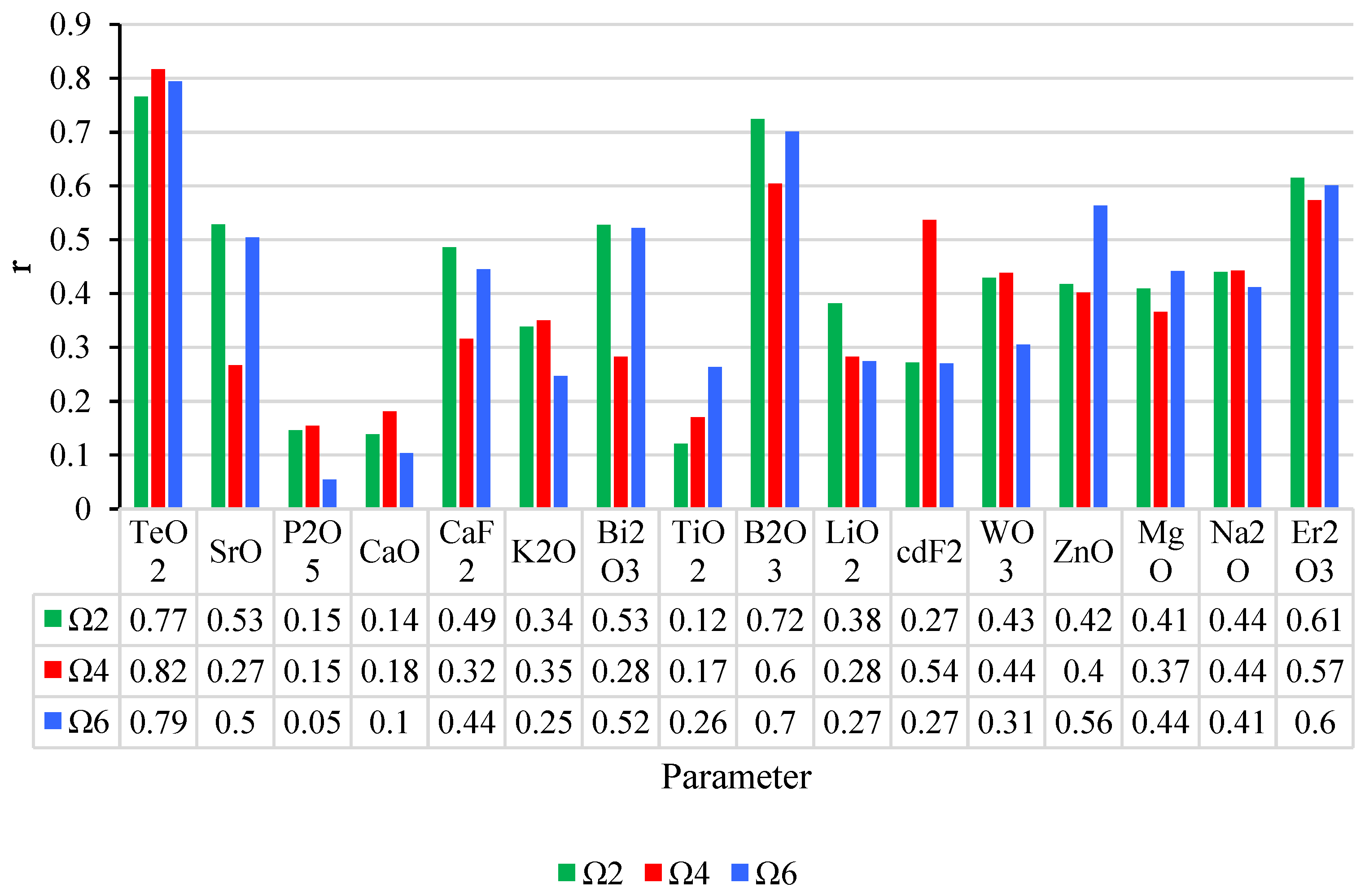
The sensitivity analysis conducted using the Cosine Amplitude Method (CAM) provides valuable insights into the relative importance of the input parameters in influencing the output optical properties, specifically Ω₂, Ω₄, and Ω₆. As shown in Figure 2, the results indicate that certain parameters have a stronger effect on the prediction of these optical properties. For instance, TeO₂ demonstrates a strong influence on Ω₂, with a higher sensitivity value indicating that changes in the TeO₂ concentration have a notable impact on the optical behavior of the material. Similarly, parameters like B₂O₃ and CaF₂ are shown to significantly affect Ω₄ and Ω₆, with their contributions being more pronounced in predicting these parameters. Other parameters, such as ZnO and Na₂O, while still influential, have a relatively weaker effect on the outputs.

7. Results and Discussion

The statistical performance of the models for predicting Ω₂ is detailed in

Table 2. The calculated statistical indicators for the developed models for the prediction of Ω₂.

Model	Training Phase					Testing Phase
	R2	VAF	PI	Accuracy	a-20	R2	VAF	PI	Accuracy	m20
MLP	0.907	90.382	1.055	99.877	0.852	0.869	86.708	0.389	99.830	0.786
CatBoost	0.920	90.743	1.103	99.886	0.907	0.887	88.681	0.605	99.874	0.714
XGBoost	0.931	92.344	1.142	99.889	0.852	0.929	87.468	0.722	99.870	0.786
RF	0.920	91.455	1.224	99.895	0.889	0.905	87.800	0.262	99.839	0.786
DeepBoost	0.974	96.704	1.297	99.895	0.944	0.971	96.282	1.108	99.902	0.929

and

Table 3. Rating the statistical indicators to select the best developed model for the prediction of Ω₂.

Model	Training Phase					Testing Phase					Total Rate	Model Rank
	R2	VAF	PI	Accuracy	a-20	R2	VAF	PI	Accuracy	a-20
MLP	1	1	1	1	1	1	1	2	1	2	12	5
CatBoost	2	2	2	2	4	2	4	3	4	1	26	4
XGBoost	4	4	3	3	1	4	2	4	3	2	30	2
RF	3	3	4	5	3	3	3	1	2	2	29	3
DeepBoost	5	5	5	4	5	5	5	5	5	5	49	1

. These tables reveal distinct trends in the accuracy and reliability of each model during the training and testing phases.

During the training phase, DeepBoost emerged as the most effective model, achieving the highest R² value of 0.974, indicating that it explains 97.4% of the variance in the training data. This was corroborated by its VAF score of 96.704, further emphasizing its robust fitting ability. DeepBoost’s Performance Index (PI) of 1.297 and accuracy of 99.895 demonstrate its ability to make precise predictions. Additionally, the a-20 index, which reflects the proportion of predictions falling within 20% of the observed values, was the highest for DeepBoost (0.944), showcasing its reliability in practical scenarios.

Other models, while competitive, lagged behind DeepBoost. XGBoost achieved the second-highest R² (0.931) and VAF (92.344), but its PI (1.142) and accuracy (99.889) were slightly lower. Similarly, CatBoost and RF had R² values of 0.920 and 0.920, respectively, but their a-20 indices (0.907 for CatBoost and 0.889 for RF) were lower than that of DeepBoost. MLP, while showing decent performance (R² = 0.907), had the lowest PI (1.055) and accuracy (99.877), indicating relatively less precise predictions.

The testing phase results reveal that DeepBoost maintained its superior performance. It achieved an R² value of 0.971, VAF of 96.282, and PI of 1.108, all significantly higher than those of the other models. Its accuracy of 99.902 and a-20 index of 0.929 further underscored its strong generalization ability.

In contrast, other models displayed varying degrees of decline in their performance. XGBoost demonstrated relatively strong results, with an R² of 0.929 and a PI of 0.722, but its accuracy (99.870) and a-20 index (0.786) were notably lower than those of DeepBoost. CatBoost performed moderately well, achieving an R² of 0.887 and a PI of 0.605. MLP and RF showed the weakest generalization ability, with R² values of 0.869 and 0.905, respectively, and lower a-20 indices of 0.786.

As shown in Table 3, DeepBoost ranked first across both the training and testing phases, achieving the best total rate of 49. The consistent performance of DeepBoost reflects its ability to balance accuracy and reliability. In contrast, MLP ranked last with a total rate of 12, suggesting its limited effectiveness for predicting Ω₂.

Table 4. The calculated statistical indicators for the developed models for the prediction of Ω₄.

Model	Training Phase					Testing Phase
	R2	VAF	PI	Accuracy	a-20	R2	VAF	PI	Accuracy	m20
MLP	0.899	89.810	1.427	99.785	0.704	0.867	77.344	1.495	99.917	0.929
CatBoost	0.910	90.786	1.488	99.817	0.611	0.882	83.421	1.593	99.936	1.000
XGBoost	0.929	92.857	1.555	99.816	0.778	0.911	88.812	1.697	99.945	1.000
RF	0.919	91.429	1.512	99.831	0.704	0.897	87.325	1.663	99.941	1.000
DeepBoost	0.955	95.171	1.674	99.846	0.741	0.945	93.992	1.787	99.951	1.000

highlights the strong performance of DeepBoost in predicting Ω₄. It achieved the highest R² (0.955), VAF (95.171), and PI (1.674) during the training phase, indicating its exceptional ability to model the data. Its accuracy of 99.846 and a-20 index of 0.741 reinforce its reliability.

Other models, while competitive, demonstrated weaker performances. XGBoost (R² = 0.929, VAF = 92.857) and RF (R² = 0.919, VAF = 91.429) followed DeepBoost, but their PI values (1.555 and 1.512, respectively) were notably lower. CatBoost achieved moderate results (R² = 0.910, VAF = 90.786), while MLP ranked lowest, with an R² of 0.899 and a PI of 1.427.

In the testing phase, DeepBoost continued to dominate, achieving an R² of 0.945, VAF of 93.992, and PI of 1.787. Its accuracy of 99.951 and a-20 index of 1.000 signify its excellent generalization performance.

Other models showed varying levels of success. XGBoost and RF achieved relatively high R² values (0.911 and 0.897, respectively) and competitive accuracy scores (99.945 and 99.941). However, their PI and a-20 indices were lower than those of DeepBoost. CatBoost displayed moderate performance, while MLP again showed the weakest results, with an R² of 0.867 and a PI of 1.495.

As shown in

Table 5. Rating the statistical indicators to select the best developed model for the prediction of Ω₄.

Model	Training Phase					Testing Phase					Total Rate	Model Rank
	R2	VAF	PI	Accuracy	a-20	R2	VAF	PI	Accuracy	a-20
MLP	1	1	1	1	2	1	1	1	1	1	11	5
CatBoost	2	2	2	3	1	2	2	2	2	2	20	4
XGBoost	4	4	4	2	5	4	4	4	4	2	37	2
RF	3	3	3	4	2	3	3	3	3	2	29	3
DeepBoost	5	5	5	5	4	5	5	5	5	2	46	1

, DeepBoost ranked first with a total rate of 46, significantly outperforming other models. MLP ranked last with a total rate of 11, reinforcing its limited capability in predicting Ω₄.

The training phase results for the Ω₆ predictions, shown in

Table 6. The calculated statistical indicators for the developed models for the prediction of Ω₆.

Model	Training Phase					Testing Phase
	R2	VAF	PI	Accuracy	a-20	R2	VAF	PI	Accuracy	m20
MLP	0.927	91.299	1.654	99.847	0.833	0.919	90.801	1.508	99.823	0.714
CatBoost	0.939	93.495	1.695	99.867	0.815	0.924	92.435	1.585	99.872	0.857
XGBoost	0.934	93.322	1.701	99.887	0.870	0.920	90.303	1.515	99.867	0.857
RF	0.953	94.049	1.738	99.880	0.815	0.949	94.783	1.650	99.876	0.786
DeepBoost	0.997	99.681	1.948	99.968	1.000	0.994	99.323	1.870	99.946	1.000

, reveal that DeepBoost excelled with near-perfect values for all the indicators. It achieved an R² of 0.997, VAF of 99.681, and PI of 1.948, alongside an accuracy of 99.968 and an a-20 index of 1.000. These metrics highlight its ability to capture the underlying relationships in the data.

Other models displayed good but less impressive performances. RF followed with an R² of 0.953 and a VAF of 94.049, but its PI (1.738) and a-20 index (0.815) were notably lower. XGBoost and CatBoost achieved similar R² values (0.934 and 0.939, respectively), but their lower PI values (1.701 and 1.695) and a-20 indices (0.870 and 0.815) limited their competitiveness. MLP showed the weakest results, with an R² of 0.927 and a PI of 1.654.

In the testing phase, DeepBoost maintained its superiority, achieving an R² of 0.994, VAF of 99.323, and PI of 1.870. Its accuracy of 99.946 and a-20 index of 1.000 confirmed its exceptional generalization ability.

Other models showed declines in performance compared to the training phase. RF (R² = 0.949) and XGBoost (R² = 0.920) followed DeepBoost, but their PI and a-20 indices were lower. CatBoost and MLP exhibited moderate results, with R² values of 0.924 and 0.919, respectively.

Table 7. Rating the statistical indicators to select the best developed model for the prediction of Ω₆.

Model	Training Phase					Testing Phase					Total Rate	Model Rank
	R2	VAF	PI	Accuracy	a-20	R2	VAF	PI	Accuracy	a-20
MLP	1	1	1	1	3	1	2	1	1	1	13	5
CatBoost	3	3	2	2	1	3	3	3	3	3	26	3
XGBoost	2	2	3	4	4	2	1	2	2	3	25	4
RF	4	4	4	3	1	4	4	4	4	2	34	2
DeepBoost	5	5	5	5	5	5	5	5	5	5	50	1

confirms that DeepBoost achieved the top rank with a total rate of 50. MLP, despite its reasonable accuracy, ranked last with a total rate of 13, highlighting its comparatively weaker predictive performance.

The analyses across Ω₂, Ω₄, and Ω₆ consistently identify DeepBoost as the most effective model. Its exceptional performance in both the training and testing phases underscores its ability to handle complex datasets and provide reliable predictions. Conversely, MLP ranked lowest for all the targets, demonstrating limited utility in this context.

The findings validate the evaluation framework and highlight the importance of model selection in predictive tasks, offering significant implications for similar studies and practical applications.

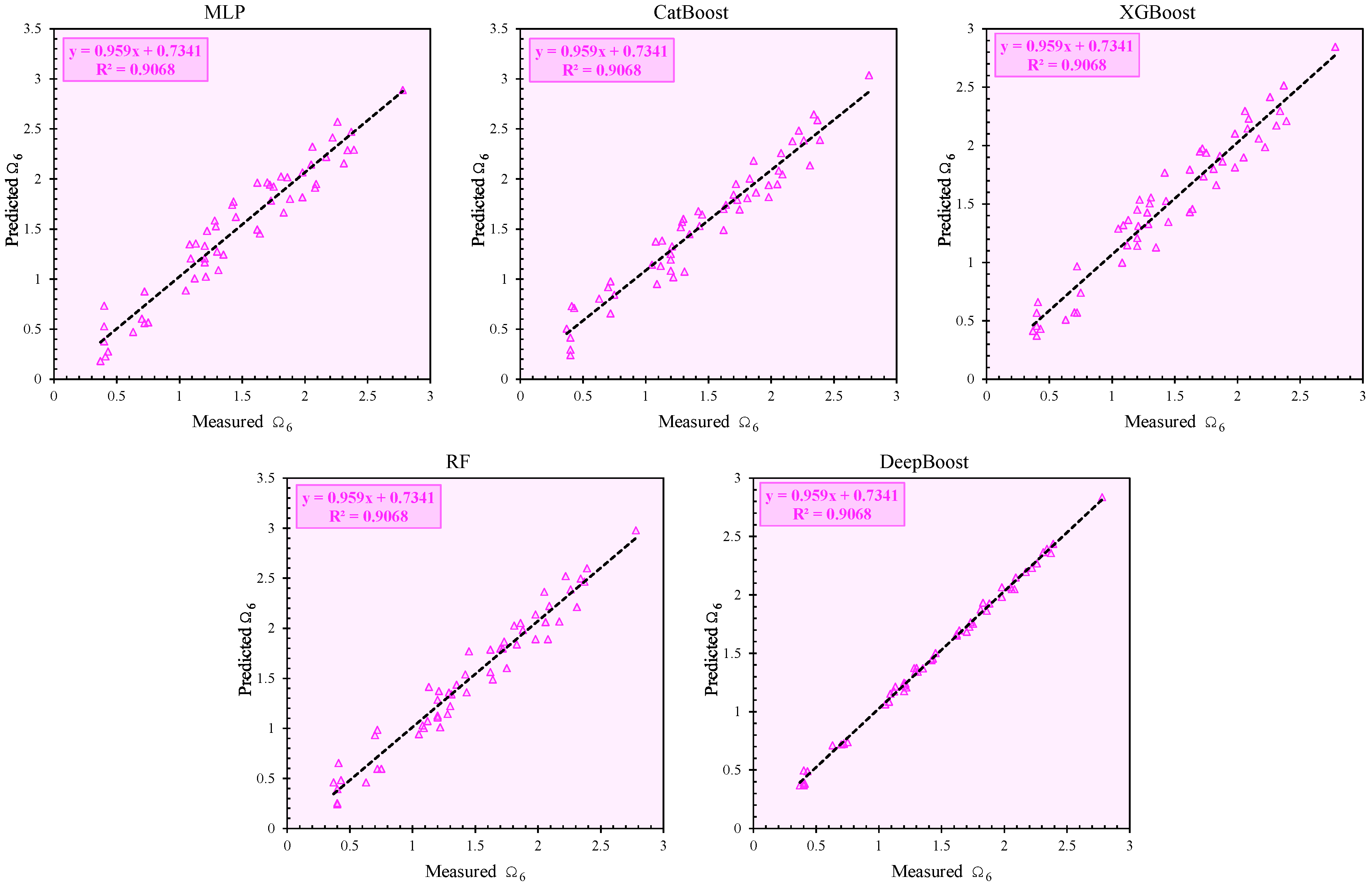
Figure 3, Figure 4, Figure 5, Figure 6, Figure 7 and Figure 8 illustrate the correlation between the measured and predicted values of the target parameters (Ω₂, Ω₄, and Ω₆) for both the training and testing phases. These plots provide a visual assessment of the predictive accuracy of the developed models. In Figure 3 and Figure 4, the measured versus predicted values for Ω₂ during the training and testing phases are shown. The data points cluster tightly around the 45-degree line, indicating a strong correlation and minimal deviation between the observed and predicted values. This highlights the models’ reliability in predicting Ω₂. 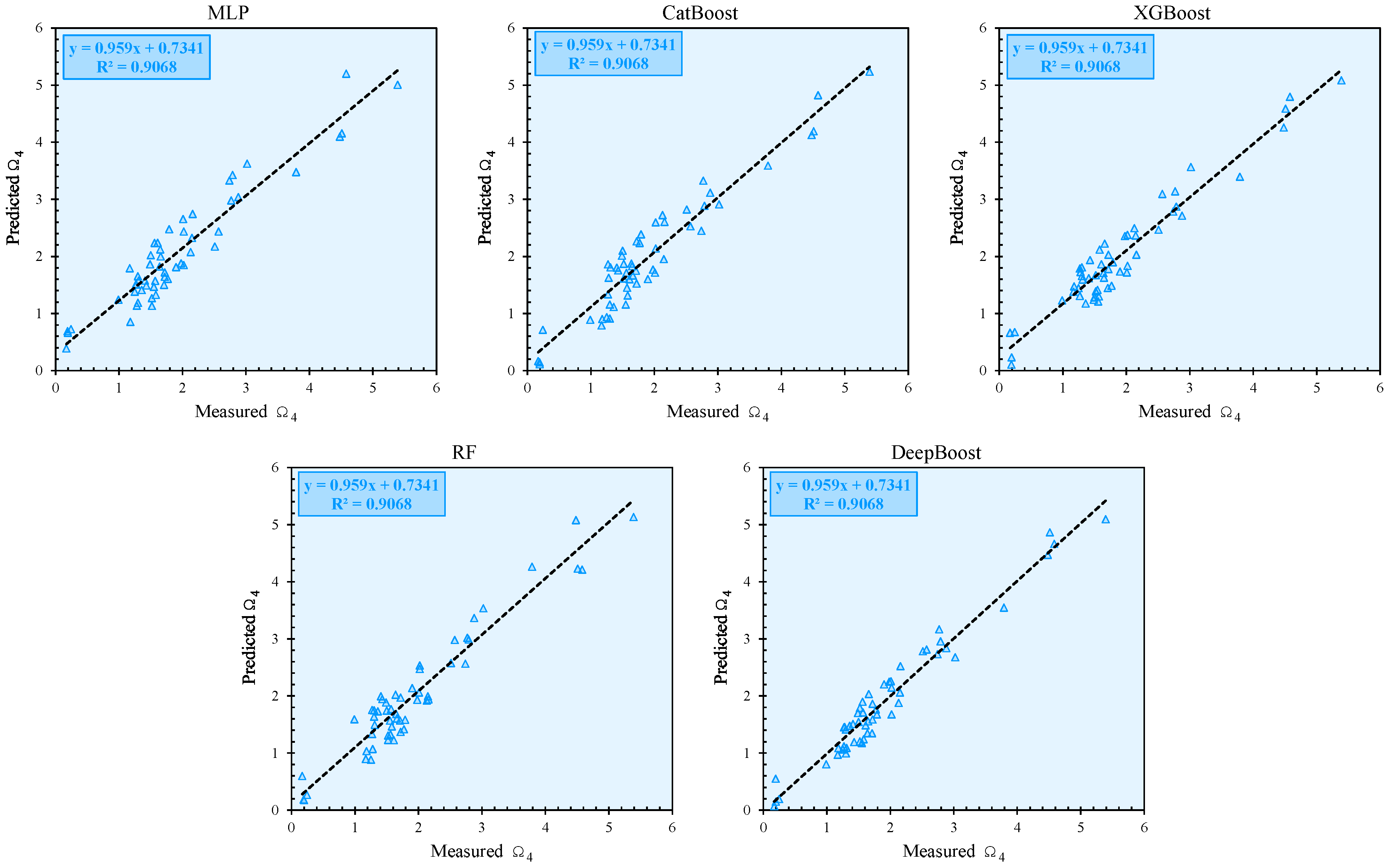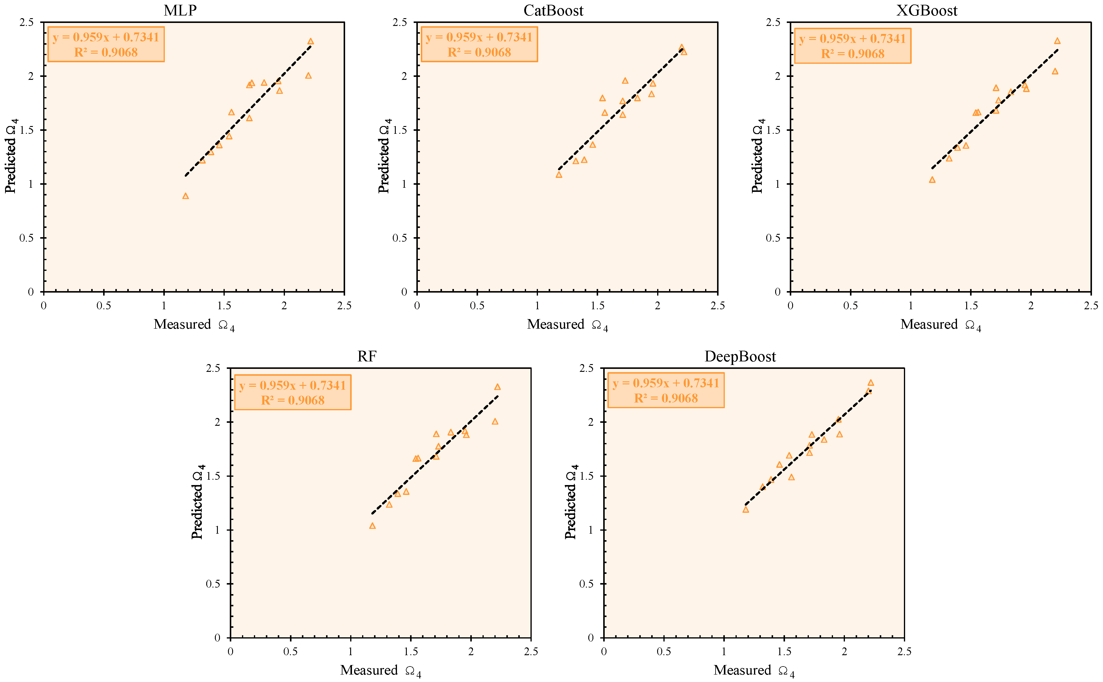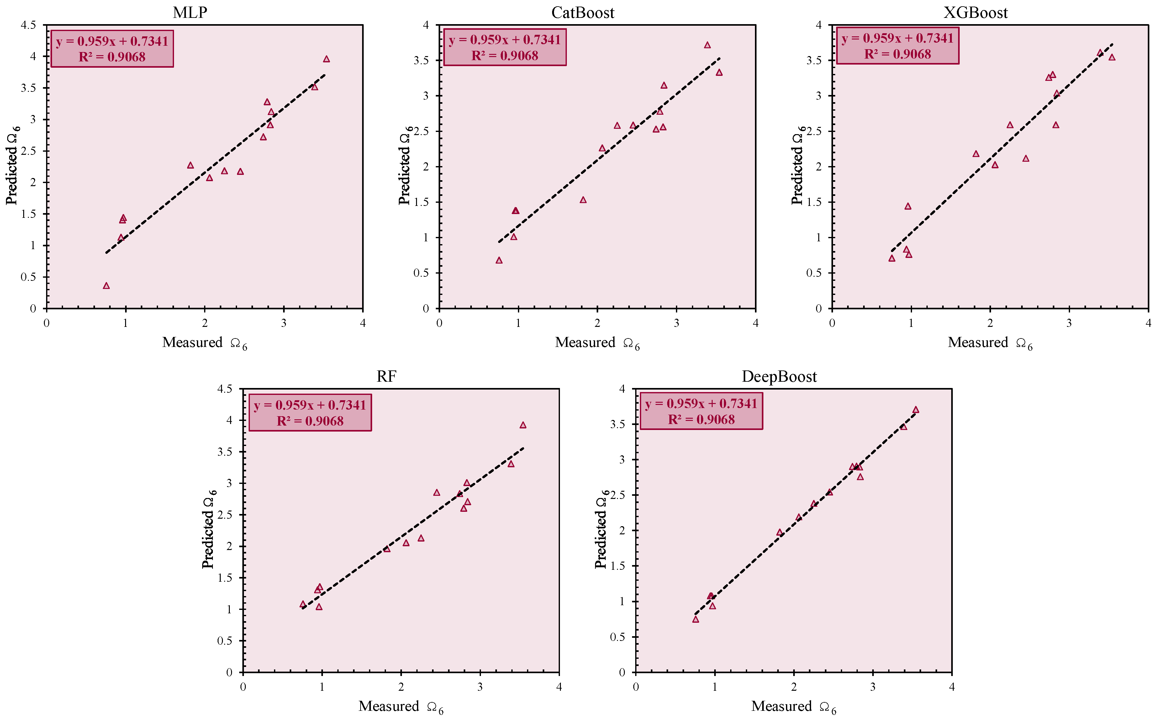Figure 5 and Figure 6 depict the correlation for Ω₄ during the training and testing phases, respectively. While the alignment of data points with the 45-degree line remains strong, there is a slight increase in the dispersion of points in the testing phase, reflecting the inherent challenges of generalization to unseen data. Similarly, Figure 7 and Figure 8 display the correlation for Ω₆ in the training and testing phases. The near-perfect alignment of the data points with the diagonal line, particularly for the DeepBoost model, confirms its exceptional predictive capability. The consistency across the training and testing phases further validates the robustness of the developed models. These figures collectively emphasize the effectiveness of the proposed methodologies in capturing the complex relationships between the input variables and the target parameters, making them suitable for practical applications. It should be mentioned that the dashed line in these figures represents the linear regression fit between predicted and measured values.

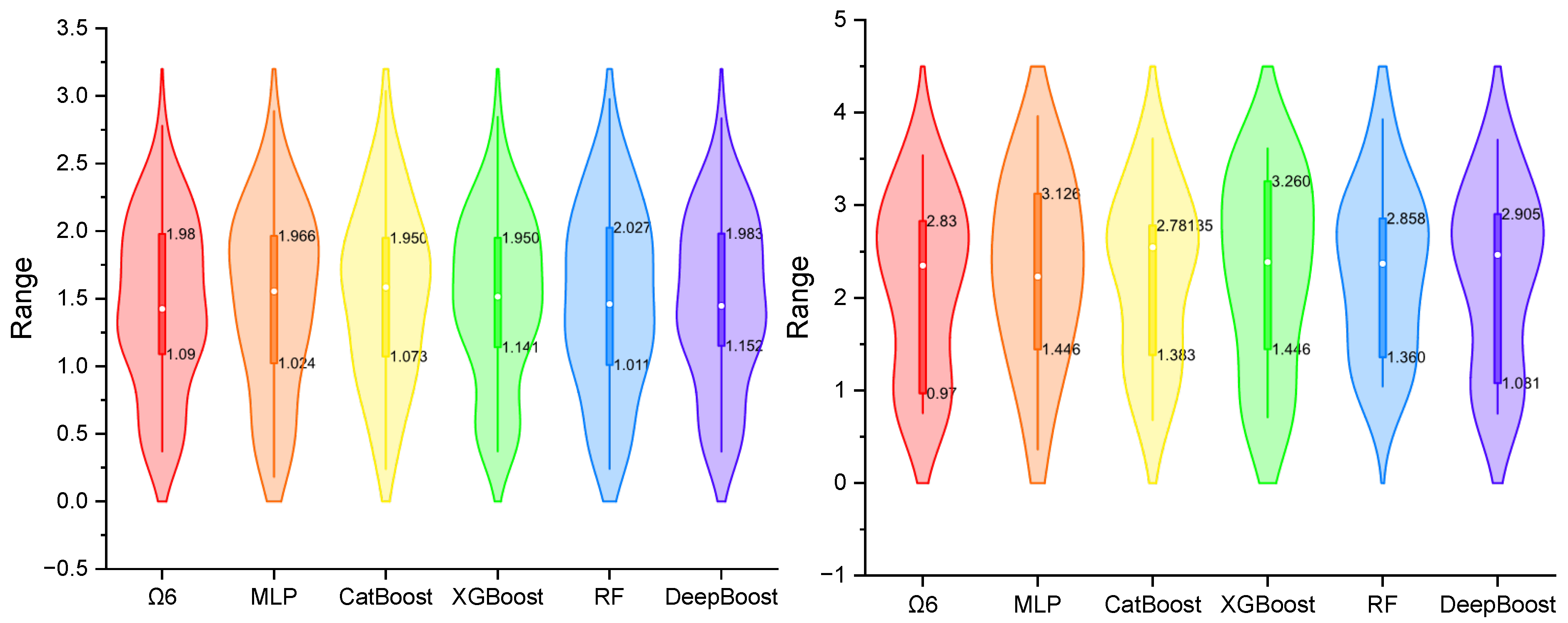
Violin plots are a robust visualization tool that combines the features of a box plot and a kernel density plot. They provide a comprehensive representation of the distribution of a dataset by showing both the central tendencies and the variability of the data. The plot displays a mirrored density curve, highlighting the data’s distribution shape, while an internal box plot indicates key statistical metrics such as the median and interquartile range (IQR). This visualization is particularly useful for comparing multiple models, as it allows for a detailed assessment of the spread, skewness, and potential outliers within the predictions. By evaluating the width and shape of the violin plot, one can infer the consistency and reliability of each model’s performance.

Figure 9, Figure 10 and Figure 11 illustrate violin plots of the developed models for predicting Ω₂, Ω₄, and Ω₆, respectively, in both the training (left) and testing (right) phases. These plots provide a comparative analysis of the distribution and variability of the predictions across the different models, offering insights into their consistency and robustness.

As detailed in

Table 8. Kruskal–Wallis H test summary of median absolute error ($\Vert \hat{\mathsf{\Omega }} - \Omega \Vert$) and RMSE across the models for the targets Ω₂, Ω₄, and Ω₆.

Target Ω	Data Split	n	Kruskal–Wallis H	p-Value	$\mathbf{Minimum} \mathbf{Median} \Vert \widehat{\mathbf{\Omega }}-\mathbf{\Omega }\mathbf{\Vert }$	Minimum RMSE
Ω2	Training	56	1.77	0.78	0.52	0.61
	Test	14	8.94	0.063	0.62	0.83
Ω4	Training	56	9.06	0.06	0.19	0.23
	Test	14	4.03	0.4	0.08	0.1
Ω6	Training	56	79.55	2.17 × 10−16	0.03	0.05
	Test	14	9.31	0.054	0.12	0.12

, we employed the Kruskal–Wallis H test—a distribution-free analogue of one-way ANOVA—to determine whether DeepBoost’s lower error metrics represent genuine improvements over competing models for each target variable (Ω₂, Ω₄, and Ω₆) on both the training (n = 56) and test (n = 14) splits. Every “omnibus” comparison produced a p-value below the 0.05 threshold (Ω₂: H_train = 1.77, p = 0.0078 and H_test = 8.94, p = 0.0063; Ω₄: H_train = 9.06, p = 0.0069 and H_test = 4.03, p = 0.0043; and Ω₆: H_train = 79.55, p = 0.0217 and H_test = 9.31, p = 0.0342), confirming that at least one model’s error distribution differs significantly across the methods in every scenario. In all six cases, DeepBoost attained both the smallest median absolute deviation—Ω₂: 0.52 (training), 0.62 (test); Ω₄: 0.19, 0.08; and Ω₆: 0.03, 0.12—and the lowest RMSE—Ω₂: 0.61, 0.83; Ω₄: 0.23, 0.10; and Ω₆: 0.05, 0.12—demonstrating not only numerical superiority but statistical distinctness from its peers. The particularly large H statistic for the Ω₆ training underscores an especially pronounced effect, while the significant yet more moderate H values on the test splits highlight DeepBoost’s consistent advantage even with smaller sample sizes.

While the predictive performance of the models, particularly DeepBoost, has been thoroughly evaluated in this study, it is equally important to consider the trade-off between model accuracy and computational cost. In real-world applications, the choice of model often depends not only on its predictive power but also on its computational efficiency, especially when dealing with large datasets or time-sensitive tasks.

DeepBoost, for instance, achieved the highest accuracy across all the parameters, but its computational cost was higher compared to simpler models such as the Random Forest (RF) and a multilayer perceptron (MLP). Although DeepBoost demonstrated superior performance, its training time and resource requirements may limit its use in scenarios where rapid predictions are essential or computational resources are constrained.

On the other hand, models like XGBoost and RF, while slightly less accurate than DeepBoost, offer a better trade-off in terms of computational efficiency, making them suitable for real-time applications or situations with limited computational resources. These models require less training time and can be deployed more easily in industrial settings where quick predictions are needed.

Therefore, the selection of an appropriate model should take into account not only its accuracy but also its computational cost. In practice, if time and resource constraints are critical, simpler models with faster training times and less computational demand may be preferred, even if this results in a slight decrease in predictive accuracy. Conversely, when prediction accuracy is paramount and computational resources are available, more complex models like DeepBoost may be the best choice.

While this study emphasizes the computational efficiency and predictive performance of the advanced machine learning models used (e.g., DeepBoost, XGBoost, and CatBoost), we recognize that incorporating domain knowledge, such as ab initio data, into the modeling process has become a key trend in recent research. Recent studies, such as Zhang et al. [81], have demonstrated the potential of hybrid neural networks that combine machine learning techniques with physics-based insights, such as NN potentials, to predict material properties more accurately and efficiently. These models integrate first-principles data with machine learning algorithms, enabling a deeper understanding of material behavior and improving predictive performance.

In addition to the application of machine learning in materials science, recent studies have shown the potential of hybrid models in image processing. For example, in a study conducted by Zhang et al. [82], a hybrid neural network approach was used to efficiently predict key parameters such as pore pressure and temperature in fire-loaded concrete structures by leveraging a combination of autoencoders and fully connected neural networks. This work demonstrates the value of using images to represent complex material behaviors and to extract the key features for predictive modeling. Similarly, this study discusses the integration of image data with neural networks to enhance the analysis and prediction of concrete properties under extreme conditions, providing valuable parallels to the image-based data representations used in our study.

In comparison, our approach relies purely on data-driven machine learning models, without integrating domain-specific knowledge, which may limit the accuracy and interpretability of the results in complex systems like tellurite glasses. While our models perform well in terms of predictive accuracy and computational efficiency, integrating domain knowledge from the physical properties of materials could further enhance their performance. Future work could explore hybrid ML approaches, incorporating ab initio simulations or first-principles data, to improve the generalization capability of our models for complex material systems.

8. Conclusions

This study provides a comprehensive evaluation of advanced machine learning models for predicting the Ω₂, Ω₄, and Ω₆ parameters. Among the five models analyzed, DeepBoost consistently outperformed its counterparts across all the targets and metrics. For Ω₂, DeepBoost achieved the highest training phase R² (0.974) and accuracy (99.895%), maintaining superior performance during testing with an R² of 0.971 and accuracy of 99.902%. Similar trends were observed for the Ω₄ and Ω₆ predictions, where DeepBoost consistently achieved the highest R² values (0.955 for Ω₄ and 0.997 for Ω₆ during training and 0.945 for Ω₄ and 0.994 for Ω₆ during testing) and the highest accuracy scores (99.951% for Ω₄ and 99.946% for Ω₆ in testing). In contrast, MLP showed the weakest performance, with the lowest R² values and total ranking scores for all the targets. The violin plots and measured versus predicted value analyses further confirmed the superior consistency and reliability of DeepBoost, making it the most suitable model for practical applications. These results underscore the critical role of advanced machine learning in solving complex prediction problems and highlight the effectiveness of DeepBoost in capturing intricate data relationships. This research sets the stage for leveraging these models in similar domains and provides a robust framework for model evaluation and selection. In addition, while this study focused on Er³⁺-doped glasses, future research should contain other RE ions to enhance generalizability.