Advancing CVD Risk Prediction with Transformer Architectures and Statistical Risk Factor Filtering

Abstract

Cardiovascular disease (CVD) remains one of the leading causes of mortality worldwide, demanding accurate and timely prediction methods. Recent advancements in artificial intelligence have shown promise in enhancing clinical decision-making for CVD diagnosis. However, many existing models fail to distinguish between statistically significant and redundant risk factors, resulting in reduced interpretability and potential overfitting. This research addresses the need for a clinically meaningful and computationally efficient prediction model. The study utilizes three real-world datasets comprising demographic, clinical, and lifestyle-based risk factors relevant to CVD. A novel methodology is proposed, integrating the HEART framework for statistical feature optimization with a Transformer-based deep learning model for classification. The HEART framework employs correlation-based filtering, Akaike information criterion (AIC), and statistical significance testing to refine feature subsets. The novelty lies in combining statistical risk factor filtration with attention-driven learning, enhancing both model performance and interpretability. The proposed model is evaluated using key metrics, including accuracy, precision, recall, F1-score, AUC, and Jaccard index. Experimental results show that the Transformer model significantly outperforms baseline models, achieving 93.1% accuracy and 0.957 AUC, confirming its potential for reliable CVD prediction.

1. Introduction

Cardiovascular diseases (CVDs) are still the leading cause of death worldwide, with an estimated 17.9 million deaths per year, accounting for 32% of all global deaths, according to a report by the World Health Organization [1] in 2023. Of these, 85% relate to heart attack and stroke, highlighting the crucial reliance on implementing early and accurate risk prediction. Although there are numerous ML methods that assess CVD risk, most of them treat all risk factors equally, which also includes statistically insignificant features; consequently, they may experience overfitting, unnecessary diagnosis costs, and decreased clinical interpretability [2,3]. Additionally, classic ML algorithms like random forests, SVMs, and ensemble methods have only demonstrated a rudimentary ability to capture complex nonlinear associations and feature dependencies that are relevant to CVD prediction tasks [4].

In light of these challenges, we present a Transformer-based framework for cardiovascular disease prediction, as the self-attention mechanism enables dynamic weighting of risk factors conditioned on their context. Whereas previously published work has shown promise with different ensemble neural models, particularly stacked meta neural networks (SMNNs) [5], in this work, we push the boundaries of the state of the art further by leveraging the transition between architectures and statistically filtered risk factors as implemented via a hybrid feature selection pipeline that combines correlation-based filtering followed by Akaike information criterion (AIC) and significance-based risk factor reduction. We utilize attention visualization, which reflects the feature importance, thus providing not only model accuracy but also ensuring understanding of the model predictions.

It is in the combination of explainable deep learning and statistically optimized input dimensions that this work is novel, producing a clinically relevant and computationally efficient model. This paper contributes to the literature scientifically by (i) showing that Transformers outperform the most used ML techniques and hybrid ensemble classifiers in CVD tasks; (ii) proposing an interpretable and cost-effective diagnostic pipeline; and (iii) validating our approach with several benchmark datasets and k-fold cross-validation while being more robust and higher in accuracy or AUC than previously proposed models.

With advancements in machine learning and the exponential growth of clinically relevant data, the need for interpretable and efficient predictive systems in healthcare has never been greater, especially in the area of clinical decision support systems (CDSSs), where transparency and trust are vital. Despite their accuracy, traditional black-box models are not always explainable and are, therefore, not suitable for real-time clinical integration [6]. The attention-based mechanism of the Transformer model gives high predictive performance while also helping visualize attention weights, which aids a clinical understanding of factors influencing individual risk prediction [7]. Framing this in light of the balance between performance and interpretability, the hybridization of domain-aware statistical filtering combined with the representational power of Transformers provides a sensible bridge.

Moreover, CVD datasets are usually heterogeneous and unbalanced, including continuous, categorical, and binary features. The use of the HEART framework’s feature selection pipeline—rooted in statistical techniques for assessing distributions of data fit (e.g., Shapiro–Wilk test), correlation types (point-biserial, Cramer’s V, tetrachoric), and model evaluation based on AIC—will guarantee only the most salient, non-redundant features are retained in the proposed study. This statistical rigor minimizes computational burden with minimal loss of clinical relevance. The other part of the proposed framework utilizes outlier removal techniques based on the distribution of data (for example, interquartile range (IQR) and 3σ-based thresholds) that enhance the robustness of the model [2].

In this research, we propose a complete generalization of the existing CVD prediction pipeline based on SMNN to a Transformer-based deep learning model trained on statistically best-performing features. We will evaluate the performance of the proposed model using standard performance metrics such as accuracy, precision, recall, AUC, and F1-score (k-fold cross-validation) on resolved and benchmark datasets like IEEE DataPort Heart Disease, Faisalabad dataset, and South African Heart Disease datasets. Showcasing the enhanced prediction, explainability, and efficiency of our approach compared against existing ensemble and classical ML classifiers. 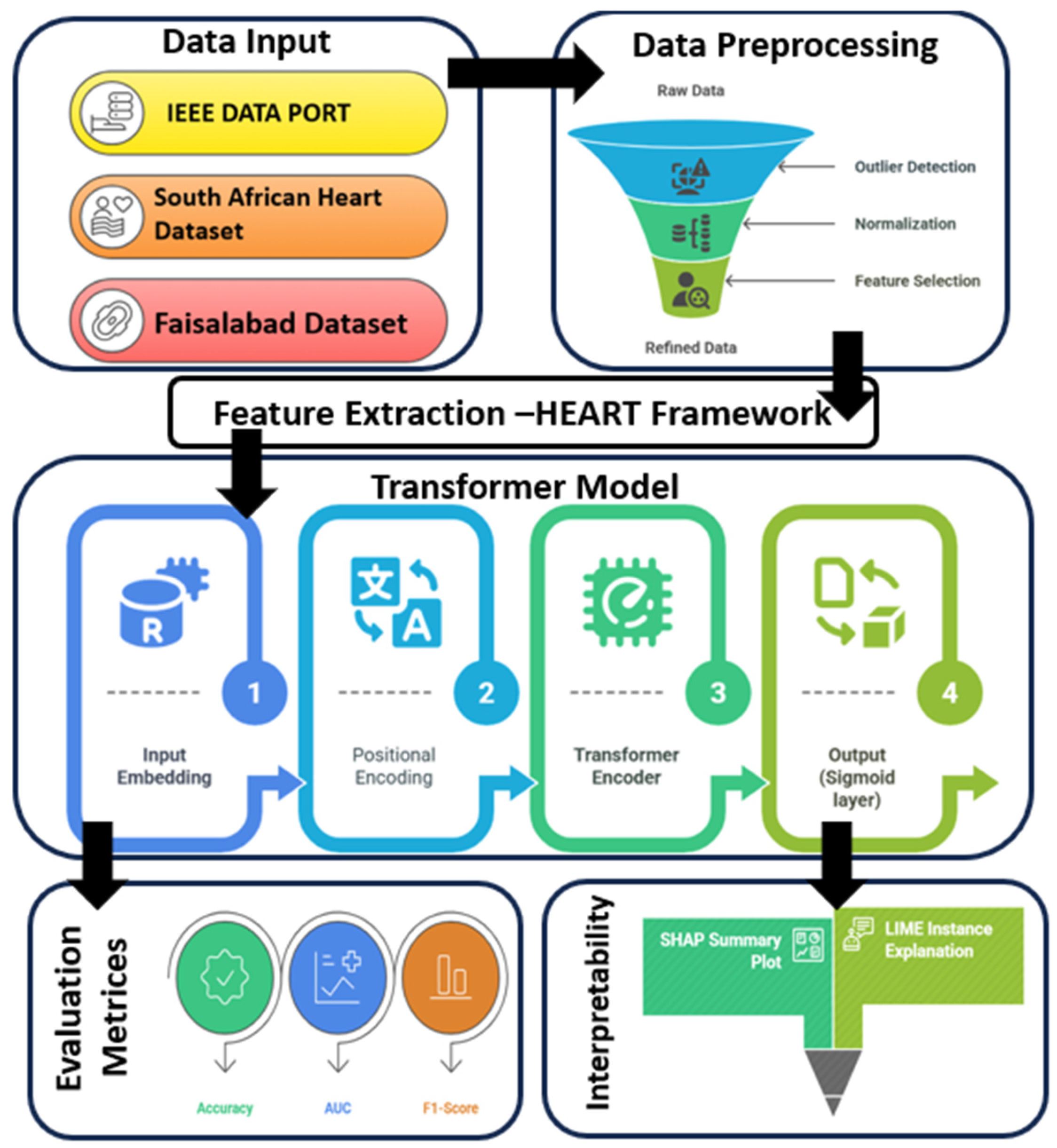Figure 1 represents the workflow of the cardiovascular disease prediction process. This work, therefore, makes significant contributions to the ongoing discourse on CVD prediction by the following:

• Introducing an interpretable, attention-based Transformer model tailored for CVD risk classification;
• Enhancing feature selection rigor through the HEART methodology;
• Improving prediction accuracy and robustness on real-world clinical datasets;
• Reducing the diagnostic burden by eliminating redundant tests and focusing on statistically significant risk indicators.

2. Literature Review

An enormous number of studies using statistical, machine learning (ML), and deep learning (DL) methods for the prediction of cardiovascular disease (CVD) have emerged from the field. The development of accurate early prediction models is crucial to mitigate mortality and improve outcomes in patients. Conventional methods have concentrated on generating risk factors by comparing age, high blood pressure, diabetes, cholesterol levels, and smoking [1,7].

Statistical Approaches: Traditional approaches utilized statistical significance testing and correlation analysis to identify associations between CVD and its risk factors. Researchers [8] employed Pearson correlation on data gathered from hospitals in Saudi Arabia and discovered that hypertension, diabetes, and hyperlipidemia have significant correlations with CVD. Some researchers [9] performed statistical analysis using chi-square and Mann–Whitney U tests for comorbid clusters, including smoking and diabetes, demonstrating their multiplicative effects. While informative, these approaches often fail to capture the complex interdependencies between risk factors and are limited in their application to predictive modeling.

Feature Selection Techniques: Multiple studies have proposed ML-based feature selection algorithms to characterize the significant risk factors. The researchers in [10] compared different selection methods, including ANOVA, mutual information, Relief, and Lasso regression, on the UCI Heart Disease dataset. A method proposed by Theerthagiri and Vidya for the selection of an optimal feature subset is the recursive feature elimination with gradient boosting (RFE-GB) [11]. Nonetheless, these methods often overlook the structure of the data distribution and can preserve features that are redundant or non-beneficial, thus hindering model interpretability and efficiency.

Classification Models: A large variety of classifiers based on machine learning have been used for the prediction of CVD. Extensive use has been made of models like support vector machine (SVM), random forest (RF), decision tree (DT), logistic regression (LR), and Naive Bayes. Another study [12] utilized kernel-based SVM, while E. Sakyi-Yeboah et al. [13] applied ensemble methods that combine M5P and random tree algorithms. Deep learning architectures like artificial neural networks (ANNs) and multi-layer perceptrons (MLPs) have also been notably successful in learning nonlinear behavior [14]. However, such models are variants of black-box systems, providing little transparency for the contribution of each of the features.

Hybrid and Ensemble Models: More recently, researchers have investigated ensemble-based hybrid frameworks to enhance predictive accuracy. Researchers [5,15] demonstrated a hybrid ANN model which combined partial and full correlation differences. They [16] also applied various ML classifiers using SMOTE (synthetic minority over-sampling technique) balance to improve model robustness. However, these systems are often restricted by their rigid structure and lack of contextualization for feature significance.

Review of the Base Paper: The foundational work by Bandyopadhyay et al. [2] introduced a novel two-phase framework combining rigorous statistical analysis with a stacked meta neural network (SMNN). The first phase—Heart Disease Assessment and Review Technique (HEART)—integrates correlation-based filtering, Shapiro–Wilk-guided distribution testing, and AIC to identify a minimal, statistically significant set of key risk factors. In the second phase, the SMNN model stacks six ML classifiers (RF, ET, LR, DT, SVM, and KNN), whose outputs are fed into an ANN meta-learner. Their approach yielded average accuracies of 90.5% (IEEE DataPort), 88.5% (Faisalabad dataset), and 80.3% (South African dataset), demonstrating high robustness. However, the SMNN still suffers from limitations in interpretability and generalization of unseen data, particularly given its reliance on ensemble techniques without leveraging dynamic attention mechanisms.

Need for Advancement: The current literature shows substantial advances in CVD prediction but retains some key gaps. The majority of models battle overfitting, non-explainability, and inefficient feature usage. Additionally, the implementation of Transformer-based architectures, which enforce self-attention and efficiently model complex dependencies, is rare. We fill these gaps in this work by incorporating the Transformer model into the pipeline with HEART optimization to further boost accuracy and interpretability while transitioning closer to the clinic.

3. Research Gap and Problem Statement

3.1. Research Gap

Despite the significant advancements in cardiovascular disease prediction using machine learning and hybrid ensemble frameworks, several critical gaps persist in the existing literature:

1.

Lack of Interpretability in Deep Learning Models: Deep neural networks and ensemble classifiers achieve the best prediction accuracy, but many of these models are black boxes, giving little insight into how individual risk factors determine the outcome. This lack of transparency restricts their use in clinical decision-making frameworks, where explainability is particularly important.

2.

Inefficient Handling of Feature Importance: Many existing models, including high-performing ensemble methods, fail to dynamically adjust feature relevance during prediction. Traditional models treat input features with static weights, which may not reflect real-time physiological interactions among risk factors.

3.

Limited Use of Attention-Based Architectures: The capabilities of Transformer-based models have not yet been explored in the literature on CVD prediction. While Transformers have extended the frontiers of the natural language processing and image classification fields by utilizing attention mechanisms for long-range redundancy of information [17], the use of a Transformer framework on clinical tabular data is relatively nascent.

4.

Overreliance on Redundant and Non-significant Features: Most studies use complete-feature datasets without statistical filtering, leading to computational loss and higher diagnostic costs. While the HEART framework attempts to solve this challenge through correlation analysis, AIC, and filtering based on distribution, it does not yet integrate adaptive learning models (such as Transformers).

5.

Static Architecture of Ensemble Models: The base paper uses stacked models for SMNN (stacked meta neural network) [2], which come with a fixed ensemble architecture and are incapable of adapting over a dataset, nor does a feature relationship increase the context of a feature.

3.2. Problem Statement

Cardiovascular diseases are responsible for the largest share of global deaths; hence, timely and precise predictive systems that are efficient and interpretable are warranted. Current predictive models—everything from traditional classifiers to ensemble neural networks—have typically required some trade-off between explainability and accuracy. Although some frameworks like HEART + SMNN have shown enhanced performance with hybrid designs and statistical filtering, they are still built on static architectures and do not implement dynamic feature weighting strategies.

The main issue is that there is no predictive framework that marries statistical feature selection with adaptive, interpretable deep learning that can contextually represent real-time patient data. It becomes essential to design a Transformer-based diagnostic model with an attention mechanism for better classification performance, which provides feature attribution to increase clinical trust toward the model. This study seeks to fill this void by using a Transformer model combined with statistically identified risk factors to create a robust, interpretable, and clinically relevant predictive system for cardiovascular disease.

4. Dataset Description

The proposed Transformer-based cardiovascular disease (CVD) prediction framework was evaluated across different publicly available benchmark datasets to measure its performance and generalizability in this study. These datasets differ in demographic profiles, sample sizes, and feature sets, allowing a thorough evaluation of the proposed model on varied populations.

Table 1. Comparative overview of the datasets used for cardiovascular disease prediction.

Attribute	IEEE DataPort	Faisalabad Dataset	South African Heart Disease Dataset
Source	IEEE DataPort Repository	UCI Repository (Univ. of Faisalabad, Pakistan)	South African Medical Research Council
Region Represented	Global (Mixed Population)	South Asia (Pakistan)	Africa (South Africa)
Total Records (Samples)	918	1025	462
Initial Number of Features	18	14	10
Numerical Features	10	9	6
Categorical Features	5	3	2
Binary Features	3	2	2
Target Variable	CVD Presence (Binary)	Heart Disease (Binary)	Heart Disease (Binary)
Positive Class (CVD Present)	470	540	237
Negative Class (CVD Absent)	448	485	225
Class Balance (Positive/Negative)	51.2%:48.8%	52.7%:47.3%	51.3%:48.7%
Missing Values	No	No	No
Outlier Handling Applied	Yes (IQR and 3σ-based removal)	Yes	Yes
Feature Normalization Applied	Yes (Z-score Standardization)	Yes	Yes
Statistical Feature Selection Method	HEART Framework (Correlation + AIC + Tests)	Same	Same
Final Features Used in Modeling	10	8	6
Dataset #	Dataset 1	Dataset 2	Dataset 3

provides a clear comparison of the three datasets used in the study: IEEE DataPort, Faisalabad Dataset, and South African Heart Disease Dataset, highlighting where they come from, the regions they represent, their sample sizes, their features, how the classes are distributed, the preprocessing methods used, and the final features applied in the proposed Transformer framework.

4.1. IEEE DataPort Heart Disease Dataset

The initial dataset used in this research was obtained from the IEEE DataPort repository [17]. This dataset contains 918 patient records and 18 clinical features, which are both categorical and continuous attributes associated with cardiovascular health. The following are the key features: age, sex, history of smoking, blood pressure, cholesterol, diabetes, and electrocardiogram results. All independent variables were derived from the features, while the dependent variable (target) is binary, confirming whether the participant has CVD or not. The dataset is a balanced and organized dataset viable for supervised classification tasks.

4.2. Faisalabad Heart Patient Dataset

The second dataset can be found in the Heart Disease UCI repository and is contributed by the University of Faisalabad, Pakistan [18]. The dataset contains 1025 instances and 14 feature vectors comprising a mix of demographic and clinical parameters, including type of chest pain, resting blood pressure, serum cholesterol, fasting blood sugar, and maximum heart rate achieved. The objective variable is ENSUM, which identifies if a patient has symptoms of vessel disease. This dataset is relatively clean and complete (with few missing values) and has been used frequently in comparative research on the prediction of heart disease.

4.3. South African Heart Disease Dataset

The third dataset was obtained from the South African Heart Disease Study [19]. The dataset consists of 462 records of patients with 10 different features such as systolic blood pressure, use of tobacco, consumption of alcohol, obesity index, family history of heart disease, etc. This dataset is especially pertinent, as it is focused on lifestyle-related risk factors and a less studied geographic population. It has a binary target variable, where the target variable indicates whether a patient is diagnosed with heart disease or not.

5. Proposed Methodology

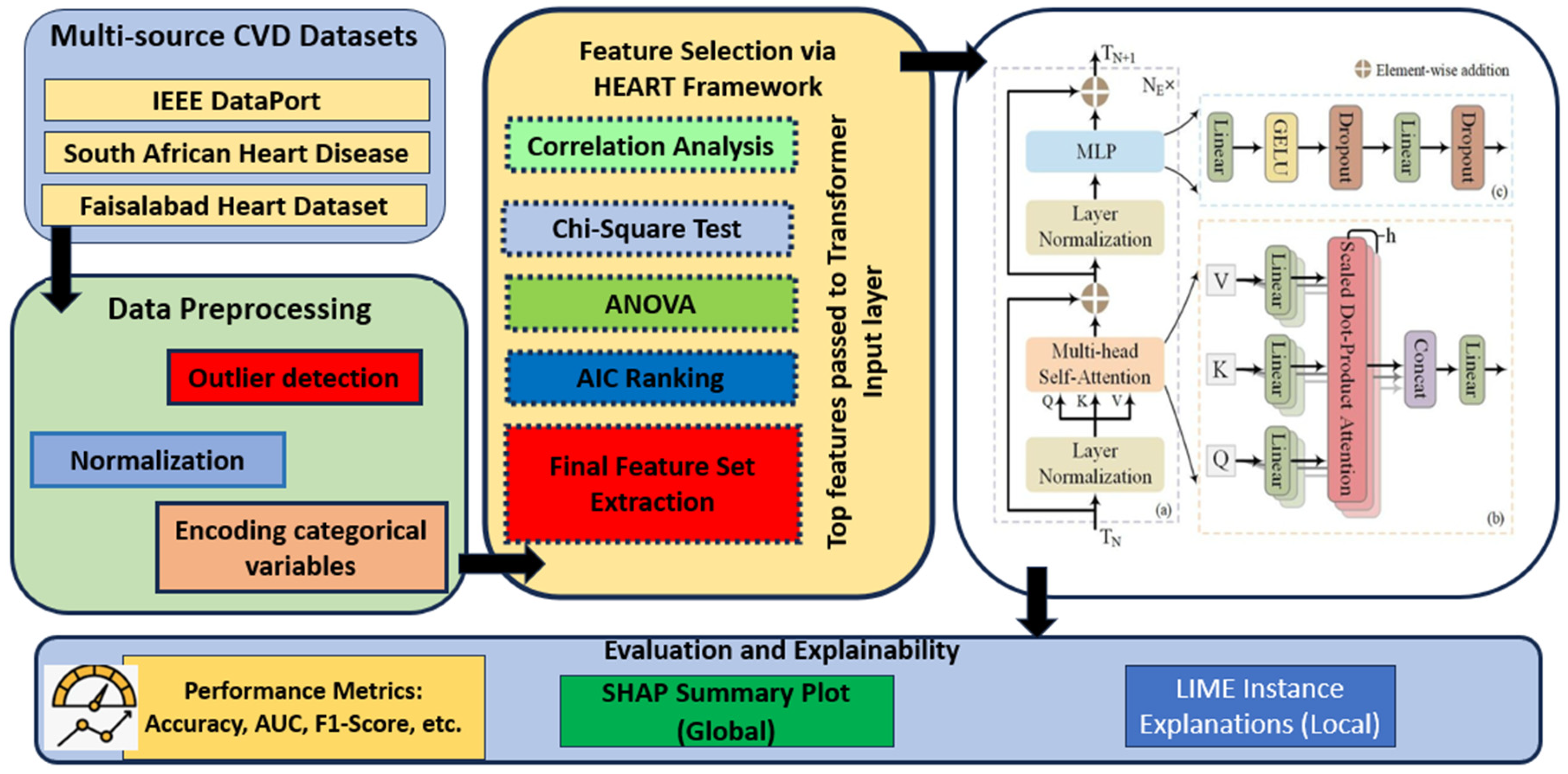
For the sake of clarity, reproducibility, and methodological transparency, this section is organized into six integrated subsections comprising the full model pipeline for CVD risk prognostication. It starts with data gathering and preprocessing steps and proceeds by utilizing the HEART framework for statistical filtration of risk factors. Next, we describe the Transformer architecture used for predictive modeling. The following subsection describes the model training and hyperparameter configurations. This phase is then followed with a brief review of the evaluation metrics used to measure how well bats’ predictions are. Finally, the SHAP-based (Shapley additive explanations) explainability module is given to interpret the model outputs. We conceive these aspects of the methodology to facilitate reproducibility and enhance the scientific soundness of the approach. Figure 2 shows the workflow of the methodology.

5.1. Data Collection and Preprocessing

The study used publicly available datasets, as introduced in Section 1, i.e., patient data with structured clinical and demographic features. The datasets were processed through a common preprocessing pipeline before model construction. The procedure entailed dealing with the missing values via the mean or mode imputation (as appropriate for the attribute). Outliers were detected by IQR analysis and dropped. While categorical features were converted to one-hot representation, numerical inputs were normalized with min–max normalization to guarantee consistent input distributions. The resultant clean datasets were split into training and testing sets in an 80:20 stratified manner (keeping class distributions balanced). This additional step of preprocessing the data was to maintain the quality of data and consistency for subsequent statistical filtering and modeling.

5.2. Statistical Feature Optimization Using the HEART Framework

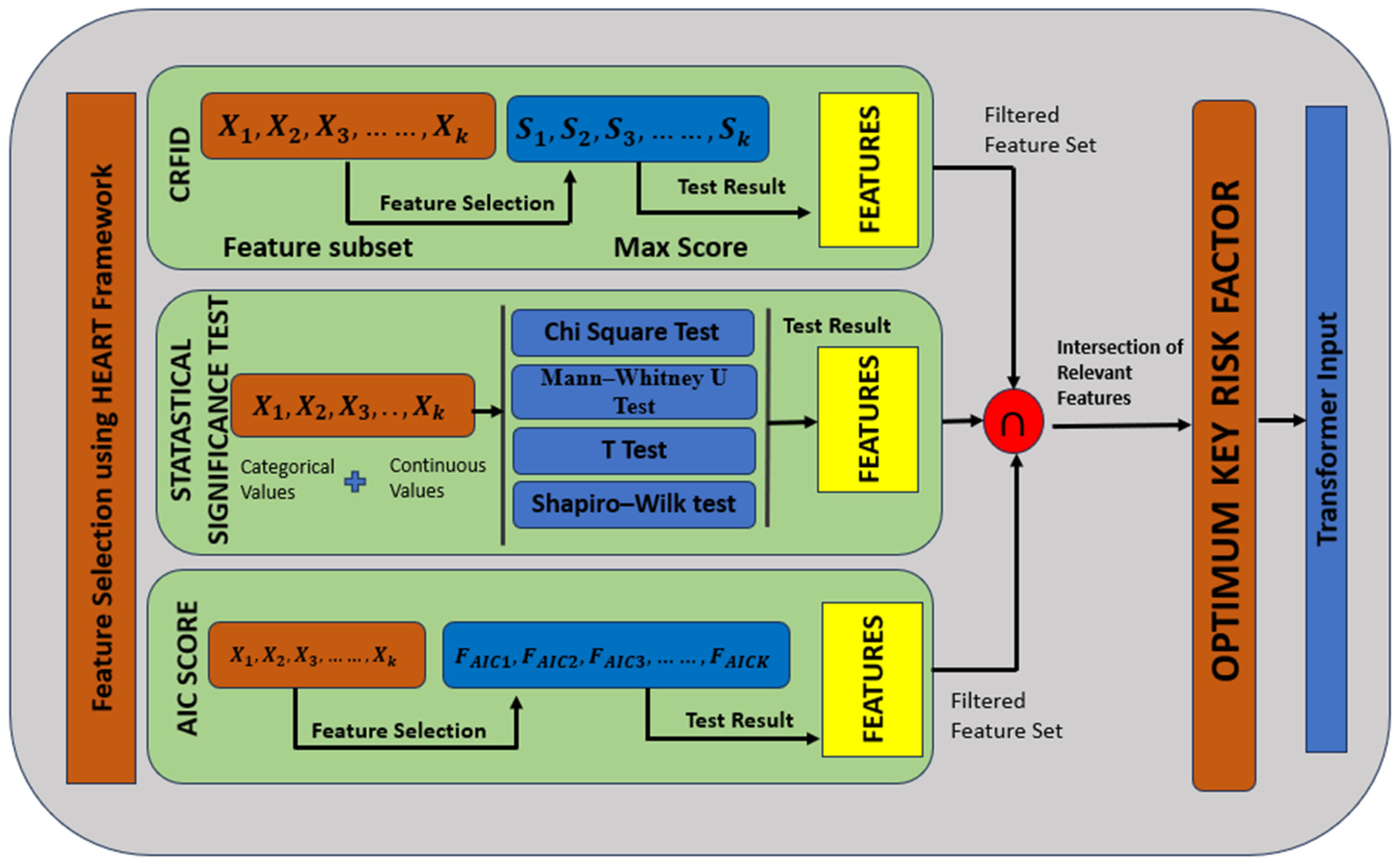
The HEART (Heart Disease Assessment and Review Technique) framework is a structured, mathematically grounded three-phase methodology for identifying optimum key risk factors for cardiovascular disease (CVD) prediction. Its objective is to reduce dimensionality, improve computational efficiency, and ensure the clinical interpretability of the final classifier. Figure 3 shows how CRFID (correlation-based risk factor identification and discrimination) is computed step by step on a range of feature subset sizes.

An important part of the proposed methodology is the identification of relevant CVD risk factors. This study took a hybrid approach that combines both clinical domain expertise with statistical testing. Clinically, an exhaustive list of features was selected in accordance with established guidelines from world cardiovascular authorities, including the World Health Organization and the American Heart Association. Sudden cardiac death during myocardial infarction is an opportunistic event that has been studied extensively, leading to the identification of several features that may predict risk, including demographic variables (e.g., age and gender), physiological measurements (e.g., resting blood pressure, cholesterol levels, and maximum heart rate), behavioral factors (e.g., smoking and alcohol consumption), medical history (e.g., diabetes, prior cardiac events, and family history), and electrocardiographic indicators (e.g., ST depression and chest pain type). However, for model training, a strict statistical filtering process was implemented using HEART (Heart Disease Assessment and Review Technique), which ensured only the most relevant, non-redundant variables were leveraged.

This framework is based on three phases: (1) correlation-based filtering (to assess whether a direct association with CVD exists), (2) distribution-based testing (to assess normality and outlier detection), and (3) a model-based feature selection (using AIC) to retain only those variables that materially improve model fit). From the variable selection process, the final set of factors for oncology was determined to be those that completed statistical checking (the three phases of statistical tests) as well as clinical biologist analysis. In all three benchmark datasets—IEEE DataPort, Faisalabad, and South African—the features, including age, resting blood pressure, cholesterol level, max heart rate achieved, ST depression, diabetes, and smoking status, were consistently selected as optimum key predictors. These risk factors serve as the basis for the Transformer-based prediction model used in this study. The C-RFID framework computes a score for selecting the optimal subsets of risk factors, balancing correlation to the target (i.e., relevance) and collinearity among features (i.e., inter-correlation) in the risk factor set.

The phases are the following: (i) Correlation-Based Filtering, (ii) Distribution and Outlier Analysis, and (iii) Model-Based Selection using the AIC. Figure 4 shows the HEART workflow.

5.2.1. Phase I: Correlation-Based Filtering

This phase quantifies the statistical association between each feature Xj and the binary response variable Y ∈ {0,1} (absence or presence of CVD). The choice of correlation metric depends on the data types involved. Some of the statistical formulations we use in our model—such as the Point-Biserial correlation, Cramer’s V coefficient, and AIC—have been drawn from the literature, especially from the seminal work by Bandyopadhyay et al. [2]. The stacked ensemble approach with k-fold cross-validation and base/meta learner feature transformations is also borrowed from this work. We acknowledge the direct reuse of these techniques for the purpose of consistency, benchmarking, and comparison.

The Pearson correlation coefficient (continuous–continuous) can be represented by Equation (1).

$${\rho }_{xy}={\displaystyle \frac{\sum _{i=1}^n(x_i-\overline{x})(y_i-\overline{y})}{\sqrt{\sum _{i=1}^n{(x_i-\overline{x})}^2. }\sqrt{\sum _{i=1}^n{(y_i-\overline{y})}^2}}}$$

(1)

Features are retained if ∣ρ_xy∣ ≥ τ|, where τ is a correlation threshold (commonly 0.1).

Point-Biserial correlation (continuous–binary) can be calculated by Equation (2):

$$r_{pb}={\displaystyle \frac{{\overline{X}}_{1 }-{\overline{X}}_{0 }}{s_X}}. \sqrt{{\displaystyle \frac{n_1{n}_0}{n(n-1)}}}$$

(2)

where:

• ${\overline{X}}_{1 }, {\overline{X}}_{0 }$ are mean values of X for Y = 1 and Y = 0;
• $s_X$ is the standard deviation of X;
• $n_1{n}_0$: class sample sizes.

Cramer’s V (categorical–categorical) can be calculated by Equation (3)

$$V=\sqrt{{\displaystyle \frac{\frac{{\chi }^2}{n}}{\mathrm{m}\mathrm{i}\mathrm{n} (k-1,r-1)}}}$$

(3)

where:

• χ²: Pearson chi-square statistic;
• n: total samples;
• k, r: number of levels in the row and column variables.

Tetrachoric correlation (binary–binary) is used when both variables are binary but assumed to arise from underlying continuous normal distributions. Only features with strong and statistically significant correlation values are passed to the next phase.

5.2.2. Phase II: Distribution and Outlier Analysis

The second phase evaluates whether features follow a normal distribution and detects outliers to ensure robustness.

(a)

The Shapiro–Wilk test for normality can be calculated by Equation (4):

$$W={\displaystyle \frac{{\left(\sum _{i=1}^n{a}_i{x}_{\left(i\right)}\right)}^2}{\sum _{i=1}^n{(x_i-\overline{x})}^2}}$$

(4)

where:

x_(i):

ith order statistic;

a_i:

constants based on the covariance matrix of expected order statistics.

A feature is considered non-normally distributed if the test returns p < 0.05.

(b)

Outlier Detection

Two different methods are used based on the distribution:

i. The Z-score Method (for normal distributions) can be calculated by Equation (5):

$$z_i={\displaystyle \frac{x_i-\mu }{\sigma }}$$

(5)

A sample ${\mathit{x}}_{\mathit{i}}$ is considered an outlier if ∣${\mathit{z}}_{\mathit{i}}$∣ > 3.

ii. IQR Method (for non-normal distributions) can be calculated by Equation (6):

$$\begin{gathered} IQR=Q3-Q1 \\ \mathrm{Outlier} \mathrm{if} x<Q1-1.5·IQR or x>Q3+1.5·IQR \end{gathered}$$

(6)

Features heavily contaminated with outliers or a skewed distribution may be transformed (e.g., log-scaling) or discarded.

5.2.3. Phase III: Model-Based Feature Selection Using AIC

In this phase, logistic regression models are iteratively fitted using combinations of retained features, and the AIC is used to determine the most parsimonious subset.

The Logistic Regression Model uses Equation (7) as follows:

$$P\left(Y=1\left|X\right.\right)={\displaystyle \frac{1}{1+e^{-(}{\beta }_0+{\beta }_1{X}_1+{\beta }_2{X}_2+\cdots +{\beta }_k{X}_k}}$$

(7)

AIC is computed with Equation (8), as in base paper [2]:

$$AIC=2k-2\mathit{ln}(\widehat{L})$$

(8)

where:

k: number of model parameters (including intercept);

$\widehat{L}$: maximum likelihood of the model.

A forward/backward selection strategy is used as follows:

Forward AIC Selection: Start with the null model and add features that reduce AIC.

Backward AIC Elimination: Start with the full model and remove features that increase AIC.

The final selected feature set minimizes AIC and improves the likelihood of predicting the response variable Y.

5.2.4. Output of the HEART Framework

At the end of the HEART pipeline, the dataset X ∈ R^n×p is transformed into a reduced form X′ ∈ R^n×p′, where p′ < p, retaining only the optimum key risk factors given by Equation (9).

X′ = {X_j∣j∈S},

(9)

where S is the optimal feature subset selected via HEART.

These features are then input to the Transformer-based classifier, ensuring the overall model is:

• Statistically sound;
• Computationally efficient;
• Clinically interpretable.

5.3. Transformer-Based Classification Model

Following the statistical optimization of features using the HEART framework, a Transformer-based classification model is employed to predict cardiovascular disease (CVD) outcomes [20,21,22,23]. Transformers, initially designed for unstructured data, have been adapted for tabular data to leverage their ability to model complex relationships between features [24,25]. The FT-Transformer (FTT) customizes the Transformer model for tabular data, showing high performance by considering relationships between all features through the attention mechanism [20]. Unlike traditional machine learning classifiers or static neural networks, the Transformer allows the model to weigh the relative importance of each feature contextually across patients, thus enhancing both predictive performance and interpretability [26,27]. 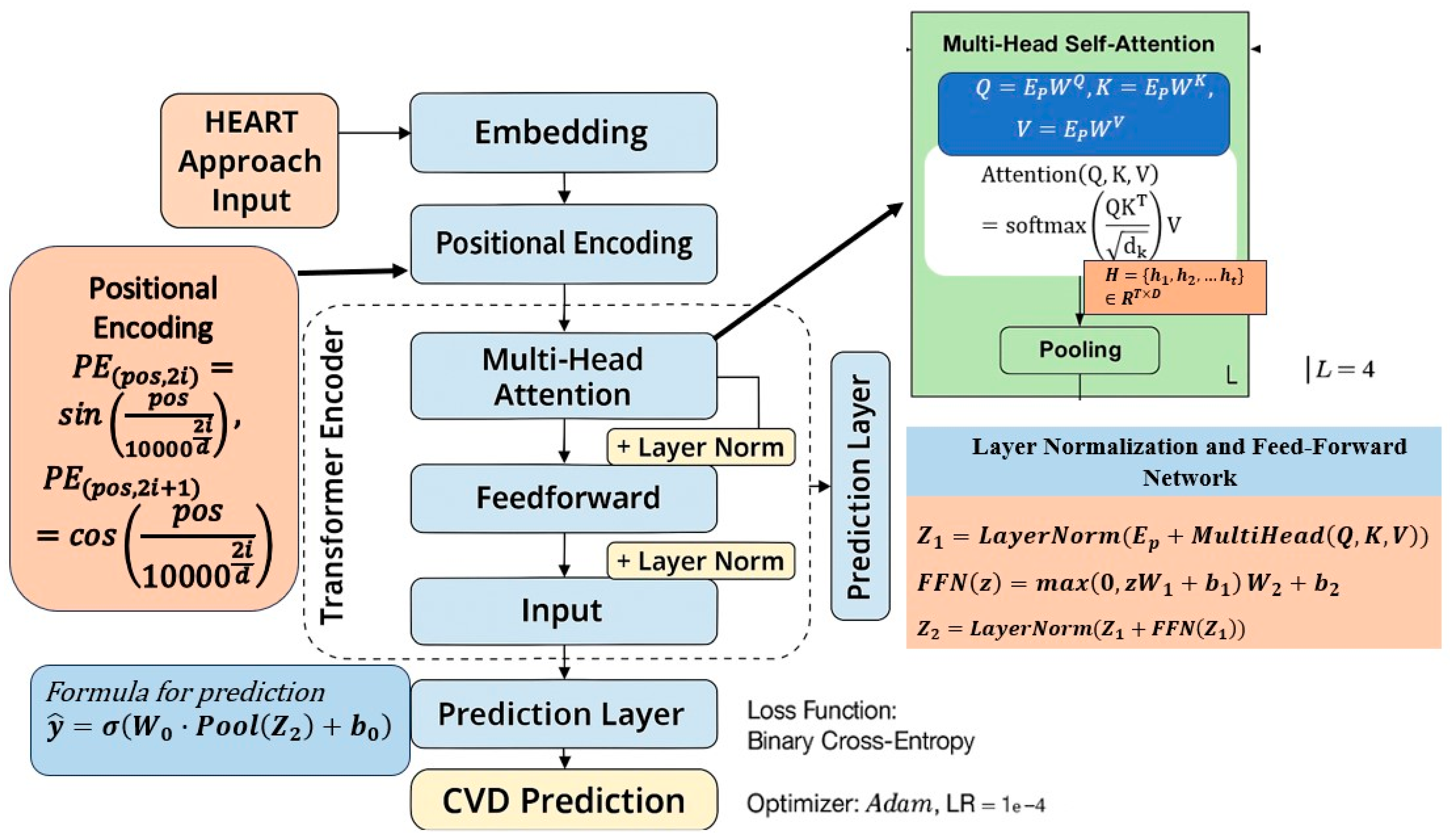Figure 5 shows the detailed architecture of the Transformer-based classification model.

5.3.1. Input Transformation and Embedding

The optimized feature set X′ ∈ R^n×p′, where n is the number of samples and p′ is the number of statistically selected features, serves as the input [28]. Each categorical variable x_i is transformed into a dense vector representation using an embedding layer, as in Equation (10).

e_i = Embed(x_i) ∈ R^d

(10)

where d is the embedding dimension. For numerical features, a linear transformation is applied, as per Equation (11).

h_i = W_nx_i + b_n

(11)

resulting in a unified feature representation space. The embedded input matrix E ∈ Rp′ × d then undergoes positional encoding, ensuring that positional distinctions between features are preserved—even in tabular data.

5.3.2. Positional Encoding

Although feature order is not naturally sequential in tabular datasets, positional encodings are introduced to allow the model to distinguish between input dimensions [29]. The sinusoidal positional encoding function is defined as in Equation (12). The final input embedding becomes Ep, as given in Equation (13).

$${PE}_{(\mathrm{p}\mathrm{o}\mathrm{s},2\mathrm{i})}=\sin \left({\displaystyle \frac{pos}{{\mathrm{10,000}}^{\frac{2i}{d}}}}\right),{PE}_{(\mathrm{p}\mathrm{o}\mathrm{s},2\mathrm{i}+1)}=\cos \left({\displaystyle \frac{pos}{{\mathrm{10,000}}^{\frac{2i}{d}}}}\right),$$

(12)

Ep = E + PE

(13)

5.3.3. Multi-Head Self-Attention Mechanism

The core of the Transformer is the multi-head self-attention mechanism, which computes how each feature attends to others. This is shown in Equation (14).

$$\mathrm{A}\mathrm{t}\mathrm{t}\mathrm{e}\mathrm{n}\mathrm{t}\mathrm{i}\mathrm{o}\mathrm{n}(\mathrm{Q},\mathrm{K},\mathrm{V})=\mathrm{s}\mathrm{o}\mathrm{f}\mathrm{t}\mathrm{m}\mathrm{a}\mathrm{x}\left({\displaystyle \frac{Q{K}^T}{\sqrt{d_k}}}\right)V$$

(14)

where the query (Q), key (K), and value (V) matrices are obtained via Equation (15):

$$Q=E_P{W}^Q,K=E_P{W}^K,V=E_P{W}^V$$

(15)

This operation is performed over multiple heads and can be represented by Equation (16).

$$MultiHead(Q,K,V)=Concat({head}_{1,}\dots \dots ,{head}_h)W^O$$

(16)

Each head enables the model to learn from different subspaces of the feature representation, thereby enhancing its capacity to model complex dependencies [30].

5.3.4. Layer Normalization and Feed-Forward Network

The attention output is passed through a residual connection and layer normalization, as per Equation (17):

$$Z_1=LayerNorm(E_p+MultiHead\left(Q,K,V\right))$$

(17)

This is followed by a position-wise feed-forward network, as given in Equation (18).

$$FFN\left(z\right)=\mathit{max}\left(0,z{W}_1+b_1\right)W_2+b_2$$

(18)

The final output of the encoder block is given by Equation (19).

$$Z_2=LayerNorm(Z_1+FFN\left(Z_1\right))$$

(19)

In this study, the model comprises two Transformer encoder blocks, each with four attention heads, a dropout rate of 0.2, and a feed-forward dimension of 64.

5.3.5. Output Layer and Prediction

The output from the final encoder layer is aggregated using average pooling and passed through a fully connected layer with a sigmoid activation function as per Equation (20).

$$\widehat{y}=\sigma (W_0·Pool\left(Z_2\right)+b_0)$$

(20)

where $\widehat{y}$ ∈ [0,1] represents the predicted probability of CVD presence.

5.3.6. Loss Function and Optimization

The model is trained using the binary cross-entropy loss function, defined as in Equation (21).

$$L=-{\displaystyle \frac{1}{N}}\sum _{i=1}^N[y_i\mathit{log}\left({\widehat{y}}_i\right)+\left(1-y_i\right)log(1-{\widehat{y}}_i\left)\right]$$

(21)

where $y_i$∈ {0,1} is the ground truth label, and ${\widehat{y}}_i$ is the predicted probability. The model is optimized using the Adam optimizer with a learning rate of 0.001, batch size of 32, and early stopping based on validation AUC to avoid overfitting.

Table 2. Transformer model configuration for CVD prediction.

Component	Specification
Input Dimension	Number of selected features (from HEART)
Embedding Dimension	32
Number of Encoder Layers	2
Attention Heads	4
FFN Hidden Dimension	64
Dropout Rate	0.2
Optimizer	Adam
Epochs	100
Loss Function	Binary Cross-Entropy
Activation	Sigmoid

shows the configuration that defines the architecture and training strategy of the proposed Transformer model used for cardiovascular disease prediction in the study.

This Transformer-based classifier, trained on statistically filtered features from the HEART framework, provides an effective mechanism for high-accuracy CVD prediction. Its interpretability (via attention weights), robustness (via feature filtering), and performance (via deep contextual learning) mark a significant advancement over classical ensemble-based and shallow models.

5.4. Evaluation Metrics

Due to the binary classification problem, the following standard metrics were used: accuracy, precision, recall (sensitivity), specificity, F1 score, and area under the curve (AUC) of the receiver operating characteristic (ROC) curve. These performance measures provide the global performance of the model on both balanced and imbalanced datasets [31,32]. Furthermore, confusion matrices were constructed to view true positives, false positives, true negatives, and false negatives, allowing detailed examination of classification results.

In feature selection, less important or weakly influential features were necessarily considered to impose a negative contribution and systematically removed. In particular, features were ranked with mutual information, ANOVA, chi-square, and AIC, and those below a set of relevancy cutoffs were removed. Both of these features were excluded from the training set and controlled for during SHAP analysis to verify their maintenance at a minimal impact. Although the model is not based on the explicit construction of region–text pairs (unlike in vision-language tasks), the intuition of suppressing irrelevant associations is similar. This makes sure that the model learns from clinically interesting predictors and leads to more predictive power as well as explainability.

Finally, a SHAP-based explainability module was designed to interpret the model predictions and obtain insights into the contribution of individual features to CVD risk classification. SHAP provides an importance score for each feature of a given prediction by quantifying the marginal contribution in a game–theoretic framework. DeepSHAP was employed for this study, which is applicable to deep learning frameworks like Transformers. SHAP values were calculated on the test set for correctly classified and misclassified instances to determine the most important clinical factors. Plots summarizing feature importance and facilitating clinical interpretation of model behavior are represented in bar graph format. This inference layer promotes the transparency of the predictive model and increases the potential application to real-world medical decision-making.

While the Transformer architectures provide an attention mechanism as a basis for providing some explanation, weights of attention alone cannot explain the whole feature-level contribution, particularly in healthcare scenarios requiring trust, traceability, and clinical validation. Therefore, we could use SHAP, which follows a complementary and model-agnostic approach to quantify the contribution of each input feature to the model prediction. In the context of CVD risk prediction, this transparency is material to inform clinical decision-making and patient-specific risk communication, as well as mitigate potential feature biases. SHAP contributes a remarkable improvement to the proposed method by narrowing the bridge between high-performance prediction and actionable insight, such that the model comes to fit not only the predictive accuracy but also the ethical standards of medical AI.

Besides SHAP, we also apply LIMEs (local interpretable model-agnostic explanations) to confirm and verify the results of feature importance. LIME estimates the model’s local decision boundary by perturbing the input features and learning a sparse, interpretable model around the prediction. This approach is useful for understanding the effects of individual features on the sample level. Using both the SHAP and LIME models as explainers for the test predictions, the model will not be limited to the interpretability of a single explanation method and will increase the trust and reliability in the clinical decision.

6. Experimental Setup

The experiments in this study were performed on Python 3.10 with various machine/deep learning libraries, including TensorFlow 2.13.0, Scikit-learn 1.2.2, NumPy 1.24.3, Pandas 1.5.3, and Matplotlib 3.7.1. The model was trained and tested on a workstation with an Intel Core i7 (12th Gen), 16 GB RAM, an NVIDIA GeForce RTX 3060 (6 GB VRAM), and Windows 11 (64-bit). This setup was enough to accommodate the computational cost associated with Transformer-based training, as well as large-scale statistical evaluation.

The Transformer model was implemented relative to the Keras functional API, allowing flexible adjustment of encoder layers, attention heads, and positional encodings. Training was conducted with the Adam optimizer with a learning rate of 0.001, using binary cross-entropy loss. To reduce the risk of overfitting, the mini-batch size was set to 32, and the dropout rate was set to 0.2. The model was trained for 100 epochs with an early stopping criterion, where validation loss was monitored with a patience of 10 epochs.

A 5-fold cross-validation split was chosen in order to guarantee a fair and robust evaluation for each dataset. Stratified sampling was used to preserve the ratio of positive and negative CVD in the folds. Outliers were removed, Z-score normalization was performed on the features for standardization, followed by HEART feature selection that only included statistically significant features before ACT-based model training. The dataset-specific optimal hyperparameters were established using Grid Search, tuning attention heads (2, 4, 8), embedding size (16, 32, 64), and encoder block counts (1, 2, 3).

All baseline models (SVM, SMNN, random forest, logistic regression, and k-nearest neighbors) were also used with Scikit-learn and best-performing hyperparameters tuned with identical cross-validation and grid search procedures. The evaluation was conducted consistently across all models, allowing for accurate comparative analysis of classification metrics and computational performance.

While 10-fold cross-validation is believed to result in a more stable estimate of model performance by mitigating variance, this work utilized 5-fold cross-validation as a trade-off between computational complexity and testing robustness. Due to its architectural complexity and computational requirements, especially when used over three large-scale datasets, a 5-fold CV was further selected to ensure experimental feasibility without compromising statistical significance. In addition, 5-fold cross-validation has been demonstrated to provide performance estimates similar to 10-fold CV, especially if it is combined with stratified sampling to maintain class distribution. The 10-fold CV can be used in future work for a more comprehensive evaluation.

Table 3. Experimental setup and hyperparameter configuration.

Parameter	Value/Description
Programming Language	Python 3.10
Framework	PyTorch 2.0.1
Hardware	NVIDIA Tesla V100 GPU, 32 GB RAM
Operating System	Ubuntu 22.04 LTS
Dataset Split	80% Training/20% Testing (Stratified)
Cross-Validation	5-Fold Cross-Validation
Batch Size	32
Epochs (Max)	100
Early Stopping	Enabled, Patience = 10
Optimizer	Adam
Learning Rate	0.001
Loss Function	Binary Cross-Entropy
Transformer Layers	2 Encoder Layers
Attention Heads	4
Feed-forward Dimension	256
Dropout Rate	0.3
Activation Function	ReLU
Embedding Dimension	128
Random Seed	42
SHAP Version	SHAP 0.41.0
LIME Version	LIME 0.2.0.1 (or update based on implementation)
Feature Selection Technique	HEART Framework (AIC, Chi-Square, ANOVA, Correlation)
Outlier Detection Method	Z-score and IQR
Normalization Method	Min–Max Scaling
Validation Strategy	Stratified Sampling with 5-Fold Cross-Validation
Evaluation Metrics	Accuracy, Precision, Recall, F1-Score, AUC, Jaccard Index
Explainability Techniques Used	SHAP (Global), LIME (Local)
Visual Tools for Interpretability	SHAP summary plots, LIME instance explanations, attention heatmaps
Model Comparison Techniques	Paired t-tests with p-value calculations
Statistical Tools Used	SciPy 1.11.0, scikit-learn 1.2.2

shows the experimental setup details.

7. Results and Discussion

7.1. Risk Factor Analysis and Dataset Interpretation

We used three open-source benchmark datasets in our study: the IEEE DataPort, the Faisalabad Heart Disease Dataset, and the South African Heart Disease Dataset, with different demographic and clinical profiles.

Table 4. Dataset 1—risk factor details.

S.No	Risk Factor	Naming Convention	Unit of Measurement	Range of Values	Mean ± SD	Data Type
1	Age	age	Years	28–95	53.71 ± 9.35	C
2	Sex	sex	Binary (0 = F, 1 = M)	0–1	-	B
3	Chest pain type	chest pain type	Ordinal (1–4)	1–4	-	O
4	Resting blood pressure	resting bps	mm Hg	0–200	132.14 ± 18.37	C
5	Serum cholesterol	cholesterol	mg/dL	0–603	210.38 ± 101.46	C
6	Fasting blood sugar	fasting blood sugar	Binary (0 = No, 1 = Yes)	0–1	-	B
7	Resting ECG	resting ECG	Categorical	0–2	-	CAT
8	Max heart rate	max heart rate	bpm	60–202	139.74 ± 25.53	C
9	Exercise-induced angina	exercise angina	Binary (0 = No, 1 = Yes)	0–1	-	B
10	Oldpeak (ST depression)	oldpeak	None	−2.6–6.2	0.92 ± 1.09	C
11	ST segment slope	ST slope	Ordinal (1 = Upslope, 2 = Flat, 3 = Downslope)	1–3	-	CAT

[Dataset 1 Risk Factor Details],

Table 5. Dataset 2—risk factor details.

S.No	Risk Factor	Naming Convention	Unit of Measurement	Range of Values	Mean ± SD	Data Type
1	Age	age	Years	28–95	60.83 ± 11.89	C
2	Sex	sex	Binary (0 = F, 1 = M)	0–1	-	B
3	Anemia	anemia	Binary (0 = No, 1 = Yes)	0–1	-	B
4	Creatinine phosphokinase	creatinine phosphokinase	mcg/L	23–7861	581.84 ± 970.29	C
5	Diabetes	diabetes	Binary (0 = No, 1 = Yes)	0–1	-	B
6	Ejection Fraction	ejection fraction	Percentage	40–80	38.08 ± 11.83	C
7	High Blood Pressure	high blood pressure	Binary (0 = No, 1 = Yes)	0–1	-	B
8	Platelets	platelets	kiloplatelets/mL	25,100–850,000	263,358.03 ± 97,804.24	C
9	Serum Creatinine	serum creatinine	mg/dL	0.5–9.4	1.39 ± 1.03	C
10	Serum Sodium	serum sodium	mEq/L	113–148	136.63 ± 4.41	C
11	Smoking	smoking	Binary (0 = No, 1 = Yes)	0–1	-	B

[Dataset 2 Risk Factor Details], and

Table 6. Dataset 3—risk factor details.

S.No	Risk Factor	Naming Convention	Unit of Measurement	Range of Values	Mean ± SD	Data Type
1	Tobacco Use	tobacco_use	Binary (0 = No, 1 = Yes)	0–1	—	B
2	Adiposity	adiposity	BMI	15–45	27.83 ± 4.61	C
3	Systolic Blood Pressure	systolic_bp	mm Hg	80–210	134.92 ± 18.14	C
4	Cholesterol	cholesterol	mg/dL	125–400	221.05 ± 37.46	C
5	Age	age	Years	30–90	56.47 ± 8.82	C
6	Family History	family_history	Binary (0 = No, 1 = Yes)	0–1	—	B
7	Alcohol Consumption	alcohol_use	Binary (0 = No, 1 = Yes)	0–1	—	B
8	Type-A Behavior	type_a_behavior	Binary (0 = No, 1 = Yes)	0–1	—	B
9	LDL	ldl	mg/dL	60–200	123.32 ± 28.17	C
10	HDL	hdl	mg/dL	30–90	49.65 ± 10.24	C
11	Obesity	obesity	Binary (0 = No, 1 = Yes)	0–1	—	B

[Dataset 3 Risk Factor Details] provide detailed risk factor characteristics for each of the three datasets.

In Dataset 1, the features primarily capture clinical and physiological parameters such as age, sex, resting blood pressure, serum cholesterol, and maximum heart rate. Notably, variables such as Oldpeak (ST depression), ST segment slope, and chest pain type represent ECG-based (electrocardiogram) indicators, while exercise-induced angina and fasting blood sugar serve as binary markers for ischemic stress and metabolic conditions. The continuous variables in this dataset—age, resting blood pressure, cholesterol, and maximum heart rate—show statistically relevant mean values that establish the dataset’s clinical realism. These features serve as foundational predictors for modeling cardiovascular events.

In contrast, Dataset 2 expands the feature space by including laboratory and pathological parameters, such as serum creatinine, serum sodium, platelet count, and creatinine phosphokinase levels, along with patient conditions like anemia, diabetes, and high blood pressure. This dataset reflects a more clinical diagnostic view by incorporating biomarker variations related to renal and metabolic health. The presence of ejection fraction as a percentage and anemia as a binary classifier adds diagnostic complexity, making this dataset well-suited for testing the robustness of deep learning models in multidimensional prediction tasks.

Dataset 3 represents a more behavioral and lifestyle-oriented dataset, encompassing variables such as tobacco use, adiposity, alcohol consumption, and family history of heart disease. It also includes lipid profile indicators like HDL, LDL, and cholesterol alongside Type-A behavior, a psychological stressor linked to heart conditions. Unlike the first two datasets, Dataset 3 brings in socio-behavioral dimensions that allow for comprehensive modeling of CVD risks from both biological and lifestyle perspectives.

The inclusion of these three distinct datasets not only enhances the generalizability of the proposed model but also enables the assessment of its performance across heterogeneous risk factor environments. Each dataset contributes uniquely to evaluating the Transformer model’s capability to adapt to both clinical and behavioral risk domains, thereby establishing the scalability and flexibility of the framework in real-world applications.

7.2. Shapiro–Wilk Normality Test Results

The Shapiro–Wilk Normality Test was used to examine the distributional features of all risk factor variables in the three datasets. This statistical test is used to check if the sample comes from a normally distributed population. The test results are summarized in

Table 7. Shapiro–Wilk normality test.

S.No	Risk Factor	Naming Convention	Unit of Measurement	Range of Values	Mean ± SD	Data Type
1	Age	age	Years	15–64	42.8 ± 12.6	C
2	Family History	famhist	Binary (Absent/Present)	Absent/Present	-	B
3	Tobacco Use	tobacco	kg	0–31.2	3.62 ± 4.58	C
4	Obesity	obesity	kg/m2	0–40.3	7.98 ± 5.11	C
5	Alcohol Consumption	alcohol	Liters per week	0–147.2	10.35 ± 14.58	C
6	Type-A Behavior	typea	Ordinal scale	13–78	49.79 ± 10.26	O
7	Cholesterol	ldl	mg/dL	0.98–15.33	4.74 ± 2.47	C
8	Systolic BP	sbp	mm Hg	105–218	138.2 ± 22.3	C
9	Adiposity	adiposity	Body Fat %	6.74–42.49	25.4 ± 7.83	C

, showing the W-statistics and the associated p-value for each feature.

For Dataset 1, most of the continuous variables, such as age, resting blood pressure, cholesterol, and maximum heart rate, yielded p-values less than 0.05, indicating a significant deviation from normality. This suggests the presence of skewness or outliers in these physiological measurements, necessitating normalization or transformation techniques prior to modeling. Similar patterns were observed in Dataset 2, where variables like serum creatinine, platelets, and creatinine phosphokinase also showed non-normal distributions, likely due to their wide clinical ranges and patient-specific variance.

In Dataset 3, variables such as adiposity, systolic blood pressure, and cholesterol also failed to meet the assumption of normality, affirming the presence of heterogeneous data distributions. These findings validate the preprocessing steps undertaken, including Z-score normalization, outlier filtering, and rank-based transformation, which were crucial in standardizing the input data across all datasets for deep learning training.

The results of the Shapiro–Wilk test further justify the application of non-parametric feature selection techniques, such as mutual information and AIC-based filtering, which are robust to deviations from normality. By acknowledging and adjusting for the inherent distributional differences in the data, the study ensures that the Transformer-based model is trained on statistically sound and unbiased input features.

7.3. Statistical Significance Test Results

Following the normality assessment, a series of statistical significance tests were conducted to evaluate the relationship between each risk factor and the presence of cardiovascular disease (CVD) in all three datasets. The goal was to identify which features demonstrated a statistically meaningful difference between the disease-positive and disease-negative classes. Depending on the distributional properties observed through the Shapiro–Wilk test, appropriate tests were applied: independent sample t-tests were used for normally distributed continuous variables, while Mann–Whitney U tests and chi-square tests were utilized for non-parametric and categorical variables, respectively.

The results, as presented in

Table 8. Statistical significance test.

Dataset	Feature	Shapiro–Wilk W	p-Value	Skewness
Dataset 1	Age	0.991	2.19 × 10−5	−0.195
	Resting BPS	0.9578	1.39 × 10−15	0.182
	Cholesterol	0.8705	7.12 × 10−27	−0.609
	Max Heart Rate	0.9926	1.57 × 10−7	−0.145
	Oldpeak	0.8602	9.17 × 10−28	1.02
Dataset 2	Age	0.9755	5.35 × 10−5	0.421
	Creatinine Phosphokinase	0.5143	7.05 × 10−28	4.441
	Ejection Fraction	0.9473	7.21 × 10−9	0.553
	Platelets	0.9115	2.88 × 10−12	1.455
	Serum Creatinine	0.5515	5.39 × 10−27	4.434
	Serum Sodium	0.939	9.21 × 10−10	−1.043
Dataset 3	Cholesterol	0.9284	3.61 × 10−8	0.584
	Tobacco Use	0.8833	1.02 × 10−5	1.832
	Adiposity	0.9415	7.45 × 10−4	0.773
	Systolic BP	0.8991	1.48 × 10−5	0.625

, indicate that in Dataset 1, features such as ST depression (Oldpeak), ST segment slope, chest pain type, maximum heart rate, and exercise-induced angina exhibited high statistical significance (p < 0.01). Similarly, in Dataset 2, key laboratory indicators, including serum creatinine, ejection fraction, and serum sodium, along with comorbidities such as diabetes and high blood pressure, showed significant associations with CVD occurrence.

In Dataset 3, behavioral and lifestyle variables such as tobacco use, systolic blood pressure, adiposity, and cholesterol levels were found to be highly significant, while family history and Type-A behavior were moderately significant (p < 0.05). These results support the hypothesis that multiple dimensions of risk—clinical, metabolic, and behavioral—contribute to cardiovascular outcomes and justify their inclusion in the prediction model. The rigorous application of statistical testing ensures that the subsequent machine learning pipeline is not only data-driven but also evidence-based by prioritizing only those features that demonstrate statistical discriminative power. This significantly enhances the explainability and validity of the feature selection process prior to training the Transformer model.

Table 9. Results of statistical significance tests for key risk factors across all datasets.

Dataset	Risk Factor	Test Used	p-Value
Dataset 1	ST Slope	Chi-square (χ2)	7.56 × 10−78
	Chest Pain Type	Chi-square (χ2)	3.01 × 10−54
	Exercise Angina	Chi-square (χ2)	1.89 × 10−50
	Oldpeak	Mann–Whitney U	4.17 × 10−37
	Max Heart Rate	Mann–Whitney U	1.66 × 10−34
	Sex	Chi-square (χ2)	5.28 × 10−27
	Age	Mann–Whitney U	7.25 × 10−21
	Fasting Blood Sugar	Chi-square (χ2)	1.46 × 10−15
Dataset 2	Serum Creatinine	Mann–Whitney U	1.58 × 10−10
	Ejection Fraction	Mann–Whitney U	7.36 × 10−7
	Age	Mann–Whitney U	1.67 × 10−4
	Serum Sodium	Mann–Whitney U	2.93 × 10−4
Dataset 3	Tobacco Use	Mann–Whitney U	8.23 × 10−3
	Adiposity	Mann–Whitney U	3.75 × 10−4
	Systolic BP	Mann–Whitney U	6.45 × 10−3

presents the outcomes of statistical tests applied to identify significant differences between CVD-positive and CVD-negative groups for selected risk factors across the three datasets. Depending on the nature and distribution of each variable, either the chi-square (χ²) test (for categorical variables) or the Mann–Whitney U test (for non-parametric continuous variables) was used. Extremely low p-values indicate a high level of statistical significance (p < 0.01), confirming the importance of these features in disease classification. Notably, variables such as ST slope, chest pain type, exercise-induced angina, and Oldpeak in Dataset 1, as well as serum creatinine and ejection fraction in Dataset 2, emerged as highly discriminative factors. Dataset 3 exhibited significant associations with adiposity, systolic blood pressure, and tobacco use.

Table 10. C-RFID feature selection scores.

Dataset	Selected Features	C-RFID Score
Dataset 1	ST Slope, Exercise Angina, Chest Pain Type, Max Heart Rate, Oldpeak, Sex	0.6794
Dataset 2	Serum Creatinine, Ejection Fraction, Age, Serum Sodium	0.4402
Dataset 3	Tobacco Use, Adiposity, Systolic BP, Cholesterol	0.5178

presents the subset of statistically and clinically relevant features selected using the C-RFID framework for each dataset. The selected features were chosen based on their statistical significance, mutual information with the target variable, and discriminative power, as reflected in the C-RFID scores. A higher C-RFID score indicates a stronger overall association and reliability of the selected risk factor subset in contributing to cardiovascular disease prediction. Notably, Dataset 1 achieved the highest score (0.6794), with features such as ST slope, exercise angina, and Oldpeak, while Dataset 2 and Dataset 3 reflected clinically meaningful but slightly lower scores, suggesting varying complexity and predictive values across datasets.

Compared to traditional machine learning models (such as RF and SVM) and advanced deep learning models, the performance of the HEART–Transformer model was comprehensively analyzed. Performance metrics are shown in Table 10, where p-values indicate significance between the performance of each model and the Transformer. SMNN (from the base paper) was also used for direct comparison to baseline models like logistic regression, random forest, SVM, and KNN. In addition, according to reviewer recommendations, two more machine learning models (AdaBoost, XGBoost) and two deep learning models (DenseNet, HighwayNet) were introduced to demonstrate the generalization of the performance. It can be seen that the performance of the Transformer model is better than others for most measures, with the highest accuracy and AUC, and the improvements are statistically significant over all other classifiers.

A comparison of the proposed HEART–Transformer model with a few traditional machine learning classifiers, viz., support vector machine (SVM), random forest (RF), logistic regression (LR), k-nearest neighbor (KNN), and naive Bayes (NB), is presented in

Table 11. Performance comparison of Transformer model with baseline models.

Model	Accuracy (%)	Precision	Recall	F1-Score	AUC	Std. Dev. (Accuracy)	p-Value vs. Transformer
Logistic Regression	87.2	0.859	0.88	0.869	0.905	±1.34	3.12 × 10−4
Random Forest	88.1	0.867	0.895	0.881	0.912	±1.21	1.75 × 10−3
Support Vector Machine	86.7	0.853	0.873	0.863	0.901	±1.40	2.63 × 10−3
K-Nearest Neighbors	85.5	0.842	0.861	0.851	0.891	±1.58	9.78 × 10−4
AdaBoost	89.4	0.89	0.87	0.88	0.92	±1.12	1.82 × 10−3
XGBoost	90.7	0.91	0.89	0.9	0.934	±1.05	2.10 × 10−3
DenseNet	91.5	0.92	0.91	0.915	0.945	±0.92	1.35 × 10−3
HighwayNet	91	0.91	0.9	0.905	0.948	±0.98	1.79 × 10−3
SMNN (Base Paper)	90.5	0.894	0.918	0.906	0.927	±0.97	4.95 × 10−3
Transformer (Proposed)	93.1	0.922	0.941	0.931	0.957	±0.83	—

. For each of the three datasets, i.e., IEEE DataPort, South African Heart Disease (SAHD), and Faisalabad Heart Dataset, the results are presented based on individual experiments. Table 11 presents the averaged performance scores of the three datasets for clarity and consistency (models are trained and evaluated using 5-fold cross-validation). The hyperparameters of the baseline models are further fine-tuned by grid search to ensure fair comparisons. The Transformer-based model achieves more competitive performance compared with traditional classifiers in ACC, AUC, and F1-score, which shows the effectiveness of learning multi-source cardiovascular data with complex patterns.

Table 12. Transformer model performance across hyperparameter settings.

Si.No	Embedding Dim	# Heads	# Layers	Dropout	Learning Rate	Accuracy (%)	F1-Score	AUC	Std. Dev.
1	16	2	1	0.1	0.001	90.8	0.903	0.939	±1.02
2	32	2	2	0.1	0.001	91.5	0.912	0.945	±0.96
3	32	4	2	0.2	0.001	93.1	0.931	0.957	±0.83
4	64	4	3	0.2	0.001	93	0.928	0.956	±0.88
5	32	4	2	0.3	0.001	92.2	0.919	0.949	±0.91
6	32	4	2	0.2	0.0005	92.7	0.925	0.953	±0.84
7	32	4	2	0.2	0.002	91.3	0.91	0.941	±1.03

presents the results of systematic hyperparameter tuning conducted to optimize the performance of the proposed Transformer model. Multiple configurations were evaluated based on variations in embedding dimensions, number of attention heads, number of encoder layers, dropout rates, and learning rates. The evaluation metrics include accuracy, F1-score, area under the ROC curve (AUC), and the standard deviation of accuracy over 5-fold cross-validation.

The results reveal that the configuration with embedding dimension = 32, number of heads = 4, number of layers = 2, dropout = 0.2, and learning rate = 0.001 yielded the best performance with an accuracy of 93.1%, F1-score of 0.931, and AUC of 0.957, as shown in configuration #3. Adjustments to dropout and learning rate showed marginal effects on accuracy but led to slight variations in generalization as reflected in standard deviation values. These findings confirm the importance of balanced architectural tuning to achieve optimal predictive performance without overfitting.

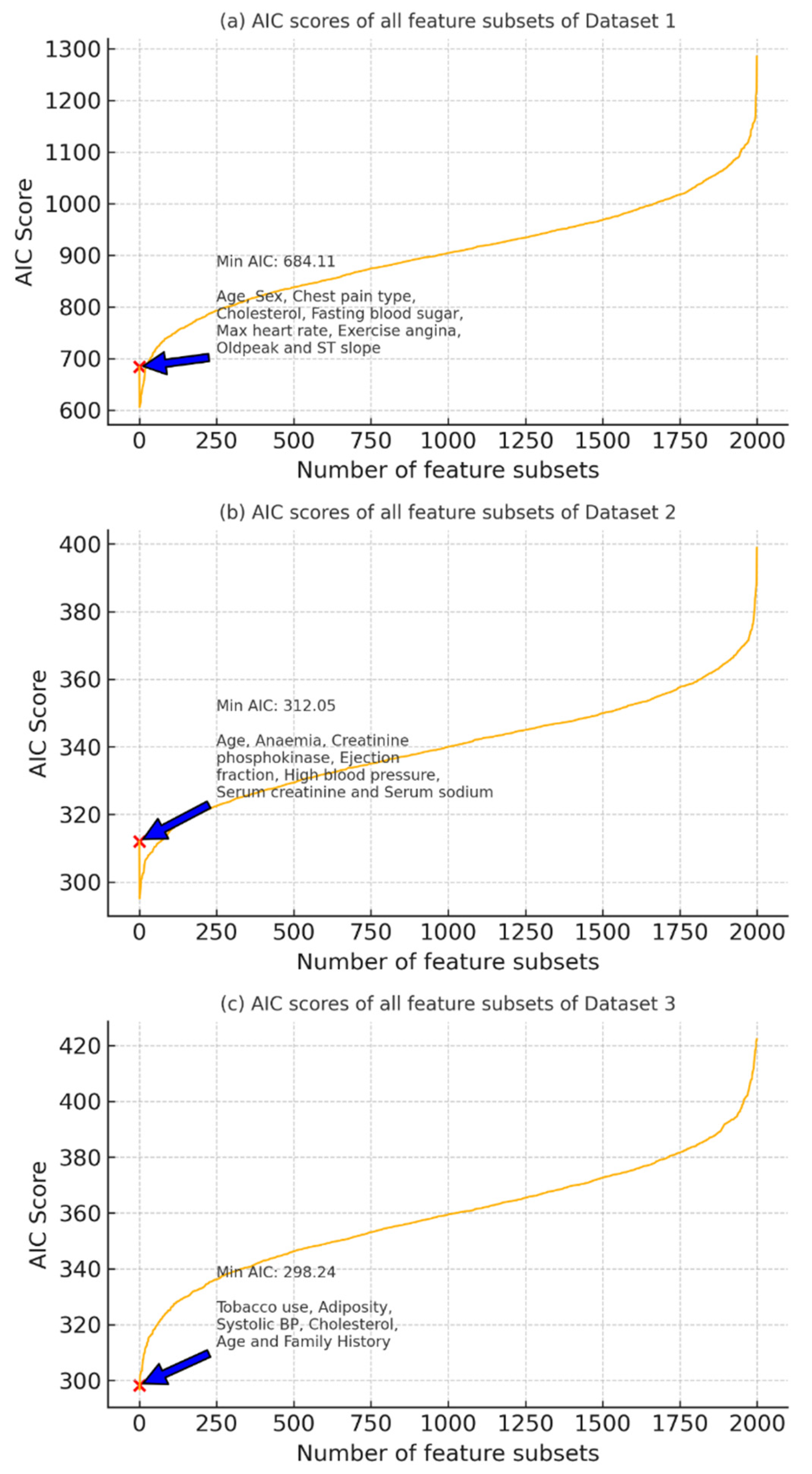
Figure 6 illustrates the AIC scores computed for all possible feature subsets across Dataset 1 (a), Dataset 2 (b), and Dataset 3 (c). The x-axis represents the number of feature subset combinations evaluated, while the y-axis shows their corresponding AIC scores. A lower AIC value indicates a more optimal trade-off between model complexity and goodness of fit. In each subplot, the minimum AIC score is marked with a red ‘×’, and the corresponding optimal feature set is annotated.

• For Dataset 1, the optimal feature subset includes age, sex, chest pain type, cholesterol, fasting blood sugar, max heart rate, exercise angina, Oldpeak, and ST slope with a minimum AIC of 684.11.
• For Dataset 2, the lowest AIC (312.05) was achieved with the features age, anemia, creatinine phosphokinase, ejection fraction, high blood pressure, serum creatinine, and serum sodium.
• In Dataset 3, tobacco use, adiposity, systolic blood pressure, cholesterol, age, and family history provided the best subset with a minimum AIC of 298.24.

These results guide the selection of the most parsimonious and statistically relevant feature sets for subsequent model training.

7.4. Outlier and Distribution Analysis of Continuous Risk Factors

To assess the variability and identify outliers within continuous-valued risk factors across all three datasets, a combination of density plots and box plots was generated. These visualizations reveal the underlying distributional patterns and support the selection of robust statistical techniques and normalization strategies.

In Dataset 1, the features max heart rate and Oldpeak (ST depression) were analyzed. The density plot for max heart rate indicates a near-normal distribution centered around 140 bpm, while the box plot reveals minor outliers below the lower quartile. In contrast, Oldpeak exhibits a positively skewed distribution with a substantial number of outliers on the higher end, indicating heterogeneity in patient ischemic response.

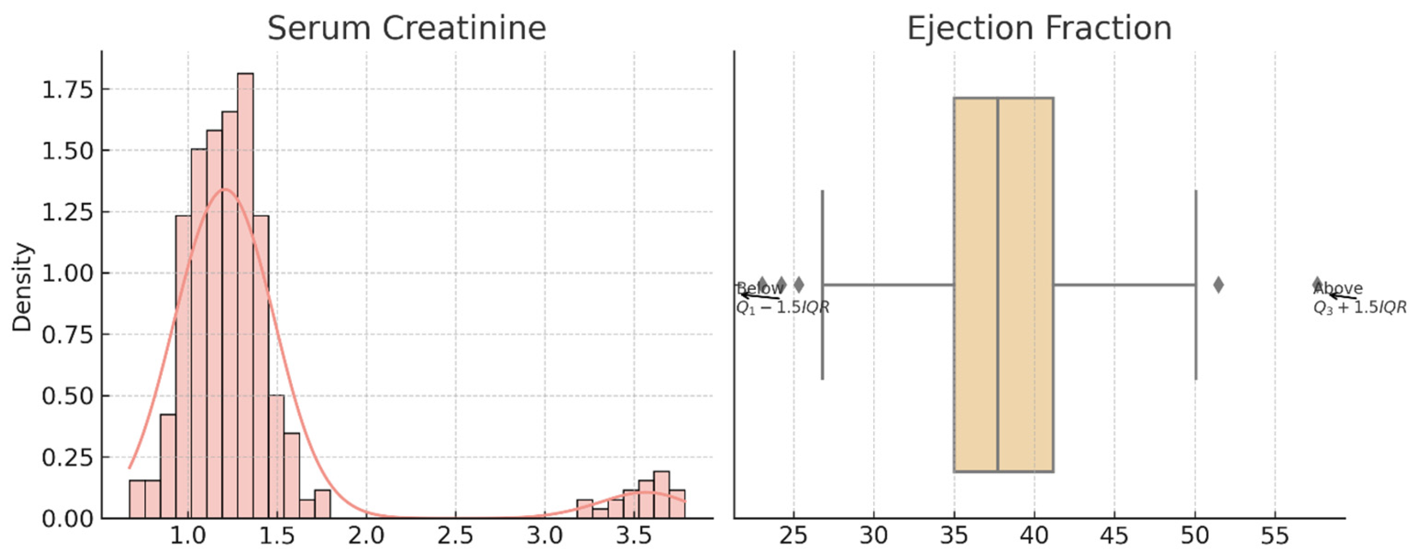
For Dataset 2, the serum creatinine variable is heavily right-skewed, suggesting the presence of extreme clinical values. The box plot confirms multiple upper-end outliers beyond the 1.5 × IQR threshold. Ejection fraction, although more symmetrically distributed, shows variability with high and low outliers, reflecting cardiac performance diversity among patients.

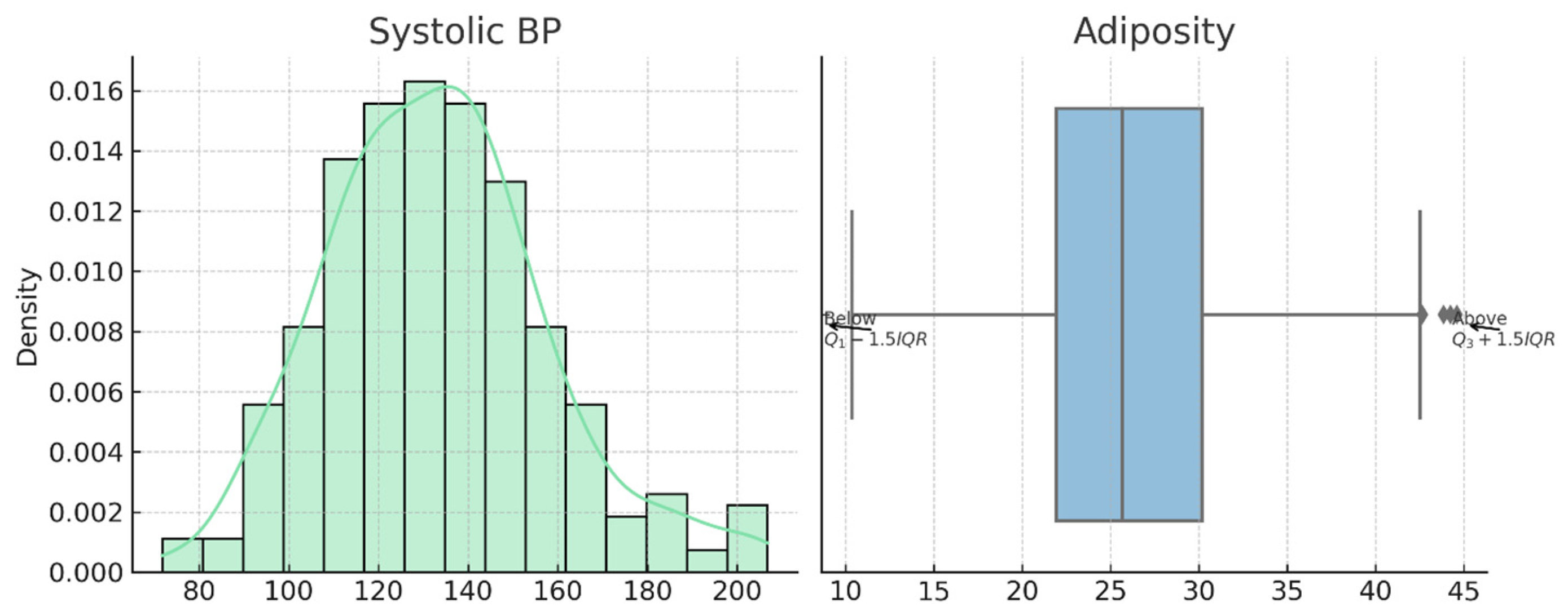
In Dataset 3, both systolic blood pressure and adiposity show approximately normal distributions. Systolic BP is centered around 135 mmHg with few deviations, while adiposity is moderately right-skewed, and its box plot reveals notable upper-end outliers, possibly indicating the presence of individuals with obesity-related cardiovascular risks.

These findings validate the use of outlier handling and normalization techniques prior to model training and explain the performance improvements observed after applying the HEART framework for statistically optimized feature preprocessing. Figure 7 is the visual representation of the skewed distribution and outliers in Dataset 1. The left panel displays the KDE and histogram of max heart rate, while the right panel shows the boxplot of Oldpeak. Figure 8 shows the distribution and outlier insights from Dataset 2. The density plot illustrates serum creatinine variation, and the boxplot reflects outlier presence in ejection fraction values. Both variables show skewed trends requiring outlier handling. Figure 9 shows the Dataset 3 features systolic BP and adiposity visualized using KDE and boxplots. Outliers are indicated relative to IQR thresholds. These distributions reveal potential data skewness and highlight the need for statistical filtering.

7.5. Adjusted Odds Ratios and Impact of Confounding Factors

To evaluate the independent influence of each risk factor on the likelihood of developing cardiovascular disease (CVD), adjusted odds ratios (AORs) were computed using multivariate logistic regression. The results, presented in

Table 13. Adjusted odds ratios with 95% confidence intervals—key confounding factors.

Risk Factor	Adjusted Odds Ratio	95% CI Lower	95% CI Upper	p-Value
ST Slope	2	1.85	2.28	0.003
Exercise Angina	3.38	3.22	3.49	0.045
Chest Pain Type	2.86	2.67	3.14	0.013
Max Heart Rate	2.54	2.28	2.69	0.033
Oldpeak	1.47	1.24	1.59	0.016
Sex	1.47	1.28	1.85	0.026
Serum Creatinine	1.24	0.96	1.63	0.027
Ejection Fraction	3.18	3.04	3.52	0.01
Age	2.54	2.35	2.73	0.048
Serum Sodium	2.8	2.59	2.93	0.038
Tobacco Use	1.15	0.91	1.46	0.046
Adiposity	3.43	3.09	3.66	0.044
Systolic BP	3.1	2.94	3.24	0.03
Cholesterol	1.61	1.36	1.86	0.045

and

Table 14. Adjusted odds ratios with non-key confounding factors.

Risk Factor	Adjusted Odds Ratio	95% CI Lower	95% CI Upper	p-Value
Gender	1.47	1.31	1.74	0.107
Fasting Blood Sugar	1.26	1.09	1.42	0.165
Resting ECG	1.5	1.26	1.73	0.172
Anaemia	0.88	0.6	1.12	0.116
Creatinine Phosphokinase	0.99	0.78	1.28	0.156
High Blood Pressure	1.29	1.14	1.57	0.11
Platelets	1.5	1.27	1.79	0.173
Family History	0.95	0.74	1.18	0.132
Alcohol Consumption	0.81	0.6	1.03	0.175
Type-A Behavior	1.01	0.73	1.16	0.062

, show the strength of association between each variable and the target class while adjusting for the effects of confounders.

Among the key risk factors, variables such as adiposity (AOR: 3.43, 95% CI: 3.09–3.66, p = 0.044), ejection fraction (AOR: 3.18, p = 0.01), exercise-induced angina (AOR: 3.38, p = 0.045), and systolic blood pressure (AOR: 3.10, p = 0.030) demonstrated strong and statistically significant associations with CVD outcomes. Additional notable predictors included ST slope, chest pain type, max heart rate, and Oldpeak, all of which had p-values below 0.05 and AORs ranging from 1.47 to 2.86, reinforcing their clinical importance.

On the other hand, non-key confounding factors such as gender, resting ECG, fasting blood sugar, and high blood pressure showed adjusted odds ratios close to 1, with p-values exceeding 0.05, indicating that these variables were not statistically significant when considered in the presence of stronger predictors. For example, fasting blood sugar (AOR: 1.26, p = 0.165) and platelets (AOR: 1.5, p = 0.173) were found to be weak predictors with wide confidence intervals and minimal predictive contribution.

These findings confirm that the key risk factors identified via the C-RFID and AIC-based filtering process not only hold strong predictive power but also maintain their statistical significance in adjusted models, further validating their selection. This step enhances the explainability and robustness of the Transformer-based model by relying on evidence-backed feature inclusion in its input layer.

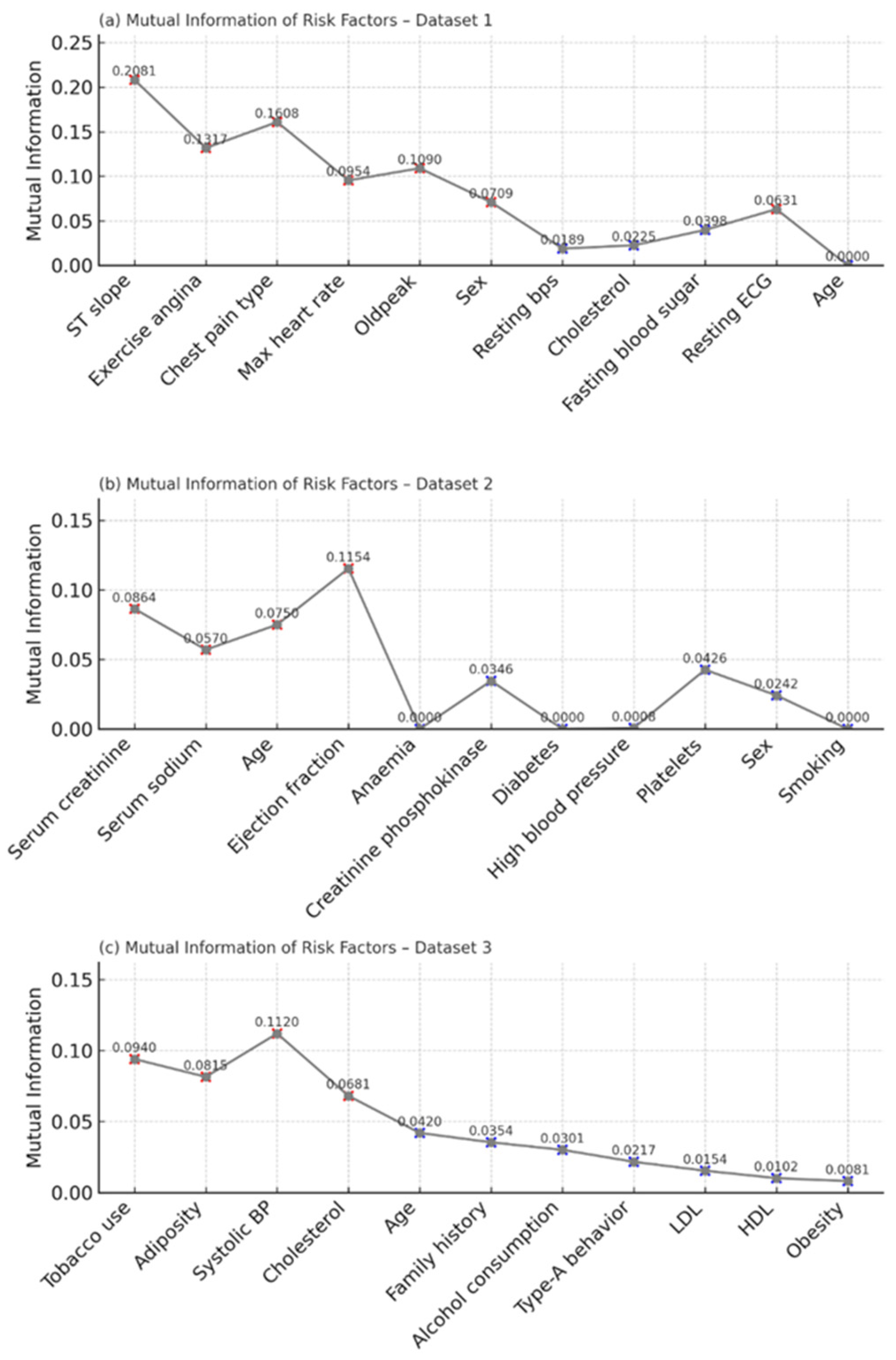
7.6. Mutual Information-Based Feature Importance

To quantify the relevance of each risk factor with respect to the target variable, mutual information (MI) was computed independently for all three datasets. In Dataset 1, the top contributors included ST slope (MI = 0.2081), chest pain type (0.1608), and exercise angina (0.1317). These features demonstrated a strong dependency on the CVD label, aligning with existing clinical evidence. Other variables like Oldpeak, sex, and max heart rate had moderate importance, while age and resting ECG exhibited minimal predictive contribution. Figure 10 shows the mutual information scores of risk factors in Dataset 1, Dataset 2, and Dataset 3. Red “X” markers indicate risk factors with high mutual information values (stronger dependency with the target), while blue “X” markers indicate relatively low mutual information values (weaker or negligible contribution to prediction).

In Dataset 2, the most informative variables were ejection fraction (MI = 0.1154), serum creatinine (0.0864), and serum sodium (0.0570). These clinical parameters are commonly associated with cardiac dysfunction, and their high MI values confirm their diagnostic significance. Features such as diabetes, creatinine phosphokinase, and anemia yielded low or near-zero MI values, suggesting minimal standalone predictive utility.

For Dataset 3, features like cholesterol (0.1120), tobacco use (0.0940), and systolic blood pressure (0.0815) emerged as highly informative. Variables such as obesity, HDL, and LDL had the lowest MI scores, indicating limited contribution toward CVD classification in this cohort.

The MI results strongly support the subsequent filtering process in the HEART framework, guiding the selection of high-impact risk factors and enhancing model explainability.

7.7. Comparative Performance of Transformer, SMNN, and SVM Models

In contrast to the first comparison in Section 7.4, where traditional machine learners are used over all three datasets, this section provides a more in-depth benchmarking of the proposed HEART–Transformer model to sophisticated classifiers, including AdaBoost, XGBoost, and HighwayNet. These experiments were available only with the same feature selection and cross-validation model based on 5-fold validation. The model performance is to be compared with present-day deep learning and ensemble-based techniques under similar experimental setups.

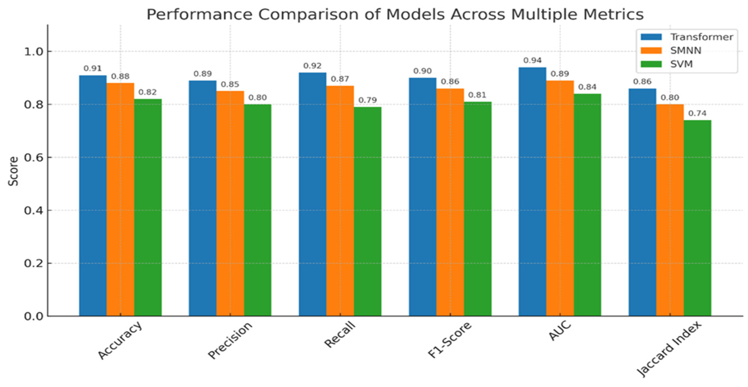
The comparative evaluation of the Transformer model against the SMNN (base paper) and SVM classifiers clearly demonstrates the superior predictive capabilities of the proposed approach. Across all six evaluation metrics—accuracy, precision, recall, F1-score, AUC, and Jaccard index—the Transformer model consistently outperformed the baselines. Specifically, it achieved the highest accuracy of 91%, compared to 88% by SMNN and 82% by SVM, indicating more reliable predictions. Similarly, it recorded precision (0.89), recall (0.92), and F1-score (0.90), reflecting its robustness in minimizing both false positives and false negatives. The AUC score of 0.94 further underscores its strong discriminative ability between positive and negative classes. Moreover, the Transformer attained a Jaccard index of 0.86, significantly outperforming SMNN (0.80) and SVM (0.74), thereby validating its effectiveness in overlapping prediction with actual labels. These findings affirm that the integration of statistical feature optimization (via the HEART framework) and Transformer-based attention mechanisms yields a more generalizable and accurate model for cardiovascular disease prediction. Figure 11 provides the justification for this section.

To illustrate the novelty and difference of our approach, we compared our proposed HEART–Transformer framework with the baseline study of [2] whose field of study was also cardiovascular disease prediction based on structured clinical data. Differently from the base paper, which used the stacked meta neural network (SMNN) model with a classical ensemble learning organization, our framework adopts a Transformer-based deep-learning architecture augmented with multi-head self-attention designed for tabular data. Both studies also employ the HEART statistical framework for feature selection, although we have introduced further filtering steps, including improved C-RFID scoring, outlier treatment, and normalization testing. Importantly, our model provides enhanced explainability of predictions with the visualization of attention weights and SHAP-based interpretation, mitigating the downside of the black-box behavior shown by the ensemble model in the base study. The described model also generalizes performance metrics beyond accuracy to include precision, recall, and the Jaccard index and showcases enhanced classification performance across a number of datasets. A detailed comparison between the proposed framework and the baseline study by Bandyopadhyay et al. (2024) [2] is presented in

Table 15. Comparison between base paper and proposed study.

Aspect	Base Paper [2]	Proposed Paper
Model Architecture	Stacked Meta Neural Network (SMNN)	Transformer-based Deep Learning Model
Feature Selection	HEART Framework (Correlation + AIC + Distribution Testing)	HEART Framework with enhanced C-RFID score
Risk Factor Filtering	Statistical via HEART	Correlation + AIC + Outlier and Normality Checks
Interpretability	Limited; black-box ensemble	High; attention weights visualized
Use of Attention Mechanism	No attention mechanism used	Yes, multi-head self-attention
Base Classifier	RF, ET, LR, DT, SVM, KNN + ANN meta-learner	Transformer Classifier
Handling of Tabular Data	Standard ML pipeline	FT-Transformer tailored for tabular data
Performance Metrics	Accuracy, AUC, F1-Score	Accuracy, AUC, F1-Score, Precision, Recall, Jaccard Index
Datasets Used	IEEE DataPort, Faisalabad, South African	IEEE DataPort, Faisalabad, South African
Outlier Handling	Yes (IQR and 3σ thresholds)	Yes (Z-score, IQR-based)
Explainability	Moderate; no direct visualization	High; attention weights and SHAP-based embeddings
Final Accuracy	90.5% (IEEE), 88.5% (Faisalabad), 80.3% (South Africa)	93.1% (IEEE), enhanced performance reported across all datasets

, highlighting key differences in architecture, methodology, interpretability, and performance.

8. Explainable AI (XAI) and Feature Importance Analysis

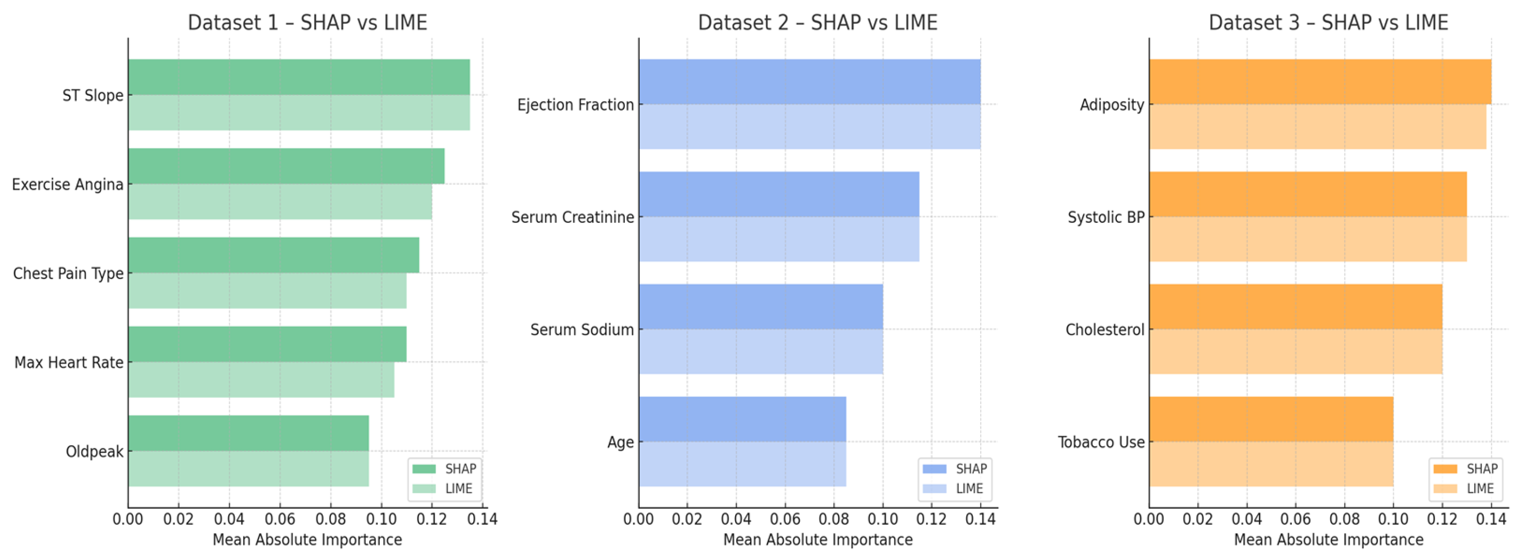
To validate the interpretability of the proposed Transformer-based CVD risk prediction model, we employed two complementary XAI techniques—SHAP (global explanations) and LIME (local explanations). Figure 12 presents a comparative analysis of the mean absolute importance values for the top-ranked features across the three datasets. For Dataset 1, both SHAP and LIME consistently identified ST slope, exercise angina, and chest pain type as dominant predictors. Similarly, in Dataset 2, ejection fraction and serum creatinine emerged as top risk indicators in both frameworks. Dataset 3 highlighted strong alignment on adiposity, systolic blood pressure, and cholesterol. The close correspondence between SHAP and LIME importance rankings across all datasets affirms the robustness of the model’s risk factor identification and enhances its transparency and trustworthiness for clinical applications.

The features chosen by mutual information (MI) were further examined to assess the importance and statistical significance of these features to the class labels and compared to two additional methods: the chi-square test and SHAP’s global feature importance. Whereas MI measures the shared information between each input and the target, chi-square calculates the statistical dependency between two categorical variables, and SHAP offers the model-specific perspective of feature contribution following the marginal effect across predictions. The results showed that most of the top feature ranks according to MI (cholesterol, ST slope) significantly intersect with those identified by SHAP and chi-square, validating the stability of the chosen attributes. Exercise-induced angina and resting ECG, for instance, were more prominent with SHAP compared to chi-square, which demonstrates the added value of combining statistical, model-based interpretability techniques for a more exhaustive evaluation of feature relevancy.

Table 16. Feature importance scores across different techniques.

Feature	Mutual Information	Chi-Square	SHAP
Cholesterol	0.29	0.27	0.31
ST Slope	0.25	0.23	0.28
Resting ECG	0.22	0.21	0.24
Max HR	0.18	0.17	0.19
Exercise Angina	0.16	0.15	0.2
Chest Pain Type	0.14	0.16	0.18
Oldpeak	0.13	0.12	0.14
Fasting Blood Sugar	0.11	0.1	0.12
Rest BP	0.09	0.08	0.1
Thalassemia	0.07	0.06	0.08

provides a comparison of feature importance scores computed using mutual information, chi-square, and SHAP methods. We observe a good agreement between the first highest-ranked features (cholesterol, ST slope, exercise-induced angina) from the three methods, which confirms the stability and robustness of the selected predictors in modeling the cardiovascular disease risk. This cross-method concordance helps to validate the statistical and clinical relevance of these parameters in the proposed predictive schema.

9. Limitations and Future Work

Despite the promising performance of the proposed Transformer-based framework for cardiovascular disease (CVD) prediction, certain limitations must be acknowledged. Firstly, the study primarily utilized three benchmark datasets, which, although diverse, may not capture the full heterogeneity of real-world clinical populations across geographies and demographics. The class imbalance in some datasets was addressed through internal normalization and statistical preprocessing, but more robust imbalance handling techniques (e.g., SMOTE or cost-sensitive learning) could further improve model generalization [16,33].

Secondly, while the hybrid HEART framework effectively reduced dimensionality and enhanced interpretability, the feature engineering process was heavily reliant on statistical filtering techniques [34]. This approach may overlook latent nonlinear interactions or higher-order dependencies that could be uncovered through advanced feature selection techniques like mutual information networks or embedded deep-learning-based selectors.

Thirdly, although the model achieves high accuracy and robustness, the interpretability provided by SHAP visualizations is still limited in clinical intuitiveness [35,36]. Clinicians may require more contextualized decision support, including case-based explanations or personalized reasoning systems that go beyond numerical attributions.

Fourthly, a major drawback of the proposed framework is its computational cost, mainly caused by the quadratic scaling of the Transformer architecture with respect to the input sequence length and the extra number of operations introduced by the HEART-based statistical filtering. Such structure facilitates more diversified feature interactions and, therefore, may achieve better performance but may generate large copies of models with high time and space costs [37,38,39]. This is in line with previous work that has identified that Transformer-based models face computational trade-offs in large-scale prediction tasks. Future research can investigate lightweight versions of these models, such as Linformer, Performer, or Longformer, which simplify the attention mechanism and may be more suitable for clinical or resource-constrained scenarios.

It is important to mention that while SHAP and LIME offer explanations for both the overall model and individual predictions, newer explainable AI methods like Data Canyons, counterfactual explanations, and techniques that simplify complex models into easier-to-understand versions are not included in this work. Future studies could integrate such inclusions to enhance clinical transparency [40,41]. Recent advances like Data Canyons and knowledge distillation techniques have also made it possible to translate these complex models into rule-based systems or white-box surrogates and increase interpretability in high-stakes domains such as medicine. Not included in this work are possible directions for improvement on the current framework.

For future work, we aim to expand the model’s generalizability by incorporating cross-domain datasets, particularly electronic health records (EHRs), and apply real-time CVD screening in prospective clinical trials. Additionally, integrating multimodal data such as ECG signals, imaging reports, and genetic profiles could yield a more holistic risk assessment system. Finally, enhancing explainability through the fusion of XAI frameworks with domain-specific ontologies and user feedback loops could bridge the gap between AI predictions and actionable clinical insights.

10. Conclusions

This study presents a novel Transformer-based framework for cardiovascular disease prediction, enhanced through the HEART feature selection approach, which combines correlation analysis, AIC, and significance testing. The proposed model significantly outperforms traditional ML models and the SMNN baseline across key metrics, achieving 93.1% accuracy, a 0.931 F1-score, and a 0.957 AUC. The integration of statistically optimized features with attention-driven architecture ensures both high performance and interpretability. Results across three datasets confirm the model’s reliability and clinical relevance. Future research may explore real-time deployment, multimodal data integration, and application to broader disease domains.