Abstract
This paper extends the multipoint flux approximation (MPFA-O) method to model coupled pressure and saturation dynamics in subsurface reservoirs with heterogeneous anisotropic permeability and non-K-orthogonal grids. The MPFA method is widely used for reservoir simulation to address the limitations of the two-point flux approximation (TPFA), particularly in scenarios involving full-tensor permeability and strong anisotropy. However, the MPFA-O method is known to suffer from spurious oscillations and numerical instability, especially in high-anisotropy scenarios. Existing stability-enhancing techniques, such as optimal quadrature schemes and flux-splitting methods, mitigate these issues but are computationally expensive and do not always ensure monotonicity or oscillation-free solutions. Building upon prior advancements in the MPFA-O method for pressure equations, this work incorporates the saturation equation to enable the simulation of a coupled multiphase flow in porous media. A unified framework is developed to address stability challenges associated with the tight coupling of pressure and saturation fields while ensuring local conservation and accuracy in the presence of full-tensor permeability. The proposed method introduces stability-enhancing modifications, including a local rotation transformation, to mitigate spurious oscillations and preserve physical principles such as monotonicity and the maximum principle. Numerical experiments on heterogeneous, anisotropic domains with non-K-orthogonal grids validate the robustness and accuracy of the extended MPFA-O method. The results demonstrate improved stability and performance in capturing the complex interactions between pressure and saturation fields, offering a significant advancement in subsurface reservoir modeling. This work provides a reliable and efficient tool for simulating coupled flow and transport processes, with applications in CO2 storage, hydrogen storage, geothermal energy, and hydrocarbon recovery.
1. Introduction
Subsurface reservoirs are vital for numerous energy and environmental applications, including CO2 sequestration, hydrogen storage, geothermal energy extraction, and hydrocarbon production. These systems are inherently complex, involving heterogeneous geological formations with intricate geometries, sharp contrasts in permeability, and anisotropic properties. Accurately modeling the flow and transport of fluids in such settings requires advanced numerical methods capable of addressing these challenges while maintaining computational efficiency and stability. The standard workflow for developing a computational model involves the formulation of a rigorous mathematical framework that accurately describes the underlying physical phenomena, followed by its translation into a numerical model amenable to a computational solution [1].
Among the various numerical methods, finite volume methods (FVMs) have emerged as a robust approach to modeling subsurface flow problems. They are favored for their ability to conserve fluxes both locally and globally [2,3], making them particularly suited for problems involving discontinuous material properties and anisotropic permeability. Standard methods like the two-point flux approximation (TPFA) are widely used but exhibit significant limitations on non-K-orthogonal grids or in the presence of full-tensor permeability fields [4]. This has motivated the development of more sophisticated methods, such as the multipoint flux approximation (MPFA) family [5], which addresses many of the shortcomings of TPFA by incorporating additional support points to capture diagonal and off-diagonal flux components.
The MPFA-O method is one of the most commonly used variants within the MPFA framework due to its generality and accuracy. By incorporating contributions from diagonal neighbors, it effectively handles full-tensor permeability on non-K-orthogonal grids. However, its application is not without challenges. In the presence of strong anisotropy or highly misaligned grids, the MPFA-O method can produce spurious oscillations, violate the maximum principle, and exhibit non-monotonic behavior [6]. These numerical artifacts undermine the physical realism of the simulation and limit the method’s applicability in practical reservoir modeling scenarios. Several approaches, including reduced stencils like the MPFA-U [7] and MPFA-D [8] as well as flux-splitting techniques [9,10], have been proposed to address these issues, but they often come with trade-offs in terms of computational complexity, accuracy, or generality.
While significant progress has been made in improving the stability and accuracy of pressure equation solvers, modeling coupled multiphase flows in subsurface reservoirs remains a major challenge [11,12]. In such systems, the pressure and saturation equations are tightly coupled, with the pressure field driving fluid movement and the saturation field influencing pressure dynamics through relative permeability and capillary pressure effects. The inclusion of the saturation equation introduces additional nonlinearities and interdependencies that complicate the numerical solution process. Accurately capturing the coupled behavior of these equations is critical for simulating real-world phenomena, such as waterflooding in oil reservoirs, gas injection for enhanced recovery, and the migration of CO2 plumes in sequestration projects.
Saturation dynamics are governed by transport equations that describe the movement and redistribution of fluid phases in porous media. These equations are highly nonlinear and often exhibit sharp fronts or discontinuities due to the heterogeneous and anisotropic nature of subsurface reservoirs. Numerical methods for solving saturation equations must ensure physical accuracy while preserving properties like monotonicity and positivity, especially in the context of multiphase flows. Standard methods often struggle to balance these requirements, leading to numerical instabilities or excessive computational cost. Increasing the method’s efficiency with multigrid methods [13], adaptive local mesh refinement [14], and parallelization [15] is a viable approach. However, we strived to maintain the simplicity of numerical software and maximize the method’s inherent versatility, accuracy, and computational efficiency. The emerging field of quantum computing has the potential to enhance the solution of differential equations [16] and is theoretically expected to provide a polynomial speedup for finite element methods [17].
The MPFA-O method, which has been extensively used for solving pressure equations, offers an attractive foundation for extending numerical modeling capabilities to include saturation dynamics. However, integrating the saturation equation into the MPFA-O framework is nontrivial and requires addressing several key aspects. These include ensuring stability and accuracy in the presence of strong coupling between pressure and saturation fields, handling full-tensor permeability with complex geological layering, and maintaining computational efficiency on large-scale problems with fine resolutions.
The improved MPFA approach introduced in this study extends the stability-enhancing modifications applied to pressure computations in previous work [18] to the saturation equation, addressing numerical stability and spurious oscillations on non-K-orthogonal grids. Such grids refer to grid configurations where the connection vector between adjacent cell centers is not aligned with the principal directions of the permeability tensor. This misalignment can lead to significant numerical errors in standard MPFA methods, where the discretization of the saturation equation suffers from unstable saturation profiles, particularly in highly anisotropic domains. To mitigate these issues, the improved method integrates local permeability tensor rotations and improved flux approximations, ensuring a more accurate representation of fluid transport dynamics.
The primary contributions of this study are threefold: (1) the formulation of a unified framework that seamlessly integrates the pressure and saturation equations within the MPFA-O method, (2) the implementation of stability-enhancing techniques to mitigate spurious oscillations and ensure monotonicity in the numerical solution, and (3) the demonstration of the method’s performance through numerical experiments on heterogeneous, anisotropic domains using non-K-orthogonal grids. By addressing these objectives, the proposed method offers a significant step forward in the development of reliable and efficient tools for subsurface reservoir simulation.
The motivation for this work stems from the increasing demand for accurate and efficient modeling techniques that can handle the complexities of real-world reservoirs. Geological formations often exhibit significant variations in permeability and anisotropy due to factors like cross-bedding, fracturing, and diagenetic processes [19]. These variations result in full-tensor permeability fields that are rotated relative to the computational grid, posing challenges for traditional numerical methods. In addition, the upscaling of geological properties from fine-scale measurements to coarse-scale simulation grids introduces further complexities, including the emergence of non-K-orthogonal permeability tensors [20]. These factors necessitate the use of advanced numerical methods capable of capturing the intricate interactions between pressure and saturation dynamics while accommodating the geometric and material complexities of the reservoir.
The inclusion of the saturation equation in the MPFA-O framework represents a natural extension of its capabilities. By enabling the simulation of coupled multiphase flow processes, the proposed method provides a more comprehensive tool for understanding and predicting subsurface behavior. This is particularly important in the context of emerging applications like CO2 storage and hydrogen storage, where the interaction between the pressure and saturation fields plays a key role in determining the success and safety of the operation.
2. Two-Phase Flow
In this paper, we consider a 2D immiscible incompressible two-phase fluid flow through static porous media. Domain is chosen to be a 1 × 1 square in the x and y directions:
No-flow boundary conditions (BCs) were added around the domain except for the places where the source terms are specified on the boundary. For the initial condition (IC), we assume that the reservoir is predominantly filled with the non-wetting phase, with the wetting phase saturation being negligibly small. While in reality, phase saturations are rarely exactly 0% or 100% due to capillary effects and residual saturations. This assumption simplifies the numerical treatment and aligns with typical reservoir simulation practices. Values for the irreducible saturation of wetting and non-wetting phases are set to be both zero; viscosities to 0.44 mPa·s and 0.52 mPa·s, respectively; and densities to 1000 kg/m3 and 800 kg/m3.
2.1. Capillary Pressure
A two-phase interaction in a porous media creates capillary action due to wettability effects, which promotes imbalance at the interfaces of each fluid. This is due to the adhesive and cohesive forces that attract each phase to the solid matrix and to each other, respectively. Generally, the interface between phases is curved due to specific physics at the pore level, which is what defines whether the phase is wetting (angle between solid matrix and interface is <90°) or non-wetting (angle is >90°). The pressure between two phases is related via Equation (2):
where is the pressure of a non-wetting phase, is the pressure of a wetting phase, and is the capillary pressure. A framework for modeling capillary pressure in saturated porous media is presented in [21].
Capillary pressure can be dependent on a few variables like temperature, fluid composition, etc.; however, the most prominent one is saturation. The relationship can be derived from direct measurement [22] or from heuristic functional relationships [21,23,24].
Capillary forces are significant enough to mention, as they can even be linked to causing the hysteresis seen in cyclic reservoir drainage/imbibition [25]. However, in a typical injector/producer system, capillary forces are relatively small and can be neglected. This means that we can assume and use a general pressure quantity p:
2.2. Darcy Equation
The notion of flow through porous media is specifically described by the Darcy flow equation. For a two-phase flow problem, it takes the following shape:
where denotes either a wetting or non-wetting phase, is the fluid flow vector of the phase , K is the permeability tensor of a solid matrix, is the relative permeability concerning phase (see Section 2.3), is the viscosity of phase , is the pressure gradient of phase , is the density of phase , and g is the gravitational constant. A theoretical analysis of the semi-empirical formulation of Darcy’s law is provided in [26].
There is also a significant notion of mobility of each phase, which can be introduced as follows:
We consider the problem to be observed from the top of a reservoir, which means that the gravity term cancels out. Coupling this with the mobility term introduction and Equation (3), which lets us use only one pressure quantity, we can rewrite the Darcy flow as follows:
Adding the mobilities of all of the phases produces the total mobility :
This is used to define the fractional flow of each phase , which describes the part of phase that contributes to the total flow (see Equation (22)):
2.3. Permeability Tensor and Relative Permeability
Permeability and relative permeability [27,28] are two different quantities that together describe how a specific phase acts under a pressure gradient.
Permeability describes how easily fluids can move through porous media like rocks or soil, and it is expressed as a tensor due to its ability to give a directional magnitude for flow in different directions in space. The relative permeability of a phase is not determined by the solid matrix of the porous medium itself, but rather by the presence of other fluid phases within the pores, which obstruct or interfere with the flow pathways. Its value ranges in , and it is a function of saturation (based on the capillary pressure–saturation relationship [29]) considering an immiscible flow [30]. Relative permeability can have many different analytical expressions or be defined as a piecewise function using empirical table data. Here, we use simple definitions:
where is the saturation of the wetting phase.
In this work, our main focus lies on situations where the anisotropic permeability tensor K is not K-orthogonal, i.e., when the principal directions of the permeability tensor do not coincide with the coordinate axes of the computational grid. This is achieved by rotating the orthogonal permeability tensor by degrees using an anticlockwise rotational matrix :
For changing the computational reference in a later flux calculation, we also introduce the clockwise rotational matrix and name it :
2.4. Continuity Equation
Continuity equation states that the mass of the fluid in the model should not be able to appear and disappear at random, i.e., it should be conserved, unless stated otherwise:
where denotes the solid matrix porosity, is the saturation of phase , and is a source term that depicts divergence. An introduction of the continuity equation in the context of multiphase flow can be found in [1].
Reading from left to right, this mass conservation Equation (12) describes how the mass of the phase changes in time given certain fluxes through elementary volume interfaces. On the RHS, there is a source term that describes the generation of fluid, in cases of injection/production, flows from the third dimension, etc.
Expanding the time derivative of the first term and spacial derivative of the second term provides the following:
For simplicity, we assume that porosity does not change with time and has a value of 0.5, which eliminates the first term. An incompressible case also assumes pressure to be constant, which rules out the gradient and temporal derivatives of the densities of both phases as well:
The final form of the continuity equation in this paper is obtained by dividing both sides by :
The continuity equation enforces the fundamental law of mass conservation, and for discrete solutions, it is usually divided into two separate equations. Equation (15) is what we use for the saturation calculation, while the pressure Equation (19) provides the preliminaries for the solution. Alternating between the pressure and saturation solution for each iteration is what defines the IMPES method—implicit formulation for pressure, explicit for saturation.
2.5. Pressure Equation
In order to derive the pressure equation, we write out Equation (15) in full:
Given that only two phases are considered, i.e., , the rate of change of the saturation phase is the same as that of the saturation phase but negative:
Adding up the resulting equations to produce a single pressure equation yields the following:
Introducing a new general flow and source terms respectively yields the following:
These can be used to simplify the pressure Equation (19) into
A fractional flow can be used to obtain the flow of each phase:
3. Numerical Methodology
3.1. Solving for Pressure
One of the MPFA variations is used to solve the pressure Equation (21), which is thoroughly described in a recent paper [18]. This methodology focuses on addressing the challenges associated with high anisotropy on non-K-orthogonal grids in subsurface reservoir simulations. Specifically, it improves upon the MPFA-O method by incorporating the anisotropic characteristics of the permeability tensor at the local cell level. The key advancement of the improved MPFA framework ensures that the corrected pressure gradients preserve the physical integrity of fluid movement by properly aligning the computational grid with the tensor axes (see Figure 1).
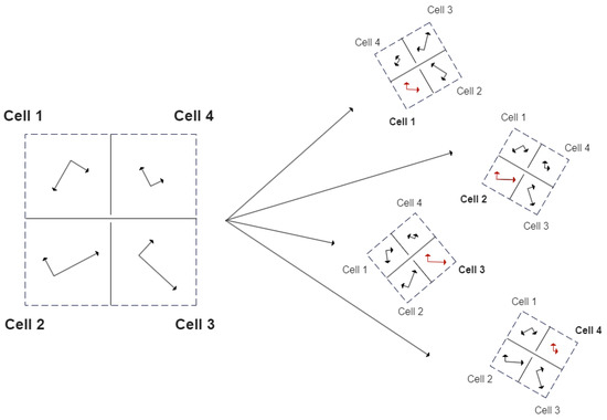
Figure 1.
A representative interaction volume is illustrated on the left, positioned within the physical space, where flux coefficients for its half-edges are to be computed. For each cell, a local rotation is applied to align the permeability tensor with the computational space, facilitating accurate flux calculations on the associated half-edges. The right side of the figure presents the four rotated cases, demonstrating how each cell’s tensor is aligned to ensure consistency within the numerical framework.
The method comes from a vast family of finite volume methods that enforce the continuity of fluxes and pressures across control volumes. For this particular methodology, permeability tensors may be anisotropic and rotated by a certain angle. Interaction volumes are defined for each vertex and contain four half-edges of the neighboring cells (see Figure 2). Within each cell of the interaction volume, the pressure gradient is bilinearly approximated using three reference points: the cell center and two points located at the corresponding half-edges. These gradients are then used to compute the fluxes within each involved cell according to Darcy’s law. To ensure that the local physics of flow is respected, the gradient transmissibility matrices are rotated appropriately. By enforcing flux continuity between neighboring cells and applying local mass conservation, a set of equations is constructed. These equations are then ridden of intermediate variables and used to fill the global system matrix suitable for solving the full flow problem.
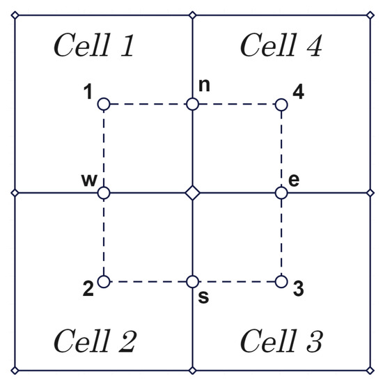
Figure 2.
Local representation of 4 cells around a grid point.
The method was validated through a comparison with an analytical solution and a series of numerical tests as well as a convergence study, confirming its accuracy and performance. It exhibited notable stability improvements over the standard MPFA-O approach, ensuring robust and accurate solutions even under extreme conditions such as high subsurface heterogeneity.
Validation in this paper is performed through a series of test cases, comparing the standard MPFA and improved MPFA approaches in homogeneous, anisotropic, and heterogeneous domains. The results demonstrate improved accuracy in saturation front propagation and more physically consistent production profiles.
We note that the computational efficiency remains unchanged across the compared MPFA-O implementations, as the underlying stencil and system assembly are identical. The primary advancement is the correct rotation treatment of the permeability tensor.
3.2. Solving for Saturation
The saturation equation is solved after the pressure is already known and only for one phase, which we consider to be the wetting one. Discretizing the domain into a finite amount N of cells , and applying the finite difference approximation yields an explicit formulation of the equation:
where is the average porosity of cell , is the time step, is the cell-average of the wetting phase saturation at time k in cell , is the cell area, is the wetting phase flux from the cell to the neighboring cell through their interface, and is the source term of cell .
To evaluate , we consider Equation (24):
where is a vector that is perpendicular to the interface between cells and and has the same length, and is fractional flow value at the interface (see Equation (25)). MPFA calculations are made on half-edges rather than the whole interfaces between two neighboring cells, so this definition is general, but later we define a more specific definition.
Evaluating the flux at the interface between neighboring cells becomes challenging because the fractional flow depends on saturation. It is not obvious which of the neighboring cell’s fractional flow value ( or ) should be used to calculate the phase flow vector (see Equation (22)), since neighboring cells can have different saturations. Typically, fractional flow at interface is chosen from the cell, from which flow v is pointing outwards:
Given certain boundary and initial conditions, it is possible to evolve the saturation solution in time by expressing the saturation at the next time step:
3.3. Solving for Flux
Evaluation of flux at the interface between neighboring cells is possible by reconstructing the pressure gradient, which can be done through conventional means like using least squares or Gauss procedures. We propose a much more MPFA-friendly approach by backtracking some of the calculations in the pressure solver and leveraging certain assumptions. This is the key for introducing the same concept of a local computational grid rotation for flux calculation as was performed with pressure.
Apart from the boundary, each grid point is a member of 4 cells: 1 through 4 locally (see Figure 2). At the middle of the interfaces between two neighboring cells, we mark w, s, e, and n points that divide the interface into two half-edges. Connecting these local points 1, w, 2, s, 3, e, 4, n, 1 in order defines an area called an interaction volume. Four half-edge fluxes of different edges are calculated per interaction volume (dashed area in Figure 2). In order to obtain the remaining half-edge fluxes to complete the four fluxes through these interfaces, another interaction volume has to be taken. Adding both half-edge fluxes of the same interface results in a complete flux through an interface between two neighboring cells .
One of the assumptions of MPFA is that the pressure p changes bilinearly by some constant pressure gradient along the entirety of the cell and can be expressed as such (see [18]):
where x and y refer to center coordinates of the cell centers or the w, s, e, and n points on the half-edges. The primary quantities of interest here are the pressures at the centers of the cells and the pressures at the middle points of interfaces , , , and .
The MPFA procedure allows us to calculate the pressure values at the cell faces , , , and using the pressure values at the cell centers that were obtained when solving the pressure equation. These can be used to evaluate the flow through the half-edges by using the Darcy equation. The only modification is the rotational matrix added in front of the gradient:
Dot product is used between the resulting flows and the normal vectors to obtain the half-edge fluxes. These fluxes for the wetting phase can be found using an appropriate fractional flow function (see Equation (24)):
where , , , and are orthogonal vectors of each half-edge of the same size as its length.
Since interaction volumes do not extend to the sides of the grid, the flux at the boundary cells would be lower than it should be, i.e., interfaces between the cells that are located at the same boundary will only have one of the two required half-edge fluxes. To account for the missing flux, the present one is doubled.
3.4. Initial Conditions and Source Terms
The initial condition of the domain is set to be fully saturated by a non-wetting phase. The introduction or retraction of the fluid into a cell acts from outside of the domain and, thus, has to be added via the source term (see Equation (26)). In this article, each cell source is introduced from the pressure constraints, which implies that all of the values are obtained from the pressure equation. Positive values indicate injection and negative values indicate production. Injection is made only using the wetting phase, so there is no fractional flow for the injection cell, while the production cell can take up mixed fluid. Using these conditions, Equation (26) can be further refined:
3.5. General IMPES Sequence
There are a few different approaches to solving the given system of equations like IMPES, sequential solution methods [31], adaptive implicit methods [32], etc. This paper uses the IMPES approach, see Algorithm 1, which suggests alternating between pressure and saturation solution for each iteration—implicit formulation for pressure, explicit for saturation. The general workflow of this method can be summed up as follows:
| Algorithm 1 Calculate |
|
3.6. Courant–Friedrichs–Lewy Condition
The Courant–Friedrichs–Lewy (CFL) condition is used to ensure that the numerical method would converge to a solution when solving certain partial differential equations explicitly. Since the IMPES method calculates the saturation values explicitly, the CFL condition does apply here. This comes in the form of limiting the time step size to be under a certain value. The heuristic CFL condition for the first-order upwind scheme for the heterogeneous domain is provided in [12]:
where marks the total flow into the cell.
For this article, we set the fractional flow of the wetting phase to be (see Equations (5), (7), (8) and (9)) as follows:
Its derivative, then, is as follows:
To reduce the amount of calculations required, we can take the maximum possible value for the derivative in the range of , which, rounded up, is 2.01.
4. Results
In this section, the standard MPFA and the improved MPFA are compared. Each comparison figure presents three graphs from left to right: pressure distribution, flow field, and wetting phase saturation distribution, all evaluated at . Flow field arrows are scaled down and color-coded by magnitude to reduce visual clutter. High-magnitude flows are shown in red, low-magnitude flows in blue, and intermediate values in darker shades. A colorbar is omitted to conserve figure space, but relative magnitudes are visually distinguishable.
Figure 3 represents the base case, where the permeability tensor is defined as within a homogeneous domain. This result is can either be obtained by using the standard MPFA without applying any permeability tensor rotation (see Figure 3a) or the improved MPFA with any tensor rotation (see Figure 3b and Figure 4b). Since the two methods are computationally identical on K-orthogonal grids, they produce the same results in all three graphs, leading to identical saturation production profiles (see Figure 5).
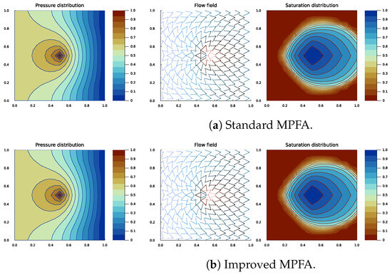
Figure 3.
Pressure, flow, and saturation plots at the last time step of the standard MPFA. The domain is homogeneous with an unrotated isotropic permeability tensor K.
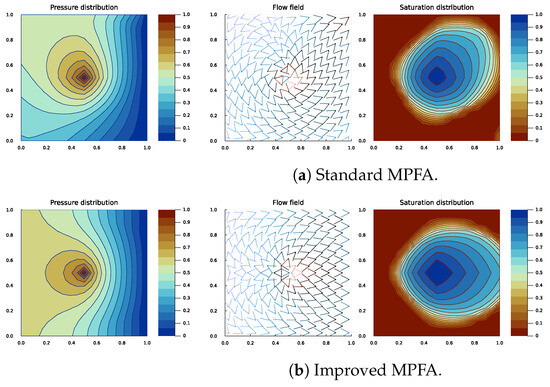
Figure 4.
Pressure, flow, and saturation plots at the last time step of the standard MPFA. The domain is homogeneous with a rotated isotropic permeability tensor K.
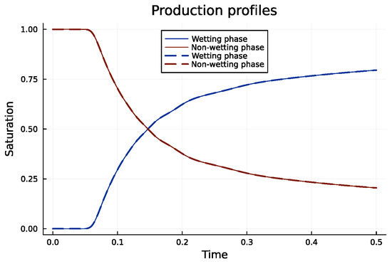
Figure 5.
Saturation production profiles for both methods, with the standard MPFA method depicted as a dashed line and the improved MPFA method as a continuous line. The domain is homogeneous with an unrotated isotropic permeability tensor K.
4.1. Rotational Effect
In this subsection, we show what discrepancies the standard MPFA exhibits when the permeability tensor is rotated by anticlockwise and becomes the following:
The permeability inside the media remains effectively the same; however, the standard MPFA shows a clear rotational effect in its solution (see Figure 4a), whereas the improved MPFA (Figure 4b) produces the same graph as the base case and preserves this logic.
The production profiles (Figure 6) reveal that the standard MPFA method predicts early production of the wetting phase, which contradicts the imposed simulation conditions. Additionally, the standard MPFA curves exhibit discontinuities, characterized by three distinct segments (separated by black dots), whereas the flow physics suggest only two: before and after the wetting phase reaches the producers. In contrast, the improved MPFA method correctly captures this transition. Furthermore, the standard MPFA overestimates the breakthrough time of the wetting phase and consistently predicts a higher non-wetting phase profile throughout most of the simulation.
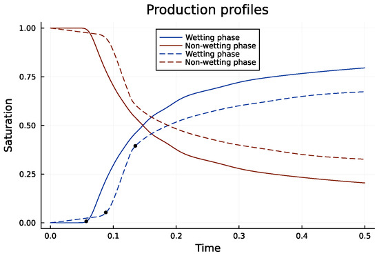
Figure 6.
Saturation production profiles for both methods, with the standard MPFA method depicted as a dashed line and the improved MPFA method as a continuous line. The domain is homogeneous with a rotated isotropic permeability tensor K.
4.2. Anisotropy Effect
In this subsection, we add anisotropy to the rotated case. A comparison is made in Figure 7 by presenting side-by-side results of the two methods.
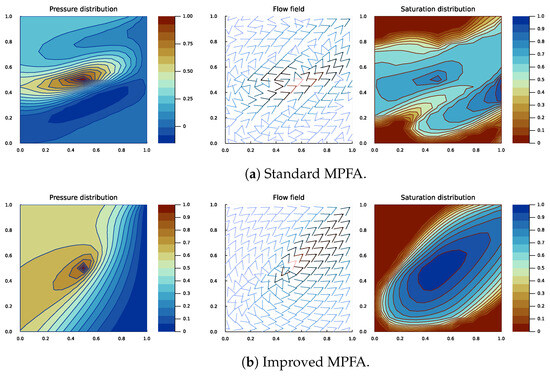
Figure 7.
Pressure, flow, and saturation plots at the last time step. The domain is homogeneous with a rotated anisotropic permeability tensor K.
The permeability tensor rotated by anticlockwise introduces numerical instability in the standard MPFA method, leading to oscillations in the pressure solution (see Figure 7a). This instability manifests as an erratic flow field and the emergence of spurious sources along the right boundary of the saturation distribution. The effect is also evident in the production profiles (see Figure 8), where the standard MPFA lacks a well-defined pre-breakthrough period, instead exhibiting an abrupt decline in the non-wetting phase saturation from the onset of the simulation. In contrast, the improved method maintains physical consistency, predicting a more gradual transition, and yields a higher non-wetting phase production for most of the simulation duration.
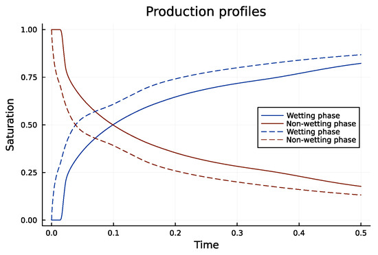
Figure 8.
Saturation production profiles for both methods, with the standard MPFA method depicted as a dashed line and the improved MPFA method as a continuous line. The domain is homogeneous with a rotated anisotropic permeability tensor K.
4.3. Layered Domain
The final test is conducted on a heterogeneous permeability domain, as described in Figure 9, featuring an anisotropic high-permeability layer intruding through the middle of the domain. This layer facilitates preferential flow pathways, creating a “highway” effect that is expected to be reflected in the pressure distribution. However, the standard MPFA pressure solution (Figure 10a) exhibits reduced sensitivity to this permeability variation compared to the improved method (Figure 10b).
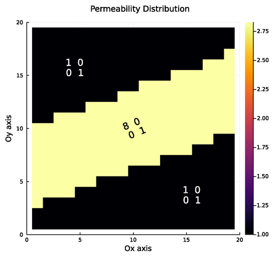
Figure 9.
Permeability distribution of the “layered” case. Matrices in the graph represent the permeability tensors with their rotations accordingly. The bright layer makes a angle with the horizontal and so does its permeability tensor. Values of the graph represent the determinant of K in each cell.
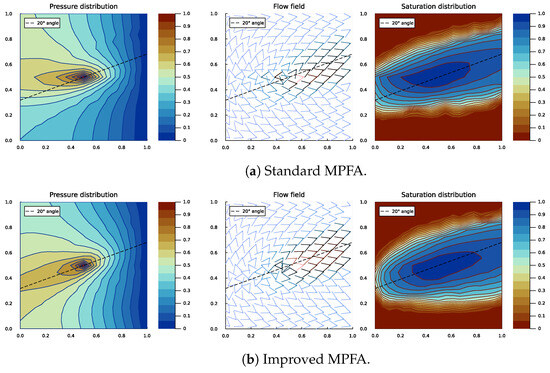
Figure 10.
Pressure, flow, and saturation plots at the last time step. The domain is heterogeneous with a rotated anisotropic permeability tensor K at the permeable layer and an unrotated isotropic permeability tensor K elsewhere.
As a result, the standard MPFA generates a more horizontally oriented flow field and a less diffused, elongated saturation front. The wetting phase reaches the left model boundary earlier and displays distortions in its distribution. Despite the differences in pressure and flow fields, the saturation distribution produced by the standard MPFA initially maintains a general inclination with respect to the horizontal and closely aligns with the improved method in terms of early-stage production profiles (Figure 11). However, as the simulation progresses, the saturation curves diverge, with the standard MPFA predicting a higher non-wetting phase saturation cut over time.
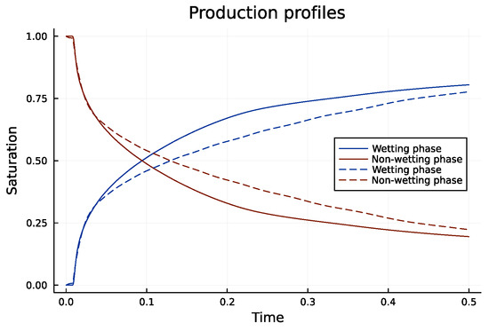
Figure 11.
Saturation production profiles for both methods, with the standard MPFA method depicted as a dashed line and the improved MPFA method as a continuous line. The domain is heterogeneous with a rotated anisotropic permeability tensor K at the permeable layer and an unrotated isotropic permeability tensor K elsewhere.
4.4. Convergence
In the previous paper [18], it was shown that the pressure solution self-converges on highly anisotropic non-K-orthogonal grids. Figure 12 shows the same for saturation, where the grids vary from to , with the reference solution being on a grid.
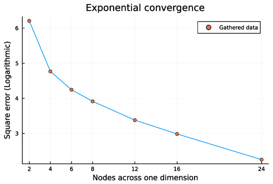
Figure 12.
Logarithmic square error graph illustrating improved MPFA-O solution tendency towards self-convergence.
5. Conclusions
This study builds upon the advancements made in the multipoint flux approximation (MPFA-O) method for subsurface reservoir simulations, extending its application to coupled pressure and saturation dynamics. The newly developed methodology integrates the saturation equation into the MPFA framework, addressing key challenges associated with anisotropic and heterogeneous permeability distributions, particularly on non-K-orthogonal grids. By leveraging a local rotation transformation for the permeability tensor, the improved method exhibits enhanced stability and accuracy while maintaining the maximum principle and monotonicity.
The main novelty of this study lies in extending the previously introduced MPFA-O methodology [18] (which was applied solely to the pressure equation) to the full two-phase flow framework, including the saturation equation. This also required introducing a consistent and physically meaningful computation of the flow (Darcy velocity) field from the pressure solution, which is necessary for accurate saturation updates. Furthermore, we showed that improper handling of the rotated permeability tensor significantly alters the simulated saturation front, underscoring the importance of the correction we propose.
The improved MPFA demonstrates significant advantages over the standard MPFA approach. The base case results confirm that the improved MPFA preserves the accuracy of the original formulation for isotropic homogeneous permeability tensors, regardless of tensor rotation. However, when introducing anisotropy or heterogeneity, the standard MPFA shows instability, such as spurious oscillations in the pressure solution and distortion in saturation fields. Conversely, the improved method remains stable and produces consistent results aligned with physical expectations.
In highly anisotropic cases, the enhanced methodology eliminates oscillations in pressure, resulting in well-behaved flow fields and accurate saturation distributions. For instance, in the rotated anisotropic case , the standard MPFA fails to maintain solution fidelity, producing erratic flow fields and saturation graphs. The improved method handles these conditions without any issues, accurately capturing the dynamics of the wetting phase.
The convergence study further validates the robustness of the method, confirming the self-convergence of both pressure and saturation solutions on highly anisotropic, non-K-orthogonal grids. These findings extend the results from prior work on pressure dynamics and highlight the method’s applicability to coupled multiphase flow simulations.
In summary, this work provides an advancement in numerical methodologies for subsurface reservoir simulations by extending the improved MPFA method to coupled pressure and saturation equations. The ability to handle high anisotropy, heterogeneity, and non-K-orthogonal grids with stability and accuracy positions this approach as a promising solution for complex reservoir modeling applications.
It is important to note that while this work focuses on synthetic benchmarks to allow for precise control over anisotropy and permeability rotation, future work may explore applications to field-scale problems once accurate subsurface characterizations are available. Future research directions could also include extending the method to three-dimensional domains, exploring its applicability to unstructured grids, and incorporating additional complexities such as fluid–phase interactions, temperature variations, and reactive transport. These advancements will enable more realistic simulations, supporting a wide range of applications, from hydrocarbon recovery to renewable energy storage and CO2 sequestration.
Author Contributions
Conceptualization, P.M.; Methodology, P.M. and M.P.; Validation, M.P.; Formal analysis, P.M.; Investigation, P.M. and M.P.; Resources, M.P.; Data curation, P.M.; Writing—original draft, P.M. and M.P.; Writing—review & editing, P.M. and M.P. All authors have read and agreed to the published version of the manuscript.
Funding
This research received no external funding.
Institutional Review Board Statement
Not applicable.
Informed Consent Statement
Not applicable.
Data Availability Statement
The codes and data used for the cases presented in this paper will be made available upon request. Please contact the corresponding author (mayur.pal@ktu.lt) for data or codes used in the paper.
Conflicts of Interest
The authors declare no conflicts of interest.
References
- Aziz, K.; Settari, A. Petroleum Reservoir Simulation; Applied Science Publishers Ltd.: Bristol, UK, 1979; Available online: https://books.google.lt/books/about/Petroleum_Reservoir_Simulation.html?id=GJ5TAAAAMAAJ&redir_esc=y (accessed on 5 May 2025).
- Edwards, M.G. Unstructured, control-volume distributed, full-tensor finite volume schemes with flow based grids. Comput. Geosci. 2002, 6, 433–452. [Google Scholar] [CrossRef]
- Pal, M. Families of Control-Volume Distributed CVD (MPFA) Finite Volume Schemes for the Porous Medium Pressure Equation on Structured and Unstructured Grids. Ph.D. Thesis, University of Wales, Cardiff, UK, 2007. Available online: https://cronfa.swan.ac.uk/Record/cronfa42980 (accessed on 5 May 2025).
- Bertiger, W.I.; Padmanabhan, L. Finite Difference Solutions to Grid Orientation Problems Using IMPES. In Proceedings of the SPE Reservoir Simulation Symposium, San Francisco, CA, USA, 15–18 November 1983. [Google Scholar] [CrossRef]
- Aavatsmark, I. Introduction to multipoint flux approximation for quadrilateral grids. Comput. Geosci. 2002, 6, 405–432. [Google Scholar] [CrossRef]
- Pal, M. The effects of control-volume distributed multi-point flux approximation (CVD-MPFA) on upscaling—A study using the CVD-MPFA schemes. Int. J. Numer. Methods Fluids 2010, 58, 18–35. [Google Scholar] [CrossRef]
- Aavatsmark, I.; Eigestad, G.T. Numerical convergence of the mpfa o-method and u-method for general quadrilateral grids. Int. J. Numer. Methods Fluids 2006, 51, 939–961. [Google Scholar] [CrossRef]
- Gao, Z.; Wu, J. A linearity-preserving cell-centered scheme for the heterogeneous and anisotropic diffusion equations on general meshes. Int. J. Numer. Methods Fluids 2011, 67, 2157–2183. [Google Scholar] [CrossRef]
- Aadland, T.; Aavatsmark, I.; Dahle, H. Performance of a flux splitting when solving the single-phase pressure equation discretized by MPFA. Comput. Geosci. 2004, 8, 325–340. [Google Scholar] [CrossRef]
- Pal, M.; Edwards, M.G. Non-linear flux-splitting schemes with imposed discrete maximum principle for elliptic equations with highly anisotropic coefficients. Int. J. Numer. Methods Fluids 2011, 66, 299–323. [Google Scholar] [CrossRef]
- Bastian, P. Numerical Computation of Multiphase Flows in Porous Media. Ph.D. Thesis, Christian Albrecht University of Kiel, Kiel, Germany, 1999. Available online: https://conan.iwr.uni-heidelberg.de/data/people/peter/pdf/Bastian_habilitationthesis.pdf (accessed on 5 May 2025).
- Aarnes, J.E.; Gimse, T.; Lie, K.A. An Introduction to the Numerics of Flow in Porous Media using Matlab. In Geometric Modelling, Numerical Simulation, and Optimization; Springer Nature: Berlin/Heidelberg, Germany, 2007. [Google Scholar] [CrossRef]
- Hackbusch, W. Multi–Grid Methods and Applications; Springer Nature: Berlin/Heidelberg, Germany, 1985. [Google Scholar] [CrossRef]
- Eriksson, K.; Estep, D.; Hansbo, P.; Johnson, C. Introduction to adaptive methods for differential equations. Acta Numer. 1995, 33, 105–158. [Google Scholar] [CrossRef]
- Smith, B.; Bjørstad, P.; Gropp, W. Domain Decomposition; Cambridge University Press: Cambridge, UK, 1996; Available online: https://books.google.lt/books/about/Domain_Decomposition.html?id=dxwRLu1dBioC&redir_esc=y (accessed on 5 May 2025).
- Linden, N.; Montanaro, A.; Shao, C. Quantum vs. Classical Algorithms for Solving the Heat Equation. Commun. Math. Phys. 2022, 395, 601–641. [Google Scholar] [CrossRef]
- Montanaro, A.; Pallister, S. Quantum algorithms and the finite element method. Phys. Rev. A 2016, 93, 032324. [Google Scholar] [CrossRef]
- Makauskas, P.; Pal, M. Stable Multipoint Flux Approximation (MPFA) Scheme for Anisotropic Porous Media. Alex. Eng. J. 2025, 117, 418–429. [Google Scholar] [CrossRef]
- Link, P.K. Basic Petroleum Geology; Oil & Gas Consultants International: Tulsa, OK, USA, 1987; Available online: https://books.google.lt/books?id=b5oQAQAAMAAJ (accessed on 5 May 2025).
- Farmer, C.L. Upscaling: A review. Int. J. Numer. Methods Fluids 2002, 40, 63–78. [Google Scholar] [CrossRef]
- Brooks, R.; Corey, A. Hydraulic Properties of Porous Media; Hydrology Paper; Colorado State University: Fort Collins, CO, USA, 1964; Available online: https://books.google.lt/books/about/Hydraulic_Properties_of_Porous_Media.html?id=F_1HOgAACAAJ&redir_esc=y (accessed on 5 May 2025).
- Corey, A. Mechanics of Immiscible Fluids in Porous Media, 3rd ed.; Water Resources Publications: Littleton, CO, USA, 1994; Available online: https://www.wrpllc.com/books/mifpm.html (accessed on 5 May 2025).
- Van Genuchten, M. A closed form equation for predicting the hydraulic conductivity of unsaturated soils. Soil Sci. Soc. Am. J. 1980, 44, 892–898. [Google Scholar] [CrossRef]
- Parker, J.; Lenhard, R.; Kuppusamy, T. A parametric model for constitutive properties governing multiphase flow in porous media. Water Resour. Res. 1987, 23, 618–624. [Google Scholar] [CrossRef]
- Bear, J.; Bachmat, Y. Introduction to Modeling of Transport Phenomena in Porous Media; Kluwer Academic Publishers: Dordrecht, The Netherlands, 1991; Available online: https://books.google.lt/books/about/Introduction_to_Modeling_of_Transport_Ph.html?id=MOaoeI9aAc0C&redir_esc=y (accessed on 5 May 2025).
- Whitaker, S. The Equations of Motion in Porous Media. Chem. Eng. Sci. 1966, 21, 291–300. [Google Scholar] [CrossRef]
- Whitaker, S. Flow in porous media II: The governing equations for immiscible, two–phase flow. Transp. Porous Media 1986, 1, 105–125. [Google Scholar] [CrossRef]
- Muskat, M.; Wyckoff, R.D.; Botset, H.G.; Meres, M.W. Flow of gas–liquid mixtures through sands. Trans. AIME 1937, 123, 69–96. [Google Scholar] [CrossRef]
- Helmig, R. Multiphase Flow and Transport Processes in the Subsurface—A Contribution to the Modeling of Hydrosystems; Springer Nature: Berlin/Heidelberg, Germany, 1997; Available online: https://link.springer.com/book/9783642645457 (accessed on 5 May 2025).
- Scheidegger, A. The Physics of Flow Through Porous Media; University of Toronto Press: Toronto, ON, Canada, 1974; Available online: https://books.google.lt/books/about/The_Physics_of_Flow_Through_Porous_Media.html?id=FP5QAAAAMAAJ&redir_esc=y (accessed on 5 May 2025).
- Spillette, A.G.; Hillestad, J.G.; Stone, H.L. A high stability sequential solution approach to reservoir simulation. In Proceedings of the 48th Annual Fall Meeting of the Society of Petroleum Engineers of AIME, Las Vegas, NV, USA, 30 September–3 October 1973. [Google Scholar] [CrossRef]
- Thomas, G.W.; Thurnau, D.H. Reservoir Simulation Using an Adaptive Implicit Method. SPE J. 1983, 23, 759–768. [Google Scholar] [CrossRef]
Disclaimer/Publisher’s Note: The statements, opinions and data contained in all publications are solely those of the individual author(s) and contributor(s) and not of MDPI and/or the editor(s). MDPI and/or the editor(s) disclaim responsibility for any injury to people or property resulting from any ideas, methods, instructions or products referred to in the content. |
© 2025 by the authors. Licensee MDPI, Basel, Switzerland. This article is an open access article distributed under the terms and conditions of the Creative Commons Attribution (CC BY) license (https://creativecommons.org/licenses/by/4.0/).