Abstract
Falls are a major health issue in societies globally and the second leading cause of unintentional death worldwide. To address this issue, many studies aim to remotely monitor gait to prevent falls. However, these activity data collected in studies must be labelled with the appropriate environmental context through Human Activity Recognition (HAR). Multimodal HAR datasets often achieve high accuracies at the cost of cumbersome sensor systems, creating a need for these datasets to be analysed to identify the sensor types and locations that enable high-accuracy HAR. This paper analyses four datasets, USC-HAD, HuGaDB, Camargo et al.’s dataset, and CSL-SHARE, to find optimal models, methods, and sensors across multiple datasets. Regarding window size, optimal windows are found to be dependent on the sensor modality of a dataset but mostly occur in the 2–5 s range. Support Vector Machines (SVMs) and Artificial Neural Networks (ANNs) are found to be the highest-performing models overall. ANNs are further used to create models trained on the features from individual sensors of each dataset. From this analysis, Inertial Measurement Units (IMUs) and three-axis goniometers are shown to be individually capable of high classification accuracy, with Electromyography (EMG) sensors exhibiting inconsistent and reduced accuracies. Finally, it is shown that the thigh is the optimal location for IMU sensors, with accuracy decreasing as IMUs are placed further down away from the thigh.
1. Introduction
Falling is a significant health issue in society. The World Health Organisation (WHO) estimates that each year 37.3 million falls require medical attention, while 684,000 falls are fatal [1], making falls the second leading cause of unintentional death worldwide. Among people who fall, certain groups are at a higher risk due to cognitive or physical impairments, which can be attributed to factors including age [1,2], recent surgery [3], or conditions such as Parkinson’s disease [4], dementia [5], stroke [6], multiple sclerosis [7], and amputation [8].
Many technological developments in recent years have led to an increased capability for monitoring gait in people at a high risk of falling, such as the widespread adoption of smartphones and smartwatches containing sensors, the Internet of Things (IoT) and body sensor networks, and improvements in wearable sensors. With these advances, many studies aim to automate the process of gait analysis by collecting real-time data from wearable sensors during tasks such as level-ground walking, navigating ramps, or ascending and descending stairs [9]. The data from these sensors can be analysed to aid healthcare professionals in diagnosing conditions affecting gait [10], performing gait analysis [11], or for use in detecting fall events so that the severity of future falls can be reduced [9,12,13].
However, to enable remote, real-time gait analysis, the context from which the data are extracted must be provided to the specialist who is reviewing the data. Typically, this context is obtained through the process of Human Activity Recognition (HAR), where classification methods are used to determine walking activity in real time from the collected data [9,14]. As many of these classification methods are supervised [9,14,15,16,17], a training dataset is required to build models capable of identifying activities with high accuracy. Past studies have created such datasets with a wide array of sensors, pre-processing techniques, classification methods, and validation methods, resulting in difficulty determining the most important factors that contribute towards obtaining high accuracy when designing novel sensor systems [9,14,18].
In the literature, Human Activity Recognition (HAR) studies can be separated into two categories that focus on convenience, typically making use of a smartphone or smartwatch [9,19], or accuracy by implementing a multimodal sensor system which can be cumbersome to wear [9,20,21]. In addition to the potential for accuracy, multimodal systems typically collect more appropriate quantities of data for remote gait analysis by allowing the system to collect data from multiple areas of interest through a body sensor network [22].
Existing studies on finding the optimal sliding window parameters for HAR have demonstrated a range of results in different contexts. Banos et al. [23] studied the effect of window size on classification performance for a single dataset featuring accelerometers placed on each thigh, shank, upper arm, and forearm and the back [24]. This work highlights the need for a balance between high accuracy and rapid decision times and finds that larger window sizes do not correlate to increased classification performance, with the optimal window sizes occurring below 2 s using Decision Trees (DTs), K-Nearest Neighbors (KNN), naïve Bayes, and a nearest-centroid classifier. Similarly, Niazi et al. [25] analysed the co-dependency of window size and sample rate to determine what parameters enable the highest classification accuracy using Random Forests (RFs) and a single hip-worn accelerometer. This study found that window sizes of 2–10 s were optimal, contrasting the results of Banos et al. [23]. Both of these studies highlight that future work is needed to consider additional technologies and sensor types. Li et al. [26] discuss the difficulty of determining an optimal window size for a given application, instead choosing to use different window sizes for each activity based on the temporal properties of that activity, which increases classification performance. Finally, Dehghani et al. [27] considered the effects of using overlapping sliding windows against non-overlapping sliding windows with both subject-dependent and subject-independent cross-validation on HAR performance using data collected using inertial sensors with DTs, KNN, naïve Bayes, and a nearest-centroid classifier. This study found that performance across all classifiers was reduced when using subject-independent cross-validation and that, under this condition, the use of overlapping sliding windows did not improve the performance of the models when compared to non-overalpping windows [27].
Regarding sensor placement, Duan et al. [28] placed seven accelerometers on the upper arm, wrists, thighs, and chest to determine how sensor location affected classification accuracy. This study found that sensors placed on the subjects’ dominant side, the right side in all cases for this study, exhibited increased performance, with the right wrist being the highest-performing sensor type when used alone. Furthermore, this study evaluated the use of RF models along with deep learning techniques such as convolutional neural networks, transformers, and long short-term memory models with the latter. Kulchyk et al. [29] analysed the performance of sensors positioned on the sternum, left thigh, right ankle, and right shoulder using a convolutional neural network for both subject-dependent and subject-independent cross-validation. This study found the right ankle to be the optimal sensor location, with multiple pairs of sensors including the ankle sensor resulting in 100% classification accuracy [29]. Finally, Khan et al. [30] placed five sensor nodes consisting of accelerometers and gyroscopes on each forearm, the waist, and each ankle and performed HAR using simple logistic regression, naïve Bayes, and sequential minimal optimisation classifiers. The study found that individual sensor performance was dependent on activity type, with sensors on the chest and thigh being optimal for stationary tasks, whilst sensors on the thigh, lower back, and ankle performed better at movement tasks [30]. Many studies that consider sensor placement for HAR consider only accelerometers or Inertial Measurement Units (IMUs) [28,29,30,31,32], leaving much room for sensor position analysis using additional technologies which can capture motion data.
Overall, these studies highlight a gap in the literature for multi-dataset studies which aim to identify trends in both optimal window size and optimal sensor placement across multiple datasets and with additional motion-related technologies and sensors. As stated by Banos et al. [23], these types of studies form a guideline for future researchers faced with determining sensor locations and sliding window parameters in the future and contribute towards a knowledge database of the interactions between analytical parameters and sensors in HAR using different classifiers so that researchers and system designers can avoid performing lengthy brute-force searches across high-dimensional search spaces for individual applications of HAR.
The contributions of this study, therefore, are to identify these optimal analytical methods, sensor placements, and sensor types which will contribute towards existing knowledge of HAR classification co-dependencies such as window size, sensor type, and sensor location. This novel approach using a normalised cross-comparison of different datasets by controlling variables such as the number of participants, activity types, the sample rate, and window size for the sliding window technique creates a robust analysis that can identify trends with increased generalisability when compared with the current state-of-the-art. Therefore, the results of this study will offer reliable insights into the performance capabilities of individual sensor types and how these differ based on their locations on the body. The results of this analysis will help future researchers effectively design more lightweight sensor systems which decrease the computational burden of HAR while maintaining high levels of accuracy, comfort, and convenience.
2. Materials and Methods
Four datasets were selected for this study which feature a wide variety of sensor systems, an appropriate number of participants for sufficient model generalisation, and walking activities comparable between datasets. A description of each dataset along with the reasons it was chosen for this analysis follows.
2.1. Dataset 1: USC-HAD
The USC-HAD dataset [33] was published in 2012 and features 14 participants with a mean (standard deviation; std) age, height, and weight of 30.1 (std: 7.2) years, 170 (std: 6.8) cm, and 64.6 (std: 12.1) kg, respectively. Each subject was equipped with a single ‘MotionNode’ IMU containing a 3-axis accelerometer, gyroscope, and magnetometer, totalling 9 data channels. The IMU was mounted to the participants’ anterior right hip in a pouch designed for mobile phones. Data were recorded using a laptop which was held under the arm, pressed to the waist by the subject and connected to the IMU via a cable.
The USC-HAD dataset features 12 activities which were performed at the participants’ own pace [33]. These activities were walking forwards, left, and right, walking upstairs and downstairs, running, jumping, sitting, standing, sleeping, and going up and down in a lift.
USC-HAD was chosen because this dataset has been widely explored in the literature since its publication [15,16,34]. Therefore, this dataset acts as a control for the newer datasets to validate the chosen methods and models.
2.2. Dataset 2: HuGaDB
The HuGaDB dataset [35] was published in 2017 and features 18 participants with a mean age, height, and weight of 23.67 (std: 3.69) years, 179.06 (std: 9.85) cm, and 73.44 (std: 16.67) kg, respectively. The sensor system worn by each participant consisted of IMU sensors placed at the thigh, shank, and foot and an Electromyography (EMG) sensor placed on the vastus lateralis, each of which were sampled at around 60 Hz. This setup was mirrored on each leg, for a total of six IMUs and two EMG sensors.
Participants were asked to perform the following 12 activities at a usual pace: walking, running, navigating stairs, sitting (stationary), sitting down, and standing up, standing (stationary), cycling, going up and down in a lift, and sitting in a car [35].
2.3. Dataset 3: Camargo et al.
Camargo et al. [36] created an open-source dataset for the study of lower-limb biomechanics in 2021, featuring 22 healthy participants with a mean age, height, and weight of 21 (std: 3.4) years, 170 (std: 7.0) cm, and 68.3 (std: 10.83) kg, respectively. Subjects were equipped with 11 EMG sensors, 3 goniometers, and 4 six-axis IMUs on their right side only. Sensor locations and sample rates can be found in Table 1.
Table 1.
The sensor type, position, and sample rate of each sensor in the Camargo et al. dataset.
Whilst participants only performed six basic activities, the transition states were also labelled, raising the activity count to 19 [36]. With the ‘idle’ class removed as no activities were performed, 18 walking activities remained, consisting of six core activities and the transitions between them. These core activities were ramp ascent, ramp descent, stair ascent, stair descent, stand, turning, and walking.
2.4. Dataset 4: CSL-SHARE
CSL-SHARE is a dataset published in 2021 for the purpose of exploring activity recognition for common sport-related movements [37]. The sensor system is a multimodal, knee-mounted system featuring 2 6-axis IMUs placed on the thigh and shank, 4 EMG sensors placed on the vastus medialis, tibialis anterior, biceps femoris, and gastrocnemius, a goniometer placed on the lateral knee, and an airborne microphone. Like the Camargo et al. dataset, these sensors were placed on the right leg only. The CSL-SHARE dataset features 22 activities and was upscaled to 1000Hz due to differing sample rates for the various sensors [37].
2.5. Summary of Datasets
The datasets chosen for this study cover a variety of environments, activities, and sensor configurations. Analysis of the datasets with the same Machine Learning (ML) models and pre-processing methods will provide insight into how sensor configuration and type affect classification accuracy in HAR. A comparison of these datasets can be found in Table 2.
Table 2.
A summary of the properties of each dataset in this analysis.
2.6. Dataset Preprocessing
2.6.1. Normalisation Between Datasets
As this study focuses on the sensor types in the HAR datasets, steps were taken to remove the variations between datasets. Of the variables in Table 2, participant numbers, activity types, and sample rates were normalised. To achieve this, the number of participants in each dataset was limited to the minimum number available across all datasets, which was 14, with additional participants being excluded from the datasets where appropriate to maintain a fair comparison between the datasets. For example, in CSL-SHARE, participants 2, 11, and 16 contained different data due to varying protocol versions, device communication issues, and a participant stopping early due to knee pain. As such, these participants were removed, before cropping the number of participants down to 14. Of the activities included in the chosen datasets, only walking, standing, stair ascent, and stair descent were common across all datasets and are activities of interest with respect to fall-related research [38,39]. Therefore, the additional activities were removed from each dataset. Finally, 100 Hz was chosen as the common sample rate, resulting in the sample rate for the Camargo et al. and CSL-SHARE datasets being subsampled to 100 Hz, whilst HuGaDB was interpolated up to 300 Hz with 5th-order polynomial interpolation, before being subsampled to 100 Hz.
2.6.2. Filtering
Before data could be presented to the Machine Learning models, a series of pre-processing steps had to be performed to prepare the data for use by the Machine Learning models. This process began with a 4th-order low-pass Butterworth filter with a cut-off frequency of 7 Hz before windowing and feature extraction occurred. This cut-off frequency was chosen through testing and laid around the 10 Hz mark, which is typical for analyses using inertial sensors [19].
2.7. Feature Extraction
As is typical when performing classification with time-series data, semi-overlapping sliding windows are used to extract statistical features such that a single sample represents a larger time window of raw data. The size of these windows and the amount of overlap varies between studies, with lower window sizes being preferable for real-time classification, whilst larger window sizes consider more of the gait cycle per sample which may result in higher classification accuracies. For this study, a search was performed to identify trends in accuracy from a 1 s to 10 s window size, with a 75% window overlap for each window size. This overlap was chosen to combine co-dependent sliding window parameters and reduce computation times.
For each window of the time-series data, a wide array of statistical features were extracted to enable the ML models to make accurate predictions. There is little consensus on which features are necessary for accurate HAR, with many studies considering a mean of 15 features [15,40,41,42,43,44,45,46]. This analysis included 22 features from each sensor, including commonly chosen features from existing research [15,42,43,44,45,47]. Most of these features were extracted from the raw data in the time domain, with Fourier transforms being used to obtain additional features from the frequency domain. Feature selection methods were then used to eliminate noisy features before classification. This combination of increased feature numbers with appropriate feature selection techniques to accommodate this ensured that relevant data from each sensor were present to allow a sensor-focussed analysis. The list of included features is as follows:
- Maximum value.
- Minimum value.
- Mean.
- Median.
- Standard deviation.
- Mean absolute deviation.
- Median absolute deviation.
- Number of zero crossings.
- Root mean square.
- Maximum gradient.
- Kurtosis.
- Skewness.
- Variance.
- Interquartile range.
- Entropy.
- Energy.
- Maximum frequency amplitude.
- Mean frequency amplitude.
- Maximum power spectral density.
- Mean power spectral density.
- Frequency kurtosis.
- Frequency skewness.
After feature extraction, the data were split into train and test data by leaving out the data from a single subject. Scikit-Learn’s ‘MinMaxScaler’ function was then fit to the train set and applied separately to the train and test sets to scale each feature between 0 and 1. Principal Component Analysis (PCA) was performed to reduce the number of features. As with the scaler, the PCA was fit to the train set and applied separately to the train and test sets. The number of selected principal components varied for each dataset due to the different features which were dependent on the sensors but was controlled by choosing the minimum amount required to retain 95% of the variance of the full feature set. Finally, another round of scaling was performed to prepare the data for the Machine Learning algorithms.
2.8. Cross-Validation and Test Data
Two methods of cross-validation and testing are prevalent in the literature for gait- and fall-related studies: subject-dependent analysis using Train-Test Split (TTS) cross-validation and subject-independent analysis using Leave-One-Subject-Out (LOSO) cross-validation [27,48]. TTS cross-validation uses a set percentage of the total data from all subjects as test and validation data, whilst LOSO leaves out the data from a specific subject. Each of these methods of cross-validation offers differing advantages and disadvantages, with TTS creating models with higher accuracies at the cost of poor generalisation, whilst LOSO typically creates models with lower accuracies that perform better with data from new subjects. For this study, both TTS and LOSO cross-validations are used to make the results applicable to both types of devices and to be more comparable with existing and future studies.
2.9. Models
For classification, the KNN, Support Vector Machine (SVM), DT, RF, and Artificial Neural Network (ANN) models, an ensemble voting classifier, and an ensemble stacking classifier were chosen due to their prevalence in the literature. Ensemble models were constructed from each of the individual models (KNN, SVM, DT, RF, and ANN), with either a voting or a logistic regression classifier fusing the decisions. This inclusion of a variety of ML models reduced variations in classifier performance that could be introduced due to the various properties of each model, such as how prone they are to overfitting and how dataset size affects their classification performance.
Hyperparameter tuning was performed using 25 iterations of the Scikit-Optimize Bayesian hyperparameter search. All models were trained on a computer with 32 GB of RAM, a 12th Generation Intel i9-12900K processor, and a 12 GB Nvidia RTX 3060 GPU using the Scikit-Learn library for Python version 3.9.18.
2.10. Performance Metrics and Evaluation
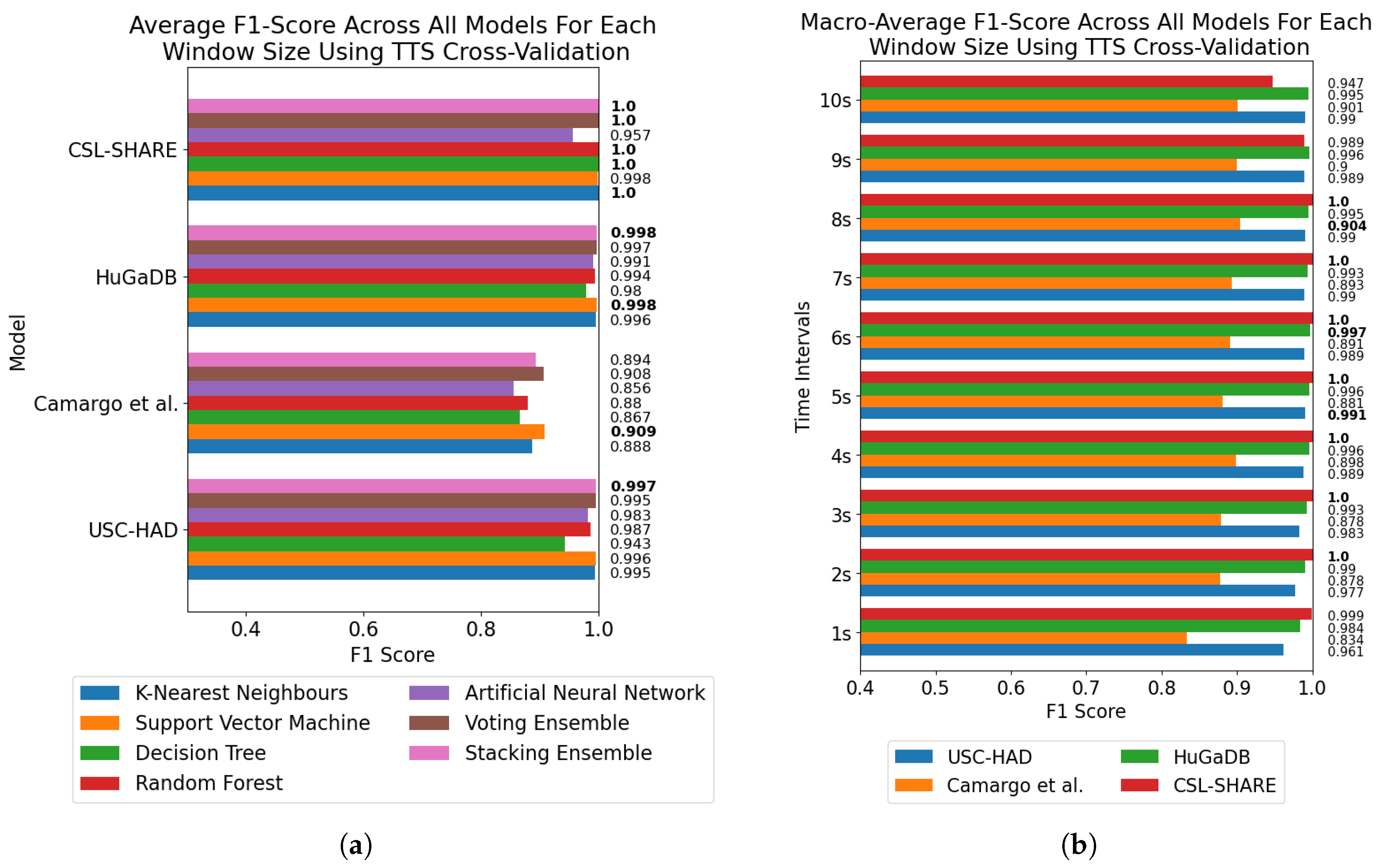
To assess the performance of each model, this study considered both macro-average accuracy and the F1-score. While macro-average accuracy provides a straightforward overview of a model by reporting the mean classification accuracy across all classes, it can be misleading in the presence of large class imbalances, as it does not account for differences in class distribution. To address this, the macro-average F1-score was also reported, which provides a more balanced measure of performance across classes. For each dataset, walking was the primary class, with around 10× more walking data than stair ascent and stair descent data. Standing data varied between datasets but were typically around 2–3× more numerous than data in the stair ascent and stair descent classes.
3. Results
To determine the optimal window size for sliding window feature extraction, each model was trained using the PCA-reduced feature set for each window size, ranging from 1 to 10 s. We selected 10 s as the maximum time due to issues with class distributions and the number of samples in each class at larger window sizes. This process was repeated three times for each model to reduce the impact of random initialisations, which can lead to models becoming stuck in local minima during training. The results for subject-dependent cross-validation can be seen in Figure 1, Figure 2, Figure 3 and Figure 4, whilst the results for subject-independent cross-validation can be found in Figure 5, Figure 6, Figure 7 and Figure 8. A full list of performance metrics for each dataset and window size can be found in Appendix A.
Figure 1.
Trend graphs showing the mean accuracy across all models and window sizes for the four datasets in this analysis when using TTS cross-validation. (a) USC-HAD. (b) Camargo et al. (c) HuGaDB. (d) CSL-SHARE.
Figure 2.
Trend graphs showing the mean F1-score across all models and window sizes for the four datasets in this analysis when using TTS cross-validation. (a) USC-HAD. (b) Camargo et al. (c) HuGaDB. (d) CSL-SHARE.
Figure 3.
Model and window size effect on classification accuracy across all four datasets using TTS cross-validation. The highest-performing model for each dataset and window size is marked in bold. (a) Average accuracy for each model across all window sizes for each dataset. (b) Average accuracy across all models at each window size from 1 to 10 s for each dataset.
Figure 4.
Model and window size effect on F1-score across all four datasets using TTS cross-validation. The highest-performing model for each dataset and window size is marked in bold. (a) Average F1-score for each model across all window sizes for each dataset. (b) Average F1-score across all models at each window size from 1 to 10 s for each dataset.
Figure 5.
Trend graphs showing the mean accuracy across all models and window sizes for the four datasets in this analysis when using LOSO cross-validation. (a) USC-HAD. (b) Camargo et al. (c) HuGaDB. (d) CSL-SHARE.

Figure 6.
Trend graphs showing the mean F1-score across all models and window sizes for the four datasets in this analysis when using LOSO cross-validation. (a) USC-HAD. (b) Camargo et al. (c) HuGaDB. (d) CSL-SHARE.
Figure 7.
Model and window size effect on classification accuracy across all four datasets using LOSO cross-validation. The highest-performing model for each dataset and window size is marked in bold. (a) Average accuracy for each model across all window sizes for each dataset. (b) Average accuracy across all models at each window size from 1 to 10 s for each dataset.
Figure 8.
Model and window size effect on F1-score across all four datasets using LOSO cross-validation. The highest-performing model for each dataset and window size is marked in bold. (a) Average F1-score for each model across all window sizes for each dataset. (b) Average F1-score across all models at each window size from 1 to 10 s for each dataset.
3.1. Subject-Dependent Cross-Validation
3.1.1. Determining Optimal Window Sizes
Figure 1 and Figure 2 show the mean performance of each model over the three repeat trials for each window size. The trend lines present in these figures demonstrate an increase in both accuracy and the F1-score with window size for subject-dependent cross-validation using TTS across all models and all datasets. The exceptions to this trend suggest that overfitting may have occurred as the number of samples decreased, with some models decreasing in performance with 9 and 10 s window sizes, where the number of data from each class was at a minimum. This issue was most prevalent with the ANNs among the smaller datasets, whilst the Camargo et al. dataset was the only one in which the ANN performance metrics did not drop at higher window size values. Although performance generally trended upwards with window size, all datasets except for CSL-SHARE, which exhibited 100% accuracy and a 100% F1-score for most models at all window sizes, plateaued at around 4–5 s. Furthermore, CSL-SHARE appeared to exhibit reduced performance at higher window sizes for both the ANN and SVM, likely due to a lack of data.
Figure 3 and Figure 4 show the average highest-performing model among all window sizes, along with the average accuracy and F1-score at each window size across all models. These figures highlight the SVM and the stacking ensemble classifier as the most capable models across all window sizes and that the best model performances occurred at window sizes of 4–8 s.
Regarding the individual (non-ensemble) highest-performing model, all models performed fairly similarly between datasets, with the SVM being the only model that performed significantly higher than others with average accuracies of 99.6%, 83.7%, 99.8%, and 100% and average F1-scores of 99.7%, 90.9%, 99.8%, and 100% on each of the USC-HAD, Camargo et al., HuGaDB, and CSL-SHARE datasets, respectively. However, these results also suggest there may be an issue with the Camargo et al. dataset, as the average accuracies for all models and window sizes were far more reduced for this dataset when compared with the others. An overview of the highest-performing individual models can be found in Table 3.
Table 3.
Maximum accuracy, precision, recall, and F1-Score for each dataset, non-ensemble model, and method of cross-validation.
3.1.2. Individual Sensor Analysis
The optimal window sizes for each dataset were used to determine the sensor importance for achieving high accuracies among the four core activities. As USC-HAD contained just a single sensor, it was excluded from this analysis. Due to its high performance across all datasets, and due to the SVM failing to converge on these reduced datasets, an ANN was trained to classify between the four activities using data from individual sensors.
Table 4, Table 5 and Table 6 show the precision, recall, F1-score, and accuracy of the ANN trained from features extracted from each sensor in the Camargo et al., HuGaDB, and CSL-SHARE datasets, respectively. These tables highlight IMUs as the most effective individual sensors, exhibiting accuracies of 87.4–100% and F1-scores of 74.4–100% across all datasets. Goniometers also appear as high-performing sensors, with the three-axis goniometers at the hip and ankle in the Camargo et al. dataset exhibiting performance metrics marginally lower than those of the IMUs, with accuracies of 86.8% and 87.4% and F1-scores of 74.2% and 70.8%, respectively. Following the three-axis goniometers, both the Camargo et al. and CSL-SHARE datasets feature two-axis goniometers at the knee, which enabled accuracies of 74.2% and 99.6%, respectively. However, with an F1-score of just 44.5% for the Camargo et al. knee goniometer, this may suggest that two-axis goniometers lacked the data dimensionality for high-accuracy HAR. Finally, the EMG sensors exhibited the lowest performance metrics across all datasets. Among the EMG sensors, placement heavily affected classification accuracy, with the vastus lateralis and biceps femoris performing extremely poorly, whilst the tibialis anterior, soleus, gastrocnemius, and vastus medialis generally outperformed EMG sensors placed on other muscles. However, even the highest-performing EMG sensors in each dataset exhibit F1-scores significantly lower than those of the IMUs.
Table 4.
Subject-dependent performance metrics of each individual sensor in the Camargo et al. dataset.
Table 5.
Subject-dependent performance metrics of each individual sensor in the HuGaDB dataset.
Table 6.
Subject-dependent performance metrics of each individual sensor in the CSL-SHARE dataset.
3.2. Subject-Independent Cross-Validation
3.2.1. Determining Optimal Window Sizes
Figure 5 shows the performance trends of each model at each window size for the four datasets in this study using LOSO cross-validation. The maximum accuracy for USC-HAD occurred at a 10 s window size with the SVM exhibiting an accuracy of 91.9% and an F1-score of 81.2%, whilst the Camargo et al. dataset achieved a maximum accuracy of 80.8% and an F1-score of 85.2% at 9 s using the ANN. Both the CSL-SHARE and HuGaDB datasets achieved a 100% classification accuracy and an F1-score with multiple model types at 1 and 2 s, respectively, which was maintained up to a window size of 10 s. The DT, RF, and KNN models performed erratically across all datasets and window sizes, which caused the stacking and voting ensemble methods to underperform when compared to the ANN and SVM.
Figure 7 shows the mean accuracies across all time windows and models. From Figure 7a, the SVMs and ANNs appear as the classifiers with the highest classification accuracy where there is a statistically significant difference between classifier performances, with the SVMs achieving 79.1%, 68.4%, 98.8%, and 99.9% accuracies and F1-scores of 66.9%, 66.1%, 99.2%, and 100%, whilst the ANNs achieved 75.4%, 73.6%, 99.9%, and 100% accuracies and F1-scores of 66.3%, 76.7%, 99.9% and 100% on each of the USC-HAD, Camargo et al., HuGaDB, and CSL-SHARE datasets, respectively. As such, the ANN and SVM can clearly be identified as the highest-performing model types across all datasets, as seen in Table 3. Concerning window size, each dataset presented a different window size at which the maximum mean accuracy occurred. For USC-HAD, the highest mean accuracy and F1-score across all models occurred at 2–3 s window sizes, whilst for the Camargo et al. dataset, these occurred at 5 s, both of which were similar to the time at which model accuracy plateaued using subject-dependent cross-validation. Both HuGaDB and CSL-SHARE achieved accuracies of 100% with several models, but due to the lower accuracies with other models, their highest mean performances occurred at 8 s for HuGaDB and any value from 3 to 10 s for CSL-SHARE.
3.2.2. Individual Sensor Analysis
As with the subject-dependent individual sensor analysis, the ANN was trained on the features extracted from each individual sensor. Table 7, Table 8 and Table 9 show the performance metrics for each sensor used in the Camargo et al., HuGaDB, and CSL-SHARE datasets, respectively. Like with the subject-dependent analysis, the IMUs achieved the highest accuracies across two of the three datasets, whilst the EMG sensors exhibited consistently poor performances. In this scenario, performance metrics were generally reduced, with only the EMG sensors placed on the gastrocnemius medialis and gluteus medius for the Camargo et al. dataset and the vastus medialis for the CSL-SHARE dataset achieving accuracies and F1-scores above 50%. The three-axis goniometers on the hip from the Camargo et al. dataset exhibited higher performance metrics than the IMUs in this case, with the ankle goniometer outperforming all but the foot IMU, whilst the two-axis goniometers positioned on the knee in the Camargo et al. and CSL-SHARE datasets exhibited much lower performance metrics.
Table 7.
Subject-independent performance metrics of each individual sensor in the Camargo et al. dataset.
Table 8.
Subject-independent performance metrics of each individual sensor in the HuGaDB dataset.
Table 9.
Subject-independent performance metrics of each individual sensor in the CSL-SHARE dataset.
Overall, the trends among these sensors were largely the same as with the subject-dependent analysis, with the main difference being the high performance of the three-axis goniometers, along with an overall reduction in accuracy for the two-axis goniometers and EMG sensors, further highlighting the volatility of performance when using these sensors.
4. Discussions
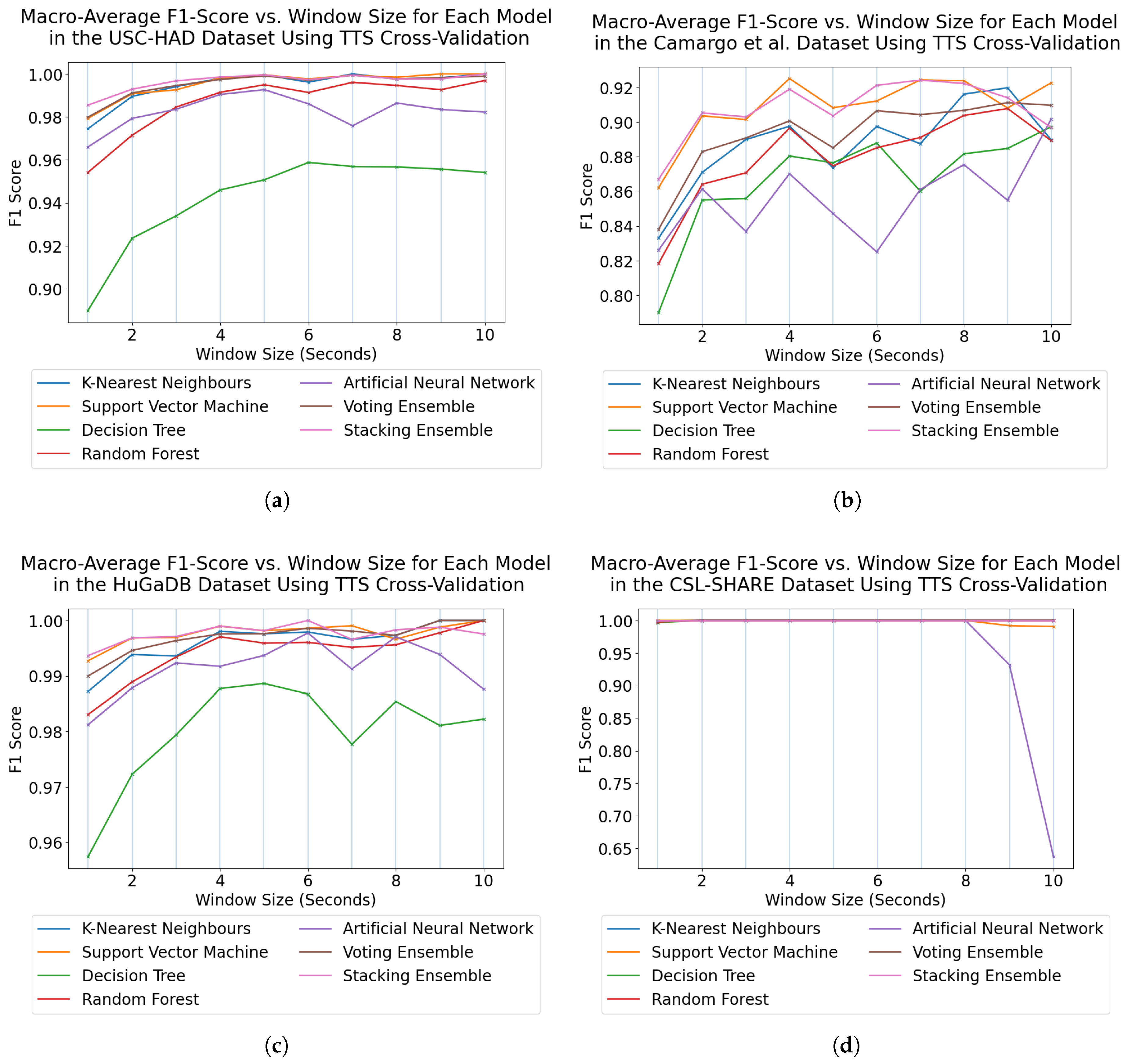
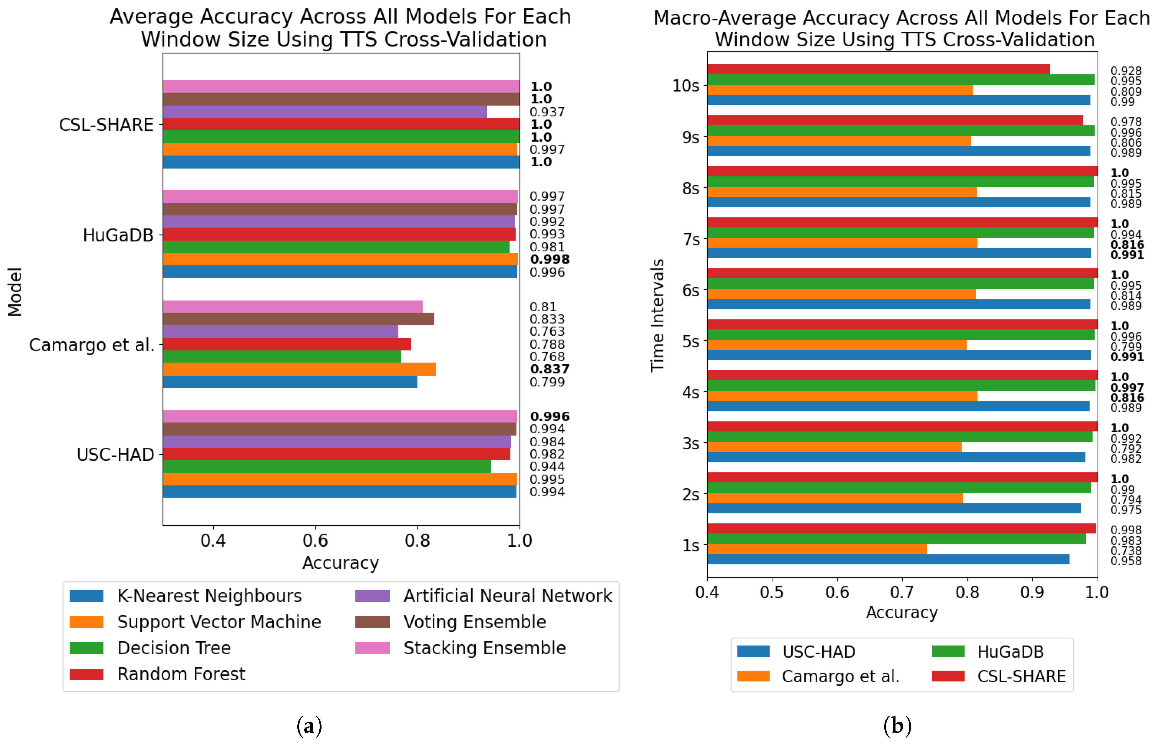
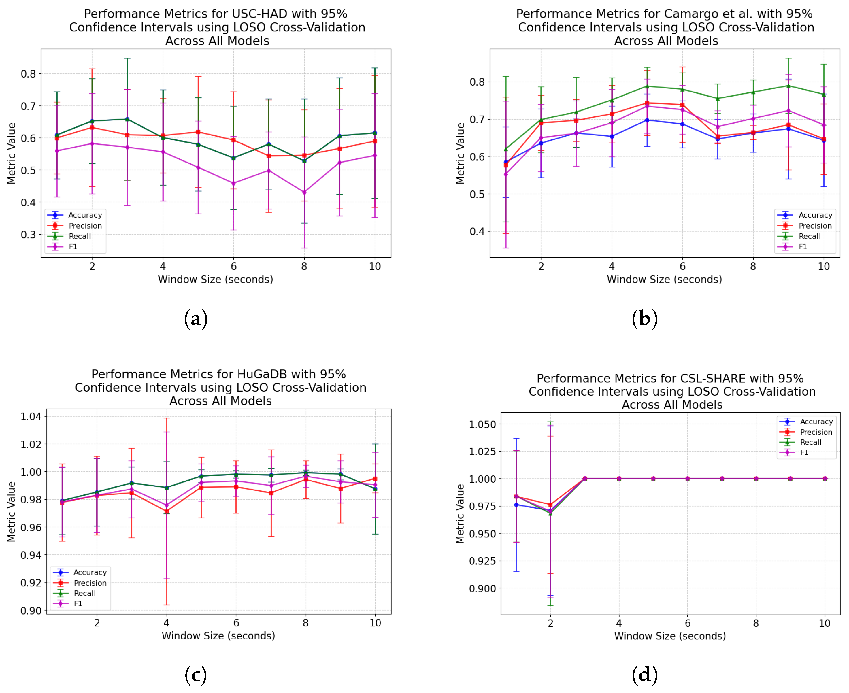
The results of the window size analysis did not exhibit a consistent peak or plateau, with accuracies appearing volatile across the four datasets for each window size and trend lines displaying misaligned peaks. Furthermore, the averaging of accuracies across all models at each window size showed no clear single optimal window size across the four datasets and methods of cross-validation.
It must be noted that the performance metrics of the Camargo et al. dataset did not align with the other multimodal datasets in terms of overall classification accuracy. These systems all made use of the same six-axis IMU positioned on the thigh, yet the Camargo et al. dataset achieved significantly reduced accuracies when trained on only this sensor when compared to HuGaDB and CSL-SHARE. Given the large number of controlled variables in this study, this indicates a difference in experimental procedure or activity data distribution, which negatively affects the results of the Camargo et al. dataset. 
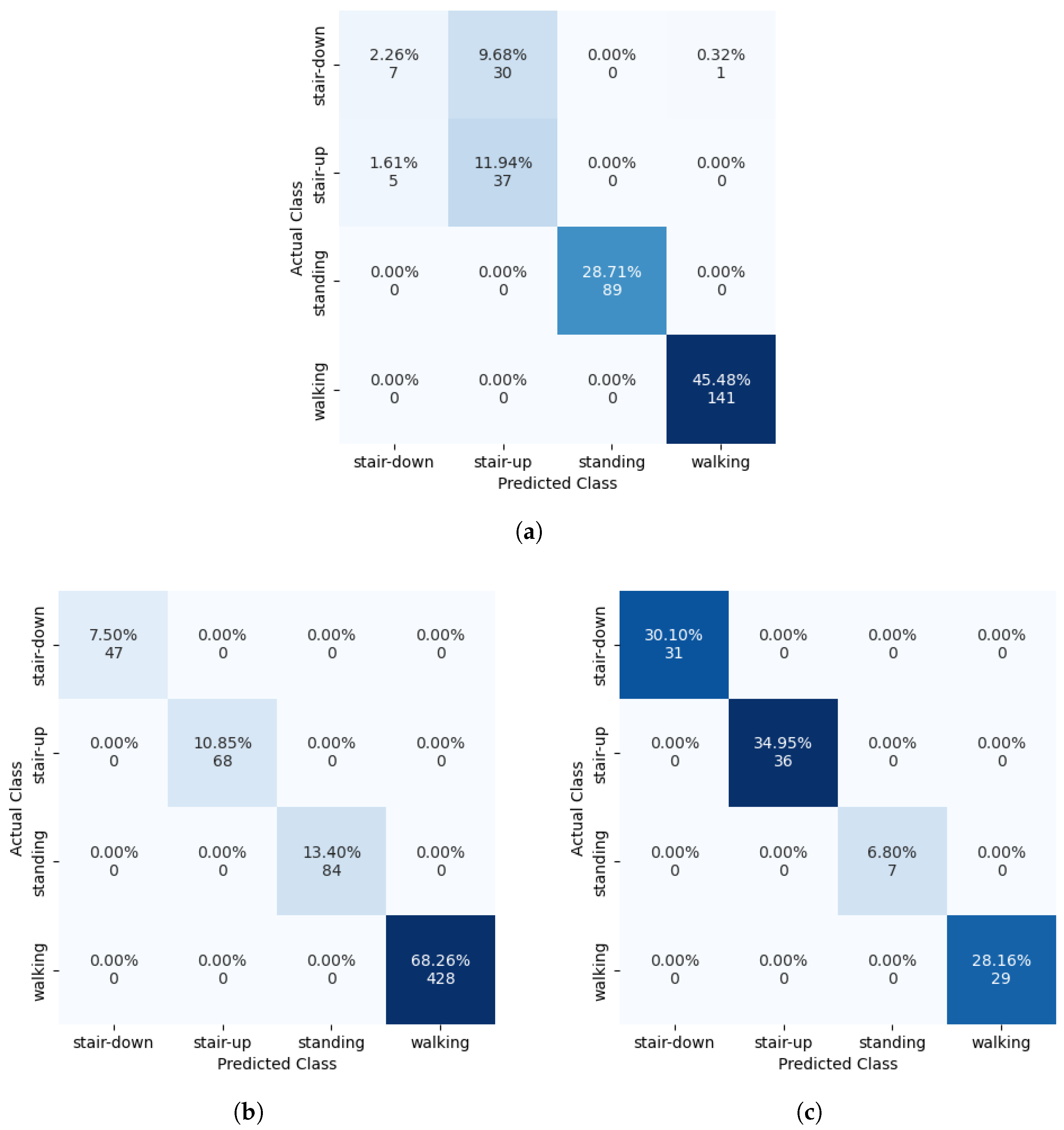
Figure 9a shows the confusion matrix for an SVM trained on the Camargo et al. dataset, which shows that the misclassifications are between the stair ascend and stair descend classes. This is also shown not to be caused by sample weighting, as Figure 9b,c show the confusion matrices for the HuGaDB and CSL-SHARE datasets, respectively, which feature more extreme sample weightings than the Camargo et al. dataset whilst achieving 100% accuracy.
Figure 9.
Confusion matrices of an SVM trained on data from a single EMG sensor using LOSO cross-validation. (a) Camargo et al. Vastus Lateralis. (b) HuGaDB Vastus Lateralis. (c) CSL-SHARE Vastus Medialis EMG.
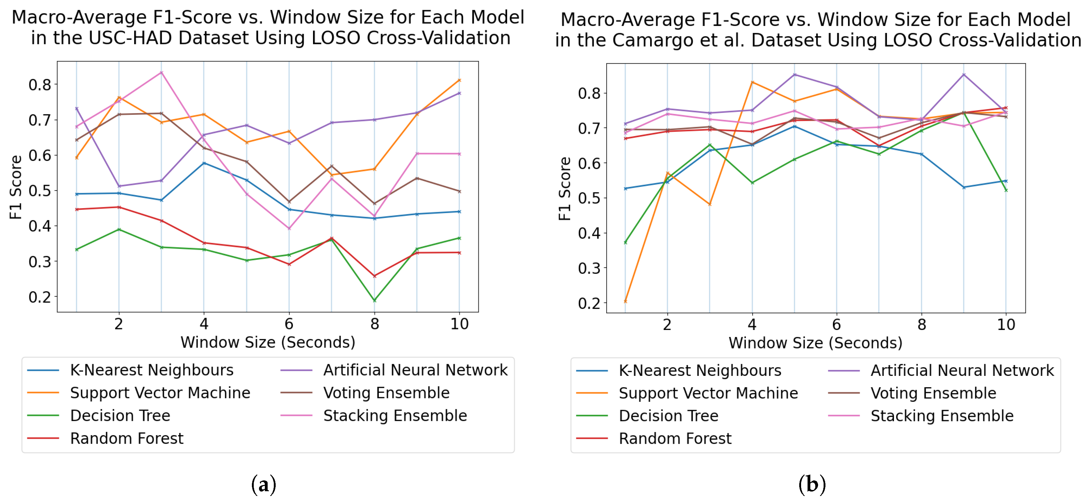
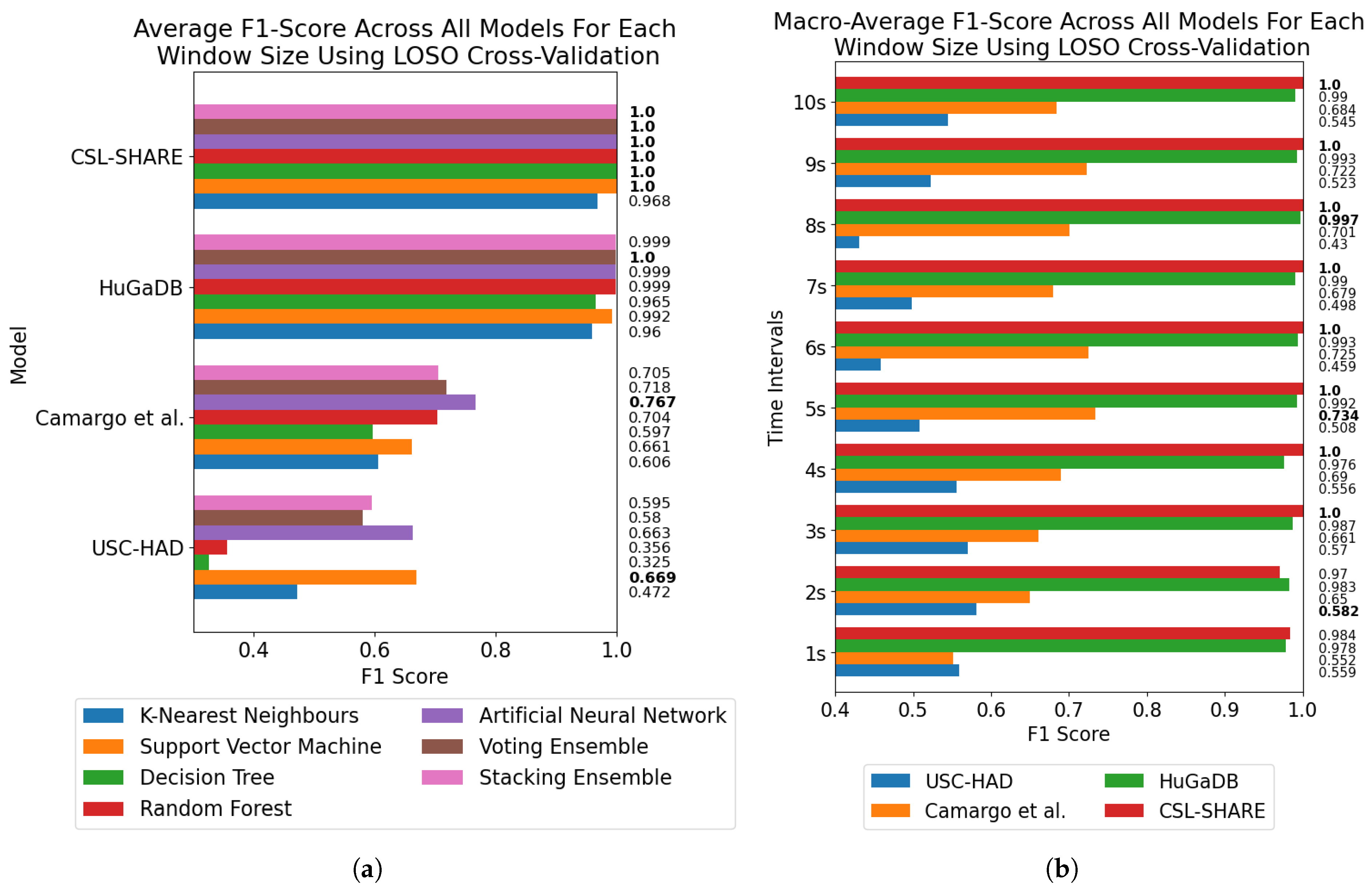
Figure 9 highlights SVMs as the most effective individual models for HAR using subject-dependent cross-validation, with ANNs proving more effective when using subject-independent cross-validation. This is likely due to the tendency for ANNs to overfit, which was further pronounced by the use of a TTS in creating test data for subject-dependent cross-validation, whereas SVMs typically perform well in these scenarios due to the maximisation of the margin when creating a decision boundary.
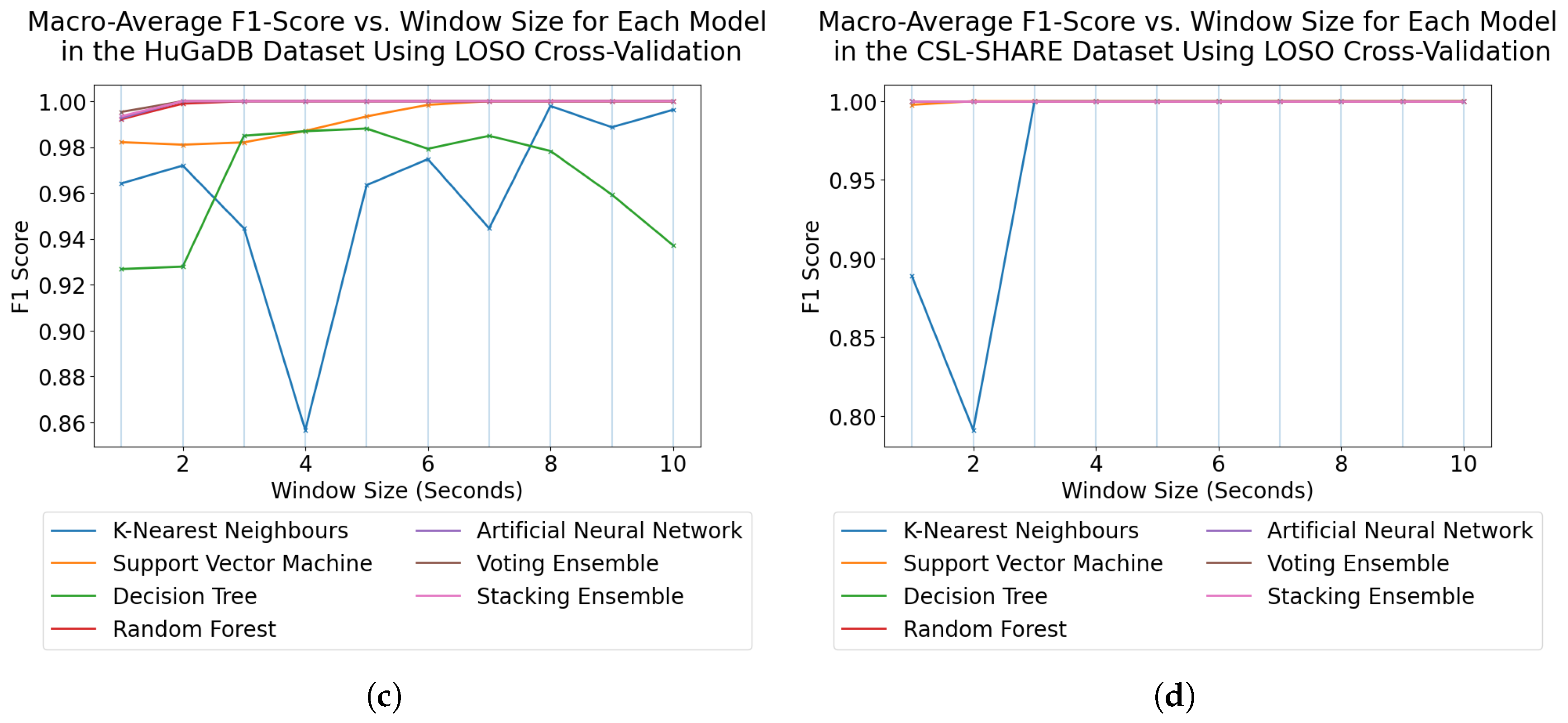
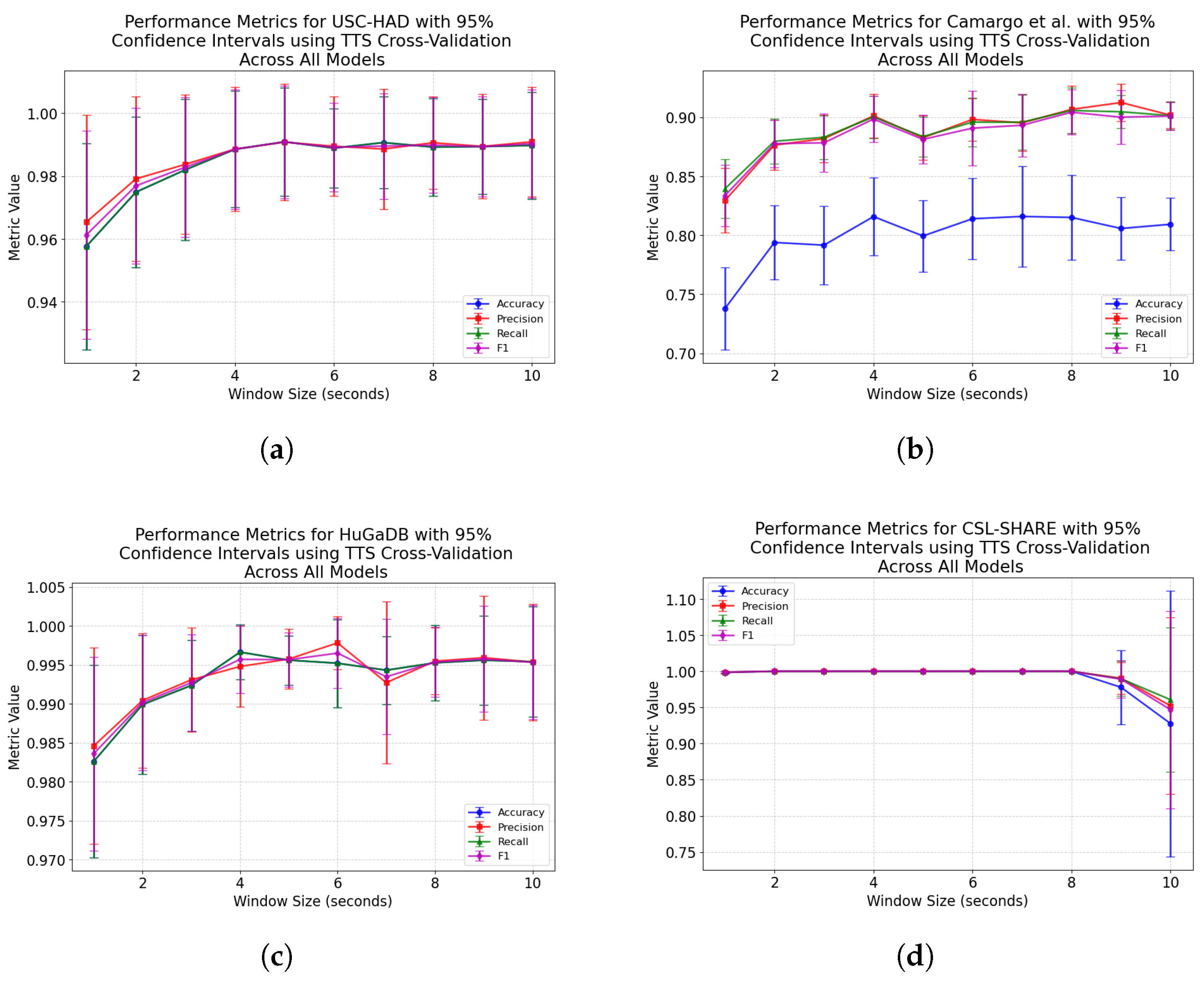
For subject-dependent cross-validation, peak accuracies occurred at smaller window sizes, ranging from 2–5 s. The trend lines in Figure 1 and Figure 5 also exhibit rises in accuracy for some models as they approach a 10-s window size, indicating that, if the dataset contains enough samples in each class for this to be viable, larger window sizes offer richer features which lead to higher classification accuracies. For subject-independent cross-validation, the highest-performing model accuracies occurred at 2, 3, 5, and 10 s for the HuGaDB, CSL-SHARE, Camargo et al., and USC-HAD datasets, respectively. Apart from USC-HAD, this further highlights the range of 2–5 s as an effective range of window sizes in achieving high classification accuracy for the core activities of HAR.
Aside from the Camargo et al. dataset, the multimodal datasets achieved much higher classification accuracies when using the same models and window sizes, which allowed high accuracies to be obtained with much smaller window sizes. This has significant implications when considering the delay time, portability, and convenience of systems, as increasing the number of sensors can enable high-accuracy HAR using very computationally inexpensive methods such as DT. These computationally low-cost methods can also allow designers of real-time HAR systems to incorporate low-power computational devices with reduced size profiles and battery consumption, therefore increasing the comfort and convenience of the devices. Additionally, the fact that high accuracies can be obtained in multimodal systems with low window sizes means that much faster response times can be achieved for real-time HAR systems, as some models trained on the CSL-SHARE dataset achieved 100% accuracy using just 1 s windows with a 0.25 s fixed delay time caused by the step size. Whilst it was shown that accuracy at each window size was dependent on the sensor types used in each dataset, further work is needed to identify how model performance varies with window size for each individual sensor type. This will enable the building of a knowledge database to help future researchers choose a window size given a sensor system without the need for lengthy, brute-force approaches to finding the most appropriate window size, combination of sensors, and choice of model for each novel dataset produced in this field.
Regarding individual sensor types, the IMUs and three-axis goniometers generally exhibited the highest accuracies, followed by the two-axis goniometers and finally the EMG sensors. Among IMU locations, accuracy varied among the different locations, with no clear ranking between all datasets. Only the Camargo et al. and CSL-SHARE datasets featured goniometers, with the three-axis goniometers at the thigh and ankle in the Camargo et al. dataset showing large performance improvements over the two-axis goniometers located on the knee in both the Camargo et al. and CSL-SHARE datasets. Goniometers are low-power devices with fewer data dimensions than IMUs which can be incorporated into smart clothing devices to improve comfort and convenience. Given the competitive performance of goniometers in this study, three-axis goniometers should be considered in future datasets and HAR systems. On the other hand, EMG sensor performance was volatile between locations and datasets, which may be due to differences in filtering methods, varying placements on muscles, or changes in experimental procedures. As such, it is not currently possible to compare the locations of these sensors, particularly with so few datasets for reference. More datasets are required to accurately rank the locations of these sensors so that the impact of differences in experimental setup can be minimised.
Regarding the sample rates of each dataset, no correlation was present between the native sample rates of each dataset and the final classification accuracy, with the HuGaDB dataset exhibiting far higher accuracies than USC-HAD and the Camargo et al. dataset, despite having the lowest native sample rate of 60 Hz. As such, whilst sample rate is expected to have an effect at even lower values, 60 Hz can be considered a sufficient sample rate for high-accuracy HAR.
These results align with the findings of Banos et al. [23], who found that increased window size does not necessarily increase activity classification performance across many datasets. However, our study also offers insight into the reason for this assumption, with subject-dependent cross-validation demonstrating this pattern until accuracy and F1-score began to reduce at larger window size values due to insufficient sample sizes. Crucially, this work considers both subject-dependent and subject-independent methods of cross-validation, which highlights how the choice of cross-validation method impacts the selection of an optimal window size, which was not considered in the study [23]. Niazi et al. [25] considered the effect of window size and sample rate on classification accuracy using an RF classifier, where it was reported that window sizes could appear optimal between 2–10 s using subject-dependent cross-validation. Our results support these findings and demonstrate that this also applies to additional classical Machine Learning models such as the ANN, SVM, KNN, and DT. Duan et al. [28] considered the optimal placement of sensors using deep learning techniques for a single dataset, finding that sensors placed on the right leg exhibited increased performance. Our results align with the findings of this study, with the HuGaDB dataset demonstrating that, when subject-independent cross-validation was used, the performance metrics of the right leg were higher than those of the left. Finally, Khan et al. [30] report that sensor performance is dependent on the activities being performed in the dataset. By removing the variation between datasets, our study controlled for this factor, resulting in a reliable ranking of sensor locations that achieved high performances and offer future researchers the information necessary to build effective HAR systems.
Finally, this study featured several limitations due to the computational cost of performing this analysis. The first of these limitations was the lack of investigation into the effects of window step size, which was set to 25% of the total window size. This could have been set to a fixed time value for all window sizes or have been individually analysed to explore the co-dependent effects of step size and window size. Furthermore, the availability of datasets which feature a sufficiently large number of participants and sensors, along with the core activities included in this study, was limited, resulting in the inclusion of just four datasets.
5. Conclusions and Future Work
This study is the first of its kind in providing a bias-reduced, normalised, cross-dataset analysis to determine and rank the highest-performing sensor types for Human Activity Recognition. First, ANNs were found to be the highest-performing models across multiple multimodal HAR datasets, closely followed by SVMs, with the optimal window size being in the range of 2–5 s when using the semi-non-overlapping sliding window approach to feature engineering with a 75% overlap. Where datasets were large enough to reduce the impact of class imbalance, or models were sufficiently powerful to generalise with smaller sample numbers, accuracies were also shown to trend upwards with larger window sizes of 9–10 s. Regarding the contributions of individual sensor types to classification accuracy, IMUs placed on the thigh and three-axis goniometers on the thigh and ankle were the overall largest contributors to high-accuracy HAR, whilst EMG sensors were found to exhibit volatile accuracies which was likely due to the difficulty in ensuring that the sensors were in the same place and calibrated equally for different subjects. It remains appropriate for researchers to collect large HAR datasets and to investigate alternative methods of HAR using multimodal sensor systems and smart clothing to investigate how the size and inconvenience of these systems can be minimised whilst maintaining high accuracy using low-computational-complexity classification methods.
This study was limited by the scarcity of open multimodal gait datasets with large numbers of sensors and common activities. As a result, future work in this area should consider more datasets, activities (including fall-related activities), and sensor types to investigate how classifier performance in HAR is affected by these properties. Additionally, elements such as step size, the proportion of data for each activity, and time-series features should be investigated for their contribution towards achieving efficient and convenient high-accuracy HAR. Finally, the time and space complexity of these algorithms should be considered under the various window sizes to evaluate the feasibility of deploying these optimised models in real-world HAR applications.
Author Contributions
Conceptualisation, J.C.M., A.A.D.-S., S.Q.X., R.J.O.; methodology, J.C.M.; software, J.C.M.; validation, J.C.M.; formal analysis, J.C.M.; investigation, J.C.M.; resources, J.C.M.; data curation, J.C.M.; writing—original draft preparation, J.C.M.; writing—review and editing, A.A.D.-S., S.Q.X., R.J.O.; visualisation, J.C.M.; supervision, A.A.D.-S., S.Q.X., R.J.O.; project administration, A.A.D.-S., S.Q.X., R.J.O.; funding acquisition, A.A.D.-S. All authors have read and agreed to the published version of the manuscript.
Funding
This research was funded by the United Kingdom Research and Innovation (UKRI)—Engineering and Physical Sciences Research Council (EPSRC) (grant number EP/T517860/1).
Institutional Review Board Statement
Not applicable.
Informed Consent Statement
Not applicable.
Data Availability Statement
Data are contained within the article and available upon request by contacting the authors.
Conflicts of Interest
The authors declare no conflicts of interest.
Abbreviations
The following abbreviations are used in this manuscript:
| ANN | Artificial Neural Network |
| DT | Decision Tree |
| EMG | Electromyography |
| HAR | Human Activity Recognition |
| IMU | Inertial Measurement Unit |
| IoT | Internet of Things |
| KNN | K-Nearest Neighbors |
| LOSO | Leave-One-Subject-Out |
| ML | Machine Learning |
| PCA | Principal Component Analysis |
| RF | Random Forest |
| SVM | Support Vector Machine |
| TTS | Train–Test Split |
Appendix A
Figure A1 and Figure A2 along with Table A1, Table A2, Table A3, Table A4, Table A5, Table A6, Table A7 and Table A8 show the performance metrics of each dataset and method of cross-validation, including the mean, standard deviation, and 95% confidence intervals.
Figure A1.
Trend graphs showing the macro-averaged performance metrics across all models and window sizes for the four datasets in this analysis when using TTS cross-validation. (a) USC-HAD. (b) Camargo et al. (c) HuGaDB. (d) CSL-SHARE.
Figure A2.
Trend graphs showing the macro-averaged performance metrics across all models and window sizes for the four datasets in this analysis when using TTS cross-validation. (a) USC-HAD. (b) Camargo et al. (c) HuGaDB. (d) CSL-SHARE.
Table A1.
Performance metrics for the USC HAD dataset using TTS cross-validation with 95% confidence intervals.
Table A1.
Performance metrics for the USC HAD dataset using TTS cross-validation with 95% confidence intervals.
| Window (s) | Metric | Mean | Std | CI Low | CI High |
|---|---|---|---|---|---|
| 1 | Accuracy | 0.9577 | 0.0328 | 0.9273 | 0.9881 |
| Precision | 0.9654 | 0.0341 | 0.9339 | 0.9970 | |
| Recall | 0.9577 | 0.0328 | 0.9273 | 0.9881 | |
| F1-score | 0.9613 | 0.0332 | 0.9306 | 0.9920 | |
| 2 | Accuracy | 0.9749 | 0.0240 | 0.9527 | 0.9971 |
| Precision | 0.9791 | 0.0262 | 0.9549 | 1.0034 | |
| Recall | 0.9749 | 0.0240 | 0.9527 | 0.9971 | |
| F1-score | 0.9769 | 0.0248 | 0.9540 | 0.9999 | |
| 3 | Accuracy | 0.9820 | 0.0224 | 0.9613 | 1.0027 |
| Precision | 0.9838 | 0.0221 | 0.9633 | 1.0043 | |
| Recall | 0.9820 | 0.0224 | 0.9613 | 1.0027 | |
| F1-score | 0.9829 | 0.0222 | 0.9624 | 1.0034 | |
| 4 | Accuracy | 0.9885 | 0.0185 | 0.9714 | 1.0057 |
| Precision | 0.9886 | 0.0197 | 0.9704 | 1.0068 | |
| Recall | 0.9885 | 0.0185 | 0.9714 | 1.0057 | |
| F1-score | 0.9886 | 0.0191 | 0.9709 | 1.0062 | |
| 5 | Accuracy | 0.9910 | 0.0172 | 0.9750 | 1.0069 |
| Precision | 0.9908 | 0.0186 | 0.9736 | 1.0080 | |
| Recall | 0.9910 | 0.0172 | 0.9750 | 1.0069 | |
| F1-score | 0.9909 | 0.0179 | 0.9743 | 1.0074 | |
| 6 | Accuracy | 0.9889 | 0.0126 | 0.9773 | 1.0005 |
| Precision | 0.9895 | 0.0158 | 0.9750 | 1.0041 | |
| Recall | 0.9889 | 0.0126 | 0.9773 | 1.0005 | |
| F1-score | 0.9892 | 0.0140 | 0.9762 | 1.0022 | |
| 7 | Accuracy | 0.9907 | 0.0146 | 0.9772 | 1.0042 |
| Precision | 0.9886 | 0.0191 | 0.9710 | 1.0063 | |
| Recall | 0.9907 | 0.0146 | 0.9772 | 1.0042 | |
| F1-score | 0.9896 | 0.0168 | 0.9740 | 1.0051 | |
| 8 | Accuracy | 0.9893 | 0.0155 | 0.9749 | 1.0036 |
| Precision | 0.9906 | 0.0147 | 0.9771 | 1.0042 | |
| Recall | 0.9893 | 0.0155 | 0.9749 | 1.0036 | |
| F1-score | 0.9899 | 0.0152 | 0.9758 | 1.0040 | |
| 9 | Accuracy | 0.9894 | 0.0152 | 0.9754 | 1.0035 |
| Precision | 0.9895 | 0.0166 | 0.9741 | 1.0049 | |
| Recall | 0.9894 | 0.0152 | 0.9754 | 1.0035 | |
| F1-score | 0.9894 | 0.0159 | 0.9747 | 1.0041 | |
| 10 | Accuracy | 0.9898 | 0.0170 | 0.9741 | 1.0055 |
| Precision | 0.9909 | 0.0174 | 0.9749 | 1.0070 | |
| Recall | 0.9898 | 0.0170 | 0.9741 | 1.0055 | |
| F1-score | 0.9903 | 0.0172 | 0.9744 | 1.0062 |
Table A2.
Performance metrics for the USC HAD dataset using LOSO cross-validation with 95% confidence intervals.
Table A2.
Performance metrics for the USC HAD dataset using LOSO cross-validation with 95% confidence intervals.
| Window (s) | Metric | Mean | Std | CI Low | CI High |
|---|---|---|---|---|---|
| 1 | Accuracy | 0.6083 | 0.1353 | 0.4831 | 0.7334 |
| Precision | 0.5992 | 0.1117 | 0.4959 | 0.7025 | |
| Recall | 0.6083 | 0.1353 | 0.4831 | 0.7334 | |
| F1-score | 0.5589 | 0.1424 | 0.4272 | 0.6907 | |
| 2 | Accuracy | 0.6521 | 0.1317 | 0.5303 | 0.7739 |
| Precision | 0.6319 | 0.1831 | 0.4626 | 0.8012 | |
| Recall | 0.6521 | 0.1317 | 0.5303 | 0.7739 | |
| F1-score | 0.5817 | 0.1563 | 0.4372 | 0.7262 | |
| 3 | Accuracy | 0.6579 | 0.1900 | 0.4821 | 0.8336 |
| Precision | 0.6092 | 0.1416 | 0.4783 | 0.7402 | |
| Recall | 0.6579 | 0.1900 | 0.4821 | 0.8336 | |
| F1-score | 0.5705 | 0.1804 | 0.4036 | 0.7373 | |
| 4 | Accuracy | 0.6004 | 0.1481 | 0.4635 | 0.7374 |
| Precision | 0.6065 | 0.1163 | 0.4990 | 0.7141 | |
| Recall | 0.6004 | 0.1481 | 0.4635 | 0.7374 | |
| F1-score | 0.5561 | 0.1524 | 0.4152 | 0.6970 | |
| 5 | Accuracy | 0.5795 | 0.1451 | 0.4453 | 0.7137 |
| Precision | 0.6181 | 0.1726 | 0.4584 | 0.7777 | |
| Recall | 0.5795 | 0.1451 | 0.4453 | 0.7137 | |
| F1-score | 0.5079 | 0.1443 | 0.3745 | 0.6414 | |
| 6 | Accuracy | 0.5372 | 0.1601 | 0.3891 | 0.6852 |
| Precision | 0.5928 | 0.1511 | 0.4530 | 0.7326 | |
| Recall | 0.5372 | 0.1601 | 0.3891 | 0.6852 | |
| F1-score | 0.4586 | 0.1453 | 0.3241 | 0.5930 | |
| 7 | Accuracy | 0.5799 | 0.1415 | 0.4490 | 0.7108 |
| Precision | 0.5434 | 0.1746 | 0.3819 | 0.7049 | |
| Recall | 0.5799 | 0.1415 | 0.4490 | 0.7108 | |
| F1-score | 0.4982 | 0.1205 | 0.3868 | 0.6096 | |
| 8 | Accuracy | 0.5279 | 0.1938 | 0.3486 | 0.7071 |
| Precision | 0.5455 | 0.1416 | 0.4145 | 0.6764 | |
| Recall | 0.5279 | 0.1938 | 0.3486 | 0.7071 | |
| F1-score | 0.4304 | 0.1727 | 0.2706 | 0.5901 | |
| 9 | Accuracy | 0.6061 | 0.1817 | 0.4380 | 0.7741 |
| Precision | 0.5663 | 0.1864 | 0.3939 | 0.7387 | |
| Recall | 0.6061 | 0.1817 | 0.4380 | 0.7741 | |
| F1-score | 0.5227 | 0.1661 | 0.3691 | 0.6764 | |
| 10 | Accuracy | 0.6150 | 0.2031 | 0.4271 | 0.8028 |
| Precision | 0.5895 | 0.2052 | 0.3997 | 0.7793 | |
| Recall | 0.6150 | 0.2031 | 0.4271 | 0.8028 | |
| F1-score | 0.5448 | 0.1925 | 0.3668 | 0.7228 |
Table A3.
Performance metrics for the CSL-SHARE dataset using TTS cross-validation with 95% confidence intervals.
Table A3.
Performance metrics for the CSL-SHARE dataset using TTS cross-validation with 95% confidence intervals.
| Window (s) | Metric | Mean | Std | CI Low | CI High |
|---|---|---|---|---|---|
| 1 | Accuracy | 0.9984 | 0.0015 | 0.9970 | 0.9998 |
| Precision | 0.9988 | 0.0012 | 0.9977 | 0.9999 | |
| Recall | 0.9988 | 0.0012 | 0.9977 | 0.9999 | |
| F1-score | 0.9988 | 0.0012 | 0.9977 | 0.9999 | |
| 2 | Accuracy | 1.0000 | 0.0000 | N/A | N/A |
| Precision | 1.0000 | 0.0000 | N/A | N/A | |
| Recall | 1.0000 | 0.0000 | N/A | N/A | |
| F1-score | 1.0000 | 0.0000 | N/A | N/A | |
| 3 | Accuracy | 1.0000 | 0.0000 | N/A | N/A |
| Precision | 1.0000 | 0.0000 | N/A | N/A | |
| Recall | 1.0000 | 0.0000 | N/A | N/A | |
| F1-score | 1.0000 | 0.0000 | N/A | N/A | |
| 4 | Accuracy | 1.0000 | 0.0000 | N/A | N/A |
| Precision | 1.0000 | 0.0000 | N/A | N/A | |
| Recall | 1.0000 | 0.0000 | N/A | N/A | |
| F1-score | 1.0000 | 0.0000 | N/A | N/A | |
| 5 | Accuracy | 1.0000 | 0.0000 | N/A | N/A |
| Precision | 1.0000 | 0.0000 | N/A | N/A | |
| Recall | 1.0000 | 0.0000 | N/A | N/A | |
| F1-score | 1.0000 | 0.0000 | N/A | N/A | |
| 6 | Accuracy | 1.0000 | 0.0000 | N/A | N/A |
| Precision | 1.0000 | 0.0000 | N/A | N/A | |
| Recall | 1.0000 | 0.0000 | N/A | N/A | |
| F1-score | 1.0000 | 0.0000 | N/A | N/A | |
| 7 | Accuracy | 1.0000 | 0.0000 | N/A | N/A |
| Precision | 1.0000 | 0.0000 | N/A | N/A | |
| Recall | 1.0000 | 0.0000 | N/A | N/A | |
| F1-score | 1.0000 | 0.0000 | N/A | N/A | |
| 8 | Accuracy | 1.0000 | 0.0000 | N/A | N/A |
| Precision | 1.0000 | 0.0000 | N/A | N/A | |
| Recall | 1.0000 | 0.0000 | N/A | N/A | |
| F1-score | 1.0000 | 0.0000 | N/A | N/A | |
| 9 | Accuracy | 0.9778 | 0.0514 | 0.9302 | 1.0254 |
| Precision | 0.9904 | 0.0222 | 0.9698 | 1.0109 | |
| Recall | 0.9896 | 0.0241 | 0.9674 | 1.0119 | |
| F1-score | 0.9891 | 0.0255 | 0.9655 | 1.0127 | |
| 10 | Accuracy | 0.9277 | 0.1839 | 0.7576 | 1.0977 |
| Precision | 0.9523 | 0.1223 | 0.8391 | 1.0654 | |
| Recall | 0.9607 | 0.1000 | 0.8682 | 1.0532 | |
| F1-score | 0.9469 | 0.1366 | 0.8206 | 1.0732 |
Table A4.
Performance metrics for the CSL-SHARE dataset using LOSO cross-validation with 95% confidence intervals.
Table A4.
Performance metrics for the CSL-SHARE dataset using LOSO cross-validation with 95% confidence intervals.
| Window (s) | Metric | Mean | Std | CI Low | CI High |
|---|---|---|---|---|---|
| 1 | Accuracy | 0.9762 | 0.0609 | 0.9199 | 1.0325 |
| Precision | 0.9837 | 0.0421 | 0.9448 | 1.0227 | |
| Recall | 0.9841 | 0.0412 | 0.9460 | 1.0222 | |
| F1-score | 0.9838 | 0.0419 | 0.9451 | 1.0225 | |
| 2 | Accuracy | 0.9708 | 0.0773 | 0.8993 | 1.0423 |
| Precision | 0.9762 | 0.0629 | 0.9181 | 1.0344 | |
| Recall | 0.9683 | 0.0840 | 0.8906 | 1.0459 | |
| F1-score | 0.9701 | 0.0790 | 0.8971 | 1.0432 | |
| 3 | Accuracy | 1.0000 | 0.0000 | N/A | N/A |
| Precision | 1.0000 | 0.0000 | N/A | N/A | |
| Recall | 1.0000 | 0.0000 | N/A | N/A | |
| F1-score | 1.0000 | 0.0000 | N/A | N/A | |
| 4 | Accuracy | 1.0000 | 0.0000 | N/A | N/A |
| Precision | 1.0000 | 0.0000 | N/A | N/A | |
| Recall | 1.0000 | 0.0000 | N/A | N/A | |
| F1-score | 1.0000 | 0.0000 | N/A | N/A | |
| 5 | Accuracy | 1.0000 | 0.0000 | N/A | N/A |
| Precision | 1.0000 | 0.0000 | N/A | N/A | |
| Recall | 1.0000 | 0.0000 | N/A | N/A | |
| F1-score | 1.0000 | 0.0000 | N/A | N/A | |
| 6 | Accuracy | 1.0000 | 0.0000 | N/A | N/A |
| Precision | 1.0000 | 0.0000 | N/A | N/A | |
| Recall | 1.0000 | 0.0000 | N/A | N/A | |
| F1-score | 1.0000 | 0.0000 | N/A | N/A | |
| 7 | Accuracy | 1.0000 | 0.0000 | N/A | N/A |
| Precision | 1.0000 | 0.0000 | N/A | N/A | |
| Recall | 1.0000 | 0.0000 | N/A | N/A | |
| F1-score | 1.0000 | 0.0000 | N/A | N/A | |
| 8 | Accuracy | 1.0000 | 0.0000 | N/A | N/A |
| Precision | 1.0000 | 0.0000 | N/A | N/A | |
| Recall | 1.0000 | 0.0000 | N/A | N/A | |
| F1-score | 1.0000 | 0.0000 | N/A | N/A | |
| 9 | Accuracy | 1.0000 | 0.0000 | N/A | N/A |
| Precision | 1.0000 | 0.0000 | N/A | N/A | |
| Recall | 1.0000 | 0.0000 | N/A | N/A | |
| F1-score | 1.0000 | 0.0000 | N/A | N/A | |
| 10 | Accuracy | 1.0000 | 0.0000 | N/A | N/A |
| Precision | 1.0000 | 0.0000 | N/A | N/A | |
| Recall | 1.0000 | 0.0000 | N/A | N/A | |
| F1-score | 1.0000 | 0.0000 | N/A | N/A |
Table A5.
Performance metrics for the Camargo et al. dataset using TTS cross-validation with 95% confidence intervals.
Table A5.
Performance metrics for the Camargo et al. dataset using TTS cross-validation with 95% confidence intervals.
| Window (s) | Metric | Mean | Std | CI Low | CI High |
|---|---|---|---|---|---|
| 1 | Accuracy | 0.7379 | 0.0347 | 0.7058 | 0.7701 |
| Precision | 0.8294 | 0.0274 | 0.8041 | 0.8547 | |
| Recall | 0.8394 | 0.0250 | 0.8163 | 0.8625 | |
| F1-score | 0.8336 | 0.0262 | 0.8093 | 0.8579 | |
| 2 | Accuracy | 0.7939 | 0.0311 | 0.7651 | 0.8227 |
| Precision | 0.8764 | 0.0212 | 0.8568 | 0.8960 | |
| Recall | 0.8796 | 0.0190 | 0.8621 | 0.8972 | |
| F1-score | 0.8776 | 0.0203 | 0.8589 | 0.8964 | |
| 3 | Accuracy | 0.7916 | 0.0331 | 0.7610 | 0.8223 |
| Precision | 0.8819 | 0.0199 | 0.8634 | 0.9003 | |
| Recall | 0.8830 | 0.0186 | 0.8658 | 0.9003 | |
| F1-score | 0.8784 | 0.0249 | 0.8554 | 0.9013 | |
| 4 | Accuracy | 0.8158 | 0.0329 | 0.7854 | 0.8462 |
| Precision | 0.9012 | 0.0185 | 0.8840 | 0.9183 | |
| Recall | 0.9002 | 0.0179 | 0.8837 | 0.9168 | |
| F1-score | 0.8985 | 0.0194 | 0.8805 | 0.9164 | |
| 5 | Accuracy | 0.7994 | 0.0303 | 0.7714 | 0.8274 |
| Precision | 0.8827 | 0.0188 | 0.8653 | 0.9001 | |
| Recall | 0.8836 | 0.0169 | 0.8679 | 0.8992 | |
| F1-score | 0.8813 | 0.0205 | 0.8623 | 0.9002 | |
| 6 | Accuracy | 0.8140 | 0.0343 | 0.7823 | 0.8458 |
| Precision | 0.8981 | 0.0180 | 0.8815 | 0.9148 | |
| Recall | 0.8959 | 0.0205 | 0.8769 | 0.9149 | |
| F1-score | 0.8908 | 0.0317 | 0.8615 | 0.9201 | |
| 7 | Accuracy | 0.8159 | 0.0424 | 0.7767 | 0.8552 |
| Precision | 0.8952 | 0.0238 | 0.8732 | 0.9172 | |
| Recall | 0.8958 | 0.0236 | 0.8740 | 0.9176 | |
| F1-score | 0.8932 | 0.0265 | 0.8687 | 0.9177 | |
| 8 | Accuracy | 0.8151 | 0.0359 | 0.7819 | 0.8484 |
| Precision | 0.9066 | 0.0200 | 0.8881 | 0.9251 | |
| Recall | 0.9057 | 0.0194 | 0.8877 | 0.9237 | |
| F1-score | 0.9042 | 0.0191 | 0.8866 | 0.9219 | |
| 9 | Accuracy | 0.8058 | 0.0266 | 0.7811 | 0.8304 |
| Precision | 0.9125 | 0.0159 | 0.8978 | 0.9272 | |
| Recall | 0.9046 | 0.0137 | 0.8919 | 0.9173 | |
| F1-score | 0.9001 | 0.0228 | 0.8790 | 0.9211 | |
| 10 | Accuracy | 0.8093 | 0.0223 | 0.7887 | 0.8300 |
| Precision | 0.9018 | 0.0113 | 0.8913 | 0.9123 | |
| Recall | 0.9014 | 0.0116 | 0.8906 | 0.9121 | |
| F1-score | 0.9010 | 0.0118 | 0.8901 | 0.9120 |
Table A6.
Performance metrics for the Camargo et al. dataset using LOSO cross-validation with 95% confidence intervals.
Table A6.
Performance metrics for the Camargo et al. dataset using LOSO cross-validation with 95% confidence intervals.
| Window (s) | Metric | Mean | Std | CI Low | CI High |
|---|---|---|---|---|---|
| 1 | Accuracy | 0.5844 | 0.0941 | 0.4973 | 0.6714 |
| Precision | 0.5760 | 0.1825 | 0.4072 | 0.7448 | |
| Recall | 0.6194 | 0.1948 | 0.4392 | 0.7996 | |
| F1-score | 0.5517 | 0.1966 | 0.3699 | 0.7336 | |
| 2 | Accuracy | 0.6351 | 0.0917 | 0.5503 | 0.7199 |
| Precision | 0.6892 | 0.0738 | 0.6210 | 0.7575 | |
| Recall | 0.6983 | 0.0883 | 0.6167 | 0.7800 | |
| F1-score | 0.6495 | 0.0901 | 0.5662 | 0.7328 | |
| 3 | Accuracy | 0.6623 | 0.0382 | 0.6270 | 0.6976 |
| Precision | 0.6961 | 0.0564 | 0.6440 | 0.7482 | |
| Recall | 0.7183 | 0.0935 | 0.6318 | 0.8047 | |
| F1-score | 0.6613 | 0.0882 | 0.5798 | 0.7429 | |
| 4 | Accuracy | 0.6531 | 0.0817 | 0.5775 | 0.7287 |
| Precision | 0.7135 | 0.0765 | 0.6428 | 0.7842 | |
| Recall | 0.7507 | 0.0598 | 0.6954 | 0.8059 | |
| F1-score | 0.6896 | 0.0900 | 0.6063 | 0.7728 | |
| 5 | Accuracy | 0.6970 | 0.0703 | 0.6320 | 0.7620 |
| Precision | 0.7428 | 0.0871 | 0.6623 | 0.8234 | |
| Recall | 0.7879 | 0.0502 | 0.7414 | 0.8343 | |
| F1-score | 0.7339 | 0.0735 | 0.6660 | 0.8019 | |
| 6 | Accuracy | 0.6865 | 0.0630 | 0.6282 | 0.7448 |
| Precision | 0.7385 | 0.1009 | 0.6452 | 0.8318 | |
| Recall | 0.7794 | 0.0447 | 0.7380 | 0.8208 | |
| F1-score | 0.7249 | 0.0657 | 0.6641 | 0.7857 | |
| 7 | Accuracy | 0.6463 | 0.0531 | 0.5971 | 0.6954 |
| Precision | 0.6538 | 0.0197 | 0.6356 | 0.6720 | |
| Recall | 0.7547 | 0.0395 | 0.7182 | 0.7913 | |
| F1-score | 0.6793 | 0.0430 | 0.6396 | 0.7191 | |
| 8 | Accuracy | 0.6622 | 0.0513 | 0.6148 | 0.7096 |
| Precision | 0.6638 | 0.0183 | 0.6469 | 0.6808 | |
| Recall | 0.7717 | 0.0334 | 0.7409 | 0.8026 | |
| F1-score | 0.7010 | 0.0360 | 0.6678 | 0.7343 | |
| 9 | Accuracy | 0.6735 | 0.1338 | 0.5497 | 0.7972 |
| Precision | 0.6843 | 0.1205 | 0.5729 | 0.7958 | |
| Recall | 0.7890 | 0.0740 | 0.7206 | 0.8575 | |
| F1-score | 0.7225 | 0.0965 | 0.6332 | 0.8117 | |
| 10 | Accuracy | 0.6429 | 0.1241 | 0.5280 | 0.7577 |
| Precision | 0.6465 | 0.0943 | 0.5593 | 0.7337 | |
| Recall | 0.7657 | 0.0818 | 0.6901 | 0.8413 | |
| F1-score | 0.6843 | 0.1025 | 0.5895 | 0.7791 |
Table A7.
Performance metrics for the HuGaDB dataset using TTS cross-validation with 95% confidence intervals.
Table A7.
Performance metrics for the HuGaDB dataset using TTS cross-validation with 95% confidence intervals.
| Window (s) | Metric | Mean | Std | CI Low | CI High |
|---|---|---|---|---|---|
| 1 | Accuracy | 0.9826 | 0.0123 | 0.9712 | 0.9940 |
| Precision | 0.9846 | 0.0126 | 0.9729 | 0.9963 | |
| Recall | 0.9826 | 0.0123 | 0.9712 | 0.9940 | |
| F1-score | 0.9836 | 0.0124 | 0.9721 | 0.9951 | |
| 2 | Accuracy | 0.9899 | 0.0089 | 0.9817 | 0.9982 |
| Precision | 0.9904 | 0.0086 | 0.9825 | 0.9984 | |
| Recall | 0.9899 | 0.0089 | 0.9817 | 0.9982 | |
| F1-score | 0.9902 | 0.0087 | 0.9822 | 0.9982 | |
| 3 | Accuracy | 0.9924 | 0.0058 | 0.9870 | 0.9978 |
| Precision | 0.9931 | 0.0067 | 0.9869 | 0.9993 | |
| Recall | 0.9924 | 0.0058 | 0.9870 | 0.9978 | |
| F1-score | 0.9927 | 0.0062 | 0.9870 | 0.9984 | |
| 4 | Accuracy | 0.9966 | 0.0035 | 0.9934 | 0.9999 |
| Precision | 0.9948 | 0.0052 | 0.9900 | 0.9996 | |
| Recall | 0.9966 | 0.0035 | 0.9934 | 0.9999 | |
| F1-score | 0.9957 | 0.0043 | 0.9917 | 0.9997 | |
| 5 | Accuracy | 0.9956 | 0.0032 | 0.9927 | 0.9985 |
| Precision | 0.9958 | 0.0038 | 0.9922 | 0.9993 | |
| Recall | 0.9956 | 0.0032 | 0.9927 | 0.9985 | |
| F1-score | 0.9957 | 0.0035 | 0.9924 | 0.9989 | |
| 6 | Accuracy | 0.9952 | 0.0056 | 0.9900 | 1.0004 |
| Precision | 0.9978 | 0.0034 | 0.9947 | 1.0010 | |
| Recall | 0.9952 | 0.0056 | 0.9900 | 1.0004 | |
| F1-score | 0.9965 | 0.0045 | 0.9924 | 1.0007 | |
| 7 | Accuracy | 0.9943 | 0.0043 | 0.9903 | 0.9983 |
| Precision | 0.9927 | 0.0104 | 0.9831 | 1.0023 | |
| Recall | 0.9943 | 0.0043 | 0.9903 | 0.9983 | |
| F1-score | 0.9935 | 0.0074 | 0.9866 | 1.0003 | |
| 8 | Accuracy | 0.9953 | 0.0049 | 0.9908 | 0.9998 |
| Precision | 0.9955 | 0.0043 | 0.9915 | 0.9995 | |
| Recall | 0.9953 | 0.0049 | 0.9908 | 0.9998 | |
| F1-score | 0.9954 | 0.0045 | 0.9912 | 0.9995 | |
| 9 | Accuracy | 0.9956 | 0.0057 | 0.9903 | 1.0009 |
| Precision | 0.9959 | 0.0080 | 0.9886 | 1.0033 | |
| Recall | 0.9956 | 0.0057 | 0.9903 | 1.0009 | |
| F1-score | 0.9958 | 0.0068 | 0.9895 | 1.0020 | |
| 10 | Accuracy | 0.9954 | 0.0071 | 0.9889 | 1.0020 |
| Precision | 0.9954 | 0.0075 | 0.9884 | 1.0023 | |
| Recall | 0.9954 | 0.0071 | 0.9889 | 1.0020 | |
| F1-score | 0.9953 | 0.0073 | 0.9885 | 1.0021 |
Table A8.
Performance metrics for the HuGaDB dataset using LOSO cross-validation with 95% confidence intervals.
Table A8.
Performance metrics for the HuGaDB dataset using LOSO cross-validation with 95% confidence intervals.
| Window (s) | Metric | Mean | Std | CI Low | CI High |
|---|---|---|---|---|---|
| 1 | Accuracy | 0.9789 | 0.0244 | 0.9564 | 1.0015 |
| Precision | 0.9777 | 0.0279 | 0.9519 | 1.0035 | |
| Recall | 0.9789 | 0.0244 | 0.9564 | 1.0015 | |
| F1-score | 0.9781 | 0.0251 | 0.9549 | 1.0013 | |
| 2 | Accuracy | 0.9852 | 0.0244 | 0.9627 | 1.0077 |
| Precision | 0.9827 | 0.0284 | 0.9564 | 1.0090 | |
| Recall | 0.9852 | 0.0244 | 0.9627 | 1.0077 | |
| F1-score | 0.9828 | 0.0267 | 0.9581 | 1.0075 | |
| 3 | Accuracy | 0.9917 | 0.0115 | 0.9811 | 1.0024 |
| Precision | 0.9846 | 0.0322 | 0.9548 | 1.0144 | |
| Recall | 0.9917 | 0.0115 | 0.9811 | 1.0024 | |
| F1-score | 0.9874 | 0.0204 | 0.9685 | 1.0063 | |
| 4 | Accuracy | 0.9884 | 0.0188 | 0.9711 | 1.0058 |
| Precision | 0.9714 | 0.0674 | 0.9090 | 1.0337 | |
| Recall | 0.9884 | 0.0188 | 0.9711 | 1.0058 | |
| F1-score | 0.9758 | 0.0529 | 0.9269 | 1.0247 | |
| 5 | Accuracy | 0.9967 | 0.0047 | 0.9924 | 1.0011 |
| Precision | 0.9886 | 0.0217 | 0.9685 | 1.0087 | |
| Recall | 0.9967 | 0.0047 | 0.9924 | 1.0011 | |
| F1-score | 0.9921 | 0.0135 | 0.9796 | 1.0046 | |
| 6 | Accuracy | 0.9981 | 0.0026 | 0.9956 | 1.0005 |
| Precision | 0.9889 | 0.0189 | 0.9715 | 1.0064 | |
| Recall | 0.9981 | 0.0026 | 0.9956 | 1.0005 | |
| F1-score | 0.9932 | 0.0112 | 0.9829 | 1.0035 | |
| 7 | Accuracy | 0.9975 | 0.0050 | 0.9929 | 1.0021 |
| Precision | 0.9845 | 0.0313 | 0.9556 | 1.0135 | |
| Recall | 0.9975 | 0.0050 | 0.9929 | 1.0021 | |
| F1-score | 0.9899 | 0.0208 | 0.9707 | 1.0091 | |
| 8 | Accuracy | 0.9992 | 0.0020 | 0.9974 | 1.0010 |
| Precision | 0.9942 | 0.0137 | 0.9815 | 1.0069 | |
| Recall | 0.9992 | 0.0020 | 0.9974 | 1.0010 | |
| F1-score | 0.9966 | 0.0081 | 0.9891 | 1.0041 | |
| 9 | Accuracy | 0.9981 | 0.0039 | 0.9945 | 1.0018 |
| Precision | 0.9878 | 0.0248 | 0.9649 | 1.0107 | |
| Recall | 0.9981 | 0.0039 | 0.9945 | 1.0018 | |
| F1-score | 0.9926 | 0.0153 | 0.9784 | 1.0067 | |
| 10 | Accuracy | 0.9875 | 0.0327 | 0.9573 | 1.0177 |
| Precision | 0.9951 | 0.0104 | 0.9855 | 1.0047 | |
| Recall | 0.9875 | 0.0327 | 0.9573 | 1.0177 | |
| F1-score | 0.9905 | 0.0235 | 0.9687 | 1.0123 |
References
- World Health Organization (WHO). Falls; WHO: Geneva, Switzerland, 2021. [Google Scholar]
- Pfortmueller, C.A.; Lindner, G.; Exadaktylos, A.K. Reducing fall risk in the elderly: Risk factors and fall prevention, a systematic review. Minerva Med. 2014, 105, 275–281. [Google Scholar] [PubMed]
- Lo, C.W.T.; Tsang, W.W.N.; Yan, C.H.; Lord, S.R.; Hill, K.D.; Wong, A.Y.L. Risk factors for falls in patients with total hip arthroplasty and total knee arthroplasty: A systematic review and meta-analysis. Osteoarthr. Cartil. 2019, 27, 979–993. [Google Scholar] [CrossRef] [PubMed]
- Fasano, A.; Canning, C.G.; Hausdorff, J.M.; Lord, S.; Rochester, L. Falls in Parkinson’s disease: A complex and evolving picture. Mov. Disord. 2017, 32, 1524–1536. [Google Scholar] [CrossRef] [PubMed]
- Härlein, J.; Dassen, T.; Halfens, R.J.G.; Heinze, C. Fall risk factors in older people with dementia or cognitive impairment: A systematic review. J. Adv. Nurs. 2009, 65, 922–933. [Google Scholar] [CrossRef]
- Batchelor, F.A.; Mackintosh, S.F.; Said, C.M.; Hill, K.D. Falls after stroke. Int. J. Stroke 2012, 7, 482–490. [Google Scholar] [CrossRef]
- Gunn, H.J.; Newell, P.; Haas, B.; Marsden, J.F.; Freeman, J.A. Identification of risk factors for falls in multiple sclerosis: A systematic review and meta-analysis. Phys. Ther. 2013, 93, 504–513. [Google Scholar] [CrossRef]
- Hunter, S.W.; Batchelor, F.; Hill, K.D.; Hill, A.M.; Mackintosh, S.; Payne, M. Risk factors for falls in people with a lower limb amputation: A systematic review. PM R 2017, 9, 170–180.e1. [Google Scholar] [CrossRef]
- Wang, Y.; Cang, S.; Yu, H. A survey on wearable sensor modality centred human activity recognition in health care. Expert Syst. Appl. 2019, 137, 167–190. [Google Scholar] [CrossRef]
- Zhao, H.; Wang, R.; Qi, D.; Xie, J.; Cao, J.; Liao, W.H. Wearable gait monitoring for diagnosis of neurodegenerative diseases. Measurement 2022, 202, 111839. [Google Scholar] [CrossRef]
- Chen, S.; Lach, J.; Lo, B.; Yang, G.Z. Toward pervasive gait analysis with wearable sensors: A systematic review. IEEE J. Biomed. Health Inform. 2016, 20, 1521–1537. [Google Scholar] [CrossRef]
- Hu, X.; Qu, X. Pre-impact fall detection. Biomed. Eng. Online 2016, 15, 61. [Google Scholar] [CrossRef] [PubMed]
- Tamura, T.; Yoshimura, T.; Sekine, M.; Uchida, M.; Tanaka, O. A wearable airbag to prevent fall injuries. IEEE Trans. Inf. Technol. Biomed. 2009, 13, 910–914. [Google Scholar] [CrossRef] [PubMed]
- De-La-Hoz-Franco, E.; Ariza-Colpas, P.; Quero, J.M.; Espinilla, M. Sensor-Based Datasets for Human Activity Recognition—A Systematic Review of Literature. IEEE Access 2018, 6, 59192–59210. [Google Scholar] [CrossRef]
- Nguyen, H.D.; Tran, K.P.; Zeng, X.; Koehl, L.; Tartare, G. Wearable Sensor Data Based Human Activity Recognition using Machine Learning: A new approach. arXiv 2019, arXiv:1905.03809. [Google Scholar] [CrossRef]
- Murad, A.; Pyun, J.Y. Deep Recurrent Neural Networks for Human Activity Recognition. Sensors 2017, 17, 2556. [Google Scholar] [CrossRef]
- Jiang, W.; Yin, Z. Human Activity Recognition Using Wearable Sensors by Deep Convolutional Neural Networks. In Proceedings of the 23rd ACM International Conference on Multimedia (MM ’15), Brisbane, Australia, 26–30 October 2015; pp. 1307–1310. [Google Scholar] [CrossRef]
- Das Antar, A.; Ahmed, M.; Ahad, M.A.R. Challenges in Sensor-based Human Activity Recognition and a Comparative Analysis of Benchmark Datasets: A Review. In Proceedings of the 2019 Joint 8th International Conference on Informatics, Electronics & Vision (ICIEV) and 2019 3rd International Conference on Imaging, Vision & Pattern Recognition (icIVPR), Spokane, WA, USA, 30 May–2 June 2019; pp. 134–139. [Google Scholar] [CrossRef]
- Straczkiewicz, M.; James, P.; Onnela, J.P. A systematic review of smartphone-based human activity recognition methods for health research. NPJ Digit. Med. 2021, 4, 148. [Google Scholar] [CrossRef]
- Chung, S.; Lim, J.; Noh, K.J.; Kim, G.; Jeong, H. Sensor Data Acquisition and Multimodal Sensor Fusion for Human Activity Recognition Using Deep Learning. Sensors 2019, 19, 1716. [Google Scholar] [CrossRef]
- Diraco, G.; Rescio, G.; Siciliano, P.; Leone, A. Review on human action recognition in smart living: Sensing Technology, Multimodality, Real-time Processing, Interoperability, and resource-Constrained Processing. Sensors 2023, 23, 5281. [Google Scholar] [CrossRef]
- Majumder, S.; Mondal, T.; Deen, M.J. Wearable sensors for remote health monitoring. Sensors 2017, 17, 130. [Google Scholar] [CrossRef]
- Banos, O.; Galvez, J.M.; Damas, M.; Pomares, H.; Rojas, I. Window Size Impact in Human Activity Recognition. Sensors 2014, 14, 6474–6499. [Google Scholar] [CrossRef]
- Baños, O.; Damas, M.; Pomares, H.; Rojas, I.; Tóth, M.A.; Amft, O. A benchmark dataset to evaluate sensor displacement in activity recognition. In Proceedings of the 2012 ACM Conference on Ubiquitous Computing (UbiComp ’12), Pittsburgh, PA, USA, 5–8 September 2012; pp. 1026–1035. [Google Scholar] [CrossRef]
- Niazi, A.H.; Yazdansepas, D.; Gay, J.L.; Maier, F.W.; Ramaswamy, L.; Rasheed, K.; Buman, M.P. Statistical Analysis of Window Sizes and Sampling Rates in Human Activity Recognition. In Proceedings of the HEALTHINF, Porto, Portugal, 21–23 February 2017; pp. 319–325. [Google Scholar]
- Li, H.; Abowd, G.D.; Plötz, T. On specialized window lengths and detector based human activity recognition. In Proceedings of the 2018 ACM International Symposium on Wearable Computers (ISWC ’18), Singapore, 8–12 October 2018; pp. 68–71. [Google Scholar] [CrossRef]
- Dehghani, A.; Sarbishei, O.; Glatard, T.; Shihab, E. A Quantitative Comparison of Overlapping and Non-Overlapping Sliding Windows for Human Activity Recognition Using Inertial Sensors. Sensors 2019, 19, 5026. [Google Scholar] [CrossRef]
- Duan, Y.; Fujinami, K. Effect of Combinations of Sensor Positions on Wearable-sensor-based Human Activity Recognition. Sens. Mater. 2023, 35, 2175–2193. [Google Scholar] [CrossRef]
- Kulchyk, J.; Etemad, A. Activity Recognition with Wearable Accelerometers using Deep Convolutional Neural Network and the Effect of Sensor Placement. In Proceedings of the 2019 IEEE SENSORS, Montreal, QC, Canada, 27–30 October 2019; pp. 1–4. [Google Scholar] [CrossRef]
- Khan, M.U.S.; Abbas, A.; Ali, M.; Jawad, M.; Khan, S.U.; Li, K.; Zomaya, A.Y. On the Correlation of Sensor Location and Human Activity Recognition in Body Area Networks (BANs). IEEE Syst. J. 2018, 12, 82–91. [Google Scholar] [CrossRef]
- Maurer, U.; Smailagic, A.; Siewiorek, D.; Deisher, M. Activity recognition and monitoring using multiple sensors on different body positions. In Proceedings of the International Workshop on Wearable and Implantable Body Sensor Networks (BSN’06), Cambridge, MA, USA, 3–5 April 2006; pp. 4–116. [Google Scholar] [CrossRef]
- Orha, I.; Oniga, S. Study regarding the optimal sensors placement on the body for human activity recognition. In Proceedings of the 2014 IEEE 20th International Symposium for Design and Technology in Electronic Packaging (SIITME), Bucharest, Romania, 23–26 October 2014; pp. 203–206. [Google Scholar] [CrossRef]
- Zhang, M.; Sawchuk, A.A. USC-HAD: A daily activity dataset for ubiquitous activity recognition using wearable sensors. In Proceedings of the 2012 ACM Conference on Ubiquitous Computing (UbiComp ’12), Pittsburgh, PA, USA, 5–8 September 2012; pp. 1036–1043. [Google Scholar] [CrossRef]
- Han, C.; Zhang, L.; Tang, Y.; Huang, W.; Min, F.; He, J. Human activity recognition using wearable sensors by heterogeneous convolutional neural networks. Expert Syst. Appl. 2022, 198, 116764. [Google Scholar] [CrossRef]
- Chereshnev, R.; Kertesz-Farkas, A. HuGaDB: Human Gait Database for Activity Recognition from Wearable Inertial Sensor Networks. arXiv 2017, arXiv:1705.08506. Available online: http://arxiv.org/abs/1705.08506 (accessed on 16 September 2023).
- Camargo, J.; Ramanathan, A.; Flanagan, W.; Young, A. A comprehensive, open-source dataset of lower limb biomechanics in multiple conditions of stairs, ramps, and level-ground ambulation and transitions. J. Biomech. 2021, 119, 110320. [Google Scholar] [CrossRef]
- Liu, H.; Hartmann, Y.; Schultz, T. CSL-SHARE: A Multimodal Wearable Sensor-Based Human Activity Dataset. Front. Comput. Sci. 2021, 3, 90. [Google Scholar] [CrossRef]
- Gay, J.L.; Cherof, S.A.; LaFlamme, C.C.; O’Connor, P.J. Psychological Aspects of Stair Use: A Systematic Review. Am. J. Lifestyle Med. 2019, 16, 109–121. [Google Scholar] [CrossRef]
- Bridenbaugh, S.A.; Kressig, R.W. Laboratory Review: The Role of Gait Analysis in Seniors’ Mobility and Fall Prevention. Gerontology 2010, 57, 256–264. [Google Scholar] [CrossRef]
- Zhang, M.; Sawchuk, A. A Feature Selection-Based Framework for Human Activity Recognition Using Wearable Multimodal Sensors. In Proceedings of the 6th International ICST Conference on Body Area Networks (BodyNets ’11), Beijing, China, 7–8 November 2011; ACM: New York, NY, USA, 2011. [Google Scholar] [CrossRef]
- Li, F.; Shirahama, K.; Nisar, M.; Köping, L.; Grzegorzek, M. Comparison of Feature Learning Methods for Human Activity Recognition Using Wearable Sensors. Sensors 2018, 18, 679. [Google Scholar] [CrossRef]
- Zurbuchen, N.; Bruegger, P.; Wilde, A. A comparison of machine learning algorithms for fall detection using wearable sensors. In Proceedings of the 2020 International Conference on Artificial Intelligence in Information and Communication (ICAIIC), Fukuoka, Japan, 19–21 February 2020. [Google Scholar]
- Zia, U.; Khalil, W.; Khan, S.; Ahmad, I.; Khan, M.N. Towards human activity recognition for ubiquitous health care using data from awaist-mounted smartphone. Turk. J. Electr. Eng. Comput. Sci. 2020, 28, 646–663. [Google Scholar] [CrossRef]
- Zhang, H.; Chen, Z.; Zanotto, D.; Guo, Y. Robot-Assisted and Wearable Sensor-Mediated Autonomous Gait Analysis. In Proceedings of the 2020 IEEE International Conference on Robotics and Automation (ICRA), Paris, France, 31 May–31 August 2020. [Google Scholar] [CrossRef]
- Reches, T.; Dagan, M.; Herman, T.; Gazit, E.; Gouskova, N.; Giladi, N.; Manor, B.; Hausdorff, J. Using Wearable Sensors and Machine Learning to Automatically Detect Freezing of Gait during a FOG-Provoking Test. Sensors 2020, 20, 4474. [Google Scholar] [CrossRef] [PubMed]
- Chen, Z.; Zhang, L.; Cao, Z.; Guo, J. Distilling the Knowledge From Handcrafted Features for Human Activity Recognition. IEEE Trans. Ind. Inform. 2018, 14, 4334–4342. [Google Scholar] [CrossRef]
- Hassan, M.M.; Uddin, M.Z.; Mohamed, A.; Almogren, A. A robust human activity recognition system using smartphone sensors and deep learning. Future Gener. Comput. Syst. 2018, 81, 307–313. [Google Scholar] [CrossRef]
- Ferrari, A.; Micucci, D.; Mobilio, M.; Napoletano, P. On the Personalization of Classification Models for Human Activity Recognition. IEEE Access 2020, 8, 32066–32079. [Google Scholar] [CrossRef]
Disclaimer/Publisher’s Note: The statements, opinions and data contained in all publications are solely those of the individual author(s) and contributor(s) and not of MDPI and/or the editor(s). MDPI and/or the editor(s) disclaim responsibility for any injury to people or property resulting from any ideas, methods, instructions or products referred to in the content. |
© 2025 by the authors. Licensee MDPI, Basel, Switzerland. This article is an open access article distributed under the terms and conditions of the Creative Commons Attribution (CC BY) license (https://creativecommons.org/licenses/by/4.0/).