Abstract
Grappling actions by space robots for the purposes of stabilizing, refueling, repair, and equipment replacement necessitate the autonomous abilities of a single grappling space robot to rapidly contend with large variations in total system inertia rapidly shifting a system’s center of mass, as targets can be massive with possibly unknown or poorly known mass inertia properties. Grappling actions yield opportunities for a novel online calculation of the time-varying location of the combined system’s center of mass. Two-norm optimal nonlinear, projection regression-based learning is implemented and juxtaposed to a comparative benchmark both qualitatively and quantitatively supported by a comparison of enhancements of Luenberger observers. Analysis precedes modeling and simulation to verify the design, and then, spaceflight experiments are proposed for the sequel to validate the simulation results. Time-varying mass locations are discerned, and the time-varying location of the mass center is revealed to be 36–95 percent different than initially assumed, and 58–317 percent corrections to inertia identification are demonstrated. Combined three-dimensional maneuvers obscures identification compared to single-axis maneuvering.
1. Introduction
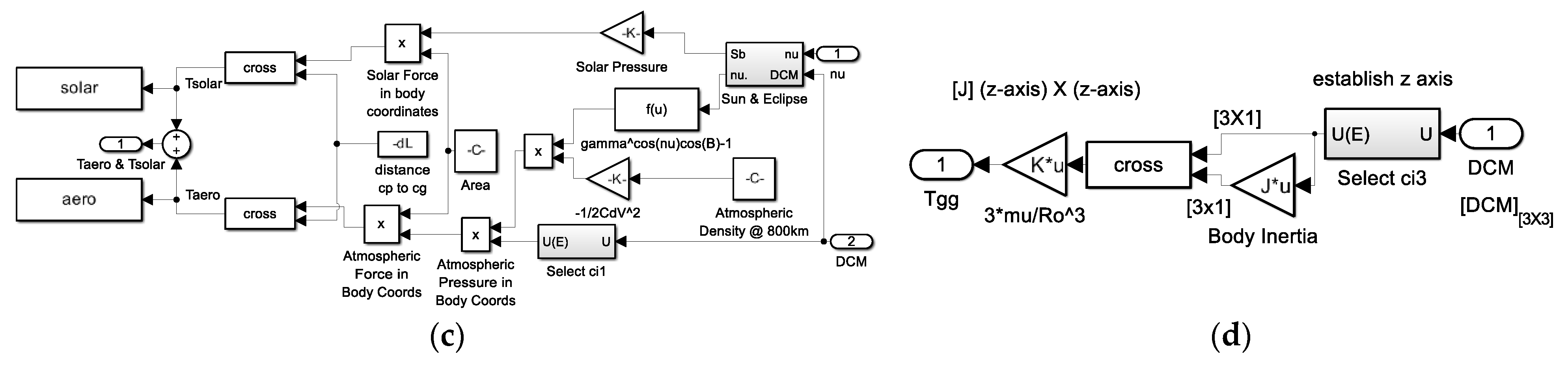
Autonomous robotic grappling (Figure 1) is the core requirement for on-orbit robotic servicing and assembly missions [1]. National Aeronautics and Space Administration (NASA) recently prototyped grappling arms for its Space Exploration Vehicle (SEV) [2].
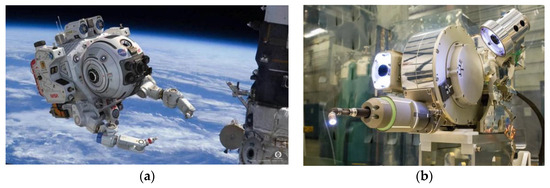
Figure 1.
(a) NASA PickNik Robotics in-orbit robot addresses a common gap in deploying robotic arms into environments where full autonomy is still too difficult permitting a human operator to supervise and quickly intervene when the space robot gets stuck [3]. (b) Robotic Refueling Mission 3 (RRM3) technologies are developed to store and transfer super-cold cryogenic fluids [4]. Image credit: NASA [5]. See ‘aside’ note in Appendix A.
1.1. Review of the Literature
The long-term sustainability of space includes other robotic tasks like active debris removal [6], necessitating arms for grappling and various grasping and anchoring mechanisms [2]. (Figure 1) According to the Technical Committee for Space Robotics of the IEEE Robotics and Automation Society, priority areas for the technical committee include electromechanical design and control, and command and control (including teleoperated modes) [7]. The study in reference [8] emphasizes center of mass changes due to deployment of payloads or instruments, solar panels, gravity booms, magnetometers, antennas, cameras, solar sails, etc., and used recursive least squares to estimate the mass center’s position. The study in [9] misaligns a thruster from the anticipated center of mass and uses the governing dynamic equations of motion to estimation the mass center location using multiple Kalman filters.
The determination of moments of inertia (but not inertia products) about two axes was proposed in 1948 for airplane components prior to flight, where the component would be suspended in a lab and subjected to standard pendulum experiments [10]. Similarly, the moments for the entire airplane were similarly treated in the study of [11]. Progress over the subsequent forty-six years added capabilities to use both angular acceleration methods and oscillation methods where the assumption is invoked that the suspension axis is assumed to be the axis of rotation [12]. Inertia cross-products were still not available. Twenty-nine years later, light detection and ranging was utilized to estimate inertia parameters within twenty percent, while location of the mass center was not performed [13,14]. Just this year, principal moments (not inertia cross products) of space tethers were estimated using unscented Kalman filters [15].
Mass center estimation was recently proposed using a force platform with inertial sensors for balance evaluation in quiet standing, and the results were compared to traditional methods using an optical motion capture system for truth values [16]. Three general classifications of methods were listed as follows, while this manuscript presents a novel alternative:
- Integrate the horizontal acceleration of the center of mass [17];
- Filter the center of pressure to estimate the center of mass [18];
- Estimate the center of mass directly from the equations of motion of an inverted pendulum model.
Ref. [19] categorized the methods slightly differently as either sensors’ networks or a single sensor while proposing using magneto-inertial measurement units. Calculation of the mass center was proposed [20,21,22] by electrostatic suspension of a proof mass in the satellite in an electrode cage, which is rigidly attached to the spacecraft. Accelerations of the proof mass were determined, and, then, relative accelerations between the spacecraft and proof mass were used to estimate the mass center. The procedure was used periodically to provide mass center location estimates. Follow-on experiments were presented in [23]. Arguably, this proof mass electrode cage may be considered state-of-the-art for spacecraft so equipped. The calculations involve estimations of angular velocities and quaternion fitting using regression (ASIDE: the methods proposed in this paper instead involve the estimation of all inertia components (moments and products) and use those estimates to deterministically calculate mass center location).
CFD methods were used in the study of [24] to investigate the aerodynamic performance of the free-fall wing, and the results indicate that wing fluttering and tumbling motions’ tumbling frequencies are driven by changing locations of the moments of inertia around the tumbling axis. Furthermore, the changing position of the center of mass complicates the free-fall motion. The study in reference [25] used least squares, maximum likelihood, and Kalman filter estimators to estimate mass, center of mass, and moments of inertia of a multi-lift slung aircraft load. The study in reference [26] used image processing to locate centers of mass using Python-based programming (Community Edition).
Regression-based learning may function as a projection operator to enable data-driven learning of the operators in the Mori–Zwanzig formalism, where the authors of [27] proposed a principled method to extract the Markov and memory operators for any regression models. The research found that more expressive nonlinear regression models fill in the gap between the highly idealized and computationally efficient Mori’s projection operator and the most optimal yet computationally infeasible Zwanzig’s projection operator.
For certain applications, e.g., the on-orbit debris inspection of orbital natural objects, defunct satellites, and debris, etc., estimating the mass center requires mapping from a moving observer. Ref. [28] applies an observer to estimate internal angular orientation, angular velocity, and angular acceleration. Next, pose-graph mapping with visual odometry produces trajectories relative to a target-fixed frame.
Distinguished from these disparate approaches to autonomously estimate the mass center (while maintaining the usage of observers), this present study seeks to determine time-varying inertia identification and the proposed novel online calculation of time-varying locations of the combined system’s center of mass using two norm optimal nonlinear, projection regression-based learning augmented with enhanced, nonlinear Luenberger observers in direct comparison to benchmark methods.
Box 1 provides pithy expressions of the manuscript’s problem statements, research objectives, and key contributions to the technical field(s). One additional courtesy offered the readership is periodic tables of proximal variables and nomenclature intended to eliminate the necessity to flip back and forth between pages (e.g. Table 1, Table 2, Table 3, Table 4, Table 5 and Table 6)
Box 1. Problem statements, research objectives, and key contributions
Problem statements: At all times, find a system’s mass distribution and the location of the center of mass. How may the location be calculated given only timed, angular position data? To what degree of accuracy can metrics be discerned? Requiring how much computational burden? Requiring how much effort?
Research objectives: (1) Using only attitude angle data, discern mass inertia imbalance, (2) express that imbalance as an offset center of gravity, and then discern the location of the center of mass.
Key contributions: Center of gravity location estimation convergence is improved over the state-of-the-art comparative benchmark [21,22,23] from millimeter convergence over hundreds of days to hundreds of millimeters in minutes achieved in this study.
1.2. State-of-the-Art Benchmarks
The following list highlights the current state-of-the-art inertia moment and product determination as well as locating the mass center:
- In 2022, Ref. [1] provided an overview survey of the algorithms and test and validation strategies for grappling the robotic free-flying spacecraft, de-emphasizing spacecraft docking and berthing. Core technologies identified includes orientation control (including distributed control systems) and the ability to adapt to unexpected loads. Those core technologies motivate the developments presented in this present study.
- Nonlinear dynamics are highlighted as key, and, therefore, nonlinear approaches are adopted.
- Despite insistence on nonlinear dynamics, linear time-invariant PID control laws are emphasized to be “straightforward to design and relatively easy to tune and provide performance sufficient to meet most operating requirements”.
- Since the dynamics are Hamiltonian, nonlinear adaptive control is also highlighted and adopted in this present study.
- Trajectory planning is highlighted as well, and autonomous trajectory generation is adopted to permit nonlinear control proposals.
- Air-bearing tables are highlighted to aid validation using laboratory experiments, and one such free-floating, highly flexible robotic gripper arm is described.
1.3. Novelties Presented
The following short list of novelties are combined sequentially to produce novel, autonomous, real-time space robotics:
- Time-varying estimates of mass locations are found with classical adaptive methods compared to optimal learning leveraging nonlinear, projection regression-based methods. Estimates are supported in part by the novel use of nonlinear enhanced Luenberger observers.
- Time-varying estimates of mass locations are used to find time-varying estimates of the location of the system center of mass. Estimates are supported in-part by the novel use of nonlinear enhanced Luenberger observers applying the fundamental relationships between products of inertia and mass center location.
- The requirement to diagonalize the matrix of mass moments of inertia is eliminated.
- The requirement to linearize the governing differential equations is eliminated.
- The requirement to simplify governing equations (e.g., small angle assumption, etc.) is eliminated.
- Analysis precedes modeling and simulation to verify the design, and then, spaceflight experiments are proposed for the sequel to validate the simulation results.
1.4. Conveniences of Presentation
Periodic tables of proximal variables and nomenclature definitions are provided to aid reading without necessitating flipping back and forth between pages seeking definitions of terms. Observers are presented topologically rather than using state space equations to aid remembrance and understanding. Lastly, simulations used to produce the data presented in this manuscript are used to produce the graphic topologies, and, furthermore, MATLAB®/SIMULINK® (R2023b) subsystems are included in the article Appendix, aiding repeatability by the readership.
2. Materials and Methods
Physics-based dynamics are foremost detailed in Section 2.1. Next, feedforward control using physics-based dynamic embodiment is presented in Section 2.2. followed by feedback instantiations: both the nonlinear adaption and projection regression-based learning of fully populated inertia matrix components. Nonlinear, enhanced Luenberger observers were introduced to support both feedback instantiations, and the observers were juxtaposed quantitatively to a comparative benchmark. Finally, location of the mass center was estimated using the estimated inertia components with the Final Value Theorem, which is briefly reviewed in the analysis of Section 2. As displayed in Figure 2, the canonical process is adopted of foremost analysis, followed by verification using modeling and simulation with experimental validation. Figure 3 displays the modeling and simulation topology.

Figure 2.
Process stages adopted in this study: analysis and hypothesis followed by the verification of analysis with modeling and simulation validated experimentally.
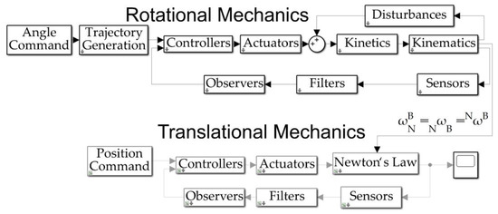
Figure 3.
Space robot system topology represented by the MATLAB®/SIMULINK® simulation used to produce the quantitative results presented in this manuscript. The internal content of simulation subsystems is depicted in Appendix B. Notice that the translational subsystems of the six-degree-of-freedom motion simulation are deactivated, reducing the superfluous computational burden.
Foreshadowing the summarized methods, Here includes a pithy implementation procedure and lists the relevant sections and details that may be found.
Implementation procedure:
| 1 | Use the physics-based governing dynamics to embody the control (Section 2.1). |
| a | Do not diagonalize the inertia matrix. |
| b | Do not linearize the governing equations of motion. |
| c | Do not use small-angle assumption to simplify the system equations. |
| d | Establish classical feedback control as a comparative benchmark. |
| 2 | Use nonlinear, enhanced Luenberger observers (Section 2.4, Section 2.5 and Section 2.6) to estimate all motion states and control. |
| 3 | Use projection-based nonlinear regression learning to learn the fully populated mass moments of inertia (masses and mass locations), including principal moments and off-diagonal products of inertia (Section 2.3). |
| 4 | Use off-diagonal products of inertia to estimate the location of the center of mass (Section 2.10). |
2.1. Physics-Based Dynamics
The well-known Euler’s moment equations (Equation (1)) govern rotations of objects of mass. The system of equations is nonlinear and coupled (especially for a fully populated inertia matrix with both moments and products of inertia), particularly noting the presence of the cross-product operation, which puts terms from the second and third equation into the first equation in the system. The equations were ubiquitously linearized and simplified by changing the basis of measurement to diagonalize the inertia matrix.
One motivation for linearization is to aid expression of the system of equations in a standard regression form (a matrix of ‘knowns’ multiplied by a vector of presumed ‘unknowns’). Particularly stemming from a common practice to put the motion states into the vector of unknowns, often referred to as the “state vector”, attempts to express Equation (1) into regression form can be seen in Equation (2).

Table 1.
Table of proximal variables and nomenclature (1) 1.
The inertia matrix is most often diagonalized using the eigenvalue coordinate transformation, or spectral decomposition. The transformation begins with relationships expressed in coordinates of the body fixed axes (where the inertia matrix is fully populated with moments and products). Transformation to a new basis vector set (i.e., the eigenvectors) leads to a diagonalized inertia matrix with only moments and no products, and the diagonalized matrix simplifies subsequent mathematics that are performed with the inertia matrix [29].
A common engineering practice is to simply assume the eigenvector basis is equivalent to the body frame basis vectors, where the engineer is comfortable accepting the accompanying error of such an assumption.
The inertia matrix will not be diagonalized in this present study, instead favoring increased accuracy. The inability of expressing Equation (2) in standard regression form must be re-addressed.
Noting the difficulties of Equation (2), omitting the common practice establishing the vector of unknowns, the mass moments and products may instead be used (Equation (3)). A more elaborate derivation from Equation (1) to Equation (3) is offered in Appendix A.
Equation (3) establishes the physics-based embodiment of the control with specific instantiations in both feedforward and feedback.
2.2. Feedforward Control Using Physics-Based Dynamic Embodiment
The feedforward instantiation of Equation (3) is presented in Equation (4), where the matrix of “knowns” necessitates having known angular velocities and angular accelerations. This necessity motivates the use of sinusoidal commanded trajectories, which will be shown to also aid estimation identifiability in Section 2.11.
This embodiment may also be used in feedback, where actual trajectories are substituted for desired trajectories, and that instantiation is described later in Section 2.10, Combined Control.
Table 2.
Table of proximal variables and nomenclature (2) 1.
2.3. Regression-Based Projection for Learning
Feedback may be used to project trajectory tracking errors (Equation (5)) on the nonlinear, coupled system equations expressed in regression in Equation (4). The estimated torque is not likely provided by motion sensors (e.g., star trackers, sun sensors, limb lookers, etc.), so observers are investigated to provide the information (in addition to full state trajectories described later in Section 2.10.
2.4. Luenberger Observers
Luenberger observers are sometimes referred to as state observers or simply observers and are well described in reference [30] for observable systems recently ubiquitously defined in so-called “state space” form or alternatively formulated in state-variable form. The discrete form of the estimator is often represented by the form presented in Equation (7) for discrete time index , states designated , the “hat” ^ indicating an estimate, output , where is the discretized state matrix, and is the discretized observer gain matrix, respectively.
Rather than adopting the ubiquitous form of Equation (7), observers are presented in the sections below in topological form to highlight the enhancements to the observers.
2.5. Enhanced Luenberger Observers
Notice in Figure 4 the three channels on the right-hand side of the figure. The ubiquitous derivative channel is past forward (to the left of the graphic) of the next integrator compared to the integral and proportional channels. Since the signal to the left of an integrator (the integrator output) is the integral of the input signal, the input signal (to the right) is the derivative of the output signal, thus inducing derivative action on the input. This commonplace enhancement induces derivative action into the estimator without numerically differentiating noisy input signals.
Secondly, notice that the top-center topology in Figure 4 contains a manual switch with the control as a potential input. This enhancement is often applied to reduce or eliminate phase lag in the estimator.
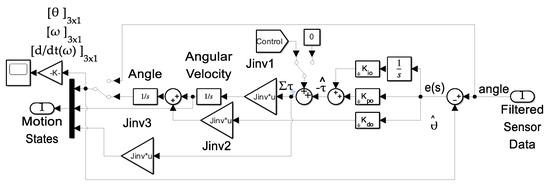
Figure 4.
Luenberger and enhanced Luenberger observers built in MATLAB®/SIMULINK®.
Lastly, notice that the center channel or line passing down the middle of the estimator from right to left consists of a double integrator of states lacking the cross-products of motion stemming from the transport theorem of mechanical motion relating the time derivative of a Euclidean vector as evaluated in a non-rotating coordinate system to its time derivative in a rotating reference frame [31]. Adoption of enhancements accounting for transport theorem are presented below, including nonlinear enhancements accounting for the nonlinear coupling nature of the transport theorem terms (the cross-products in Equation (1)).
2.6. Nonlinear Enhanced Luenberger Observers
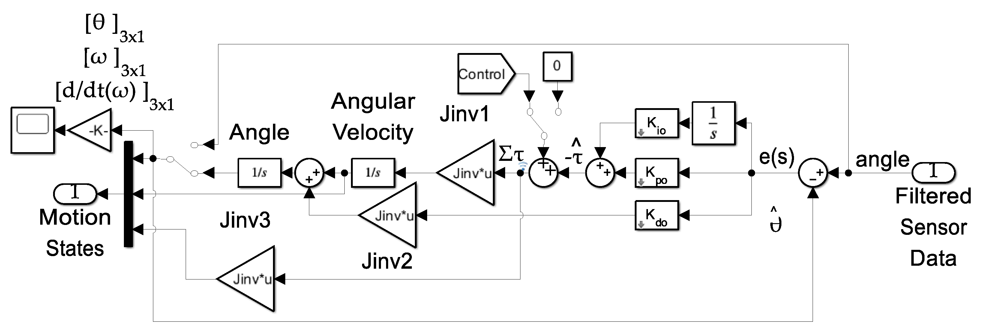
Notice Figure 5 contains predominantly the same content as Figure 4, the enhanced Luenberger observer. The new enhancements are depicted in the center of Figure 5 where the angular velocity signal is extracted, scaled by the mass moments of inertia, then used to create the cross-products which are added to the baseline double-integrator signal.
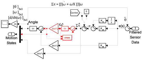
Figure 5.
Nonlinear enhanced Luenberger observer built in MATLAB®/SIMULINK®.
2.7. Classical Feedback Adaption
Following initial parameterization in the inertial reference frame, classical feedback adaption was presented in the study of [32] in the body reference frame, greatly simplifying the algorithms, enhancing its usefulness as a contemporary replacement of the formerly ubiquitous M.I.T. Rule [33]. The subsystem is displayed in Figure A5 of Appendix B, codifying Equation (8).
2.8. Two-Norm Optimal Nonlinear, Projection Regression-Based Learning
An alternative to the classical feedback adaption approach is to project trajectory tracking errors onto the governing system equations parameterized into nonlinear regression form (without truncation, approximations, linearization, diagonalization, or other implications). The regression form is illustrated in the feedforward ( portion of Equation (9)’s combined control, while the projection onto the system equations is displayed in the second term () using the two norm optimal pseudoinverse application of least squares. The subsystem is displayed in Figure A6 of Appendix B.
2.9. Combined Control
The feedforward control portion was identically the nonlinear, coupled governing equations of motion parameterized as a matrix multiplied by a vector where the matrix was built using desired (commanded) trajectories annotated by the subscribe “d”, while, in feedback form, actual trajectories were used in accordance with Equation (5). The need for actual trajectories justifies the investigation of contemporary enhancements to Luenberger observers in Section 2.4 and Section 2.5.
where is from Figure 4 and Figure 5.
2.10. Estimating Location of the Center of Mass
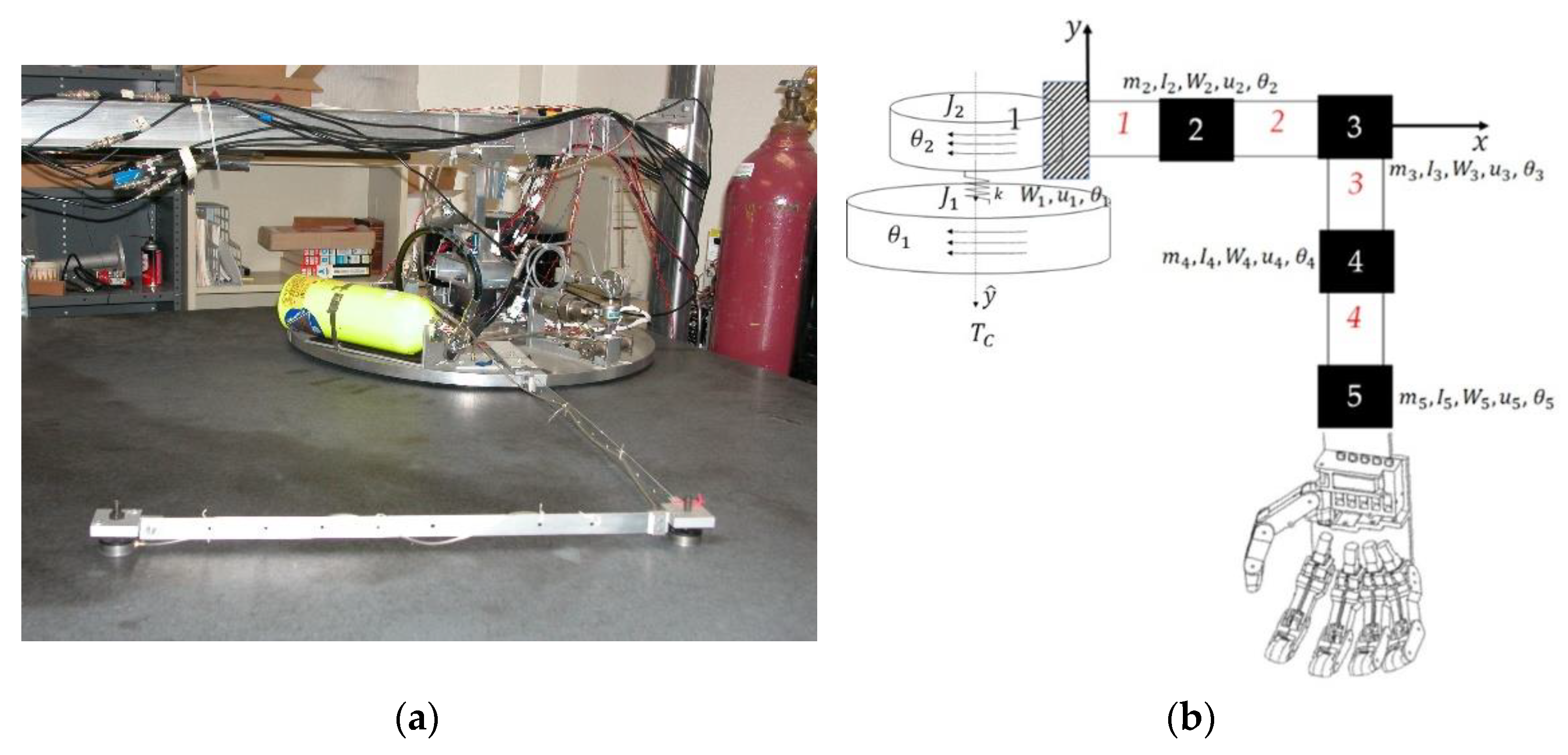
Since the matrix of mass moments of inertia was not diagonalized, the cross-products of inertia (off-diagonal matrix terms) may be used to locate the center of mass using the parallel axis theorem. Figure 6 provides an illustrative example. Consider the desire to have a mass center located along the depicted central axis. If the actual location is suspected to be at some other point, e.g., about the depicted axis, the parallel axis theorem may be used to parameterize the problem.
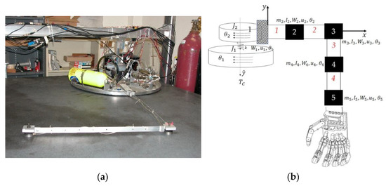
Figure 6.
Benchmark free-floating laboratory space gripper robot used in prequel studies [34]: (a) photo of laboratory hardware and (b) schematic used for prequel engineering analyses.
Table 3.
Table of proximal variables and nomenclature (3) 1.
Following a brief presentation of the parallel axis theorem with a small proof, the parameterization used to express three-dimensional locations ( coordinates) were revealed to be expressed strictly using the products of inertia. Thus, ubiquitous diagonalization of the inertia matrix by transforming basis vectors would eliminate the ability to use this formulation presented in Equation (12).
Theorem:
Parallel axis theorem: The moment of inertia about some point other than the center of mass is the sum of the moment of inertia about the center of mass and the moment of inertia relative to the fixed distance between axes ( and in Figure 6) in the rigid body represented by the product of the total mass and the square of the distance (See Equation (11)).
The following proof mirrors the study of [35], since the version most closely illuminates the use of the parallel axis theorem in this manuscript to reveal the three-dimensional location of the center of mass. The nomenclature of the proof in the study of [35] was mapped to the nomenclature of the formerly investigated space robot [34].
Proof:
Consider a rigid system of particles of mass , rotating about a fixed axis along axis . Place the origin of the coordinate system at the center of mass (cm) of our system of particles. The general point has coordinates (, ), the coordinate of is a, and the coordinate of is . Since the center of mass is at , by the definition of the center of mass (the unique point at any given time where the weighted relative position of the distributed mass sums to zero), Equation (12) results.
By definition, , where is measured from , not from the mass center. Thus, , leading to Equation (13). But, since and similarly for , the cross terms in Equation (13) go to zero once the sum over is achieved, leading to Equation (14). Since , where is now measured from the mass center, and is just , where is the distance from O to the mass center, Equation (15) results. □
Table 4.
Table of proximal variables and nomenclature (4) 1.
Equation (12) was extracted from the short proof of the parallel axis theorem, since it provides the time-varying location of the mass center giving known (or estimated) values of the products of inertia (which would not be available if the matrix had been previously diagonalized by transformation from the body axis basis to the eigenvector basis frame). Thus, the next necessary step of analysis is to elaborate the ability to estimate the inertia matrix, where moments and products together are used to embody the control, while the products of inertia alone are used to parameterize the location of the mass center.
2.11. Persistent Excitation of Estimation
Simple step commands do not provide sufficiently rich input signals to produce faithful estimates of system parameters and locations of the center of mass. More “rich” input signals were utilized to increase estimation confidence.
Definition 1:
Persistent excitation: Condition placed upon input commands to ensure that the signals provide sufficient information over time to accurately estimate system parameters (which eventually manifest as estimated locations of the system center of mass).
A finite impulse response model of order n involves the inversion of the matrix in Equation (16) where is defined in Equation (17) for control input signal . Estimation will have a unique solution (i.e., the process is “identifiable”) if and only if the matrix in Equation (16) is non-singular or invertible [36].
Table 5.
Table of proximal variables and nomenclature (5) 1.
Impacts of persistent excitation on parameter convergence are described in the study of [37]. Modeling accuracy requires the convergence of estimated parameters necessitating persistent excitation. Increased precision and faster convergence stems from relatively stronger excitation. The closed-loop stability of nonlinear, adaptive (or learning) systems was increased by bounding parameter estimation, which was also aided by persistent excitation. A step command has one instance of excitation and accordingly only leads to the reliable estimation of one parameter. Meanwhile, a sinusoidal command has two instances of excitation (as the curve oscillatory reverses direction twice) leading to the reliable estimation of two parameters. Random signals (i.e., Gaussian) are very rich excitation, since values at any pair of times are identically distributed, statistically independent (and hence uncorrelated), and, accordingly, aid the reliable estimation of any number of parameters. Accordingly, white noise was added to command signals in this investigation.
Table 6.
Persistent excitation of various input signals 1.
Propositions for achieving exponentially convergent estimation when lacking persistent excitation is presented in the studies of [38,39]. In this research, the approach taken is to add small amplitude white noise to all input command signals, which are based on sinusoids as constructed in Figure A1 (sinusoids) and Figure A3 (additional white noise) in Appendix B. The recommended input command is displayed in Box 2.
Box 2. Input signal recommendation
Recommended input command: To maximize persistent excitation, autonomous sinusoidal trajectories are recommended with white noise added.
2.12. Generic Robotics On-Orbit Trainer (GROOT) and Long-Duration Propulsive EELV Secondary Payload Adapter (LDPE ESPA)
A generic, customizable simulation is the basic orbital and robotic simulation (BOARS), developed and maintained by NASA simulations and the graphics branch [40], including two orbital vehicles as depicted in Figure 7 in arbitrary orbits. A robotic dynamic manipulator developed in collaboration with the United States Space Force (USSF) and used at the U.S. Air Force Test Pilot School was attached to one of the vehicles called the Generic Robotics On-Orbit Trainer (GROOT) [41]. The software simulations that were developed and used to produce the results in Section 3 of this manuscript utilized configurations scaled from those currently in use for the GROOT.
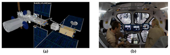
Figure 7.
(a) NASA basic orbital and robotic simulation (BOARS) [40] and (b) NASA exploration system simulations [41] for mission concept evaluation and operational insight to flight crew. Image credit: NASA, used in accordance with published image use policy [5].
2.13. Implementation Procedures
From Section 2, an implementation procedure immerges, summarized in Algorithm 1. The procedure was implemented using MATLAB®/SIMULINK® R2022b, where the subsystems are depicted in Appendix B to aid repeatability by the readership.
Using the implementation procedure in Algorithm 1, simulations were created (as depicted in Appendix B), and the results are next presented in Section 3.
| Algorithm 1 Pseudocode 1. |
| Input: Desired end state: final velocity and final acceleration |
| Output: Inertia matrix components and three-dimensional coordinates of the center of gravity |
| 1 begin |
| 2 Path planning using sinusoidal trajectories: |
| 3 DesiredVelocity = DesiredFinalVelocity * SineEquation |
| 4 DesiredAcceleration = DesiredFinalAcceleration * CosineEquation |
| 5 Assemble feedforward control |
| 6 Parameterize Euler’s moment equations into standard regression form |
| 7 Control_1 = DesiredStateMatrix * UnknownInertiaRegressionVector |
| 8 OptionalFeedback = DesiredStateMatrixInverse * EstimatedTorque |
| 9 EstimatedInertia = DesiredStateMatrixInverse * AppliedTorque |
| 10 MassCenterCoordinates = Function(InertiaCrossProducts) |
| 11 end |
| 1 Corresponding to Section 2. |
3. Results
This section presents the results of simulations of the proposed autonomous, online center of mass determination together with the nonlinear, coupled control and inertia identification and nonlinear, enhanced Luenberger observers.
3.1. Section Description
Section 3.2 describes the developed results incrementally beginning with the unperturbed system followed by the comparative benchmark. Introduced next is dynamic nonlinear feedforward augmented by (1) PID feedback and (2) inertia adaption. Next, dynamic, nonlinear feedforward with nonlinear, projection-based regression learning is applied. Estimation performance is compared next to evaluate Luenberger observer performance.
Section 3.3 performs the identification of mass moments and products. Identification is compared using nonlinear adaption versus nonlinear, projection-based learning. Section 3.4 extends the results of Section 3.3 to reveal the time-varying location of the center of mass again, comparing nonlinear adaption versus nonlinear, projection-based learning. While the baseline maneuver was a single thirty-degree yaw maneuver, compound maneuvers are evaluated next, before summary results are presented in Section 3.5.
3.2. Incremental Development and Presentation of Results
First, an unperturbed system is analyzed with classical feedback control. Next, a comparative benchmark for the study is analyzed, a highly perturbed system with classical feedback control. The perturbations include uniform variations to all values in the inertia matrix; random variations (white noise) added to the control to aid estimation; random noise added to sensor outputs; magnetic disturbance torques, aerodynamic disturbance torques, solar radiation pressure disturbance torques, and gravity gradient disturbance torques.
3.2.1. Unperturbed System
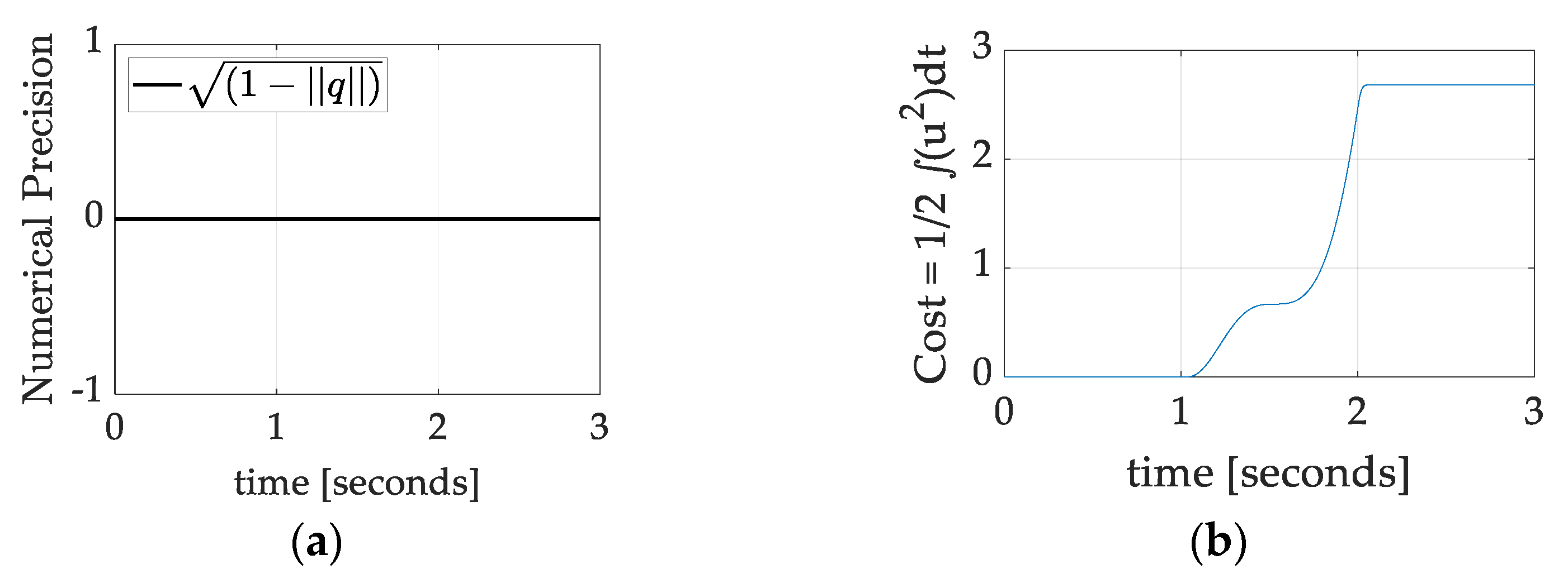
The unperturbed system is used to aid software troubleshooting and for investigating numeric precision. Numerical precision is studied using the quaternion normalization condition [42] displayed in Equation (18) as a figure of merit to iterate numerical integration solvers and evaluation step sizes. Solvers and step sizes were iterated until the error evaluating the quaternion normalization condition was always zero (or numeric zero), as displayed in Figure 8. Also displayed in Figure 8b is a display of the maneuver cost versus time, where the cost is calculated as one-half the time integral of the square of the control. Each case investigated is compared in part by the amount of control cost to perform the maneuver as one comparative figure of merit in addition to trajectory tracking error means and standard deviations.
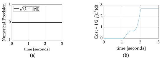
Figure 8.
(a) Quaternion normalization condition from Equation (18) used to validate numerical precision of simulation results. (b) Quadratic cost of maneuver.
The initial case investigated is classical PID control of an unperturbed system without feedforward or inertia adaption or learning, and the case is presented in Figure 9 and Figure 10 with quantitative data presented in Table 7.
Table 7.
PID-controlled unperturbed system.
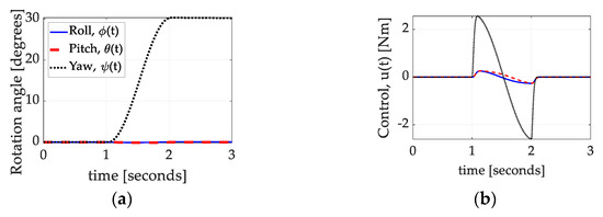
Figure 9.
(a) Rotation during unperturbed system maneuver: Thirty-degree yaw with time in seconds on the abscissa and rotation angle in degrees on the ordinant with roll as the solid blue line, pitch as the dashed red line, and yaw as the dotted black line. The three-dimensional maneuver data with time in seconds on the abscissa, roll as the solid blue line, pitch as the dashed red line, and yaw as the dotted black line presented together in Figure 9a are elaborated separately in Figure 10. (b) The control utilized during the maneuver. Quantitative data corresponding to the qualitative display in Figure 9 and Figure 10 are presented in Table 7.

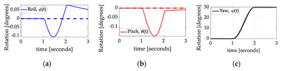
Figure 10.
Commanded rotation versus actual rotation during unperturbed thirty-degree yaw with time in seconds on the abscissa and rotation angle in degrees on the ordinant: (a) roll; (b) pitch; and (c) yaw. Commanded rotation versus actual rotation during highly perturbed thirty-degree yaw with time in seconds on the abscissa and rotation angle in degrees on the ordinant: (a) roll; (b) pitch; and (c) yaw. Quantitative data corresponding to the qualitative display in Figure 11 are presented in Table 7.
3.2.2. Comparative Benchmark
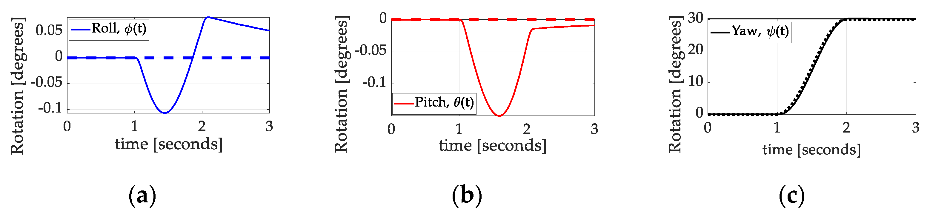
The comparative benchmark case of classical PID control without feedforward or learning controlling a highly perturbed system with sensor noise is presented in Figure 12 and Figure 13 with quantitative data presented in Table 8. Figure 12a simultaneously displays the roll, pitch, and yaw angles with respect to time. The commanded rotational maneuver is a thirty-degree yaw tracking a sinusoidal trajectory with no commanded roll or pitch, and the maneuver is performed with precision. The three axis controls are displayed in Figure 12b; notice the largest control corresponds to the yaw channel, while the relative smaller two channels of control counter the cross-coupled motion inherent with a fully populated inertia matrix. Figure 13 displays the same maneuver data as Figure 12a separated into three displays, one for each axis of motion: roll, pitch, and yaw. The three plots present qualitative information that matches the quantitative presentation of data in Table 8.
Table 8.
PID-controlled highly perturbed system: uniformly varied inertia, sensors with white noise, and thirty-degree yaw maneuver tracking errors.
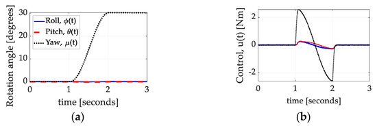
Figure 11.
PID control. (a) Rotation during unperturbed system maneuver: Thirty-degree yaw with time in seconds on the abscissa and rotation angle in degrees on the ordinant with roll as the solid blue line, pitch as the dashed red line, and yaw as the dotted black line. The three-dimensional maneuver data with time in seconds on the abscissa, roll as the solid blue line, pitch as the dashed red line, and yaw as the dotted black line presented together in Figure 11a are elaborated separately in Figure 12. (b) The control utilized during the maneuver. Quantitative data corresponding to the qualitative display in Figure 12 are presented in Table 8.
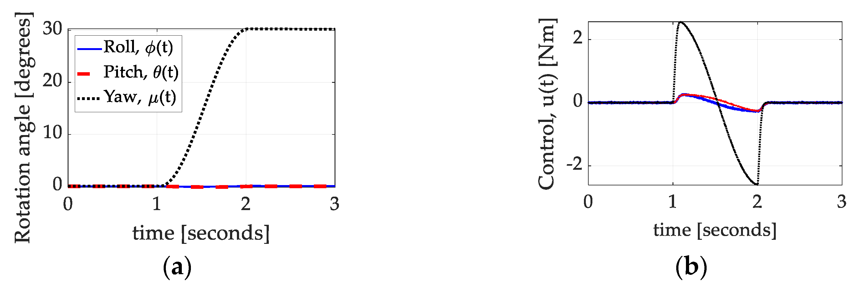
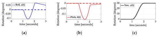
Figure 12.
PID-controlled highly perturbed system: uniformly varied inertia, sensors with white noise. Commanded rotation versus actual rotation during highly perturbed thirty-degree yaw with time in seconds on the abscissa and rotation angle in degrees on the ordinant: (a) roll; (b) pitch; and (c) yaw. Commanded rotation versus actual rotation during highly perturbed thirty-degree yaw with time in seconds on the abscissa and rotation angle in degrees on the ordinant: (a) roll; (b) pitch; and (c) yaw. Quantitative data corresponding to the qualitative display in Figure 12 are presented in Table 8.
3.2.3. Dynamic Nonlinear Feedforward with PID Feedback and Inertia Adaption
Having foremost established an idealized performance controlling an unperturbed system, next, the controlled system was perturbed with some performance degradation. Next, this section displays the results (in Figure 13, Figure 14, Figure 15, Figure 16 and Figure 17) of adding dynamic nonlinear feedforward and inertia adaption. Efforts were not made to optimize the adaption or the feedback gains, since tracking errors assist the estimation of the mass center location (the goal of this study). Estimation and tracking control is summarized in Box 3.
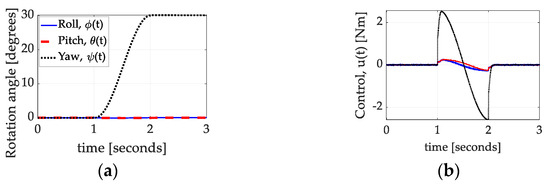
Figure 13.
Dynamic nonlinear feedforward with PID feedback and inertia adaption with roll as the solid blue line, pitch as the dashed red line, and yaw as the dotted black line: (a) Rotation during highly perturbed (uniformly varied inertia, sensors with white noise) thirty-degree yaw with time in seconds on the abscissa and rotation angle in degrees on the ordinant. (b) control versus time. Quantitative data corresponding to the qualitative display in Figure 14 are presented in Table 9.

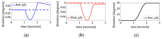
Figure 14.
Dynamic nonlinear feedforward with PID feedback and inertia adaption. Commanded rotation versus actual rotation during highly perturbed thirty-degree yaw with time in seconds on the abscissa and rotation angle in degrees on the ordinant: (a) roll; (b) pitch; and (c) yaw. Commanded rotation versus actual rotation during highly perturbed thirty-degree yaw with time in seconds on the abscissa and rotation angle in degrees on the ordinant: (a) roll; (b) pitch; and (c) yaw. Quantitative data corresponding to the qualitative display Figure 15 are presented in Table 9.

Table 9.
Dynamic nonlinear feedforward with PID feedback and inertia adaption. Highly perturbed (uniformly varied inertia, sensors with white noise) thirty-degree yaw maneuver tracking errors.
3.2.4. Dynamic Nonlinear Feedforward with PID Feedback and Nonlinear Projection-Based Regression Learning
Having, in the previous section, displayed the results of adding dynamic nonlinear feedforward and inertia adaption, this section replaces inertia adaption with nonlinear projection-based regression learning. As before, efforts were not made to optimize the adaption or the feedback gains since tracking errors assist the estimation of the mass center location (the goal of this study).
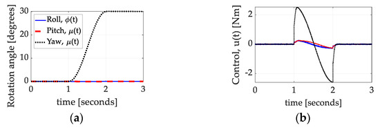
Figure 15.
Dynamic nonlinear feedforward with PID feedback and nonlinear projection-based regression learningwith roll as the solid blue line, pitch as the dashed red line, and yaw as the dotted black line: (a) Rotation during highly perturbed (uniformly varied inertia, sensors with white noise) thirty-degree yaw with time in seconds on the abscissa and rotation angle in degrees on the ordinant. (b) control versus time. Quantitative data corresponding to the qualitative display in Figure 15 are presented in Table 10.

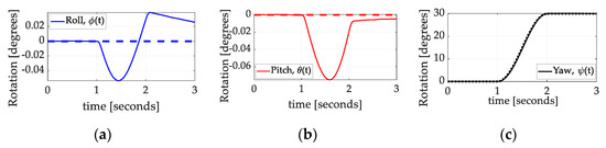
Figure 16.
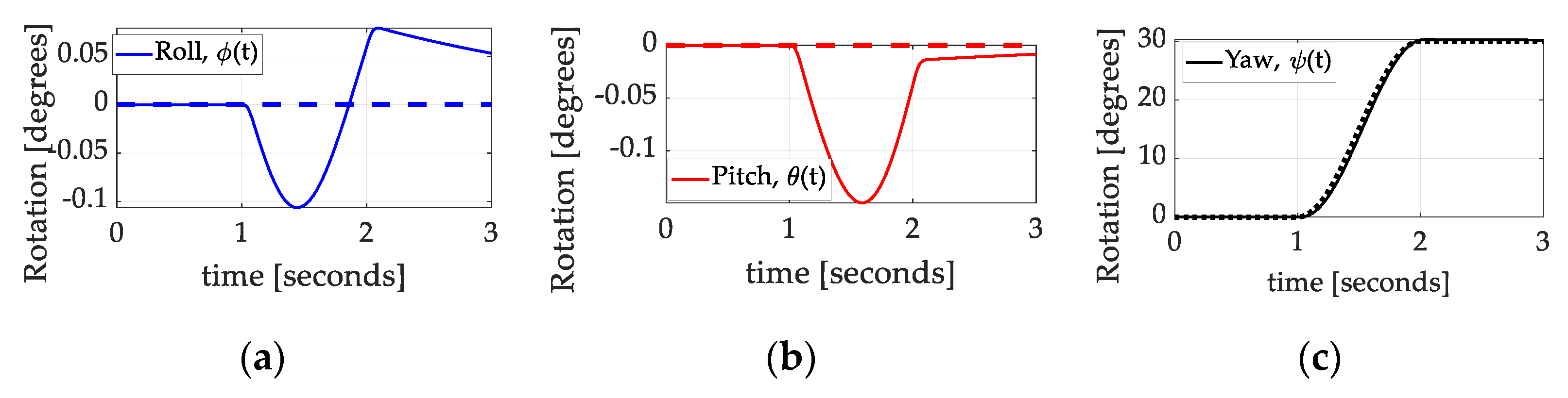
Dynamic nonlinear feedforward with PID feedback nonlinear projection-based regression learning. Commanded rotation versus actual rotation during highly perturbed thirty-degree yaw with time in seconds on the abscissa and rotation angle in degrees on the ordinant: (a) roll; (b) pitch; and (c) yaw. Commanded rotation versus actual rotation during highly perturbed thirty-degree yaw with time in seconds on the abscissa and rotation angle in degrees on the ordinant: (a) roll; (b) pitch; and (c) yaw. Quantitative data corresponding to the qualitative display in Figure 16 are presented in Table 10.
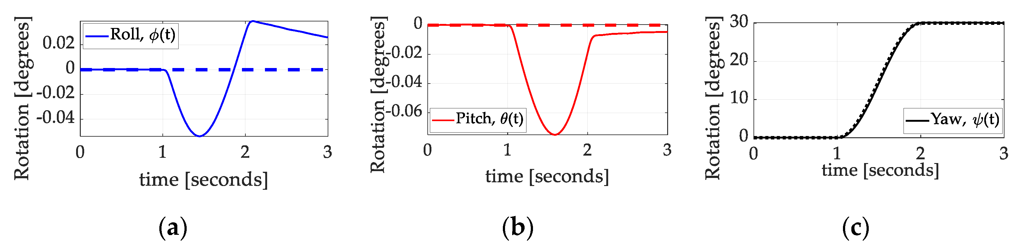
Table 10.
Dynamic nonlinear feedforward with PID feedback and nonlinear feedforward nonlinear projection-based regression learning. Highly perturbed (uniformly varied inertia, sensors with white noise) thirty-degree yaw maneuver tracking errors.
Box 3. Identical tracking: adaption vs. nonlinear projection-based regression learning
3.2.5. Estimator Performance Comparison
With the backdrop of introducing tracking control options, the remaining topic of study is the performance of state estimation by disparate Luenberger observers. Those estimated states are used by both the inertia adaption scheme and the nonlinear projection-based regression learning. The goal of the comparison is merely to choose the Luenberger instantiations. The observer comparison is presented qualitatively in Figure 18 and quantitatively in Table 11. The nonlinear, enhanced observer was slightly superior in the maneuver axis but relatively substantially inferior in the non-maneuver axes. Observer performance is presented in Table 11 and summarized in Box 4.
Table 11.
Observer estimation percent performance comparison. Highly perturbed (uniformly varied inertia, sensors with white noise) thirty-degree yaw maneuver tracking errors.
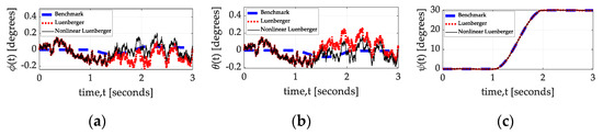
Figure 17.
Estimated actual rotation during highly perturbed thirty-degree yaw with time in seconds on the abscissa and estimated rotation angle in degrees on the ordinant: (a) roll; (b) pitch; and (c) yaw. The actual rotation angle (dashed blue line), the rotation angle estimated by the enhanced Luenberger observer (dotted red line), and the rotation angle estimated by enhanced, nonlinear Luenberger observers: (a) roll; (b) pitch; and (c) yaw. Quantitative data corresponding to the qualitative display in Figure 17 are presented in Table 11.

Box 4. Observer recommendation
Observer recommendation: Simultaneous use of both Luenberger styles is recommended to leverage their relative strengths in the maneuver axis and non-maneuver axis.
3.3. Identification of Mass Moments and Products
The estimations from the Luenberger observers are used to estimate inertia moments and products using two disparate methods: the nonlinear adaption and nonlinear projection-based regression learning described, respectively, in Section 3.3.1 and Section 3.3.2.
3.3.1. Identification of Mass Moments and Products by Nonlinear Adaption
Nonlinear adaption as proposed in the study of [43] and improved in the study of [32,44] were utilized to estimate the six inertia moments and products. The method was simulated in the study of [45] and experimentally validated in the study of [46].
A combined measure of error linearly combines angular acceleration and velocities using a constant gain. The gained, combined measure of error is multiplied by the system matrix with an adaption gain to establish the adaption rate, which is integrated to produce inertia component adaptions. The MATLAB®/SIMULINK® simulation subsystems are presented in Appendix B and the simulation results are displayed in Figure 18.
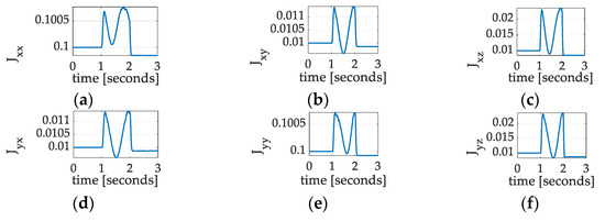
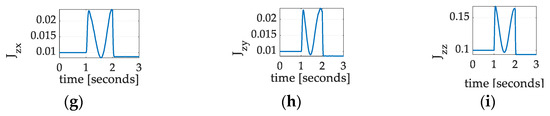
Figure 18.
Nonlinear adaption derived inertia moments and products: Time-varying mass moments and products for a single, thirty-degree yaw maneuver with coupled motion in roll and pitch, where the command has white noise added to aid persistent excitation (a) ; (b) ; (c) ; (d) ; (e) ; (f) ; (g) ; (h) ; and (i) . Notice that the initial flat-line behavior during the initial quiescent period is followed by rapid location learning during the maneuver excitement, lastly followed by a slow, oscillatory settling following the maneuver during regulation. The moments and products of inertia seem to converge towards a certain value during the maneuver excitation but not during either period of regulation, lacking persistent excitation.

3.3.2. Identification of Mass Moments and Products by Nonlinear Projection-Based Regression Learning
Nonlinear projection-based regression learning was proposed just last year in the study of [47] to learn the six inertia moments and products. Referring to Figure 19, the method that was utilized included an analysis and simulation, while validating experimentation is proposed in this present manuscript.

Figure 19.
Process stages adopted in this study: analyze and hypothesize followed by verification of analysis with modeling and simulation validated experimentally.
Angle trajectory tracking error alone (not in a combine error measure as performed with nonlinear adaption) is projected on the system matrix used to embody the nonlinear feedforward control parameterized in regression form without linearization, diagonalization, or otherwise simplification. Figure 20 reveals the mass moments and products estimated by the learning algorithm, while the corresponding MATLAB®/SIMULINK® simulation subsystems are presented in Appendix B.
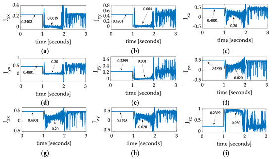
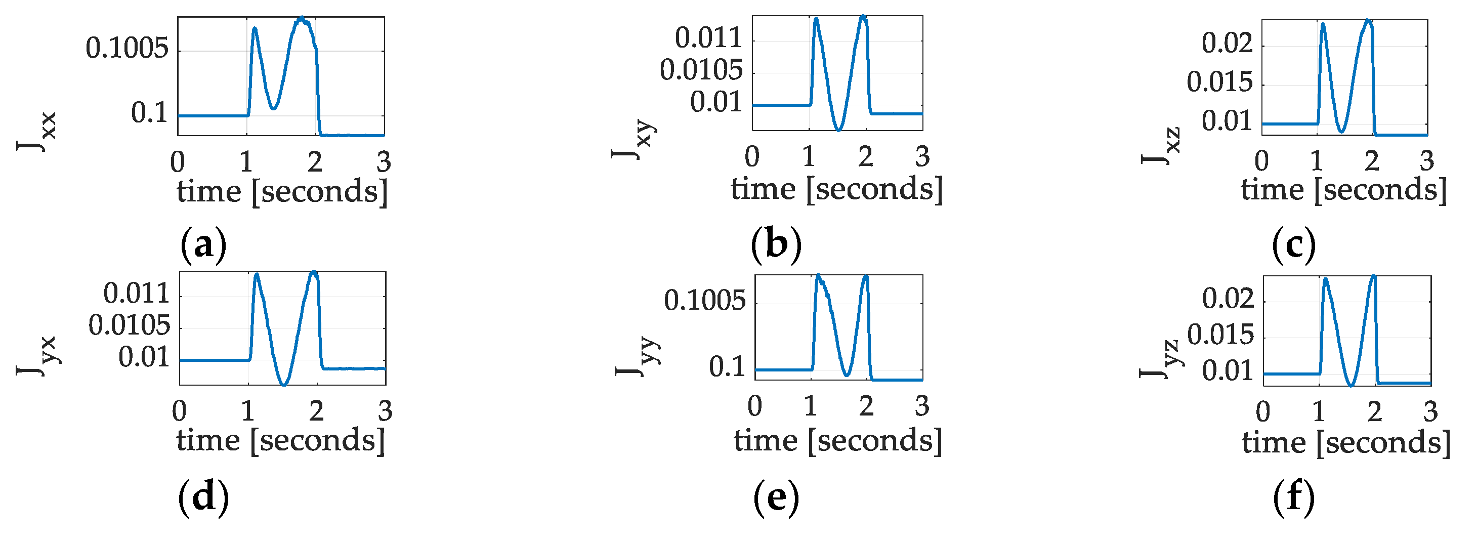
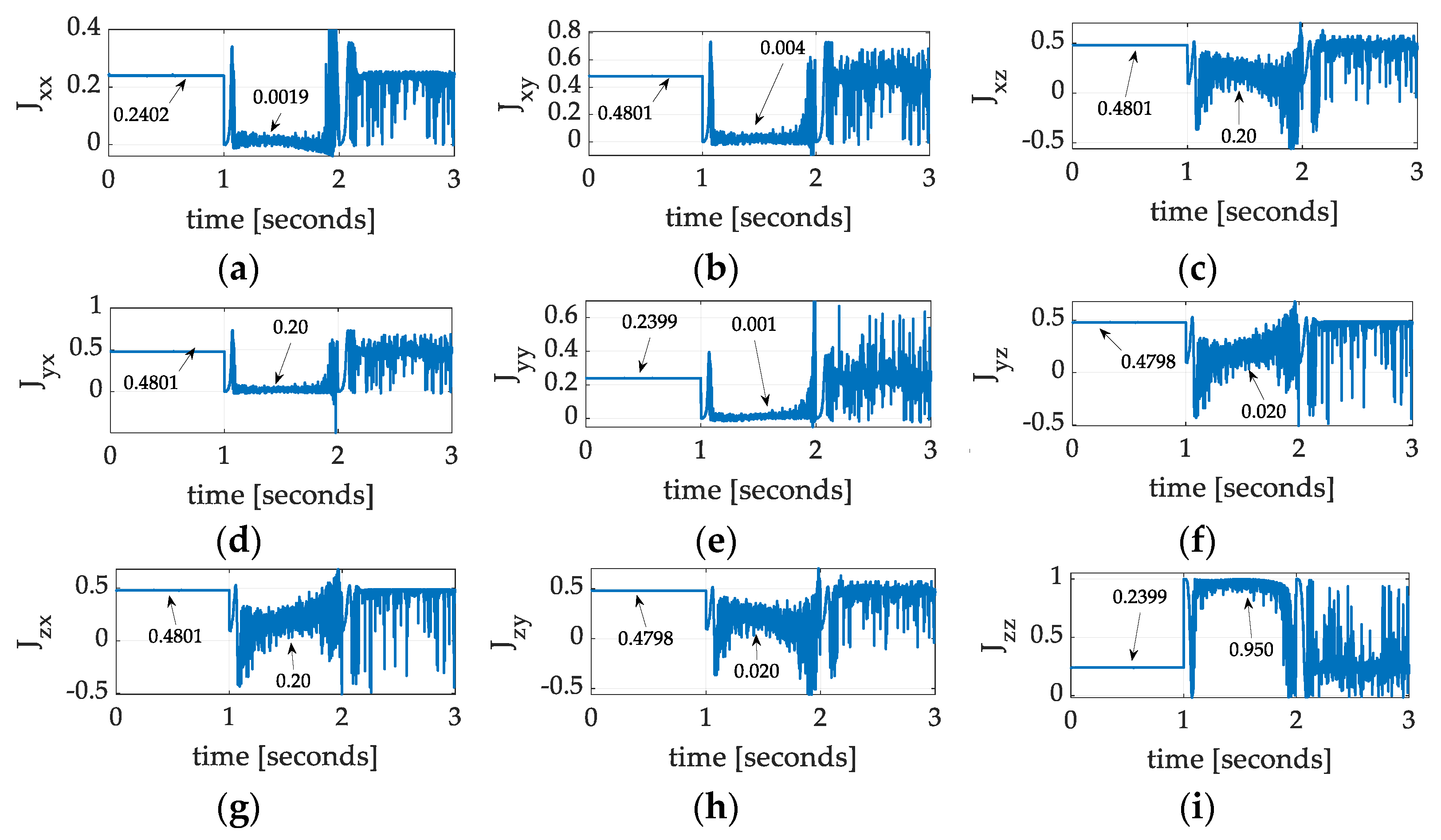
Figure 20.
Projection regression-based learning inertia moments and products: Time-varying mass moments and products for a single, thirty-degree yaw maneuver with coupled motion in roll and pitch, where the command has white noise added to aid persistent excitation (a) ; (b) ; (c) ; (d) ; (e) ; (f) ; (g) ; (h) ; and (i) . Notice that the initial flat-line behavior during the initial quiescent period is followed by rapid location learning during the maneuver excitement, lastly followed by a slow, oscillatory settling following the maneuver during regulation. The moments and products of inertia seem to converge towards a certain value during the maneuver excitation but not during either period of regulation, lacking persistent excitation.
3.4. Location of Mass Center
Time-varying estimates of mass moments and products may be used with Equation (12) to directly calculate the location of the mass center (as a reminder that the inertia matrix must not be diagonalized). The estimates of inertia moments and products are produced with two disparate methods: nonlinear adaption and nonlinear projection-based regression learning, respectively, in Section 3.4.1. and Section 3.4.2.
3.4.1. Identification of Mass Center Coordinates by Nonlinear Adaption
Notice in Figure 21 that adaption occurs twice: at the beginning and the end of trajectory tracking. The roll channel depicted in subfigure (a) seems to indicate a proper mass center location roughly at 0.15 in the direction. Meanwhile, the pitch channel adaption deviates from 0.1 in the direction, while the yaw channel location adaption displayed in subfigure (c) behaves similar to the roll channel, seemingly indicating a mass center location roughly 0.225 in the direction. Lastly, notice, during the post-maneuver quiescent period, that the location estimate does not return to the initial estimate (at the beginning of the pre-maneuver quiescent period). As a reminder, the control signal contains a sinusoidal trajectory command (which is persistently exciting of order 2) with white noise added (which is persistently exciting of order ). Efficacy towards mass center location is presented in Box 5.
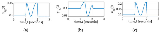
Figure 21.
Nonlinear adaption time-varying location of the center of mass: For a single, thirty-degree yaw maneuver with coupled motion in roll and pitch, where the command has white noise added to aid persistent excitation (a) coordinate; (b) coordinate; and (c) coordinate. Notice that the initial flat-line behavior during the initial quiescent period is followed by rapid location learning during the maneuver excitement, lastly followed by a slow, oscillatory settling following the maneuver during regulation. The location seems to approach the body axis origin in the and directions with slight movement away in the direction.
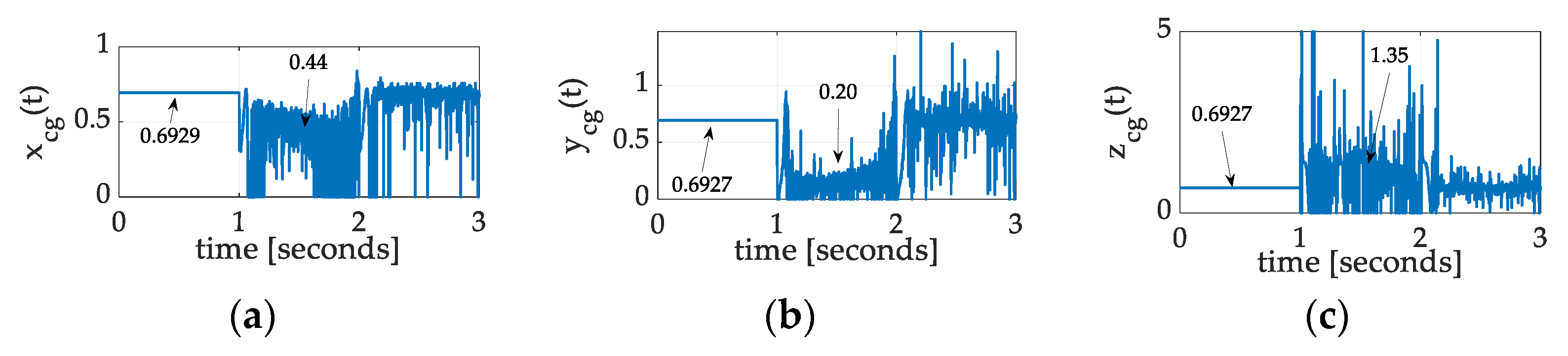
3.4.2. Identification of Mass Center Coordinates by Nonlinear Projection-Based Regression Learning
Notice in Figure 22 that adjustment occurs many more times than twice. Especially focusing on the period between the beginning and the end of trajectory tracking, the roll channel depicted in subfigure (a) seems to indicate a proper mass center location roughly at 0.44 in the direction. Meanwhile, the pitch channel adaption deviates from 0.20 in the direction, while the yaw channel location adaption displayed in subfigure (c) seemingly indicates a mass center location roughly 1.35 in the direction. Again, notice, during the post-maneuver quiescent period, that the location estimate does not return to the initial estimate (at the beginning of the pre-maneuver quiescent period). As a reminder, the control signal contains a sinusoidal trajectory command (which is persistently exciting of order 2) with white noise added (which is persistently exciting of order ).
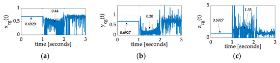
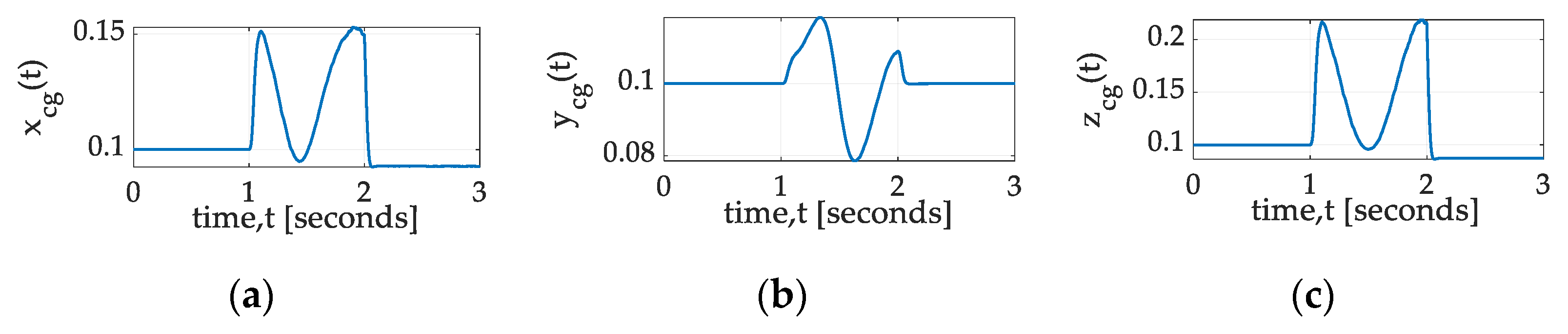
Figure 22.
Projection regression-based learning time-varying location of the center of mass: Three-dimensional coordinate estimates (a) , (b) , and (c) ; for a single, thirty-degree yaw maneuver with coupled motion in roll and pitch, where the command has white noise added to aid persistent excitation. Notice that the initial flat-line behavior during the initial quiescent period is followed by rapid location learning during the maneuver excitement. Furthermore, notice that the degree of convergence spans roughly 253, 493, and 657 mm in each axis, respectively, in mere seconds.
Box 5. Mass center recommendation
Locating the mass center: Compared to using nonlinear adaption, the use of nonlinear projection-based regression learning was more sensitive to identical cases of persistent excitation and accordingly produced better location of mass center.
3.4.3. Location of Center of Mass: Three-Dimensional Comparison
Both methods of inertia matrix components identification (adaption and learning) were implemented and compared in Figure 18, Figure 19 and Figure 20. Immediately evident upon first glance is the fact that the adaptive approach converges relatively slowly compared to projection regression two-norm optimal learning. While developing the learning approach in Section 2 of this manuscript, the notion of having optimal estimates at every time step seemed attractive but clearly has drawbacks illustrated in Figure 22 and Figure 23a compared to the nonlinear adaptive approach, whose results are displayed in Figure 21 and Figure 23b. The two norm optimal pseudoinverse calculations in the learning approach seem to be highly excited by the presence of so many perturbations (indicating potentially poor applicability to deployed space robotic systems).
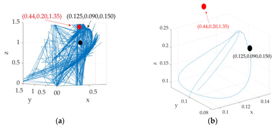
Figure 23.
Comparison, time-varying location of the center of mass: (a) three-dimensional plot of learned cg location using projection regression-based learning; (b) three-dimensional plot of learned cg location using nonlinear adaption for inertia calculations. Both (a,b) use identical deterministic relationships to locate the center of mass using the products of inertia.
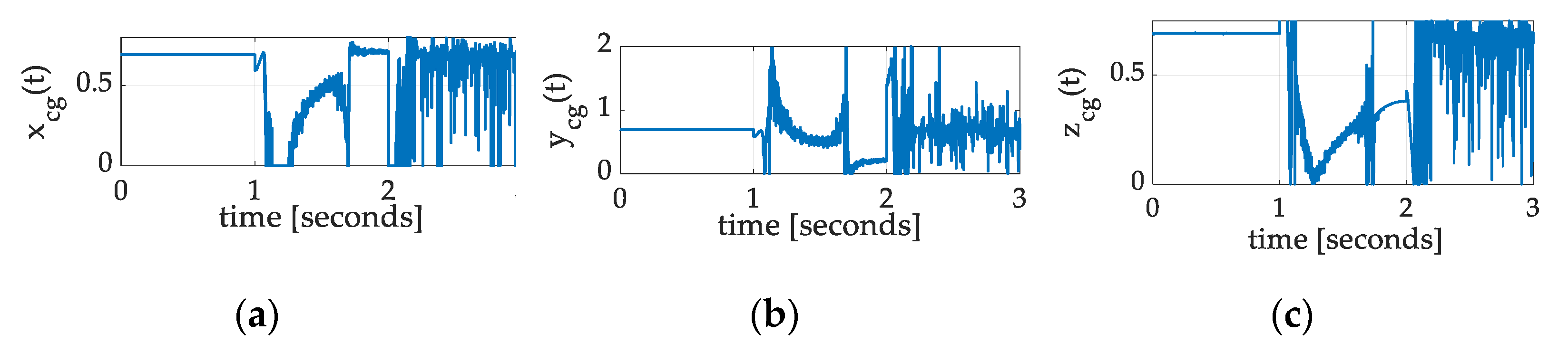
3.5. Compound Maneuvers
Compound maneuvers were investigated, and the results are summarized in Box 6 and displayed in Figure 24 and Figure 25 and Table 12.
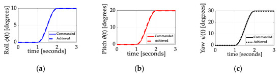
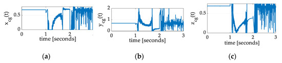
Figure 25.
Compound maneuver estimated mass center location. Projection regression-based learning with nonlinear Luenberger observers: (a) -coordinate; (b) -coordinate; and (c) -coordinate.
Table 12.
Compound maneuver trajectory tracking errors. Projection regression-based learning with nonlinear Luenberger observers.
Box 6. Compound maneuver recommendation
Single-axis versus compound-axis maneuvers: Compound maneuvers eliminated the learning convergence experienced with single-axis maneuvers. Single-axis maneuvers should be sequenced sequentially amongst all three axes.
3.6. Summary of Results
Results displayed in this manuscript are consolidated in this section and presented as percent performance difference relative to a comparative benchmark in Table 12, Table 13, Table 14, Table 15 and Table 16. Narrative results are subsequently discussed in Section 4 Discussion, aiming to highlight substantial results in plain verbiage (e.g., no use of “microradian”, etc.) in favor of percent performance difference. Superlative results are highlighted in bold font to amplify information transmission when readers scan this manuscript.
Table 13.
Attitude control trajectory tracking percent performance difference †.
Table 14.
Performance comparison of controlling highly perturbed system (uniformly varied inertia, sensors with white noise) 1 unless otherwise stated for a thirty-degree yaw maneuver.
Table 15.
Locating center of mass performance comparison ****, †.
4. Discussion
Nonlinear adaptive methods for locating the mass center proved effective but less so than nonlinear projection-based regression learning. Using identical excitation, nonlinear adaptive methods were able to establish an average seven percent difference in coordinates of the mass center, while an average over seventy percent difference was achievable using nonlinear projection-based regression learning. Listed in Table 16, several recommendations are advised to repeat these results.
Table 16.
Most significant recommendations.
Future Research Directions
While this prequel study introduces the first two steps of investigation (analysis and verification in simulations), validation with spaceflight experiments is planned for March 2025, after which a sequel will be published with the results of the spaceflight tests.
5. Conclusions
Arguably, reference [22] presents the best recently proposed comparative benchmark, since that method was experimentally validated on the GRACE-C satellite. The method effectively generated convergent estimates of mass center coordinates, where the convergence spanned just greater than 0.3 mm over several hundred days. Meanwhile, convergence using the proposed methods (in simulations) spans roughly 200–600 mm, respectively, in each axis, and convergence occurs in mere seconds, assuming a single-axis slew maneuver. Multi-axis, compound slew maneuvers were completely ineffective using the proposed approach to estimate coordinates of the center of mass. Succinctly, the proposed methods seem to indicate advantages of speed and the quantity of coordinate convergence when compared to the state-of-the-art comparative benchmark. Spaceflight experiments planned for March 2025 will evaluate the efficacy of this proposed approach empirically.
Funding
This research received no external funding. The APC was funded by the corresponding author.
Data Availability Statement
Data supporting reported results can be obtained by contacting the corresponding author.
Conflicts of Interest
The author declares no conflicts of interest.
Appendix A
The nonlinear feedforward is developed step-by-step in this Appendix.
Appendix B
This appendix displays all the simulation subsystems permitting repeatability by the readership using MATLAB®/SIMULINK®. Implementation steps are as follows:
- Create a scheme of command. A sinusoidal scheme is depicted in Figure A1 and may be constructed by dragging and dropping the blocks depicted from the library to the simulation. The switching logic produces smooth sinusoids for angular displacement, velocity, and acceleration. The switch institutes to regulation at the final commanded value, smoothly exiting the sinusoidal curves, respectively. The syntax for the sinusoidal commands is displayed in Figure A2.
- The attitude controllers are displayed in Figure A3, including both feedforward and feedback controllers. The project-based learning algorithm is also included. Additionally, notice that there is a manual switch away from the input sinusoidal trajectories and optionally towards a simple step command. Lastly, notice that artificially faked inertia values and random perturbations are included as switchable options as well.
The implementation steps elaborated so far in Appendix B yield an ability to produce endpoint commands, autonomous trajectory generation, and trajectory tracking abilities, where the outputs include the control torque (to be sent to the space robot). Additional outputs include time-varying inertia estimates and location of the center of mass. The control signal is routed to the actuator on the space robot.
- 4.
- The reaction wheel actuator is displayed in Figure A9, where the output torque from the actuator is routed to the governing equations of motion depicted in Figure A10 with expanded drilldown elaboration in Figure A11 and Figure A12. The governing equations of motion produce angular velocities relative to the inertial reference frame but need to be expressed in the coordinates of a body frame of interest.
- 5.
- Figure A12 displays the high-level kinematic topology. Drill downs for quaternions are displayed in Figure A13 where the quaternions are used to construct a nine-element direction cosine matrix transformation between inertial and body coordinates. The direction cosine matrix is used to extract Euler angles where a “321” rotation sequence is assumed, and that code is depicted in Figure A14.
- 6.
- While the true Euler angles cannot be known by the robot operators, sensors are simulated with additive noise and filters designed to counteract the noise in Figure A15.
- 7.
- The direction cosine matrix conveniently reveals the vector locations of the body axes and is used to calculate environmental disturbance torques.
The implementation steps elaborated so far in Appendix B now additionally include kinetics, kinematics, noisy sensors, and filters. Lastly, the simulation of environmental disturbances is elaborated.
- 8.
- The top-level topology of environmental disturbances is displayed in Figure A16 where each subsystem is individually displayed in Figure A17 for atmospheric, magnetic, solar radiation, and gravity gradient disturbances.
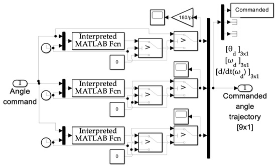
Figure A1.
Internal content of trajectory generation subsystem depicted in Figure 3. Notice the sinusoidal attitude trajectories are formulated from the single input of angle commanded outside the space robot (presumably either autonomously by the demands of the translational motion subsystem or alternatively externally supplied by a human operator aiding the space robot’s motion with remote-controls).
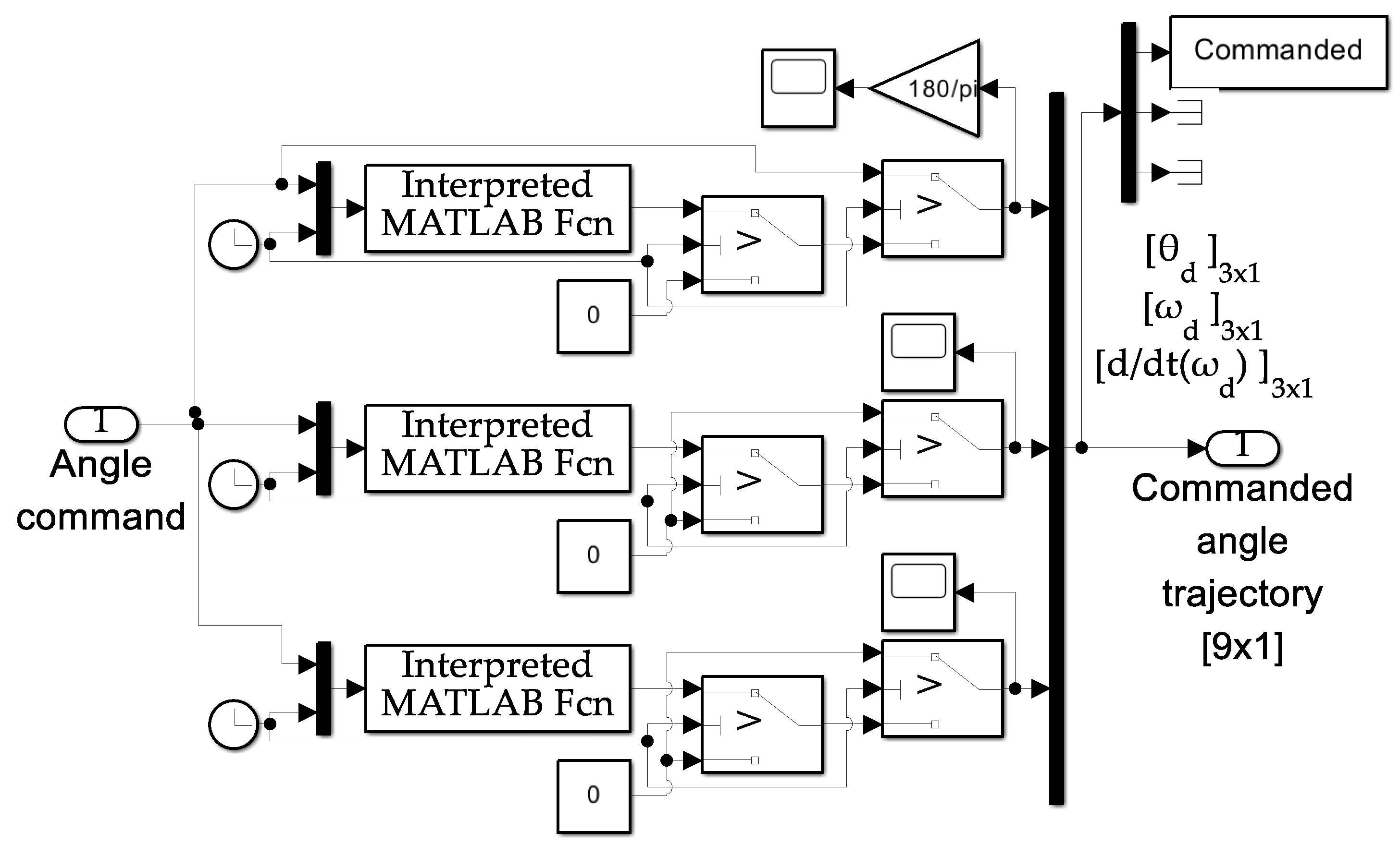
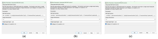
Figure A2.
Pseudocode (labeled “Block Parameters”) used in the three “Interpreted MATLAB Fcn” blocks in Figure A1 encoding the angle (a), angular rate (b), and angular acceleration (c) commands, respectively. Top-to-bottom subsystems in Figure A1 correspond to left-to-right block parameters in this figure. The pseudocode is provided to aid repeatability of the research results.
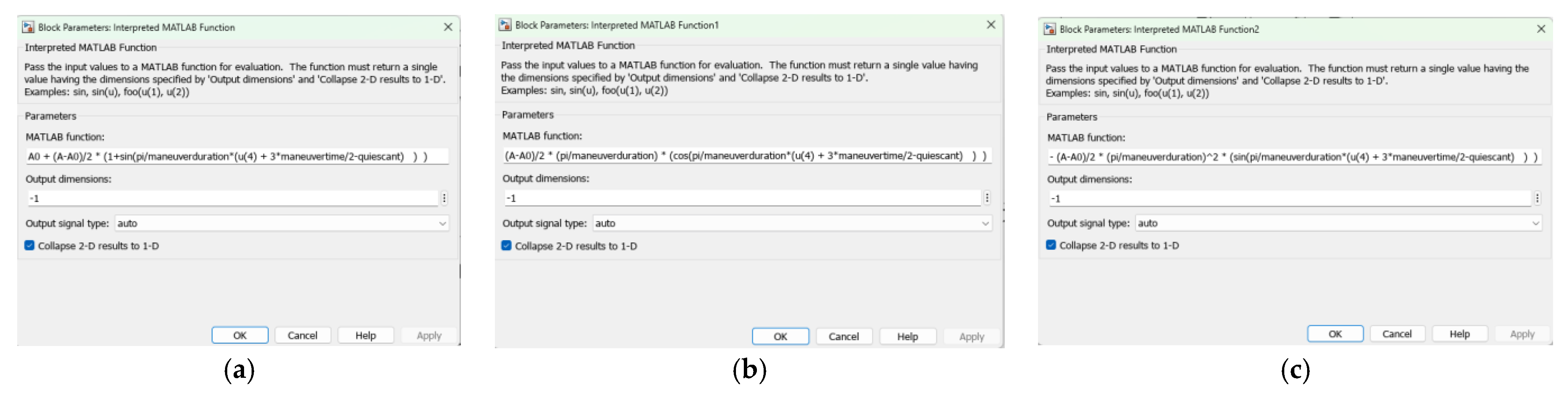
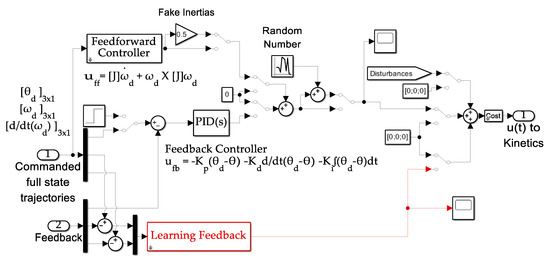
Figure A3.
Internal content of “Controllers” subsystem depicted in Figure 3. Notice the use of manual switches permitting simulation iteration where all facets are held constant except the facet being investigated. Furthermore, notice the “fake inertia” gain block at the center-top of the figure permits simulation users to artificially make the feedforward command (based on the assumed values of the mass moments of inertia) artificially smaller or larger that assumed. Doing so permits simulation debugging, e.g., if the user artificially makes the mass moments to be assumed much larger, the learning feedback should produce the adaption of mass moments towards the values manually altered in the gain block.
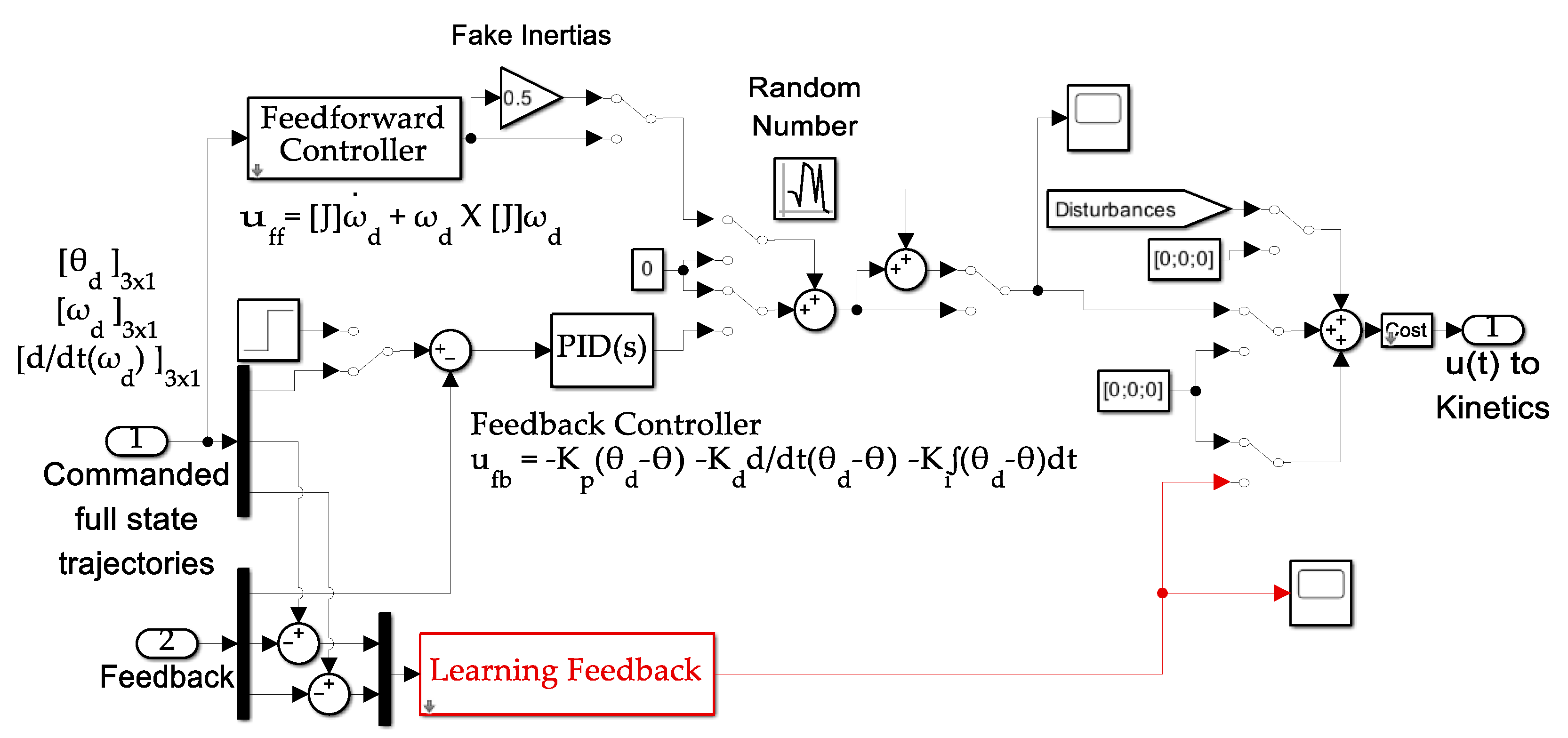
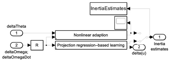
Figure A4.
Internal content of “Learning Feedback” subsystem.

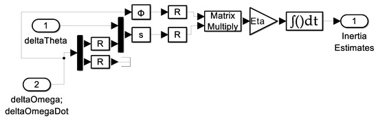
Figure A5.
Internal content of “Nonlinear adaption” option in the “Learning Feedback” subsystem.
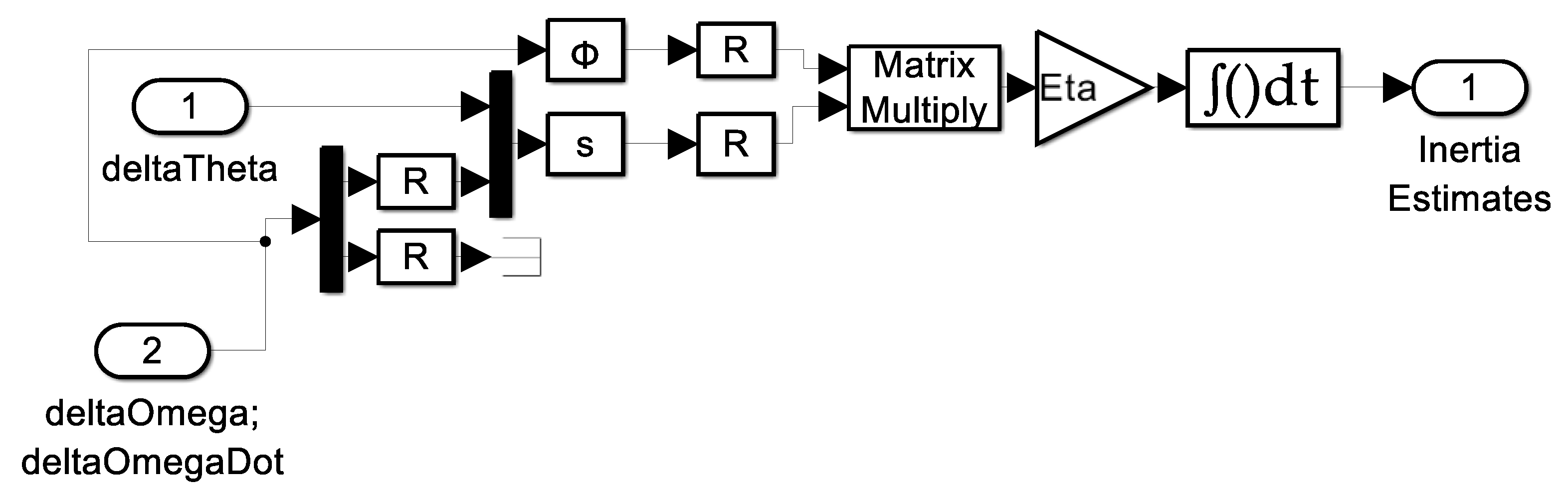
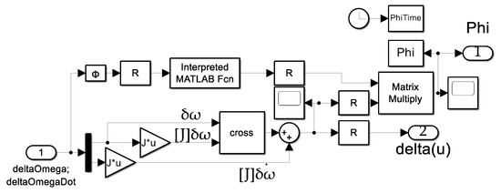
Figure A6.
Internal content of “Projection regression-based learning” option in the “Learning Feedback” subsystem.

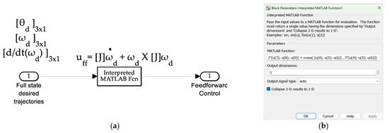
Figure A7.
(a) Internal content of “Feedforward Control” subsystem in Figure A3. (b) Internal pseudocode of the “Interpreted MATLAB FCN” block in subfigure (a).
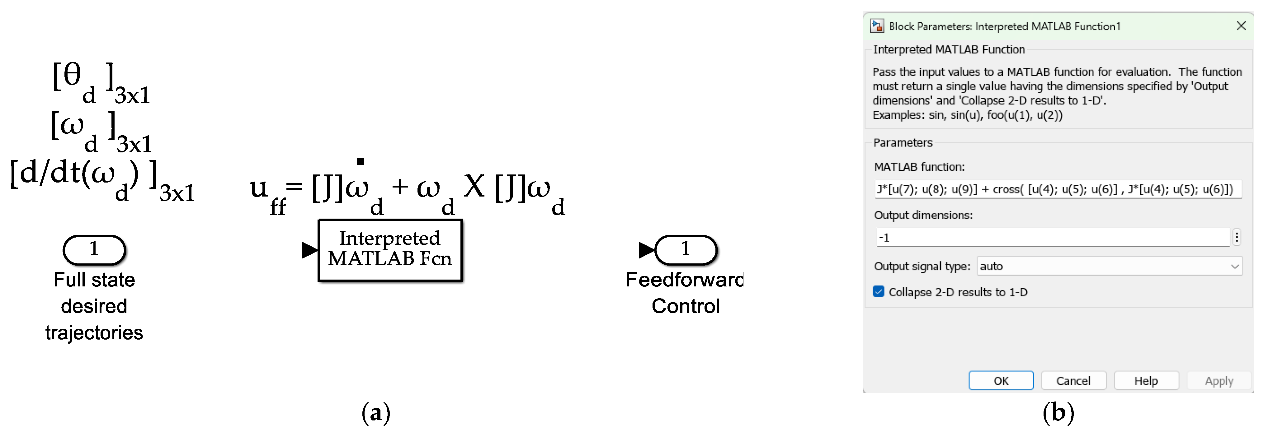

Figure A8.
Internal content of “Learning Feedback” subsystem depicted in Figure A3.
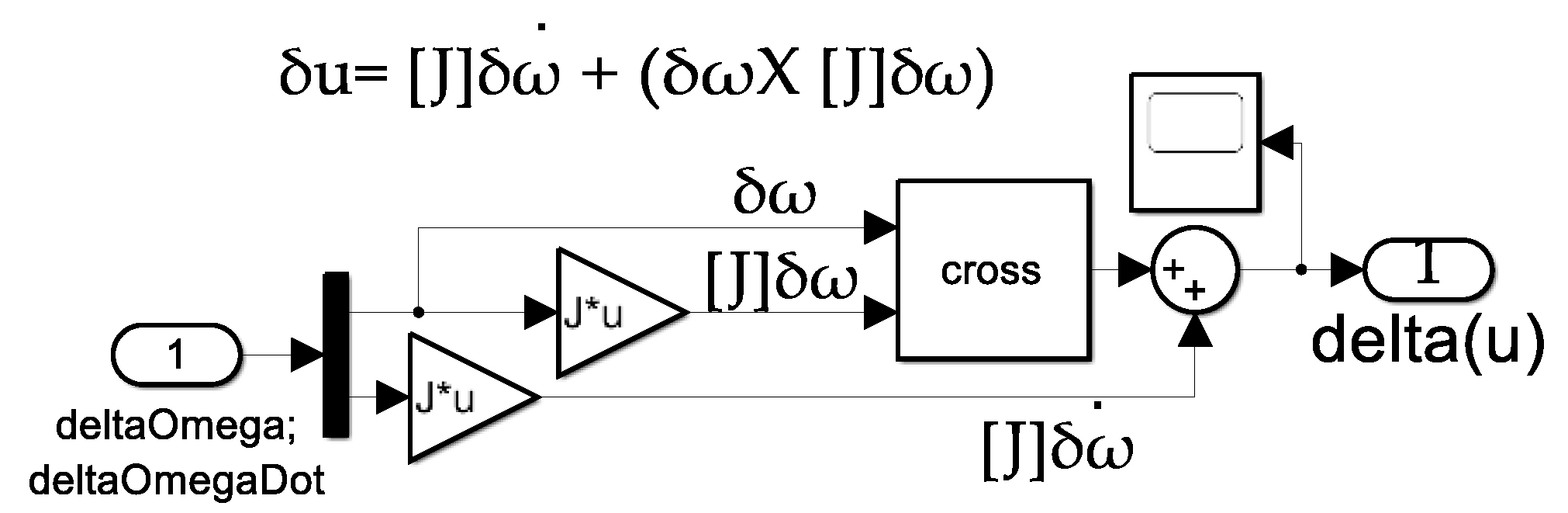

Figure A9.
Internal content of “Actuators” subsystem depicted in Figure 3.
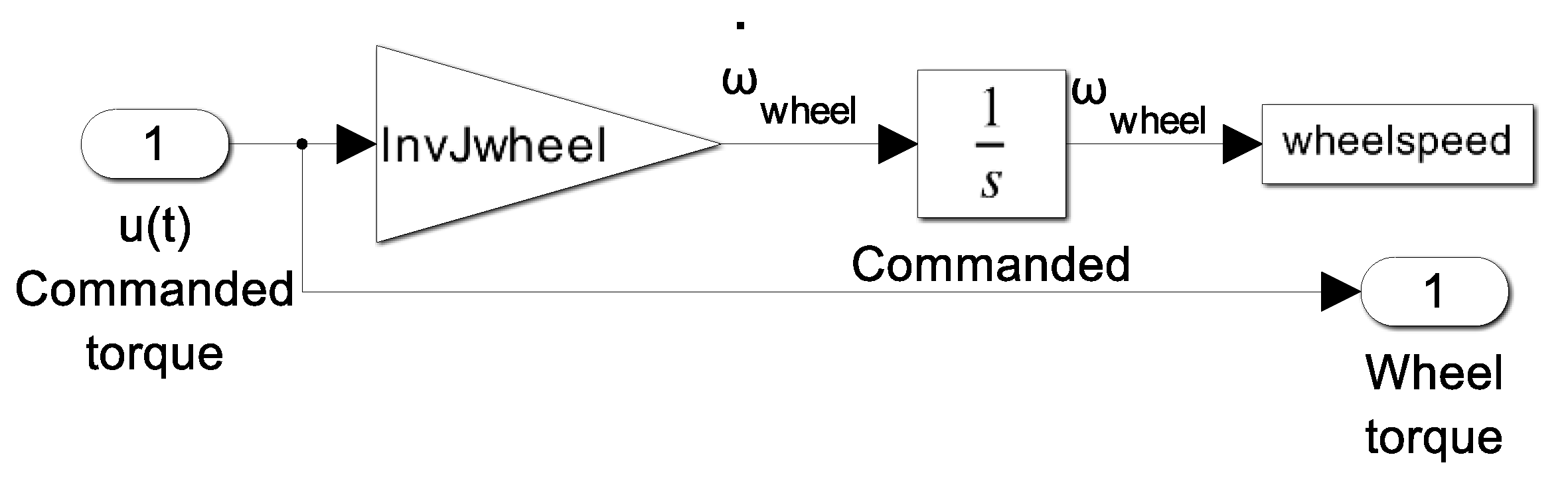

Figure A10.
Internal content of “Kinetics” subsystem depicted in Figure 3. The upper two subsystems are elaborated in Figure A11, while the final (lowest) kinetic system is the simple integrator depicted on the bottom of this figure.
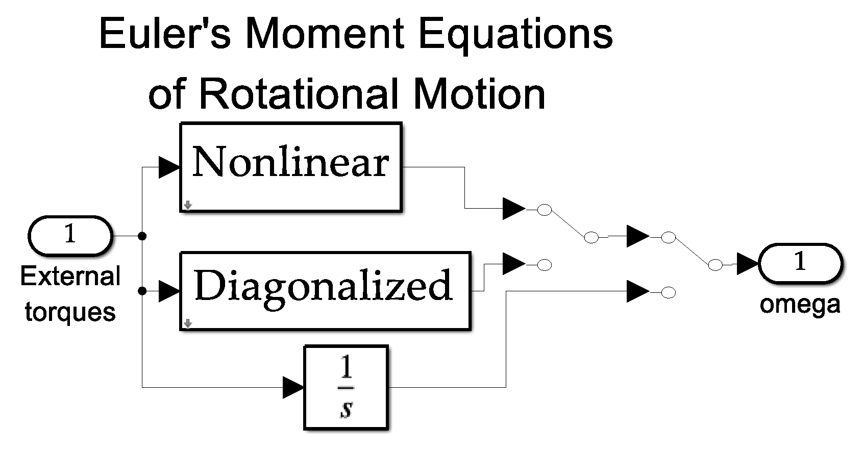
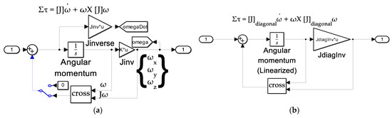
Figure A11.
(a) Internal content of “Nonlinear” kinetics subsystem depicted in Figure A10. (b) Internal content of “Diagonalized” kinetics subsystem depicted in Figure A10.
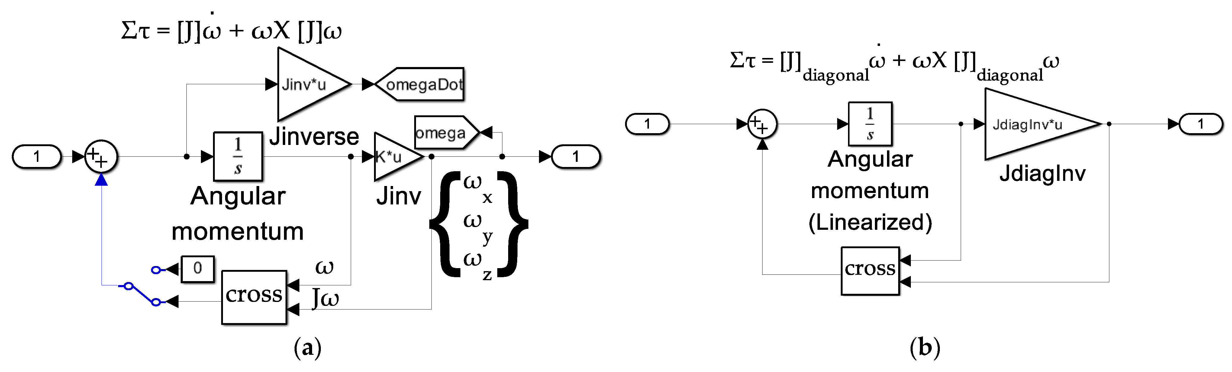
Figure A12.
Internal content of “Kinematics” subsystem depicted in Figure 3.
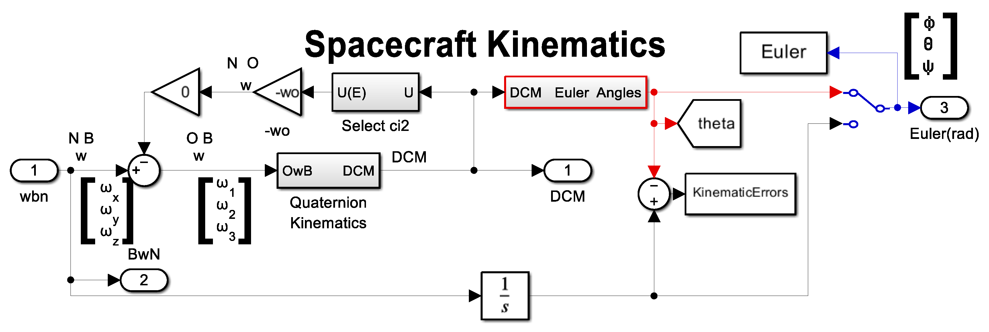
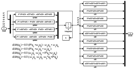
Figure A13.
Internal content of “Quaternion Kinematics” subsystem depicted in Figure A12.
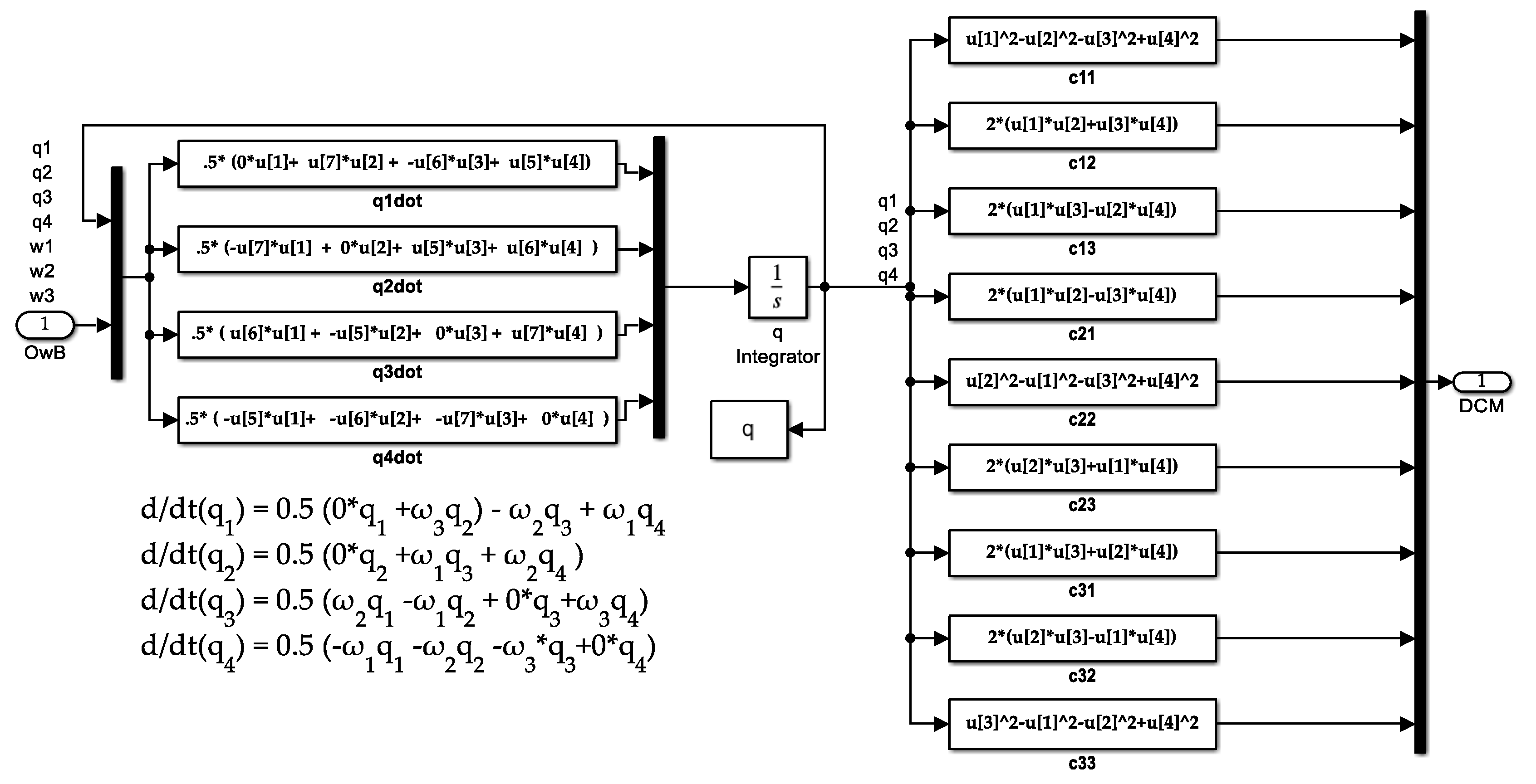
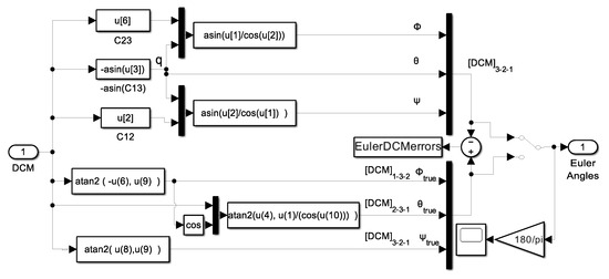
Figure A14.
Internal content of “DCM Euler Angles” subsystem depicted in Figure A12.
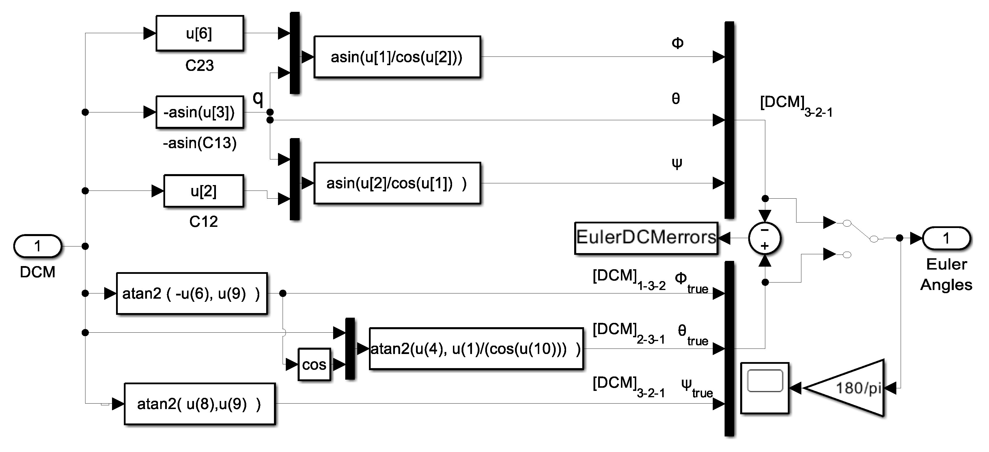
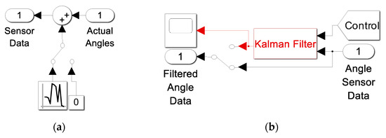
Figure A15.
Internal content of “Filters” subsystem and “Sensors” subsystems depicted in Figure 3 illustrated, respectively, in this figure’s (a,b).
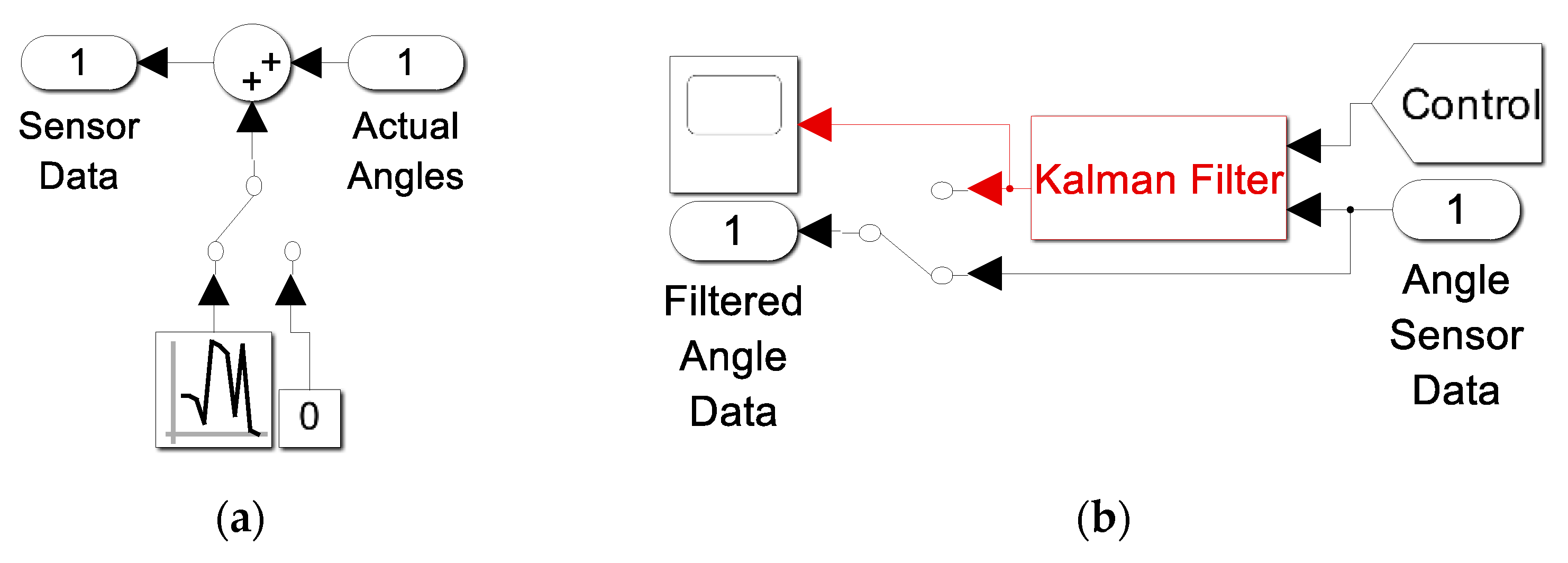

Figure A16.
High-level topology of environmental disturbances.
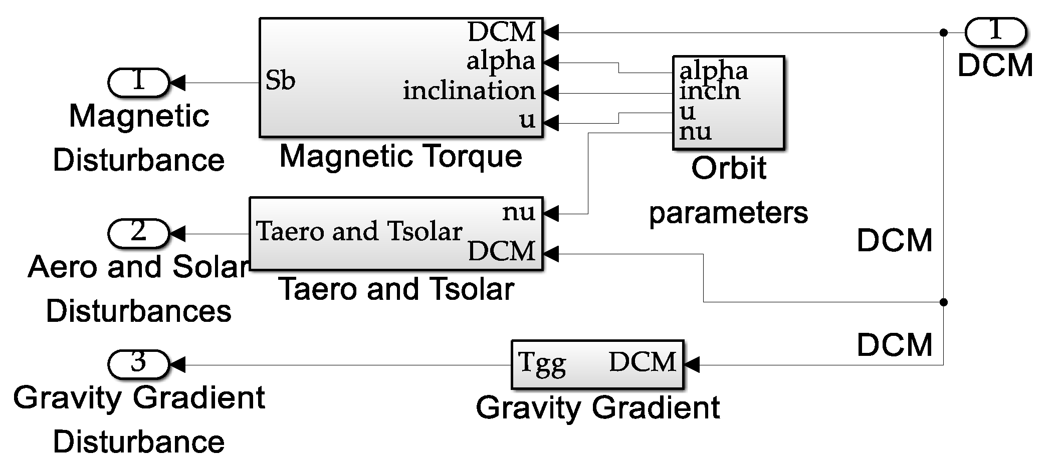
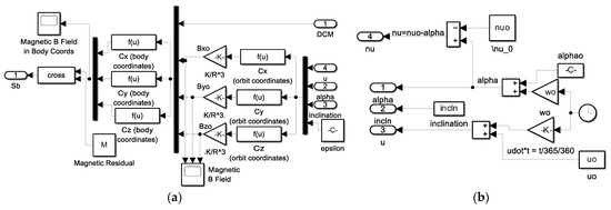
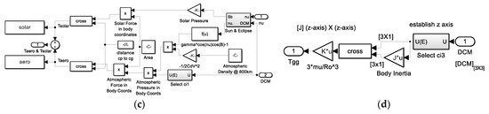
Figure A17.
Internal content of “Space Environment Disturbances” depicted in Figure A16 illustrated, respectively, in this figure’s (a–d): (a) subsystem labeled “Magnetic Torque” subsystem; (b) orbit parameters; (c) TAero and Tsolar; and (d) Gravity Gradient.

References
- Henshaw, C.; Glassner, S.; Naasz, B.; Roberts, B. Grappling Spacecraft. Annu. Rev. Control Robot. Auton. Syst. 2022, 5, 137–159. [Google Scholar]
- JPL Robotics. Available online: https://www-robotics.jpl.nasa.gov/what-we-do/research-tasks/prototype-grapple-arm-for-space-exploration-vehicle/ (accessed on 13 December 2024).
- PickNik Awarded NASA SBIR Phase 2 for In-Orbit Robot Autonomy. Available online: https://www.aerospacemanufacturinganddesign.com/news/picnik-robotics-awarded-nasa-sbir-phase-2-robot-autonomy/ (accessed on 18 November 2024).
- Robotic Refueling Mission 3 (RRM3). Available online: https://www.nasa.gov/nexis/robotic-refueling-mission-3/ (accessed on 18 November 2024).
- NASA Images and Media Usage Guidelines. NASA Content—Images, Audio, Video, and Media Files Used in the Rendition of 3-Dimensional Models, such as Texture Maps and Polygon Data in Any Format—Generally Are Not Subject to Copyright in the United States. Available online: https://www.nasa.gov/nasa-brand-center/images-and-media/ (accessed on 18 November 2024).
- Maclay, T.; Goff, J.; Sheehan, J.; Han, E. The development of commercially viable ADR services: Introduction of a small-satellite grappling interface. J. Space Saf. Eng. 2020, 3, 364–368. [Google Scholar]
- IEEE Robotics & Automation Society, Technical Committee for Space Robotics. Available online: https://www.ieee-ras.org/space-robotics (accessed on 18 November 2024).
- Hernández-Arias, H.; Prado-Molina, J. On-Orbit Center of Mass Relocation System for A 3U Cubesat. Int. J. Sci. Tech. Res. 2018, 7, 44–51. [Google Scholar]
- Calaon, R.; Kiner, L.; Allard, C.; Schaub, H. Momentum management of a spacecraft equipped with a dual—Gimballed electric thruster. In Proceedings of the AAS Guidance and Control Conference, Breckenridge, CO, USA, 2–8 February 2023. Paper No. AAS-23-178. [Google Scholar]
- Gracey, W. The experimental determination of the moments of inertia of airplanes by a simplified compound-pendulum method. Available online: https://ntrs.nasa.gov/citations/19930082299 (accessed on 25 March 2025).
- Soule, H.; Miller, M. The experimental determination of the moments of inertia of airplanes. Available online: https://ntrs.nasa.gov/citations/19930091541 (accessed on 25 March 2025).
- Genta, G.; Delpreta, C. Some considerations on the experimental determination of moments of inertia. Meccanica 1994, 29, 125–141. [Google Scholar]
- Nocerino, A.; Opromolla, R.; Fasano, G.; Grassi, M.; Balaguer, P.; John, S.; Cho, H.; Bevilacqua, R. Experimental validation of inertia parameters and attitude estimation of uncooperative space targets using solid state LIDAR. Acta Astronaut. 2023, 240, 428–436. [Google Scholar]
- Bourabah, D.; Field, L.; Botta, E. Estimation of uncooperative space debris inertial parameters after tether capture. Acta Astronaut. 2023, 202, 909–926. [Google Scholar] [CrossRef]
- Field, L.; Bourabah, D.; Botta, E. Online Control and Moment of Inertia Estimation of Tethered Debris. In Proceedings of the AIAA SCITECH 2024 Forum, Orlando, FL, USA, 8–12 January 2024. [Google Scholar]
- Sonobe, M.; Inoue, Y. Center of Mass Estimation Using a Force Platform and Inertial Sensors for Balance Evaluation in Quiet Standing. Sensors 2023, 23, 4933. [Google Scholar] [CrossRef]
- Zatsiorsky, V.M.; King, D.L. An algorithm for determining gravity line location from posturographic recordings. J. Biomech. 1997, 31, 161–164. [Google Scholar]
- Caron, O.; Faure, B.; Brenière, Y. Estimating the centre of gravity of the body on the basis of the centre of pressure in standing posture. J. Biomech. 1997, 30, 1169–1171. [Google Scholar]
- Germanotta, M.; Mileti, I.; Conforti, I.; Del Prete, Z.; Aprile, I.; Palermo, E. Estimation of Human Center of Mass Position through the Inertial Sensors-Based Methods in Postural Tasks: An Accuracy Evaluation. Sensors 2021, 21, 601. [Google Scholar] [CrossRef]
- Wang, F.; Bettadpur, S.; Save, H. Determination of the center–of–mass of gravity recovery and climate experimental satellites. J. Spacecr. Rockets 2010, 47, 371. [Google Scholar] [CrossRef]
- Kornfeld, R.; Arnold, B.; Gross, M.; Dahya, N.; Klipstein, W.; Gath, P.; Bettadpur, S. GRACE-FO: The Gravity Recovery and Climate Experiment Follow-On Mission. J. Spacecr. Rockets 2019, 56, 931–951. [Google Scholar] [CrossRef]
- Huang, Z.; Li, S.; Cai, L.; Fan, D.; Huang, L. Estimation of the Center of Mass of GRACE-Type Gravity Satellites. Remote Sens. 2022, 14, 4030. [Google Scholar] [CrossRef]
- Pan, Z.; Xiao, Y. Data Quality Assessment of Gravity Recovery and Climate Experiment Follow-On Accelerometer. Sensors 2024, 24, 4286. [Google Scholar] [CrossRef]
- Dou, Y.; Wang, K.; Zhou, Z.; Thomas, P.R.; Shao, Z.; Du, W. Investigation of the Free-Fall Dynamic Behavior of a Rectangular Wing with Variable Center of Mass Location and Variable Moment of Inertia. Aerospace 2023, 10, 458. [Google Scholar] [CrossRef]
- Geng, J.; Langelaan, J.W. Estimation of Inertial Properties for a Multilift Slung Load. J. Guid. Control Dyn. 2021, 2, 220–237. [Google Scholar] [CrossRef]
- Gahramanova, A. Locating Centers of Mass with Image Processing. Undergrad. J. Math. Model 2019, 10, 1. [Google Scholar] [CrossRef]
- Lin, Y.T.; Tian, Y.; Perez, D.; Livescu, D. Regression-Based Projection for Learning Mori–Zwanzig Operators. SIAM J. Appl. Dyn. Sys. 2023, 4, 2890–2926. [Google Scholar] [CrossRef]
- Setterfield, T.; Miller, D.; Leonard, J.; Saenz-Otero, A. Mapping and determining the center of mass of a rotating object using a moving observer. Int. J. Robot. Res. 2018, 37, 83–103. [Google Scholar] [CrossRef]
- Diagonalize the Inertia Tensor. Available online: https://phys.libretexts.org/Bookshelves/Classical_Mechanics/Variational_Principles_in_Classical_Mechanics_(Cline)/13%3A_Rigid-body_Rotation/13.07%3A_Diagonalize_the_Inertia_Tensor (accessed on 26 November 2024).
- Luenberger Observer. Available online: https://www.mathworks.com/help/sps/ref/luenbergerobserver.html (accessed on 19 November 2024).
- Transport Theorem. Available online: https://en.wikipedia.org/wiki/Transport_theorem (accessed on 19 November 2024).
- Fossen, T. Comments on ‘Hamiltonian adaptive control of spacecraft’. IEEE Trans. Autom. Control 1993, 38, 671–672. [Google Scholar] [CrossRef]
- Iven, M.; Mareels, B.; Anderson, R.; Bitmead, R.; Bodson, M.; Sastry, S. Revisiting the MIT rule for adaptive control. In Adaptive Systems in Control and Signal Processing 1986; IFAC Workshop Series; Pergamon Press Ltd.: Oxford, UK, 1987; pp. 161–166. [Google Scholar]
- Kuck, E.; Sands, T. Space Robot Sensor Noise Amelioration Using Trajectory Shaping. Sensors 2024, 24, 666. [Google Scholar] [CrossRef] [PubMed]
- Adams, G. Arizona State University Physics Department Proof of the Parallel Axis Theorem. Available online: https://www.public.asu.edu/~gbadams/sum00/parallelaxisT.pdf (accessed on 19 November 2024).
- Zhu, Y. Identification Test Design and Data Pretreatment. In Multivariable System Identification for Process Control; Zhu, Y., Ed.; Elsevier Science: Maryland Heights, MO, USA, 2001; pp. 31–63. [Google Scholar]
- Persistent Excitation Conditions and Their Implications. Section 8.1 of Study Guide on Adaptive and Self-Tuning Control. Available online: https://library.fiveable.me/adaptive-and-self-tuning-control/unit-8/robustness-issues-adaptive-control/study-guide/yLKsaWxBlamk2I48 (accessed on 22 November 2024).
- Marino, R.; Tomei, P. On exponentially convergent parameter estimation with lack of persistency of excitation. Syst. Control Lett. 2022, 159, 105080. [Google Scholar]
- Korotina, M.; Romero, J.; Aranovskiy, S.; Bobtsov, A.; Ortega, R. A new on-line exponential parameter estimator without persistent excitation. Syst. Control Lett. 2022, 159, 105079. [Google Scholar]
- Software, Robotics, and Simulation Division. Available online: https://www.nasa.gov/software-robotics-and-simulation-division/ (accessed on 21 November 2024).
- Dynamics Operations Training Systems. Available online: https://www.nasa.gov/general/generic-robotics-on-orbit-trainer/ (accessed on 21 November 2024).
- Dai, Q.; Xiao, G.; Zhou, G.; Ye, Q.; Han, S. A novel Gaussian sum quaternion constrained cubature Kalman filter algorithm for GNSS/SINS integrated attitude determination and positioning system. Front. Neurorobotics 2024, 18, 1374531. [Google Scholar]
- Slotine, J.; Di Benedetto, M. Hamiltonian adaptive control of spacecraft. IEEE Trans. Autom. Control 1990, 35, 848–852. [Google Scholar] [CrossRef]
- Sands, T.; Kim, J.; Agrawal, B. Improved Hamiltonian Adaptive Control of spacecraft. In Proceedings of the IEEE Aerospace conference, Big Sky, MT, USA, 7–14 March 2009. [Google Scholar]
- Sands, T.; Kim, J.; Agrawal, B. Spacecraft fine tracking pointing using adaptive control. In Proceedings of the 58th International Astronautical Congress, Hyderabad, India, 24–28 September 2007. [Google Scholar]
- Sands, T.; Kim, J.; Agrawal, B. Spacecraft adaptive control evaluation. In Proceedings of the Infotech@Aerospace, Garden Grove, CA, USA, 19–21 June 2012. [Google Scholar]
- Huang, B.; Sands, T. Novel learning for control of nonlinear spacecraft dynamics. J. AppliedMath 2023, 1, 42. [Google Scholar] [CrossRef]


Disclaimer/Publisher’s Note: The statements, opinions and data contained in all publications are solely those of the individual author(s) and contributor(s) and not of MDPI and/or the editor(s). MDPI and/or the editor(s) disclaim responsibility for any injury to people or property resulting from any ideas, methods, instructions or products referred to in the content. |
© 2025 by the author. Licensee MDPI, Basel, Switzerland. This article is an open access article distributed under the terms and conditions of the Creative Commons Attribution (CC BY) license (https://creativecommons.org/licenses/by/4.0/).