Abstract
Worldwide, heart disease is the leading cause of mortality. Cardiac auscultation, when conducted by a trained professional, is a non-invasive, cost-effective, and readily available method for the initial assessment of cardiac health. Automated heart sound analysis offers a promising and accessible approach to supporting cardiac diagnosis. This work introduces a novel method for classifying heart sounds as normal or abnormal by leveraging time-frequency representations. Our approach combines three distinct time-frequency representations—short-time Fourier transform (STFT), mel-scale spectrogram, and wavelet synchrosqueezed transform (WSST)—to create images that enhance classification performance. These images are used to train five convolutional neural networks (CNNs): AlexNet, VGG-16, ResNet50, a CNN specialized in STFT images, and our proposed CNN model. The method was trained and tested using three public heart sound datasets: PhysioNet/CinC Challenge 2016, CirCor DigiScope Phonocardiogram Dataset 2022, and another open database. While individual representations achieve maximum accuracy of ≈85.9%, combining STFT, mel, and WSST boosts accuracy to ≈99%. By integrating complementary time-frequency features, our approach demonstrates robust heart sound analysis, achieving consistent classification performance across diverse CNN architectures, thus ensuring reliability and generalizability.
1. Introduction
According to the Organization for Economic Cooperation and Development (OECD), the economic impact of cardiovascular diseases and diabetes poses a risk to the future development and public health sustainability of developing countries [1]. Worldwide, cardiovascular diseases are the leading cause of morbidity and mortality, with an estimation of 20 million people dying annually from cardiovascular-related diseases in recent years, representing approximately one-third of all deaths by noncommunicable diseases worldwide [2]. If adequately performed by a trained physician, cardiac auscultation can opportunely diagnose cardiovascular diseases (CVDs) at a low cost [3]. Modern digital stethoscopes allow the acquisition of heart sounds, also known as phonocardiogram (PCG) signals, with relatively good quality and simplicity. Recently, a push for the development of computer-aided diagnosis (CAD) systems based on PCG signals is underway, insomuch as these signals reflect the mechanics of the heartbeat (HB) [4].
Generally, a healthy phonocardiogram signal consists of two fundamental heart sounds called S1 and S2. These sounds are generated during the cardiac cycle (CC) by the closure of the atrioventricular and semilunar valves, respectively [4]. The CC exhibits a quasi-periodic behavior, formed by the systole (contraction), marking the beginning of S1; and by the diastole (relaxation), marking the beginning of S2. These sounds only represent a fraction of each of the CC sections, so there are two moments of quiet in healthy persons: the systolic (s-Sys) and the diastolic silences (s-Dia). In most cases, individuals with heart pathologies present additional sounds, such as the S3 and S4 sounds, murmurs, frictions, or clicks.
The PCG is a nonstationary signal, i.e., a signal whose properties and statistics change as a function of time. The diastole interval is usually longer than the systole interval. The S1 and S2 heart sounds usually have a duration between 25 and 150 ms, and their spectral content is mainly in the range from 24 to 144 Hz [5]. In the case of pathologies (clicks, frictions, and murmurs), their duration varies considerably within the cardiac cycle, and their spectral content is in the range from 25 Hz up to 700 Hz [6].
Accurately identifying sounds related to heart valve disorders can contribute to marking cardiac events of clinical relevance. Ideally, early detection can help reduce the mortality caused by cardiovascular diseases. Computer-aided diagnosis can help detect sounds automatically and differentiate between murmurs of potential pathological conditions. In recent years, supervised learning-based approaches have successfully classified cardiac sounds. Many machine-learning-based heart sound analysis and classification techniques have been proposed. An in-depth review of the literature in PCG analysis is beyond the scope of this paper, but a thorough assessment of past and recent techniques can be found in [7,8,9]. As shown in Figure 1, the automatic analysis and classification of PCG signals can be considered as composed of four main stages: (1) signal denoising and preprocessing, (2) segmentation, (3) feature extraction and dimensionality reduction, and (4) classification of the selected features. PCG signals are often corrupted by noise from breathing, body sounds, microphone friction, and ambient sources. While noise removal is ideal, current methods mainly preprocess raw data for analysis. PCG segmentation focuses on identifying key heart sounds (S1, S2) and the systolic/diastolic phases. Many classification algorithms use segmentation to pinpoint where to extract relevant features, simplifying further processing [10,11]. However, other PCG analysis algorithms skip the segmentation altogether and proceed directly to the feature extraction stage [12,13].
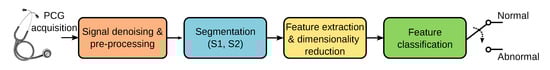
Figure 1.
Stages involved in the automatic classification of PCG signals.
Perhaps the most common technique for feature extraction is converting the PCG time waveform to different domains using specialized transforms. Combining multiple feature types is a common technique in PCG classification, often using transformations like the Fourier transform [14,15,16], or constant-Q transform [17]. Time-frequency representations (TFRs) such as the short-time Fourier transform (STFT) [18,19,20,21] have been used. Some approaches use features obtained from quadratic time-frequency distributions such as Wigner-Ville [22,23] or Choi-Williams [24,25]. One of the most widely used methods to generate features is the wavelet transform, and wavelet packets [13,26,27,28,29,30,31]. Another prevalent method to generate features, particularly in speech recognition, are the mel-frequency cepstral coefficients (MFCCs). The top three ranked algorithms in the Classification of Heart Sound Recordings: The PhysioNet/Computing in Cardiology Challenge 2016 competition [32] use MFCCs as features [33,34,35], but also other more recent approaches [17]. Other related versions exist, such as the mel-scale wavelet transform [36]. Sparse representations of PCG signals have also been proposed as features since they allow the representation of complex data in a low-dimensional space [37,38,39]. Empirical mode decomposition is a related method to the sparse representations of signals, where a few intrinsic mode functions can be used to represent the PCG [13,40]. Multi-domain low-level audio features such as energy in different subbands, high-order statistics, entropy, and zero-crossing rate, among others, have also been proposed [41,42,43].
The final step in heart sound classification involves feeding features into a classifier. Early methods relied on traditional machine learning, but recent approaches favor deep learning. Both achieve high performance, but deep learning requires less human intervention, as it automatically extracts features from signal representations and learns from errors. However, it demands more memory and computational power, often requiring GPUs. Among the traditional classifiers used in PCG analysis are support vector machines (SVM) [6,30,42,44,45,46], hidden Markov models (HMM) [27,47,48], random forest (RF) [30,38], k-nearest neighbor (KNN) [18,49] and artificial neural networks (ANN) [15,33,34,35]. Among the deep-learning classifiers, the most commonly used are convolutional neural networks (CNN) [21,46,50,51,52], but long-short memory neural networks (LSTM-NN) [53,54], variational autoencoder neural networks [55,56], and vision transformers (ViT) [57] have also been proposed.
In this work, we propose a new offline method combining three time-frequency representations to precisely describe the PCG as an image. Then we present how to accurately classify these images using well-established high-performance deep-learning architectures. Using three public heart sound recording datasets, the proposed methodology achieves 99.9% accuracy in detecting abnormal sounds. The rest of the paper is organized as follows. Section 2 presents the databases used in this study, the preprocessing steps, and the details on generating PCG images using time-frequency representations. This section also presents the image classification approach based on five deep-learning architectures. The results are reported and discussed in Section 3. Finally, concluding remarks are presented in Section 4.
2. Methodology
The structure of our PCG classification algorithm consists of three main stages: (1) preprocessing, (2) time-frequency analysis, and (3) machine-learning classification. A detailed description of each of these steps is presented in this section.
2.1. Heartsound Datasets
We propose using three publicly available heart sound databases for this work’s development. The first database is used in “The PhysioNet/Computation in Cardiology (CinC) Challenge 2016” [58]. This collection of sounds comes from seven independent research groups. The database contains 3153 heart sound recordings collected from healthy patients and patients with different cardiac pathologies, such as heart valve disease and coronary artery disease, among others. The database composition is presented in Table 1, the letters A, …, F refer to each of the research groups that contributed to the database; details are provided in [58]. This dataset exhibits class imbalance, predominating normal sounds over abnormal ones.

Table 1.
Conformation of the PCG recordings in the PhysioNet dataset [58].
The second database we used is “The George B. Moody PhysioNet Challenge 2022” [59]. This dataset contains 5272 heart sound recordings collected from 1568 subjects. The target population was individuals who were 21 years old or younger. A detailed description of the database is presented in [60], but it mainly consists of heart sounds from aortic, pulmonary, tricuspid, and mitral locations that were recorded from healthy and pathological subjects with heart valve and coronary artery diseases. Each cardiac murmur has been manually annotated by an expert annotator according to its timing, shape, pitch, grading, and quality. Recordings were made in clinical and non-clinical settings and are classified as normal, abnormal, or unsure. The sounds labeled as unsure were not considered in this study. In addition, the dataset is unbalanced, with more recordings corresponding to normal than abnormal sounds.
The third database we used is the one assembled by [61]. It contains one thousand heart sound recordings, and it is composed of both abnormal and normal sounds. It contains 800 pathological sounds, which are uniformly divided into four categories corresponding to the following diseases: aortic stenosis (AS), mitral stenosis (MS), mitral regurgitation (MR), and mitral valve prolapse (MVP). The database composition is presented in Table 2.
Table 2.
Conformation of the PCG dataset assembled by Yaseen et al. [61]. The abnormal or pathological sounds are divided into four classes corresponding to the following diseases: aortic stenosis (AS), mitral stenosis (MS), mitral regurgitation (MR), and mitral valve prolapse (MVP).
2.2. Preprocessing
Initially, the sounds in these databases have been digitized using different sampling rates and 16-bit resolution. For the present work, the signals were resampled, and the sampling frequency was set to Hz with 16-bit resolution. Then the signals were filtered using a Butterworth band-pass filter with cutoff frequencies of 25 Hz and 900 Hz.
This work did not consider sounds from the PhysioNet database marked as unfit for classification since these recordings correspond to highly noisy signals.
2.3. Time-Frequency Analysis
One of the most exploited properties in digital signal analysis is the time-frequency duality inherent to signals since the representation of a signal in one of these domains will provide different and complementary information about the same signal in the other domain. However, the information in the original signal domain is lost once the transformation occurs. Time-frequency analysis makes it possible to conserve the information in both domains and to characterize signals whose statistics vary simultaneously in time and frequency. In the present work, we use three time-frequency representations: (1) the short-time Fourier transform, (2) the mel spectrogram, and (3) the wavelet synchrosqueezed transform. As mentioned earlier, the use of time-frequency analysis has been previously proposed in the context of PCG signal classification; however, we are unaware of prior work adopting a similar approach of combining in a single image different representations.
2.3.1. Short-Time Fourier Transform
The short-time Fourier transform (STFT) is probably the most commonly used time-frequency representation. The main reasons behind the STFT popularity are its simplicity, computational speed, and highly satisfactory performance. The calculation principle of the STFT is the translation and modulation of a window function [62]. A real and symmetric window is translated in time by and modulated by the frequency : , where for any . The resulting windowed Fourier transform for a PCG signal is then
the STFT localizes the energy of the Fourier integral in the neighborhood of [62]. In practice, the PCG recordings we want to analyze are discrete-time, and the data to be transformed are divided into blocks or frames and processed using the discrete STFT. For each block, the discrete Fourier transform (DFT) is calculated, and the result is a complex vector that is added as a column to a matrix, which records the magnitude and phase of each point in time and frequency. The discrete STFT is computed as follows [63]:
where is a window function of length samples; n is the discrete time index; m is a new time (frame) index; R is the hop size between two consecutive time frames m and , with , where M is the total number of STFT frames. In practice, the fast Fourier transform (FFT) is used to compute the DFT. The set of frequency bins is defined as , for where N is the DFT length. Finally, is the sampling frequency of the PCG, and is the sampling frequency of the new time vector m. The STFT is a complex-valued 2D function. In the present work, we are only interested in the energy density as a function of time and frequency; for this reason, the STFT image that we use is obtained by , which is usually known as the spectrogram.
The STFT implementation parameters used in our proposal are as follows: PCG blocks of samples were processed using a Hamming-type analysis window of length samples, an overlap of samples and the FFT length of samples. Using these parameters, the spectrogram has a size of 257 × 224. Since the CNN architectures we have decided to use in this work require an input image of different dimensions than those of , the spectrogram was cropped to fit the size 224 × 224. In this case, rows 225 to 257 were removed, i.e., the subsequent PCG analysis only considers frequencies of up to ≈871 Hz. We consider it safe to discard that frequency range since it hardly contains any PCG energy. Figure 2a,b illustrate the cropped spectrograms and the type of images that we use; these correspond to the PCG waveforms presented in Figure 3. The advantage of converting a PCG signal block of 1.4 s (2800 samples) to an image is that cardiac signal segmentation is not required. In practice, we can be sure that the block under analysis contains at least one entire cardiac cycle. The overlap between contiguous PCG blocks is 1400 samples.
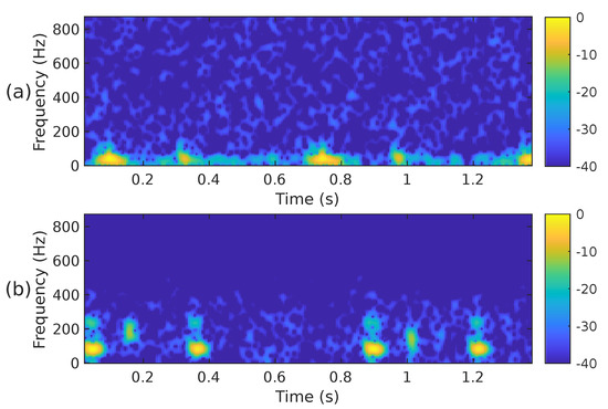
Figure 2.
The spectrogram, i.e., , of the two PCG signals presented in Figure 3: (a) corresponds to a healthy person, while (b) corresponds to an abnormal heart sound.
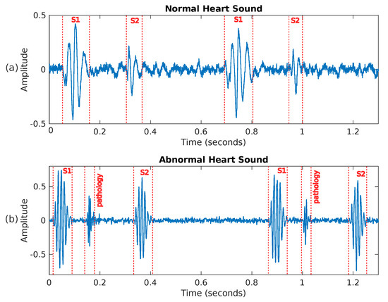
Figure 3.
Two examples of heart sounds: (a) shows a PCG signal corresponding to a healthy person, while (b) presents an abnormal PCG signal where a pathology is visible between sounds S1 and S2.
2.3.2. Mel Spectrogram
It has been known for decades that humans do not perceive frequencies on a linear scale; detecting changes in lower frequencies is easier than distinguishing them in higher frequencies. The mel scale is an attempt to measure pitch’s psychological sensation such that equal distances in pitch sounded equally distant to a listener [64]. The reference point between the mel scale and the linear frequency scale in Hertz is defined arbitrarily by equating a 1000 Hz tone, 40 dB above the listener’s hearing threshold, with a 1000 mels tone. The mel and the linear frequency scale are related by . According to the mel scale, the mel spectrogram can be considered a rescaled spectrogram in its vertical axis. In practice, the rescaling operation uses a set of band-pass filters, specifically a half-overlapped triangular set of filters equally spaced on the mel scale. Figure 4 shows the filter bank used in this work; we decided to use bands, as proposed in [65] for PCG signals sampled at 2 kHz. The mel spectrogram values are obtained by multiplying the frequency domain values (i.e., the FFT bins) of the columns of by the corresponding matrix composed of triangular filters and then adding the result. This process is repeated for the M STFT frames. More specifically, let be the array that contains the mel-scale filterbank, where and . The mel spectrogram is obtained by computing the expression
where ℓ is the mel-frequency band index and m is the time-frame index. Figure 5 shows the mel spectrogram corresponding to the PCG waveforms presented in Figure 3. Both mel spectrograms closely resemble the linear spectrograms of Figure 2, but with less detail.
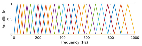
Figure 4.
In In the present work, we use a set of 24 half-overlapped triangular filters equally spaced on the mel scale. The line colors have been added to more easily differentiate each filter band.
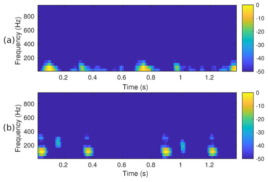
Figure 5.
The mel spectrogram, i.e., , of the two PCG signals presented in Figure 3: (a) corresponds to a healthy person, while (b) corresponds to an abnormal heart sound.
2.3.3. Synchrosqueezed Wavelet Transform
The wavelet synchrosqueezed transform (WSST) [66] is a relatively recent and highly effective time-frequency analysis technique for examining non-stationary signals with many oscillating modes. As with most sound signals, the PCG can be accurately expressed as the sum of amplitude and frequency-modulated components [67]. Similarly to other linear time-frequency methods, the basic wavelet transform (WT) breaks down the signal under analysis into its components by correlating it with a dictionary of time-frequency atoms [62]. The wavelet transform is based on the principle of translating and contracting/dilating copies (i.e., atoms) of a basic fast-decaying oscillating waveform , known as the mother wavelet. The wavelet is a normalized function , centered around and with zero average, that is, . The definition of the continuous wavelet transform (CWT) of the signal is as follows:
where the family of time-frequency atoms is obtained by translating by u and scaling it by s such that the atom remains normalized, where and * is the complex conjugate. A drawback of the WT, but also many other TFRs, is the time-frequency energy spreading associated with the atoms, which negatively impacts the sharpness of the signal under analysis [62,66]. A consequence of this spread is that it permits a non-zero amplitude to be obtained even though the original signal does not have a component at the given time-frequency pair. To overcome this limitation, the concept of synchrosqueezing transformation (SST) has been proposed [66,68]; this technique enhances the representations by reassigning the local signal energy in the frequency domain. The reassignment compensates for the spreading effects caused by the mother wavelet. In contrast to other time-frequency reassignment techniques, synchrosqueezing reassigns energy exclusively in the frequency direction, maintaining the signal’s temporal resolution. By preserving the time, the inverse WSST allows the reconstruction of the original signal. The steps to obtain the WSST [66] start with the calculation of the CWT as indicated by Equation (4). The CWT must use an analytic wavelet to capture instantaneous frequency information. In this work, we use the analytic Morlet wavelet, also known as the Gabor wavelet, which consists of a Gaussian window modulated by a complex exponential. The non-analytical wavelet with , where are the modulated Gaussian window’s center frequency and variance, respectively [62,69]. The analytical wavelet is obtained by computing the Hilbert transform of . The analytic Morlet wavelet is defined in the Fourier domain by
where if and ; otherwise, that is, the frequency domain unit step function. To compute the CWT, the next step is to extract the instantaneous frequencies from using the following phase transform, , that is proportional to the first derivative of the CWT with respect to the translation u
The smeared energy is then relocated to the instantaneous frequencies to synchrosqueeze the time-frequency representation. This compression is conducted by relocating the energy at the points . We obtain the SST representation by computing
when mapping the time-scale plane to the time-frequency plane the transformation is calculated only at discrete central frequencies separated by a frequency step . Since are discrete variables in practice, a scaling step is introduced, separating the scales for which the is calculated. A thorough explanation of the calculation of the WSST is provided in [66,68]. Although it has been reported that the energy of cardiac sounds is below 700 Hz [6], their spectral content above 500 Hz is practically negligible. According to [4], sounds recorded from the chest wall in the 500–1000 Hz range have significantly reduced amplitude. This low amplitude, rather than the human hearing threshold, is the primary reason for their limited or absent audibility. For this reason and to reduce the computational complexity of the WSST, the PCG input signal was resampled to a frequency of 1000 Hz. In addition, the transformation was computed for a block of 1400 samples at 224 different scales ranging from ≈6 Hz up to 500 Hz. Figure 6 shows the WSST corresponding to the PCG waveforms presented in Figure 3. The figure shows how using the SST leads to an improved resolution and sharpness as compared to the STFT and mel spectrogram.
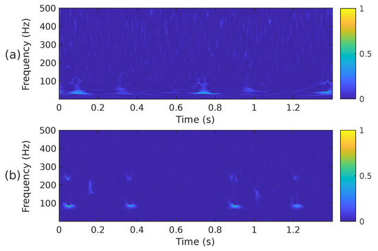
Figure 6.
The WSST, i.e., , of the two PCG signals presented in Figure 3, (a) corresponds to a healthy person, while (b) corresponds to an abnormal heart sound.
2.3.4. Combination of Time-Frequency Representations
Choosing the most appropriate features for PCG classification has been a challenging problem for many years. The performance results obtained in other sound classification applications often influence the selection of features in PCG analysis. It has also been documented that, in general, the combination of several feature extraction methods exhibits better performance than a single type of feature [7]. Based on this premise, we have combined the previously introduced time-frequency representations in the following ways. First, we have combined the STFT, the mel spectrogram, and the WSST in a single image. These representations have been cropped to fit into a matrix, from bottom to top, in the following way. For the WSST, the frequency range from ≈25 Hz up to ≈363 Hz () was kept; for the STFT, the frequency range from 0 Hz up to ≈325 Hz () was kept; and for the mel spectrogram, the whole representation, 0 Hz up to 1000 Hz, () was considered. The resulting time-frequency representation is shown in Figure 7a,b, corresponding to the PCG waveforms in Figure 3. In the second case, we combined the WSST in the frequency range from ≈25 Hz up to ≈363 Hz (), and the STFT in the range from 0 Hz up to ≈422 Hz (). The resulting time-frequency representation is shown in Figure 8. In the third case, we combined the WSST in the frequency range from ≈1 Hz up to 500 Hz (), and for the mel spectrogram in the range 0 Hz up to 1000 Hz (), as shown in Figure 9. In the fourth case, we combined the STFT in the frequency range from 0 Hz up to ≈777 Hz (), and the mel spectrogram in the range 0 Hz up to 1000 Hz (), as shown in Figure 10.
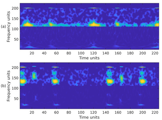
Figure 7.
Combination of the cropped time-frequency representations WSST + STFT + MEL of the two PCG signals presented in Figure 3: (a) corresponds to a healthy person, while (b) corresponds to an abnormal heart sound. The horizontal and vertical axes have been adjusted to the size .
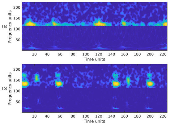
Figure 8.
Combination of the cropped time-frequency representations WSST + STFT of the two PCG signals presented in Figure 3: (a) corresponds to a healthy person, while (b) corresponds to an abnormal heart sound. The horizontal and vertical axes have been adjusted to the size .
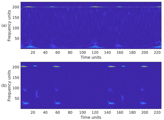
Figure 9.
Combination of the cropped time-frequency representations WSST + MEL of the two PCG signals presented in Figure 3: (a) corresponds to a healthy person, while (b) corresponds to an abnormal heart sound. The horizontal and vertical axes have been adjusted to the size .
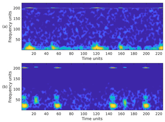
Figure 10.
Combination of the cropped time-frequency representations STFT + MEL of the two PCG signals presented in Figure 3: (a) corresponds to a healthy person, while (b) corresponds to an abnormal heart sound. The horizontal and vertical axes have been adjusted to the size .
Since the classification algorithms use an input image of size , the time-frequency representation that only includes the mel spectrogram was not considered since its size is . In total, the following six variants of time-frequency representations are considered in the rest of this work: (1) STFT, (2) WSST, (3) WSST + STFT + mel, (4) WSST + STFT, (5) WSST + mel, (6) STFT + mel.
2.4. Machine-Learning Classifiers
Section 1 explained that the final step in PCG analysis involves feeding extracted features into a classifier to determine whether the signal is normal or abnormal. Two main types of classifiers are commonly used: (1) traditional machine-learning (e.g., KNN, SVM, RF) and (2) deep-learning algorithms (e.g., CNNs, ViT). Recently, hybrid methods combining both approaches have been proposed [46]. This work employs deep-learning algorithms based on CNNs.
Deep-learning methods use multi-level representations by transforming data through simple, non-linear modules, progressing from low-level to higher, more abstract features. These high-level representations emphasize relevant input aspects for classification tasks while suppressing irrelevant ones [70].
Convolutional layers are the core of CNNs. A convolution applies a filter to the input, producing a feature map that highlights the location and magnitude of detected features. CNNs innovate by learning multiple parallel filters tailored to the problem, enabling the detection of specific dataset features. Convolution involves a linear operation where a filter (or kernel), smaller than the input, is systematically applied across the input data. This operation computes a dot product between the filter and corresponding input sections, moving from left to right and top to bottom [71]. This process, known as translation invariance, focuses on the presence of features rather than their position. The resulting filtered values form a two-dimensional feature map [71,72].
This work evaluates five CNN architectures for classifying PCG signals, each with unique attributes. First, we use two classical networks: AlexNet [73] and VGG-16 [74]. These networks may suffer from the exploding and vanishing gradient problem, leading to increased error rates and potential overfitting. To address this, we include ResNet50 [75], which uses skip connections to bypass layers, enabling deeper architectures and learning more complex features.
We also evaluate the CNN proposed by Ullah et al. [76], designed for spectrogram images of ECG signals. This network has fewer parameters and achieves high performance with low computational cost. Lastly, we propose a custom CNN designed for PCG time-frequency representations, as shown in Figure 11. Creating a custom CNN for PCG signal classification using time-frequency representations proved challenging given our current deep-learning expertise. We aimed to replicate effective architectures while reducing computational demands. Despite achieving high performance (see Section 3), we acknowledge that we require greater expertise to create a more resource-efficient solution.
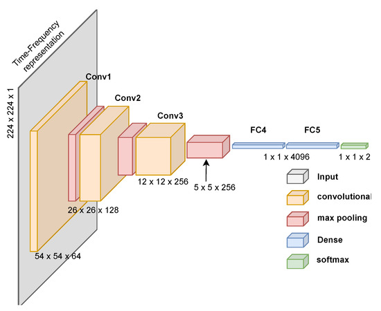
Figure 11.
Proposed CNN architecture to classify time-frequency images generated from PCG signals. The architecture includes the processing dimensions through each layer.
The rationale for using different architectures is to provide a more complete evaluation of the classification capabilities to identify abnormal PCG signals. These networks represent different CNN generations, each suited to specific image classification tasks.
The first three CNN architectures were designed to classify hundreds of different types of images and use a three-channel input matrix to account for the colors (typically red, green, and blue). Images created from the time-frequency representations of heart sounds have only one channel. For this reason, it was necessary to slightly modify the networks in the input and output layers. Specifically, the input layer was adapted to receive images of size 224 × 224 × 1, and in the output layer, it was modified only to have two possible results: a prediction of whether the input image corresponds to an abnormal or normal sound.
Image Data Generation and Network Implementation
After following the methodology described in Section 2.3 and using the three datasets described in Section 2.1, 17,200 images are generated using each of the six time-frequency variants. That is, in total, 103,200 images were created and processed by the five CNN architectures. The images were balanced in a 1:1 ratio between TFRs generated from normal and abnormal sounds. Specifically, for each type of TFR, 8600 images are labeled as “pathological”, and 8600 images are labeled as “healthy”. Balanced classes in machine learning prevent biased models from favoring the majority class [77]. To address the class imbalance, we randomly undersampled the normal PCG sounds to match the number of abnormal sounds, ensuring a balanced dataset for analysis. The publicly available datasets used in this study comprise independent recordings from various laboratories globally, each employing distinct recording equipment and protocols. While this inherent heterogeneity could lead to some recordings from the same individual being present in different cross-validation folds, it also mitigates the risk of overfitting to a particular recording setup or patient demographic. To further reduce potential bias, we implemented balanced undersampling, maintaining a proportional representation of samples from each source laboratory across all folds. MATLAB R2022b was used to program the signal-processing part of the algorithm. Python v3.11.4 was used to program the classification part of the algorithm. The CNNs were implemented using the TensorFlow and Keras AI libraries. The networks were trained using the paid version of Google Collaboratory. The hyperparameters used to train the networks are the following:
- optimizer: stochastic gradient descent (SGD),
- learning rate: 0.0008
- loss function: categorical cross-entropy,
- batch size: 64 samples
- training: 150 epochs or less (depending on the test’s error rate, an early stop was implemented).
Section 3 presents the result of the 10-fold cross-validation. In each fold, of the 10,200 images, 90% (9180 images) were randomly selected for training and the remaining 10% (1020 images) for validation.
3. Results
3.1. Performance Metrics
The confusion matrix is a fundamental performance measurement in machine learning. This matrix allows the comparison of the algorithm-predicted and actual values for two or more classes. In our case, the two output classes indicate whether the PCG signal is “normal” or “abnormal”. This situation has four probable outcomes:
- 1.
- True positive (TP) indicates the number of diseased PCGs the classifier correctly predicts as diseased.
- 2.
- False positive (FP) represents the number of diseased PCGs that the classifier wrongly predicts as being healthy.
- 3.
- True negative (TN), shows how many times the real and predicted values are both considered to be healthy (i.e., normal).
- 4.
- False positive (FP) shows how many times the classifier incorrectly predicted the PCG as diseased when it is not.
We used five metrics to assess the performance of the proposed methodology: accuracy, sensitivity, specificity, precision, and F1-score [78]. Accuracy refers to how close the result of a measurement is to the true value. It is represented as the ratio of the number of correct predictions to the total number in the dataset.
Sensitivity, also called true positive rate, refers to the ability of the algorithm to classify positive cases; it is calculated using Equation (9). The best sensitivity value is 1; the worst is 0.
Specificity, also called true negative rate, refers to the ability of the algorithm to classify negative cases; it is calculated using Equation (10). The best specificity value is 1; the worst is 0.
Precision refers to the dispersion of the set of values obtained from repeated measurements of a magnitude. It is represented as the ratio between the number of true predictions and the total number of true predictions; it is calculated using Equation (11). The best precision value is 1; the worst is 0.
F1-score is a metric that summarizes the forecast and sensitivity in a result; it is calculated using Equation (12).
3.2. Experimental Results
The experimental results obtained after combining the six time-frequency representations and the five deep-learning architectures are presented below. In the following tables, the naming convention for the six time–frequency representations are the following: (1) S stands for STFT, (2) M stands for STFT + mel, (3) W stands for WSST, (4) WSM stands for WSST + STFT + mel, (5) WS stands for WSST + STFT, and (6) WM stands for WSST + mel.
Table 3 presents the performance results for the AlexNet architecture. It can be seen that among the single time-frequency representations, with an accuracy of 85.89%, the STFT exhibits a slightly better performance than the STFT + mel and a notably better performance than the WSST. This last result was unexpected since the WSST provides an enhanced and more precise representation of the PCG signal’s time-varying frequency and amplitude components. Another surprising result was obtained when two or more time-frequency representations were combined since the performance significantly improved, particularly for the WSST + STFT + mel and WSST + STFT combinations that exhibit an accuracy of 99.96% and 99.95%, respectively.
Table 3.
PCG classification performance comparison between time-frequency representations using the AlexNet CNN architecture. The table presents the mean of a 10-fold cross-validation.
Table 4 presents the performance results for the VGG-16 architecture. This network presents a similar behavior as AlexNet; however, the performance for the single time-frequency representations is considerably lower, with an accuracy of ≈75%. The performance boost for the WSST + STFT + mel, and WSST+STFT combinations is remarkable, almost reaching 99%, but the performance is slightly lower than the performance obtained by AlexNet. The WSST + mel also showed a substantial improvement, but not nearly as prominent as the other two combinations.
Table 4.
PCG classification performance comparison between time-frequency representations using the VGG-16 CNN architecture. The table presents the mean of a 10-fold cross-validation.
Table 5 presents the performance results for Ullah et al., [76] architecture. This CNN presents a comparable behavior to both previously presented architectures; however, the performance for the single time-frequency representations is poor. The performance boost for the WSST + STFT + mel and WSST + STFT combinations is again remarkable, surpassing VGG-16, but performance is slightly lower than AlexNet. The WSST + mel also showed poor performance.
Table 5.
PCG classification performance comparison between time-frequency representations using the Ullah et al., [76] CNN architecture. The table presents the mean of a 10-fold cross-validation.
Table 6 presents the performance results for our architecture proposal; see Figure 11. This CNN presents a comparable behavior to the previous architectures, particularly AlexNet. The performance for the single time-frequency representations is lower than AlexNet but higher than the other analyzed networks. Again, the performance boost for the combination of representations is remarkable, but this time the WSST + mel combination also exhibits high performance.
Table 6.
PCG classification performance comparison between time-frequency representations using the CNN architecture proposed in Figure 11. The table presents the mean of a 10-fold cross-validation.
Table 7 presents the performance results for the ResNet-50 architecture. This CNN presents a similar behavior to all previously described architectures. The performance for the single time-frequency representations is lower than AlexNet but higher than the other analyzed networks. Again, the performance boost for the combination of representations is remarkable. The WSST + mel combination exhibits high performance but is slightly lower than our CNN architecture proposal.
Table 7.
PCG classification performance comparison between time-frequency representations using the ResNet50 CNN architecture. The table presents the mean of a 10-fold cross-validation.
3.3. Network Complexity
Deep-learning techniques, such as CNNs, have considerably increased the computational complexity of traditional neural networks by requiring more layers and parameters. The complexity of the neural network is determined by the number of nodes in each layer, the number of layers, and the weights given to each node; this set is usually known as the number of parameters. Network complexity is a critical matter for mobile devices that do not have the computational and storage power of workstations or cloud-based systems. Table 8 shows the network complexity for the CNNs used in the present work. The architecture proposed by Ullah et al. [76] is the simplest, and VGG-16 is the most complex. Our architecture proposal is slightly less complex than AlexNet, but both of these are considerably more complex than ResNet50. This last CNN exhibits high performance at reasonable complexity.
Table 8.
Comparison chart of the total number of parameters for the CNN architectures. The letter “M” stands for millions.
3.4. Discussion
In this work, we have proposed a PCG classification algorithm based on the idea of using time-frequency analysis methods to convert the sound signal into an image, which is then classified using deep-learning techniques. The proposed methodology exhibits mixed results. The classification results are moderate when the images are generated using only a single type of time-frequency representation, STFT, mel spectrogram, or WSST, regardless of the deep-learning architecture employed. However, the classification performance is outstanding regardless of the selected CNN architecture when the images are generated by the combination of time-frequency representations, particularly the compound STFT + mel + WSST. These results highlight the robustness of TFR descriptors, as classification performance remains consistent across different CNN architectures, ensuring reliability and generalizability.
Contrary to our initial hypothesis, WSST did not surpass STFT/mel-based features in classification performance. During comparative analysis, we noticed that different representations had distinct misclassifications. This observation led us to explore combining features, leveraging complementary time-frequency information, to improve overall accuracy, resulting in the creation and evaluation of a combined feature set. We think there are two main reasons behind the boost in accuracy: first, using more than one representation of the same PCG signal in a single image adds redundancy that the neural network cleverly exploits. Second, the WSST is an excellent tool for analyzing nonstationary signals and splitting them into instantaneous narrow-band frequency components. This spectral sharpness is precisely the opposite of what the STFT does; the latter is good at analyzing broadband components. PCG signals are composed of both narrow-band and broadband components, and the strength of each transformation is precisely analyzing one of these types of functions. This combination complements the WSST with the STFT (and, to a lesser extent, the mel spectrogram) and vice-versa. This companion behavior is consistent among all the evaluated CNN architectures. Future work should consider other TFRs. We consider that as long as any other tailored TFR includes enough complementary redundancy as these three offer, a very good performance should be achieved regardless of the selected CNN architecture. Another phenomenon we found is that removing the high-frequency components during the representations merge does not seem to have adverse effects. After inspecting the heart sounds incorrectly classified by the algorithm, we noticed that they mostly correspond to noisy PCG recordings.
4. Conclusions
Cardiovascular diseases are the primary cause of worldwide morbidity and mortality [2]. If correctly performed, cardiac auscultation is a low-cost, widely available tool for detecting and managing heart diseases [3]. With the help of recent advances in artificial intelligence and signal processing, automated heart sound analysis has the potential to become a cost-effective diagnostic tool. In this work, we have presented a new PCG classification algorithm that determines whether the analyzed heart sound is normal or abnormal. The proposed methodology does not require a PCG signal segmentation stage. Our proposal is based on using time-frequency methods to convert the sound signal into an image, which is then classified using deep-learning techniques. The proposed methodology has been validated using several thousand PCG signals obtained from publicly available databases, specifically the PhysioNet CinC database [79], the database assembled by Yaseen et al. [61], and the CirCor DigiScope Phonocardiogram Dataset [59,60]. We have analyzed three time-frequency representations, the STFT (S), the mel spectrogram (M), and the WSST (W), but we have also analyzed their combinations: S+M+W, S+W, and M+W. The generated images were used to train five CNN architectures specifically designed for image classification tasks: AlexNet [73], VGG-16 [74], ResNet50 [75], a custom network to classify STFT images [76], and we also proposed our own network model. We found that the classification performance is moderate when the images are generated using only a single type of time-frequency representation. However, the classification performance is outstanding, ≈99.9%, when the images are formed by the combination of representations, particularly the compound S+M+W. The consistent performance across CNN architectures strongly suggests that TFR combinations are robust descriptors, leading to a reliable and generalizable classification solution. We believe that combining representations is a simple way of boosting classification performance for the following reasons: fusing more than one representation of the same PCG signal in a single image creates redundancy that the CNN cleverly exploits, particularly when the spectral characteristics of the time-frequency representations selected strongly complement each other.
To address the class imbalance in the publicly available datasets (a significantly larger number of normal recordings compared to pathological ones), we used a balanced undersampling approach. All pathological samples were included, along with a randomly selected subset of normal samples, creating a balanced training and validation set. This prioritized the accurate detection of pathological sounds at the cost of a reduced overall sample size. A key direction for future work is the implementation of cost-sensitive learning. This will allow us to assign a higher penalty to false negatives (missed pathological cases), further enhancing the model’s clinical utility. A limitation of this study is the absence of a strict recording-level split during data partitioning. This means that overlapping segments from the same heart sound recording could be present in both the training and validation sets, potentially leading to an overestimation of the model’s performance and limiting the generalizability, which is an open challenge in PCG classification. However, the results clearly demonstrate the effectiveness of combining multiple TFRs. The superior performance of the combined-TFR approach compared to individual TFRs is consistently observed, suggesting that this strategy is a valuable contribution. In order to advance toward a truly automated auscultation system, it is necessary to expand the available PCG training data to include significantly more abnormal sounds. These new sounds must include various cardiac pathologies with their respective labels and annotations. Then, methodologies like the one described in this work can be trained using all the additional data available and be ready for field tests in real clinical environments.
Author Contributions
Conceptualization, L.O.-R. and M.A.A.-A.; methodology, E.G.-C.; software, L.O.-R. and M.A.A.-A.; validation, R.F.I.-H.; formal analysis, M.A.A.-A., E.G.-C. and R.C.-G.; investigation, L.O.-R. and M.A.A.-A.; resources, M.A.A.-A. and R.F.I.-H.; data curation, L.O.-R.; writing—original draft preparation, L.O.-R., M.A.A.-A. and E.G.-C.; writing—review and editing, L.O.-R., M.A.A.-A., E.G.-C., R.F.I.-H. and R.C.-G.; visualization, L.O.-R. and M.A.A.-A.; supervision, M.A.A.-A.; project administration, E.G.-C.; funding acquisition, M.A.A.-A. and E.G.-C. All authors have read and agreed to the published version of the manuscript.
Funding
Part of this work was supported by the Mexican National Council for Science and Technology (CONACYT) through the Graduate Research Fellowship No. 994947.
Institutional Review Board Statement
Not applicable.
Informed Consent Statement
Not applicable.
Data Availability Statement
The datasets used in the study are publicly available and can be downloaded from https://physionet.org/content/challenge-2016/1.0.0/; https://doi.org/10.13026/tshs-mw03 and https://doi.org/10.3390/app8122344.
Acknowledgments
We would like to express our sincere gratitude to the reviewers for their insightful and constructive comments, which have significantly contributed to improving the quality of this manuscript. We would like to express our gratitude to the organizers of the PhysioNet CinC 2016 Challenge [58], to G.Y. Son and S. Kwon [61], and to the curators of the CirCor DigiScope Phonocardiogram Dataset [59,60], for making their valuable datasets an open resource available to the research community, enabling the advancement of biomedical signal processing.
Conflicts of Interest
The authors declare no conflicts of interest.
References
- OECD. Health at a Glance. 2023. Available online: https://www.oecd.org/health/health-at-a-glance/ (accessed on 1 February 2025).
- World Health Organization. World Health Statistics 2024: Monitoring Health for the SDGs, Sustainable Development Goals; Technical Report; World Health Organization: Geneva, Switzerland, 2024. [Google Scholar]
- Mahnke, C.B. Automated heartsound analysis/Computer-aided auscultation: A cardiologist’s perspective and suggestions for future development. In Proceedings of the 31st Annual International Conference of the IEEE Engineering in Medicine and Biology Society: Engineering the Future of Biomedicine, EMBC 2009, Minneapolis, MN, USA, 3–6 September 2009; pp. 3115–3118. [Google Scholar] [CrossRef]
- Abbas, A.K.; Bassam, R. Phonocardiography signal processing. Synth. Lect. Biomed. Eng. 2009, 4, 1–194. [Google Scholar]
- Arnott, P.; Pfeiffer, G.; Tavel, M. Spectral analysis of heart sounds: Relationships between some physical characteristics and frequency spectra of first and second heart sounds in normals and hypertensives. J. Biomed. Eng. 1984, 6, 121–128. [Google Scholar] [PubMed]
- Choi, S.; Jiang, Z. Cardiac sound murmurs classification with autoregressive spectral analysis and multi-support vector machine technique. Comput. Biol. Med. 2010, 40, 8–20. [Google Scholar] [PubMed]
- Dwivedi, A.K.; Imtiaz, S.A.; Rodriguez-Villegas, E. Algorithms for automatic analysis and classification of heart sounds–a systematic review. IEEE Access 2018, 7, 8316–8345. [Google Scholar]
- Chen, W.; Sun, Q.; Chen, X.; Xie, G.; Wu, H.; Xu, C. Deep learning methods for heart sounds classification: A systematic review. Entropy 2021, 23, 667. [Google Scholar] [CrossRef]
- Zhu, B.; Zhou, Z.; Yu, S.; Liang, X.; Xie, Y.; Sun, Q. Review of phonocardiogram signal analysis: Insights from the PhysioNet/CinC challenge 2016 database. Electronics 2024, 13, 3222. [Google Scholar] [CrossRef]
- Sun, S.; Wang, H.; Jiang, Z.; Fang, Y.; Tao, T. Segmentation-based heart sound feature extraction combined with classifier models for a VSD diagnosis system. Expert Syst. Appl. 2014, 41, 1769–1780. [Google Scholar]
- Giordano, N.; Knaflitz, M. A novel method for measuring the timing of heart sound components through digital phonocardiography. Sensors 2019, 19, 1868. [Google Scholar] [CrossRef]
- Zhang, W.; Han, J.; Deng, S. Abnormal heart sound detection using temporal quasi-periodic features and long short-term memory without segmentation. Biomed. Signal Process. Control 2019, 53, 101560. [Google Scholar]
- Arslan, Ö. Automated detection of heart valve disorders with time-frequency and deep features on PCG signals. Biomed. Signal Process. Control 2022, 78, 103929. [Google Scholar]
- Langley, P.; Murray, A. Heart sound classification from unsegmented phonocardiograms. Physiol. Meas. 2017, 38, 1658. [Google Scholar] [PubMed]
- Her, H.L.; Chiu, H.W. Using time-frequency features to recognize abnormal heart sounds. In Proceedings of the 2016 Computing in Cardiology Conference (CinC), Vancouver, BC, Canada, 11–14 September 2016; IEEE: Piscataway, NJ, USA, 2016; pp. 1145–1147. [Google Scholar]
- Fang, Y.; Leng, H.; Wang, W.; Liu, D. Multi-level feature encoding algorithm based on FBPSI for heart sound classification. Sci. Rep. 2024, 14, 29132. [Google Scholar]
- Tiwari, S.; Jain, A.; Sharma, A.K.; Almustafa, K.M. Phonocardiogram signal based multi-class cardiac diagnostic decision support system. IEEE Access 2021, 9, 110710–110722. [Google Scholar]
- Delgado-Trejos, E.; Quiceno-Manrique, A.; Godino-Llorente, J.; Blanco-Velasco, M.; Castellanos-Dominguez, G. Digital auscultation analysis for heart murmur detection. Ann. Biomed. Eng. 2009, 37, 337–353. [Google Scholar] [PubMed]
- Soeta, Y.; Bito, Y. Detection of features of prosthetic cardiac valve sound by spectrogram analysis. Appl. Acoust. 2015, 89, 28–33. [Google Scholar]
- Bozkurt, B.; Germanakis, I.; Stylianou, Y. A study of time-frequency features for CNN-based automatic heart sound classification for pathology detection. Comput. Biol. Med. 2018, 100, 132–143. [Google Scholar]
- Demir, F.; Şengür, A.; Bajaj, V.; Polat, K. Towards the classification of heart sounds based on convolutional deep neural network. Health Inf. Sci. Syst. 2019, 7, 1–9. [Google Scholar]
- Huang, N.E.; Shen, Z.; Long, S.R.; Wu, M.C.; Shih, H.H.; Zheng, Q.; Yen, N.C.; Tung, C.C.; Liu, H.H. The empirical mode decomposition and the Hilbert spectrum for nonlinear and non-stationary time series analysis. Proc. R. Soc. London. Ser. A Math. Phys. Eng. Sci. 1998, 454, 903–995. [Google Scholar]
- Obaidat, M. Phonocardiogram signal analysis: Techniques and performance comparison. J. Med Eng. Technol. 1993, 17, 221–227. [Google Scholar]
- Bentley, P.; Grant, P.; McDonnell, J. Time-frequency and time-scale techniques for the classification of native and bioprosthetic heart valve sounds. IEEE Trans. Biomed. Eng. 1998, 45, 125–128. [Google Scholar]
- Amit, G.; Gavriely, N.; Intrator, N. Cluster analysis and classification of heart sounds. Biomed. Signal Process. Control 2009, 4, 26–36. [Google Scholar] [CrossRef]
- Kay, E.; Agarwal, A. DropConnected neural networks trained on time-frequency and inter-beat features for classifying heart sounds. Physiol. Meas. 2017, 38, 1645. [Google Scholar] [CrossRef]
- Fahad, H.; Ghani Khan, M.U.; Saba, T.; Rehman, A.; Iqbal, S. Microscopic abnormality classification of cardiac murmurs using ANFIS and HMM. Microsc. Res. Tech. 2018, 81, 449–457. [Google Scholar] [CrossRef] [PubMed]
- Hamidi, M.; Ghassemian, H.; Imani, M. Classification of heart sound signal using curve fitting and fractal dimension. Biomed. Signal Process. Control 2018, 39, 351–359. [Google Scholar] [CrossRef]
- Zeng, W.; Lin, Z.; Yuan, C.; Wang, Q.; Liu, F.; Wang, Y. Detection of heart valve disorders from PCG signals using TQWT, FA-MVEMD, Shannon energy envelope and deterministic learning. Artif. Intell. Rev. 2021, 54, 6063–6100. [Google Scholar] [CrossRef]
- Khan, S.I.; Qaisar, S.M.; Pachori, R.B. Automated classification of valvular heart diseases using FBSE-EWT and PSR based geometrical features. Biomed. Signal Process. Control 2022, 73, 103445. [Google Scholar] [CrossRef]
- Jang, Y.; Jung, J.; Hong, Y.; Lee, J.; Jeong, H.; Shim, H.; Chang, H.J. Fully Convolutional Hybrid Fusion Network with Heterogeneous Representations for Identification of S1 and S2 from Phonocardiogram. IEEE J. Biomed. Health Inform. 2024, 28, 7151–7163. [Google Scholar] [CrossRef]
- Clifford, G.D.; Liu, C.; Moody, B.E.; Roig, J.M.; Schmidt, S.E.; Li, Q.; Silva, I.; Mark, R.G. Recent advances in heart sound analysis. Physiol. Meas. 2017, 38, E10–E25. [Google Scholar] [CrossRef]
- Potes, C.; Parvaneh, S.; Rahman, A.; Conroy, B. Ensemble of feature-based and deep learning-based classifiers for detection of abnormal heart sounds. In Proceedings of the 2016 Computing in Cardiology Conference (CinC), Vancouver, BC, Canada, 11–14 September 2016; IEEE: Piscataway, NJ, USA, 2016; pp. 621–624. [Google Scholar]
- Zabihi, M.; Rad, A.B.; Kiranyaz, S.; Gabbouj, M.; Katsaggelos, A.K. Heart sound anomaly and quality detection using ensemble of neural networks without segmentation. In Proceedings of the 2016 Computing in Cardiology Conference (CinC), Vancouver, BC, Canada, 11–14 September 2016; IEEE: Piscataway, NJ, USA, 2016; pp. 613–616. [Google Scholar]
- Kay, E.; Agarwal, A. Dropconnected neural network trained with diverse features for classifying heart sounds. In Proceedings of the 2016 Computing in Cardiology Conference (CinC), Vancouver, BC, Canada, 11–14 September 2016; IEEE: Piscataway, NJ, USA, 2016; pp. 617–620. [Google Scholar]
- Zheng, Y.; Guo, X.; Ding, X. A novel hybrid energy fraction and entropy-based approach for systolic heart murmurs identification. Expert Syst. Appl. 2015, 42, 2710–2721. [Google Scholar] [CrossRef]
- Zhang, X.; Durand, L.; Senhadji, L.; Lee, H.C.; Coatrieux, J.L. Time-frequency scaling transformation of the phonocardiogram based of the matching pursuit method. IEEE Trans. Biomed. Eng. 1998, 45, 972–979. [Google Scholar] [CrossRef][Green Version]
- Ibarra-Hernández, R.F.; Bertin, N.; Alonso-Arévalo, M.A.; Guillén-Ramírez, H.A. A benchmark of heart sound classification systems based on sparse decompositions. In Proceedings of the 14th International Symposium on Medical Information Processing and Analysis, Mazatlan, Mexico, 24–26 October 2018; SPIE: Bellingham, WA, USA, 2018; Volume 10975, pp. 26–38. [Google Scholar]
- Had, A.; Sabri, K.; Aoutoul, M. Detection of heart valves closure instants in phonocardiogram signals. Wirel. Pers. Commun. 2020, 112, 1569–1585. [Google Scholar]
- Sun, H.; Chen, W.; Gong, J. An improved empirical mode decomposition-wavelet algorithm for phonocardiogram signal denoising and its application in the first and second heart sound extraction. In Proceedings of the 2013 6th International Conference on Biomedical Engineering and Informatics, Hangzhou, China, 16–18 December 2013; IEEE: Piscataway, NJ, USA, 2013; pp. 187–191. [Google Scholar]
- Homsi, M.N.; Medina, N.; Hernandez, M.; Quintero, N.; Perpiñan, G.; Quintana, A.; Warrick, P. Automatic heart sound recording classification using a nested set of ensemble algorithms. In Proceedings of the 2016 Computing in Cardiology Conference (CinC), Vancouver, BC, Canada, 11–14 September 2016; IEEE: Piscataway, NJ, USA, 2016; pp. 817–820. [Google Scholar]
- Tang, H.; Dai, Z.; Jiang, Y.; Li, T.; Liu, C. PCG classification using multidomain features and SVM classifier. Biomed Res. Int. 2018, 2018, 4205027. [Google Scholar]
- Li, F.; Tang, H.; Shang, S.; Mathiak, K.; Cong, F. Classification of heart sounds using convolutional neural network. Appl. Sci. 2020, 10, 3956. [Google Scholar] [CrossRef]
- Zhang, W.; Han, J.; Deng, S. Heart sound classification based on scaled spectrogram and partial least squares regression. Biomed. Signal Process. Control 2017, 32, 20–28. [Google Scholar]
- Nogueira, D.M.; Zarmehri, M.N.; Ferreira, C.A.; Jorge, A.M.; Antunes, L. Heart sounds classification using images from wavelet transformation. In Proceedings of the EPIA Conference on Artificial Intelligence, Madeira, Portugal, 3–6 September 2019; Springer: Berlin/Heidelberg, Germany, 2019; pp. 311–322. [Google Scholar]
- Ismail, S.; Ismail, B.; Siddiqi, I.; Akram, U. PCG classification through spectrogram using transfer learning. Biomed. Signal Process. Control 2023, 79, 104075. [Google Scholar] [CrossRef]
- Saraçoğlu, R. Hidden Markov model-based classification of heart valve disease with PCA for dimension reduction. Eng. Appl. Artif. Intell. 2012, 25, 1523–1528. [Google Scholar]
- Oliveira, J.; Renna, F.; Coimbra, M. A Subject-Driven Unsupervised Hidden Semi-Markov Model and Gaussian Mixture Model for Heart Sound Segmentation. IEEE J. Sel. Top. Signal Process. 2019, 13, 323–331. [Google Scholar] [CrossRef]
- Quiceno-Manrique, A.F.; Godino-Llorente, J.I.; Blanco-Velasco, M.; Castellanos-Dominguez, G. Selection of Dynamic Features Based on Time–Frequency Representations for Heart Murmur Detection from Phonocardiographic Signals. Ann. Biomed. Eng. 2010, 38, 118–137. [Google Scholar]
- Khan, F.A.; Abid, A.; Khan, M.S. Automatic heart sound classification from segmented/unsegmented phonocardiogram signals using time and frequency features. Physiol. Meas. 2020, 41, 055006. [Google Scholar]
- Wang, M.; Guo, B.; Hu, Y.; Zhao, Z.; Liu, C.; Tang, H. Transfer Learning Models for Detecting Six Categories of Phonocardiogram Recordings. J. Cardiovasc. Dev. Dis. 2022, 9, 86. [Google Scholar] [CrossRef]
- Mahmood, A.; Dhahri, H.; Alhajla, M.; Almaslukh, A. Enhanced Classification of Phonocardiograms using Modified Deep Learning. IEEE Access 2024, 12, 178909–178916. [Google Scholar]
- Raza, A.; Mehmood, A.; Ullah, S.; Ahmad, M.; Choi, G.S.; On, B.W. Heartbeat sound signal classification using deep learning. Sensors 2019, 19, 4819. [Google Scholar] [CrossRef] [PubMed]
- Alkhodari, M.; Fraiwan, L. Convolutional and recurrent neural networks for the detection of valvular heart diseases in phonocardiogram recordings. Comput. Methods Programs Biomed. 2021, 200, 105940. [Google Scholar]
- Deperlioglu, O.; Kose, U.; Gupta, D.; Khanna, A.; Sangaiah, A.K. Diagnosis of heart diseases by a secure internet of health things system based on autoencoder deep neural network. Comput. Commun. 2020, 162, 31–50. [Google Scholar]
- Abburi, R.; Hatai, I.; Jaros, R.; Martinek, R.; Babu, T.A.; Babu, S.A.; Samanta, S. Adopting artificial intelligence algorithms for remote fetal heart rate monitoring and classification using wearable fetal phonocardiography. Appl. Soft Comput. 2024, 165, 112049. [Google Scholar]
- Jamil, S.; Roy, A.M. An efficient and robust Phonocardiography (PCG)-based Valvular Heart Diseases (VHD) detection framework using Vision Transformer (ViT). Comput. Biol. Med. 2023, 158, 106734. [Google Scholar]
- Clifford, G.D.; Liu, C.; Moody, B.; Springer, D.; Silva, I.; Li, Q.; Mark, R.G. Classification of normal/abnormal heart sound recordings: The PhysioNet/Computing in Cardiology Challenge 2016. Comput. Cardiol. 2016, 43, 609–612. [Google Scholar] [CrossRef]
- Reyna, M.; Kiarashi, Y.; Elola, A.; Oliveira, J.; Renna, F.; Gu, A.; Perez Alday, E.A.; Sadr, N.; Mattos, S.; Coimbra, M.; et al. Heart Murmur Detection from Phonocardiogram Recordings: The George B. Moody PhysioNet Challenge 2022 (version 1.0.0). PhysioNet 2023, 2, e0000324. [Google Scholar] [CrossRef]
- Oliveira, J.; Renna, F.; Costa, P.D.; Nogueira, M.; Oliveira, C.; Ferreira, C.; Jorge, A.; Mattos, S.; Hatem, T.; Tavares, T.; et al. The CirCor DigiScope dataset: From murmur detection to murmur classification. IEEE J. Biomed. Health Informatics 2021, 26, 2524–2535. [Google Scholar]
- Yaseen; Son, G.Y.; Kwon, S. Classification of heart sound signal using multiple features. Appl. Sci. 2018, 8, 2344. [Google Scholar] [CrossRef]
- Mallat, S. A Wavelet Tour of Signal Processing: The Sparse Way; Academic Press: Cambridge, MA, USA, 2008. [Google Scholar]
- Smith, J.O. Spectral Audio Signal Processing; W3K. 2011. Available online: https://ccrma.stanford.edu/~jos/sasp/ (accessed on 1 February 2025).
- Hartmann, W.M. Signals, Sound, and Sensation; Springer Science & Business Media: Berlin/Heidelberg, Germany, 2004. [Google Scholar]
- Abdollahpur, M.; Ghaffari, A.; Ghiasi, S.; Mollakazemi, M.J. Detection of pathological heart sounds. Physiol. Meas. 2017, 38, 1616. [Google Scholar]
- Daubechies, I.; Lu, J.; Wu, H.T. Synchrosqueezed wavelet transforms: An empirical mode decomposition-like tool. Appl. Comput. Harmon. Anal. 2011, 30, 243–261. [Google Scholar]
- Ibarra-Hernández, R.F.; Alonso-Arévalo, M.A.; Cruz-Gutiérrez, A.; Licona-Chávez, A.L.; Villarreal-Reyes, S. Design and evaluation of a parametric model for cardiac sounds. Comput. Biol. Med. 2017, 89, 170–180. [Google Scholar] [PubMed]
- Auger, F.; Flandrin, P.; Lin, Y.T.; McLaughlin, S.; Meignen, S.; Oberlin, T.; Wu, H.T. Time-frequency reassignment and synchrosqueezing: An overview. IEEE Signal Process. Mag. 2013, 30, 32–41. [Google Scholar]
- Lilly, J.M.; Olhede, S.C. Generalized Morse wavelets as a superfamily of analytic wavelets. IEEE Trans. Signal Process. 2012, 60, 6036–6041. [Google Scholar]
- LeCun, Y.; Bengio, Y.; Hinton, G. Deep learning. Nature 2015, 521, 436–444. [Google Scholar] [CrossRef]
- Rosebrock, A. Deep Learning for Computer Vision with Python—Starter. Pyimageresearch. 2017, p. 332. Available online: https://pyimagesearch.com/deep-learning-computer-vision-python-book/ (accessed on 1 February 2025).
- Aggarwal, C.C. Neural Networks and Deep Learning; Springer: Berlin/Heidelberg, Germany, 2018; p. 512. [Google Scholar] [CrossRef]
- Krizhevsky, A.; Sutskever, I.; Hinton, G.E. Imagenet classification with deep convolutional neural networks. Commun. ACM 2017, 60, 84–90. [Google Scholar]
- Simonyan, K.; Zisserman, A. Very deep convolutional networks for large-scale image recognition. In Proceedings of the 3rd International Conference on Learning Representations, ICLR 2015—Conference Track Proceedings, San Diego, CA, USA, 7–9 May 2015; pp. 1–14. [Google Scholar]
- He, K.; Zhang, X.; Ren, S.; Sun, J. Deep residual learning for image recognition. In Proceedings of the IEEE Conference on Computer Vision and Pattern Recognition, Las Vegas, NV, USA, 27–30 June 2016; pp. 770–778. [Google Scholar]
- Ullah, A.; Anwar, S.M.; Bilal, M.; Mehmood, R.M. Classification of arrhythmia by using deep learning with 2-D ECG spectral image representation. Remote. Sens. 2020, 12, 1685. [Google Scholar] [CrossRef]
- He, H.; Garcia, E.A. Learning from imbalanced data. IEEE Trans. Knowl. Data Eng. 2009, 21, 1263–1284. [Google Scholar]
- Manning, C.D. An Introduction to Information Retrieval; Cambridge University Press: Cambridge, UK, 2009. [Google Scholar]
- Liu, C.; Springer, D.; Li, Q.; Moody, B.; Juan, R.A.; Chorro, F.J.; Castells, F.; Roig, J.M.; Silva, I.; Johnson, A.E.; et al. An open access database for the evaluation of heart sound algorithms. Physiol. Meas. 2016, 37, 2181–2213. [Google Scholar]


Disclaimer/Publisher’s Note: The statements, opinions and data contained in all publications are solely those of the individual author(s) and contributor(s) and not of MDPI and/or the editor(s). MDPI and/or the editor(s) disclaim responsibility for any injury to people or property resulting from any ideas, methods, instructions or products referred to in the content. |
© 2025 by the authors. Licensee MDPI, Basel, Switzerland. This article is an open access article distributed under the terms and conditions of the Creative Commons Attribution (CC BY) license (https://creativecommons.org/licenses/by/4.0/).