Figure 1.
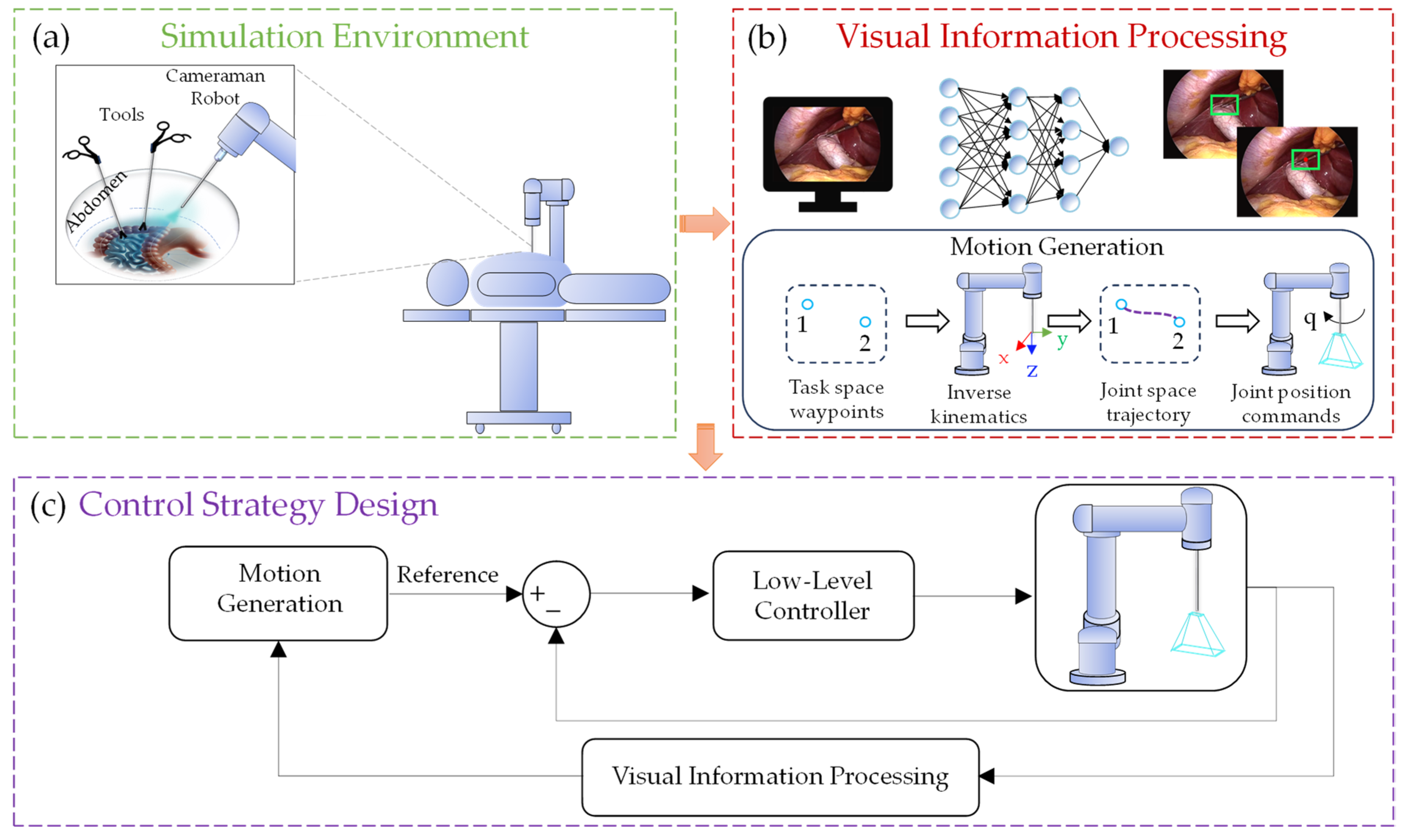
Methodology of the Neuro-Visual Adaptive Controller (NVAC) Operation. (a) Simulation Environment: This represents the virtual scenario where the camera-holding robot interacts with surgical tools and the patient. (b) Visual Information Processing: In this stage, visual data are interpreted, and motion trajectories for the robot are generated using computer vision models and inverse kinematics. (c) Control Strategy Design: The robot’s response is defined based on the processed visual information, adjusting its movement through the low-level MRAC-PD-CfC-mmRNN controller.
Figure 1.
Methodology of the Neuro-Visual Adaptive Controller (NVAC) Operation. (a) Simulation Environment: This represents the virtual scenario where the camera-holding robot interacts with surgical tools and the patient. (b) Visual Information Processing: In this stage, visual data are interpreted, and motion trajectories for the robot are generated using computer vision models and inverse kinematics. (c) Control Strategy Design: The robot’s response is defined based on the processed visual information, adjusting its movement through the low-level MRAC-PD-CfC-mmRNN controller.
Figure 2.
Simulation environment in CoppeliaSim representing a surgical scenario with a human mannequin. A laparoscope equipped with assisted vision is depicted operating within the simulated environment.
Figure 2.
Simulation environment in CoppeliaSim representing a surgical scenario with a human mannequin. A laparoscope equipped with assisted vision is depicted operating within the simulated environment.
Figure 3.
Examples of the dataset used in the study. (a) Images from the original CholecSeg8k dataset; (b) images captured in MatLab® from the CoppeliaSim environment; (c) example of annotations in a subset of images from the original dataset, labeling only the tip of the surgical tool as ground truth.
Figure 4.
Representation of the structure and joint configuration of the UR5 robot using the Denavit-Hartenberg convention.
Figure 4.
Representation of the structure and joint configuration of the UR5 robot using the Denavit-Hartenberg convention.
Figure 5.
YOLO11 architecture. The diagram illustrates the main components of the model: convolutional layers (Conv) combined with C2PSA blocks at the top, processing pathways featuring BottleNeck and SPPF on the left, and specialized modules such as PSA, FFN, and Detect blocks.
Figure 5.
YOLO11 architecture. The diagram illustrates the main components of the model: convolutional layers (Conv) combined with C2PSA blocks at the top, processing pathways featuring BottleNeck and SPPF on the left, and specialized modules such as PSA, FFN, and Detect blocks.
Figure 6.
CfC-mmRNN neural network architecture. The figure illustrates the combination of Closed-Form Continuous-Time (CfC) networks with LSTM, forming the CfC-mmRNN architecture. On the left, a traditional LSTM cell is depicted, while on the right, the CfC cell is shown, incorporating a time vector and neural network heads (g, f, h). This integration enhances computational efficiency and the modeling of temporal dynamics.
Figure 7.
Schematic of the MRAC-PD-CfC-mmRNN low-level controller. The MRAC-PD-CfC-mmRNN controller is responsible for managing the dynamic response of the robotic manipulator within the NVAC framework. The controller accounts for the robot’s dynamics and incorporates a reference model that adjusts the desired trajectory using adaptive gains (, ). The CfC-mmRNN network predicts the inverse torque (), supplemented by proportional, derivative, and adaptive terms to enhance control stability and robustness.
Figure 8.
Workspace of the camera-holding robot. (a) Representation of the robot’s complete workspace, including the laparoscope (blue points), with a restricted operational region in the abdominal area (red lines); (b) example of a trajectory within the restricted workspace, showing the starting point (SP, green circle), endpoint (EP, red star), and planned trajectory (blue line). Top and front views enable analysis of the trajectory relative to imposed limits, highlighting compliance with spatial constraints.
Figure 9.
Example of trajectories generated within the restricted workspace for training the robot’s inverse model.
Figure 9.
Example of trajectories generated within the restricted workspace for training the robot’s inverse model.
Figure 10.
Performance curves of YOLO11 training across training epochs. The top row displays the training losses for box detection (train/box_loss), classification (train/cls_loss), and distribution focal loss (train/dfl_loss), along with precision and recall metrics. The bottom row presents the validation losses (val/box_loss, val/cls_loss, val/dfl_loss) and the mAP50 and mAP50–95 metrics. These plots demonstrate the model’s effective convergence during training and its ability to generalize on validation data.
Figure 11.
Detection of the surgical tool tip. (a) Detection results on the test set using YOLO11n; (b) localization of the centroid of the bounding boxes.
Figure 11.
Detection of the surgical tool tip. (a) Detection results on the test set using YOLO11n; (b) localization of the centroid of the bounding boxes.
Figure 12.
Validation of the inverse model training for a test trajectory. The torques estimated by the inverse model (solid line) are compared with the actual torques applied by the robot (dashed line) across each of the six joints, verifying the model’s accuracy in reproducing the system’s dynamics.
Figure 13.
Trajectory tracking performance of the implemented controllers. (a) Desired Cartesian trajectory 1 for Scenario 1. (b) Desired Cartesian trajectory 2 for Scenario 2.
Figure 13.
Trajectory tracking performance of the implemented controllers. (a) Desired Cartesian trajectory 1 for Scenario 1. (b) Desired Cartesian trajectory 2 for Scenario 2.
Figure 14.
Simulation results for the implemented control strategies. (a) Tracking of the desired Cartesian trajectory 1 on the x-axis; (b) tracking of the desired Cartesian trajectory 2 on the x-axis.
Figure 14.
Simulation results for the implemented control strategies. (a) Tracking of the desired Cartesian trajectory 1 on the x-axis; (b) tracking of the desired Cartesian trajectory 2 on the x-axis.
Figure 15.
Simulation results for the implemented control strategies. (a) Tracking of the desired Cartesian trajectory 1 on the y-axis; (b) tracking of the desired Cartesian trajectory 2 on the y-axis.
Figure 15.
Simulation results for the implemented control strategies. (a) Tracking of the desired Cartesian trajectory 1 on the y-axis; (b) tracking of the desired Cartesian trajectory 2 on the y-axis.
Figure 16.
Simulation results for the implemented control strategies. (a) Tracking of the desired Cartesian trajectory 1 on the z-axis; (b) tracking of the desired Cartesian trajectory 2 on the z-axis.
Figure 16.
Simulation results for the implemented control strategies. (a) Tracking of the desired Cartesian trajectory 1 on the z-axis; (b) tracking of the desired Cartesian trajectory 2 on the z-axis.
Figure 17.
Cartesian trajectory tracking under external disturbances. (a) Trajectory 1, Scenario 3; (b) trajectory 2, Scenario 4.
Figure 17.
Cartesian trajectory tracking under external disturbances. (a) Trajectory 1, Scenario 3; (b) trajectory 2, Scenario 4.
Figure 18.
Cartesian tracking errors in surgical instrument tracking for Scenario 3. The figure compares the tracking errors of the designed controllers along the Cartesian axes (x, y, z).
Figure 18.
Cartesian tracking errors in surgical instrument tracking for Scenario 3. The figure compares the tracking errors of the designed controllers along the Cartesian axes (x, y, z).
Figure 19.
Cartesian tracking errors in surgical instrument tracking for Scenario 4. The figure compares the tracking errors of the designed controllers along the Cartesian axes (x, y, z).
Figure 19.
Cartesian tracking errors in surgical instrument tracking for Scenario 4. The figure compares the tracking errors of the designed controllers along the Cartesian axes (x, y, z).
Figure 20.
Examples of surgical tool detection with YOLO11n in challenging scenarios, including low lighting, partial occlusion, smoke presence, and small instrument detection.
Figure 20.
Examples of surgical tool detection with YOLO11n in challenging scenarios, including low lighting, partial occlusion, smoke presence, and small instrument detection.
Table 1.
Design parameters for the NVAC control strategy.
Table 1.
Design parameters for the NVAC control strategy.
| Parameters | Joint 1 | Joint 2 | Joint 3 | Joint 4 | Joint 5 | Joint 6 |
|---|
| 100 | 3000 | 320 | 80 | 30 | 2 |
| 100 | 380 | 80 | 20 | 8 | 2 |
| 4 | 4 | 4 | 4 | 3 | 3 |
| 3 | 3 | 2 | 2 | 3 | 3 |
Table 2.
Neural network training parameters for system identification and tool tip detection.
Table 2.
Neural network training parameters for system identification and tool tip detection.
| Parameters | CfC-mmRNN | Parameters | YOLO11n |
|---|
| Epochs | 50 | Epochs | 300 |
| Initial Learning Rate | 0.001 | Initial Learning Rate | 0.01 |
| Batch Size | 64 | Batch Size | 16 |
| Activation Function | GELU | Optimizer | SGDM |
| Optimizer | Adam | Momentum | 0.937 |
| Weight Decay | | Weight Decay | |
Table 3.
Computational cost of trained neural network models.
Table 3.
Computational cost of trained neural network models.
| Model | Parameters | Memory | Inference Speed |
|---|
| YOLO11x | 56,874,931 | 111.7 MB | 34.8 ms |
| YOLO11n | 2,590,035 | 5.37 MB | 9.5 ms |
| CfC-mmRNN | 197,638 | 798 KB | 26 ms |
Table 4.
Performance indexes for Cartesian and joint positions under trajectory 1.
Table 4.
Performance indexes for Cartesian and joint positions under trajectory 1.
| PIs | Controller | x | y | z | Joint 1 | Joint 2 | Joint 3 | Joint 4 | Joint 5 | Joint 6 |
|---|
| MAE | PID | 0.0047 | 10−5 | 0.0081 | 10−5 | 0.0065 | 0.0120 | 0.0031 | 0.0008 | 0.0005 |
| SMC | 0.0045 | 0.0002 | 0.0031 | 10−5 | 0.0020 | 0.0098 | 0.0027 | 0.0001 | 0.0002 |
| MRAC-PD | 10−5 | 10−6 |
10−5 | 10−5 | 10−5 | 10−5 | 10−5 | 10−5 | 0.0002 |
| Proposed | 10−6 | 10−6 | 10−5 | 10−5 | 10−5 | 10−5 | 10−5 | 10−5 | 0.0001 |
| ITAE | PID | 0.5538 | 0.0084 | 0.9556 | 0.0066 | 0.7814 | 1.4354 | 0.3425 | 0.0709 | 0.0363 |
| SMC | 0.5383 | 0.0174 | 0.3751 | 0.0028 | 0.2325 | 1.1793 | 0.3337 | 0.0289 | 0.0116 |
| MRAC-PD | 0.0003 | 0.0002 | 0.0008 | 0.0015 | 0.0014 | 0.0013 | 0.0008 | 0.0023 | 0.0105 |
| Proposed | 0.0003 | 0.0004 | 0.0012 | 0.0013 | 0.0021 | 0.0010 | 0.0008 | 0.0022 | 0.0105 |
| ITSE | PID | 0.0026 | 10−6 | 0.0077 | 10−7 | 0.0052 | 0.0174 | 0.0010 | 10−5 | 10−5 |
| SMC | 0.0024 | 10−6 | 0.0011 | 10−7 | 0.0004 | 0.0117 | 0.0009 | 10−6 | 10−6 |
| MRAC-PD | 10−8 | 10−10 | 10−8 | 10−8 | 10−7 | 10−7 | 10−8 | 10−8 | 10−6 |
| Proposed | 10−9 | 10−9 | 10−8 | 10−8 | 10−8 | 10−8 | 10−8 | 10−8 | 10−6 |
Table 5.
Performance indexes for Cartesian and joint positions under trajectory 2.
Table 5.
Performance indexes for Cartesian and joint positions under trajectory 2.
| PIs | Controller | x | y | z | Joint 1 | Joint 2 | Joint 3 | Joint 4 | Joint 5 | Joint 6 |
|---|
| MAE | PID | 0.0049 | 10−4 | 0.0084 | 10−4 | 0.0055 | 0.0121 | 0.0031 | 0.0013 | 0.0024 |
| SMC | 0.0045 | 10−4 | 0.0033 | 10−5 | 0.0029 | 0.0098 | 0.0027 | 10−4 | 0.0011 |
| MRAC-PD | 10−5 | 10−6 | 10−5 | 10−5 | 10−5 | 10−5 | 10−5 | 10−5 | 0.0015 |
| Proposed | 10−6 | 10−6 | 10−5 | 10−5 | 10−5 | 10−5 | 10−5 | 10−5 | 0.0013 |
| ITAE | PID | 0.9228 | 0.0373 | 1.6236 | 0.0174 | 1.0312 | 2.3259 | 0.5386 | 0.3276 | 0.5482 |
| SMC | 0.8693 | 0.0582 | 0.6403 | 0.0046 | 0.5909 | 1.8829 | 0.5075 | 0.0440 | 0.2332 |
| MRAC-PD | 0.0012 | 10−4 | 0.0052 | 0.0022 | 0.0078 | 0.0054 | 0.0073 | 0.0034 | 0.3128 |
| Proposed | 0.0013 | 10−4 | 0.0048 | 0.0022 | 0.0067 | 0.0051 | 0.0078 | 0.0033 | 0.3126 |
| ITSE | PID | 0.0044 | 10−6 | 0.0138 | 10−6 | 0.0056 | 0.0282 | 0.0015 | 10−3 | 0.0073 |
| SMC | 0.0039 | 10−5 | 0.0021 | 10−7 | 0.0019 | 0.0185 | 0.0013 | 10−5 | 0.0035 |
| MRAC-PD | 10−8 | 10−9 | 10−7 | 10−8 | 10−7 | 10−7 | 10−7 | 10−7 | 0.0060 |
| Proposed | 10−8 | 10−9 | 10−7 | 10−8 | 10−7 | 10−7 | 10−7 | 10−7 | 0.0055 |
Table 6.
Performance indexes for Cartesian and joint positions under Scenario 3.
Table 6.
Performance indexes for Cartesian and joint positions under Scenario 3.
| PIs | Controller | x | y | z | Joint 1 | Joint 2 | Joint 3 | Joint 4 | Joint 5 | Joint 6 |
|---|
| MAE | PID | 10−5 | 0.0065 | 0.0121 | 10−5 | 0.0065 | 0.0121 | 0.0033 | 0.0007 | 0.0004 |
| SMC | 0.0046 | 0.0002 | 0.0032 | 10−5 | 0.0019 | 0.0100 | 0.0029 | 0.0001 | 0.0002 |
| MRAC-PD | 10−5 | 10−6 | 10−5 | 10−5 | 10−5 | 0.0001 | 10−5 | 10−5 | 0.0002 |
| Proposed | 10−5 | 10−6 | 10−5 | 10−5 | 10−5 | 10−5 | 10−5 | 10−5 | 0.0001 |
| ITAE | PID | 0.0066 | 0.7860 | 1.4465 | 0.0066 | 0.7860 | 1.4465 | 0.3767 | 0.0708 | 0.0362 |
| SMC | 0.5538 | 0.0177 | 0.3841 | 0.0028 | 0.2285 | 1.1966 | 0.3613 | 0.0289 | 0.0116 |
| MRAC-PD | 0.0046 | 0.0004 | 0.0053 | 0.0014 | 0.0049 | 0.0080 | 0.0077 | 0.0022 | 0.0105 |
| Proposed | 0.0046 | 0.0003 | 0.0057 | 0.0013 | 0.0057 | 0.0078 | 0.0076 | 0.0023 | 0.0105 |
| ITSE | PID | 10−7 | 0.0052 | 0.0176 | 10−7 | 0.0052 | 0.0176 | 0.0016 | 10−5 | 10−5 |
| SMC | 0.0026 | 10−6 | 0.0012 | 10−7 | 0.0004 | 0.0121 | 0.0013 | 10−6 | 10−5 |
| MRAC-PD | 10−6 | 10−9 | 10−6 | 10−8 | 10−6 | 10−6 | 10−6 | 10−8 | 10−6 |
| Proposed | 10−6 | 10−9 | 10−6 | 10−8 | 10−6 | 10−6 | 10−6 | 10−8 | 10−6 |
Table 7.
Performance indexes for Cartesian and joint positions under Scenario 4.
Table 7.
Performance indexes for Cartesian and joint positions under Scenario 4.
| PIs | Controller | x | y | z | Joint 1 | Joint 2 | Joint 3 | Joint 4 | Joint 5 | Joint 6 |
|---|
| MAE | PID | 0.0049 | 10−4 | 0.0084 | 10−4 | 0.0055 | 0.0121 | 0.0032 | 0.0013 | 0.0024 |
| SMC | 0.0046 | 10−4 | 0.0033 | 10−5 | 0.0029 | 0.0099 | 0.0028 | 10−4 | 0.0011 |
| MRAC-PD | 10−5 | 10−6 | 10−5 | 10−5 | 10−5 | 10−5 | 10−5 | 10−5 | 0.0015 |
| Proposed | 10−5 | 10−6 | 10−5 | 10−5 | 10−5 | 10−5 | 10−5 | 10−5 | 0.0013 |
| ITAE | PID | 0.9378 | 0.0376 | 1.6297 | 0.0173 | 1.0364 | 2.3382 | 0.5698 | 0.3276 | 0.5482 |
| SMC | 0.8863 | 0.0597 | 0.6504 | 0.0046 | 0.5864 | 1.9021 | 0.5380 | 0.0440 | 0.2331 |
| MRAC-PD | 0.0060 | 10−4 | 0.0086 | 0.0022 | 0.0097 | 0.0119 | 0.0141 | 0.0033 | 0.3128 |
| Proposed | 0.0059 | 0.0012 | 0.0083 | 0.0022 | 0.0088 | 0.0115 | 0.0145 | 0.0032 | 0.3126 |
| ITSE | PID | 0.0046 | 10−6 | 0.0138 | 10−6 | 0.0056 | 0.0285 | 0.0022 | 10−4 | 0.0073 |
| SMC | 0.0041 | 10−5 | 0.0022 | 10−7 | 0.0018 | 0.0190 | 0.0017 | 10−5 | 0.0034 |
| MRAC-PD | 10−6 | 10−8 | 10−6 | 10−8 | 10−6 | 10−5 | 10−5 | 10−7 | 0.0060 |
| Proposed | 10−6 | 10−8 | 10−6 | 10−8 | 10−6 | 10−5 | 10−5 | 10−7 | 0.0055 |


