High-Voltage Overhead Power Line Fault Location Through Sequential Determination of Faulted Section

Abstract

Overhead power lines (OHPLs) represent the backbone of electric power systems and connect generation sources with consumers. The power supply reliability and maintenance costs of power grids largely depend on accurate fault location on OHPLs, as this significantly affects the speed of power supply restoration and reduces equipment downtime. This article proposes a new approach to fault location which includes the division of the OHPL bypass (inspection) zone into sections with subsequent implementation of a faulted section location procedure. This article substantiates the application of sequential multi-hypothesis analysis, which allows us to adapt the decision-making process regarding the OHPL faulted section to the peculiarities of emergency event oscillogram distortion and the conditions for estimating their parameters. According to the results of our calculations, it is noted that the application of sequential analysis practically does not affect the speed of OHPL fault location but does ensure unambiguity in decision making regarding the faulted section under the influence of random factors.

1. Introduction

Overhead power lines (OHPLs) form the backbone of electric power systems, connecting generation sources with consumers. The reliability of their power supply and the maintenance costs of power grids are largely dependent on accurate fault location (FL) on OHPLs, as it significantly affects the speed of power supply restoration and reduces equipment downtime [1,2,3].

It should be noted that a large part of OHPL outages are transient, meaning that the OHPL remains in operation after a successful automatic reclosure. These transient faults can be self-clearing or, under certain conditions, can develop into permanent faults. On OHPLs, unstable faults can be caused by the following: the throwing of various objects on wires, power overlapping in suspension insulator garlands, the convergence of phase wires under windy conditions or “wire dancing”, and others. In this case the procedure of fault searching during the post-accident bypass of OHPLs becomes much more complicated, and the importance of developing accurate and reliable methods and devices for FL increases [4,5,6,7,8,9,10,11,12].

The development of FL devices can be performed using various physical principles and algorithms. The relative error of traveling wave methods in FL [13,14,15,16,17], including those based on the active probing of OHPLs [17], is significantly lower than the error of traditional FL devices based on emergency mode parameters (EMPs) [18,19,20,21,22]. However, the high cost of wave-based FL devices still limits the possibility of their mass application.

Table 1. The main categories of existing methods for determining FL.

Method Category	Main Types of Methods	Advantages	Limitations
Traditional (manual)	Visual overflight (helicopter, drone, etc.). Walk-through with teams. Eyewitness testimony.	- Direct confirmation of fault and its nature. - Does not require complex mathematical apparatus.	- Extremely slow and labor-intensive. - Dependent on weather, time of day, and terrain. - High cost and risk to personnel.
Traditional, analytical (distance)	Pulse (reflectometers). Based on the analysis of transient processes or emergency mode parameters (EMPs). Impedance methods.	- High speed of result delivery. - No line shutdown required. - EMP methods are quite accurate and reliable in most cases.	- Accuracy decreases with high-resistance faults. - Dependence on line parameters and transition resistance, and low power quality indicators (PQIs).
Modern, intelligent (passive or active)	Methods based on wave processes (traveling wave). Methods based on artificial intelligence (AI) and machine learning (ML).	- Very high accuracy. - Fast response. - Low dependence on contact resistance and network conditions.	- Requires expensive equipment (ADC, GPS, etc.). - Data processing is complex. - Efficiency decreases for near-faults.
Statistical (probabilistic)	Analysis of fault frequency by section, taking into account “weak points” (thunderstorm activity, ice, wind, insulation condition, diagnostic data, etc.). Bayesian networks/fuzzy logic: combination of multiple factors (current, voltage, weather, geodata, etc.) to assess the most probable section.	- Enables identification of the most vulnerable sections of transmission lines for proactive measures. - Increases reliability by combining data from other methods with historical, operational, and modeled data. - Enables generation of multiple probable points with reliability assessments.	- Does not pinpoint the exact location of fault, only a probabilistic zone. - Requires a huge array of historical, operational, or simulated data. - Complexity of model setup and verification.
Using simulation modeling	Creation of a “digital twin” of the power transmission line: a detailed model in a software suite, simulation of 1000+ fault and short-circuit scenarios (various locations, types, and resistances). Comparative analysis: comparison of actual fault waveforms with a database of simulated references, using machine learning methods for classification.	- Deep verification: the ability to test and refine FL algorithms in complex scenarios (cascading accidents, short circuits, etc.). - AI training: creation of extensive datasets for training neural networks when real data are insufficient. - Proactive analysis: assessment of the vulnerability and accuracy of FL for a line that has not yet been built or upgraded. - Reliability enhancement: allows you to select the best FL algorithm for a specific network.	- High computational costs for creating an accurate model and running multiple simulations. - Requires highly accurate line and network parameters for model validity. - Indirect method: not used for real-time fault location but rather as a preparation, configuration, and analysis tool.
Faulted area determination (segmental)	The “emergency indicator” method: installing sensors with indicators. The current derivative (dI/dt) analysis method: recording the moment and magnitude of a sudden current change. Distributed monitoring (phase-sensitive systems): comparing the direction of power or current phasors at different points along the line to isolate a section.	- Simplicity and clarity: clearly indicates the area between two supports or sensors. - High reliability and noise immunity (for modern data transmission systems). - No complex substation calculations required. - Effective in extensive networks.	- Low accuracy: identifies the faulted section rather than the point (hundreds of meters/kilometers long). - Requires installation and maintenance of multiple devices along the entire line. - Costs for communication infrastructure and sensor power supply.

provides an overview of the main categories of existing FL methods with their main advantages and limitations, which is based on an analysis of sources [3,4,5,6,7,8,9,10,11,12,13,14,15,16,17,18,19,20,21,22].

When implementing an FL system, it is crucial not only to accurately estimate the fault point on the OHPL but also to establish an appropriate inspection zone for the line crew(s) [1,2,9]. This zone must satisfy two conflicting requirements. On the one hand, it must be sufficiently large to ensure that the actual fault location falls within its boundaries, accounting for the influence of random factors. On the other hand, it should be as small as possible to minimize the time and economic costs associated with inspecting the line. Consequently, defining this zone requires careful consideration of the OHPL design specifics and the full range of random factors that affect FL accuracy.

According to Russian regulatory documents, the following requirements have been established for determining the OHPL inspection zone. Following an emergency shutdown, the maximum extent of this zone must be calculated based on the readings from the FL devices:

• ±15% of the OHPL length for lines up to and including 50 km;
• ±10% for OHPLs over 50 km up to and including 100 km;
• ±7% for OHPLs from 100 to 300 km inclusive;
• ±5% for OHPLs with a length of 300 km or more.

However, when determining the OHPL bypass zone, refs. [8,10] do not take into account the FL errors, those associated with power quality indicator (PQI) deviations. Such deviations can be caused by the presence of harmonic components caused by transients during short circuits on OHPLs in the current and voltage emergency oscillograms, the non-stationarity of industrial load power consumption influence, the use of power electronics elements, the presence of renewable energy sources with stochastic nature of power generation, etc.

Let us formulate the FL location problem as a classification task which involves determining whether a fault belongs to one of the segments within the OHPL inspection zone. Due to the influence of the random factors mentioned above, the decision-making process in FL determination is stochastic. It involves processing current and voltage emergency oscillograms recorded over a limited time interval.

Furthermore, the following considerations contribute to the multi-stage nature of decision making in OHPL fault location [15,20,23]:

• Using complete parameter arrays. It is advantageous to use full sets of current and voltage parameters from the entire emergency event recording, rather than basing the fault location decision on a single time slice of an oscillogram.
• Adaptive parameter selection. The approach allows decisions to be made using either a reduced set of parameters when signal distortions are minimal or an extended set for severe (“deep”) distortions. This ensures accurate faulted section identification with the required reliability indicators while optimizing computational time and resources.
• Data source integration. The methodology supports the use of emergency oscillograms (or fault location results) from various devices—such as dedicated FL units, fault recorders, protection relays, automation terminals, energy management systems, and synchrophasors—located on adjacent OHPL sections that recorded the event.

This paper analyzes established methods for identifying the faulted section in an OHPL and investigates the application of multi-hypothesis sequential analysis to this problem, using Reed’s algorithm as a case study.

2. Analysis of Known Methods for Locating a Transmission Line Faulted Section

Two methods applied in electric power grids and railway contact networks are considered [24,25]. The first method [24] is an interval-based approach designed to reduce the span of the line segment that contains the fault. The second method [25] involves dividing the transmission line into discrete sections to solve the problem of pinpointing the exact faulty section.

2.1. Method of Interval Determination of Transmission Line Faulted Section

It is assumed that the method and the FL device [24] do not use any measurements in the conventional sense: neither resistance measurements, nor fault resistivity criteria, nor transmission models, etc. [1]. Instead, a new approach is introduced, in which the sought-after fault mode is considered to be each mode simulated by the simulation model for which the same vector of measured parameters (currents and/or voltages from one or two or more ends of the OHPL) is observed, as is observed from the protected object.

An arbitrary discrepancy criterion, such as the total relative error, is proposed as a criterion for determining the proximity of the vector of measured values of the simulated mode to the vector of measured values from the facility (OHPL). This is believed to provide an additional opportunity to estimate not only the distance from the FL but also other parameters of the power transmission system and the FL: the magnitude of contact resistance at the fault location, the transmission angle, the resistance of the power supply systems, etc.

Let us assume that there is OHPL 1, which connects feeding substations 2 and 3 (Figure 1). In the case of one-sided observation, only the current vector and/or the voltage vector on side 4 are used, while in the case of two-sided observation, the vectors on side 5 are additionally used. The following notations are introduced in Figure 1: i and u—electric current and voltage vectors of the multiconductor system; k—discrete time; s and r—indices of substations 2 and 3.

It is required to determine the OHPL section that is guaranteed to include point 6, and the section should have the minimum possible length.

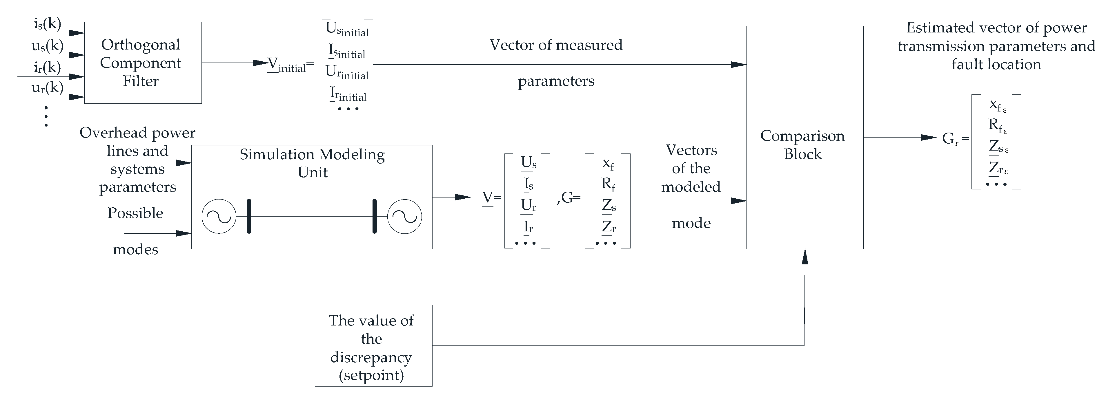
The counts of the observed values (i_s(k), u_s(k), i_r(k), u_r(k), …) are processed in the orthogonal component filter (Figure 2) and form complex values of the vector of the measured parameters V_initial, which represents the first input to the comparison block.

The simulation block (Figure 2) calculates a variety of fault modes for the protected object (OHPL), as well as modes preceding the fault.

Parameters for simulation modeling refer to the a priori information about the transmission line. The simulation block generates current and/or voltage magnitude vectors (denoted by V) and object parameter vector (denoted by G) of the modeled modes to which these currents and/or voltages correspond. The data are transferred to the comparison block as the second input.

The total error ε magnitude (or other discrepancy criterion) is set by the setpoint for the comparison block, at the output of which the required object parameter vector of only those fault modes for which the conditions of vector proximity are met is formed (denoted by G_ε).

Faulted section coordinate value set x_f (x_f ∈ X_fε, X_fε ∈ G_ε) of the selected modes constitutes the sought interval, guaranteed to contain the real faulted location coordinate. Similarly, it is possible to estimate the interval containing the sought value of any other object parameter, for example, the transient resistance value R_f (R_f ∈ R_fε, R_fε ∈ G_ε).

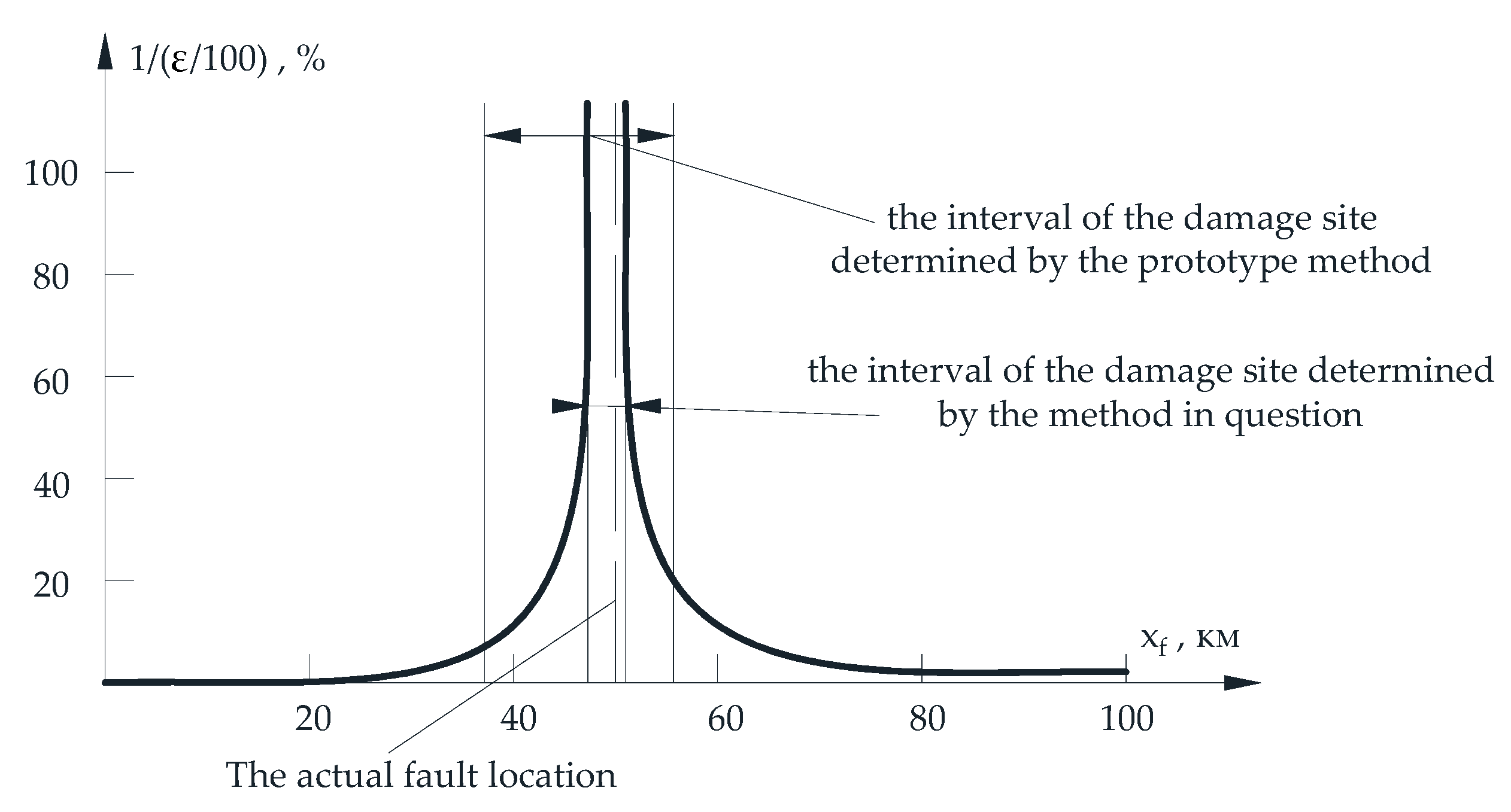
Figure 3 shows the comparison results of the methods presented in refs. [24,26] with the same information base and under equal conditions. From the Figure 3 analysis, it can be seen that the area determined by the method in ref. [26] is [37.181; 55.708] km or 18.527% of the line length. The interval of the distance from the fault for the method considered in ref. [24] is [47.30; 50.96] km or 3.66% of the line length. Thus, the method in ref. [24] allows us to obtain a much smaller section of the OHPL, including the true faulted location coordinate, and consequently, to achieve greater accuracy.

2.2. Method of Locating a Faulted Section in a Contact Traction Electrical Network

The AC railroad traction network is a complex heterogeneous electrical circuit which has a number of traction current conductors: contact network conductors, feed, shielding, suction lines and rails, and sleepers [27]. The contact network and rails, together with the ground, form interconnected electromagnetic circuits. On multi-track sections the electromagnetic connections of both track network elements turn out to be quite complicated.

The numerical values of the parameters that constitute the short-circuit loop resistance in the contact network have a random component. This is because they depend on numerous factors, such as the nature of the electric arc, the power supply scheme, the mutual influence of adjacent paths, the distance from the fault, and the voltage levels on the busbars of adjacent substations. Furthermore, when developing a method for determining the fault location, none of the short-circuit loop parameters can be used as the sole criterion.

To determine the short circuit location, the pattern recognition methodology is used, in which the measured set (vector) of parameters x_measured is compared with the set of calculated parameters x obtained from the simulation modeling (calculation) results [25].

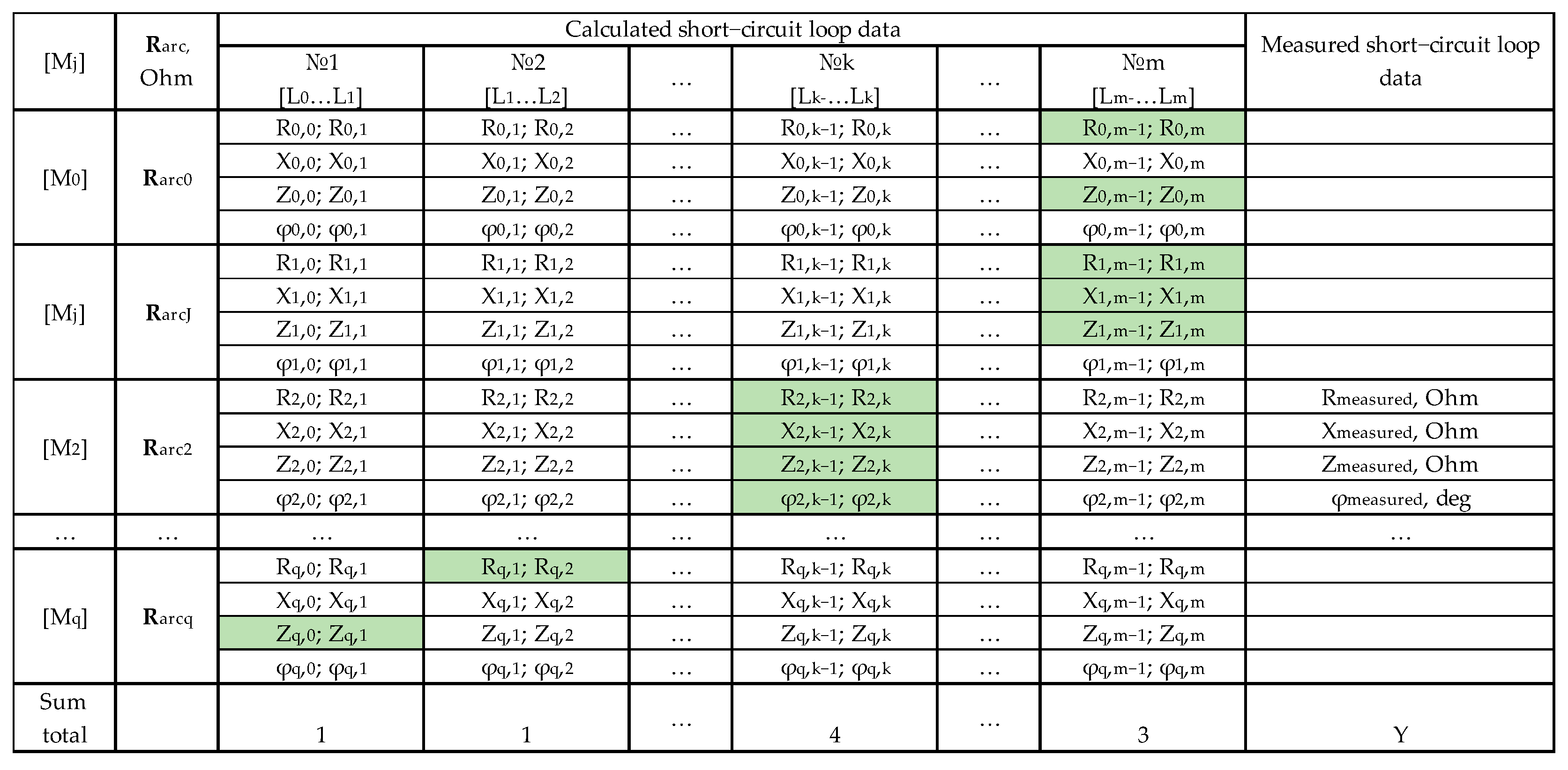
Parameter vectors x are summarized in matrices M_j (where j characterizes the fault resistance) and are calculated at the interval boundaries ΔL_k = L_k − L_k−1, into which the traction network is conventionally divided (Figure 4). Elements x_measured and x are considered to coincide if x_k > x_measured > x_k−1.

The number of matches when comparing the calculated elements x with the measured x_measured is summarized in the columns of aggregate matrix M (highlighted in color in Figure 5) and recorded in the bottom row of matrix M. The column of matrix M that has the highest number of matches indicates the short circuit location. Matrix M includes the calculated derived parameters of the short-circuit loops: R—active; X—inductive; and Z—impedance. It also includes the values of phase angles φ and arc resistances R_arc.

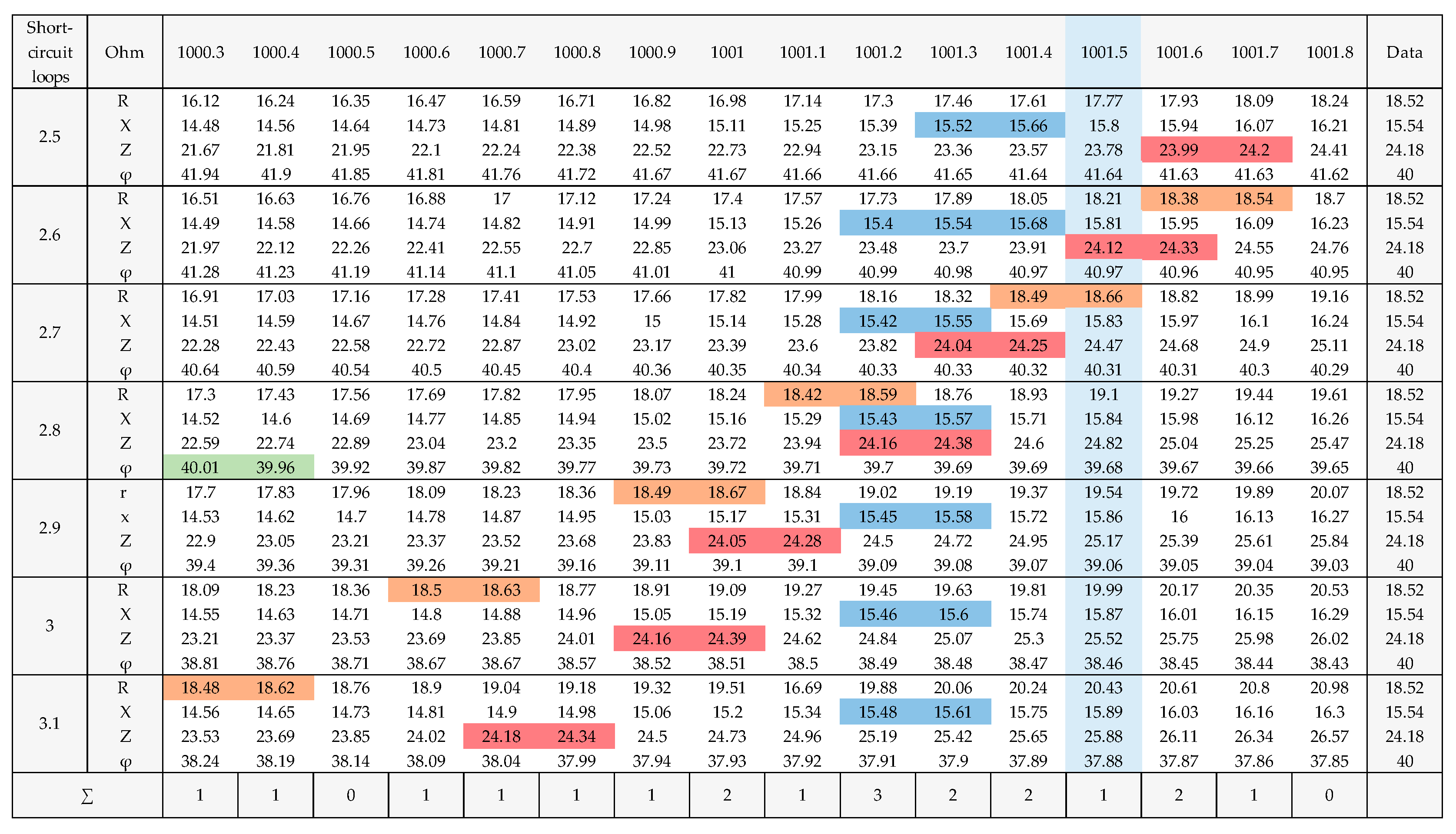
Figure 5 shows an example of matrix M from model experiments [25]. The upper row of the matrix contains the track segments coordinates with step ΔL = 0.1 km, into which the traction network is divided. The leftmost column of the matrix contains the column vector R_arc, which contains the possible arc parameters with a step of 0.1 ohms. In Figure 6, the matches of the specified parameters of short circuit loops (R, X, Z, φ) are highlighted in different colors.

The analysis of Figure 6 shows that the greatest coincidence of the calculated and measured short-circuit loop parameters corresponds to the arc of 2.8 Ohm with a short-circuit location at 1001.2 km. Taking into account that the short-circuit was modeled at a distance of 1001.5 km, the difference between the calculated and real faulted locations was 200–300 m.

3. Consistent Criterion for Selecting a Hypothesis About a Faulted Section from a Set of Overhead Transmission Line Sections Within Its Bypass Area

It is assumed that k experiments with sampled data at each step of the procedure are conducted to perform sequential analysis for selecting the faulted section within the OHPL bypass zone.

Based on the each of the experimental results, one of (M + 1) decisions is made:

• To end the experiment by accepting hypothesis H₁ (site number 1 is faulted);
• To end the experiment by accepting hypothesis H₂ (site number 2 is faulted);
• To finish the experiment by accepting hypothesis H_M (site number M is faulted);
• …;
• To continue the experiment by making additional observations.

Thus, the procedure is performed sequentially: based on the first observation, one of (M + 1) decisions is made, and when one of the first M decisions is selected, the process ends. If the decision number (M + 1) is selected, the next (second) observation is made. Now one of the (M + 1) decisions is made based on the first two sample values. If the choice is the last (M + 1) decision, a third experiment is performed. The process continues until one of the first M solutions is selected. The number of hypotheses corresponds to the number of OHPL length partitions, which are selected based on operational requirements. Ideally, the section length corresponds to the span length (the distance between transmission line supports).

In the general case, the decision concerning the faulted section is made on the basis of the current and voltage parameter x vector, characteristic and corresponding to the faulted section with the number m (m = 1, …, M). In this case, the current and voltage parameter vector x = {x₁, x₂, …} is generally random, because it can include distorting components, for example, associated with electric power quality indicator (PQI) deviations from the normative values [28].

Since hypotheses H₁, …, H_m, …, H_M mutually exclude each other and exhaust all possible cases for the selected vector x values, then one (and only one) of hypotheses H₁, …, H_M is consistent with a particular set of vector x values.

It should be added that it is possible to numerically express the significance of economic losses due to various wrong decisions. Let us introduce the functions w₁(x), …, w_m(x), …, w_M(x), where w_m(x) is a non-negative function defining the additional economic costs associated with the extended OHPL bypass and resulting from hypothesis H_m, when the current and voltage parameter x vector is true. Obviously, w_m(x) = 0 for all points x included in section m, since for such points, the correct decision regarding the OHPL faulted location will be made.

Note that the functions w₁(x), …, w_m(x), …, w_M(x) correspond to the FL errors weight functions, since the numerical ratio w₁(x), …, w_m(x), …, w_M(x), i.e., the ratio of fault location error prices, should determine the decision rule concerning the faulted OHPL section.

Risk R(x) for the current and voltage parametric point x we will call the mathematical loss expectation caused by incorrect decisions with respect to the faulted section, when the x concrete value is true.

Let the probability of accepting hypothesis H_m equal P_m(x) and the loss function associated with this decision equal w_m(x); then the risk (mathematical loss expectation) is equal to

$$\mathrm{R}(\mathrm{x})={\mathrm{P}}_1(\mathrm{x})\cdot {\mathrm{w}}_1(\mathrm{x})+\dots +{\mathrm{P}}_{\mathrm{m}}(\mathrm{x})\cdot {\mathrm{w}}_{\mathrm{m}}(\mathrm{x})+\dots +{\mathrm{P}}_{\mathrm{M}}(\mathrm{x})\cdot {\mathrm{w}}_{\mathrm{M}}(\mathrm{x})={\displaystyle {\sum }_{\mathrm{m}=1}^{\mathrm{M}}{\mathrm{P}}_{\mathrm{m}}(\mathrm{x})\cdot {\mathrm{w}}_{\mathrm{m}}(\mathrm{x}).}$$

(1)

We will assume that the optimal decision rule regarding OHPL faulted section m will minimize risk R(x) in case of making wrong decisions.

The selection and obtaining of functional dependencies w₁(x), …, w_M(x) from the practical point of view may present certain difficulties, and their application may lead to complex calculation algorithms. Therefore, it is reasonable to use rough approximations of such dependencies or simplifications. The most widely used approximation is the use of a “semi-simple cost function” [29] corresponding to the following expression:

$${\mathrm{w}}_{\mathrm{m}}(\mathrm{x})=\left\{\begin{array}{c}0, \mathrm{if}\cos \mathrm{t}\mathrm{function}\mathrm{is}\mathrm{less}\mathrm{o}\mathrm{r}\mathrm{equals}\mathrm{than}{\mathrm{c}}_{\mathrm{m}}\mathrm{v}\mathrm{a}\mathrm{l}\mathrm{u}\mathrm{e},\hfill \\ \mathrm{c}, \mathrm{if}\cos \mathrm{t}\mathrm{function}\mathrm{i}\mathrm{s}\mathrm{bigger}\mathrm{than}{\mathrm{c}}_{\mathrm{m}}\mathrm{v}\mathrm{a}\mathrm{l}\mathrm{u}\mathrm{e},\hfill \end{array}\right.$$

(2)

where c is a chosen positive constant, which, depending on w_m(x), can take only two values: 0 or 1. In some cases [29], c = 1 is taken since multiplying the risk function by a constant multiplier does not affect decision rule realization. Further we will consider only semi-simple cost functions, since even the application of such functions allows for the implementation of higher-accuracy FL algorithms.

In sequential analysis procedures with simplified weight functions w_m(x), the concepts of preference and indifference zones are introduced [29]. Thus, the preference zone for accepting hypothesis H_m is understood as the set of all parametric points x, for which w_m(x) = 0 and w_i(x) = 1 at i ≠ m. The set of points x for which w_m(x) = 0, w_i (x) = 0, and w_j(x) = 1 for j ≠ m,i is called the indifference zone of hypotheses H_m and H_i. Similarly, the set of points x for which w_m(x) = w_i(x) = w_j(x) = 0 and w_n(x) = 1 for n ≠ m,i,j is called the indifference zone of hypotheses H_m, H_i, H_j, etc.

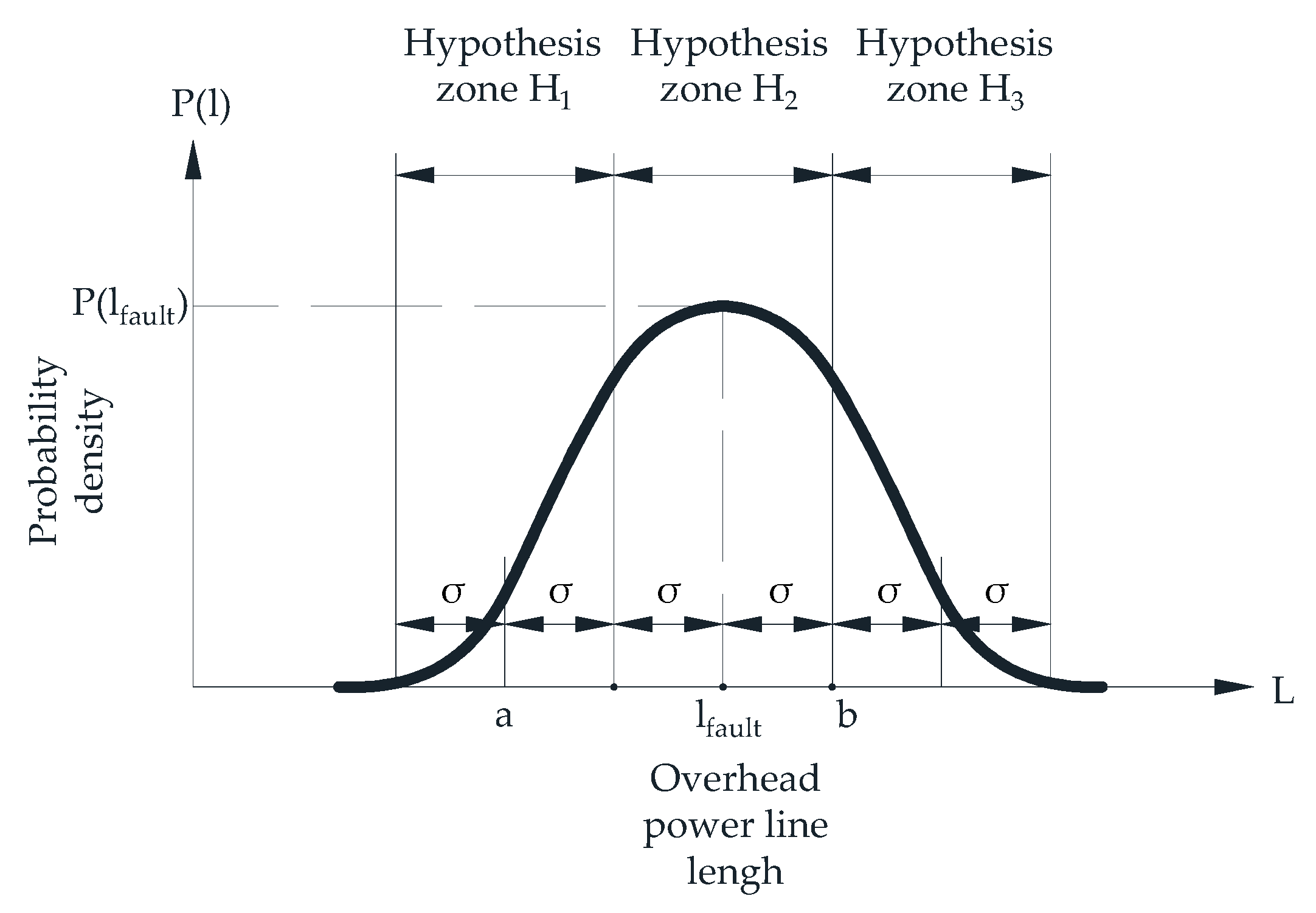
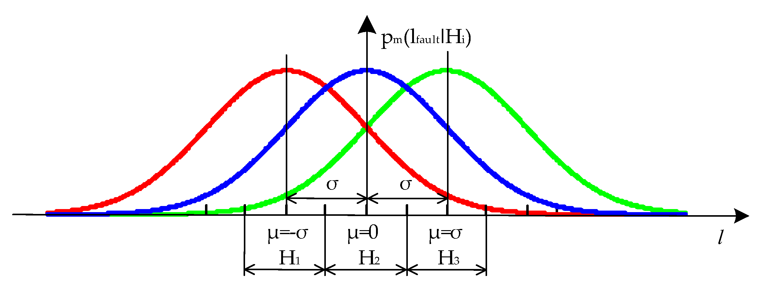
Let us consider a simplified example to characterize the preference and indifference zones for FL. Assume a random distribution of FLs along the OHPL, as shown in Figure 7, resulting from the influence of various random factors. The conformity of the estimated fault distance distribution function to a normal law in FL problems is confirmed in [1]. We assume that the line inspection zone is determined by the “three-sigma” rule [4,30]; that is, it spans an interval of three root mean square (RMS) values of the distribution law in both directions from the estimated FL. For corrective action, this inspection zone is divided into three sections. The objective is to determine, based on consecutive measurements of current and voltage parameters and the subsequent distance calculation, in which section of the OHPL inspection zone the actual fault is located, accounting for distortions caused by the impact of random factors.

The following hypotheses are introduced regarding the OHPL fault location (Figure 7): H₁—when the estimated FL l_fault < a; H₂—when the estimated fault location a < l_fault < b; H₃—when the estimated fault location l_fault > b. Let Δ be some positive value; then the weight functions characterizing the preference and indifference zones are defined as follows:

$${\mathrm{w}}_1({\mathrm{l}}_{\mathrm{fault}})=\left\{\begin{array}{c}0, \mathrm{when}{\mathrm{l}}_{\mathrm{fault}}<\mathrm{a}+\Delta ,\\ 1, \mathrm{when}{\mathrm{l}}_{\mathrm{fault}}\ge \mathrm{a}+\Delta ,\end{array}\right.$$

(3)

$${\mathrm{w}}_2({\mathrm{l}}_{\mathrm{fault}})=\left\{\begin{array}{c}0, \mathrm{when}\mathrm{a}-\Delta <{\mathrm{l}}_{\mathrm{fault}}<\mathrm{b}+\Delta ,\hfill \\ 1, \mathrm{when}\mathrm{there}\mathrm{are}\mathrm{other}{\mathrm{l}}_{\mathrm{fault}}\mathrm{v}\mathrm{a}\mathrm{l}\mathrm{u}\mathrm{e}\mathrm{s},\hfill \end{array}\right.$$

(4)

$${\mathrm{w}}_3({\mathrm{l}}_{\mathrm{f}\mathrm{a}\mathrm{u}\mathrm{l}\mathrm{t}})=\left\{\begin{array}{c}0, \mathrm{when}{\mathrm{l}}_{\mathrm{f}\mathrm{a}\mathrm{u}\mathrm{l}\mathrm{t}}>\mathrm{b}-\Delta ,\hfill \\ 1, \mathrm{when}\mathrm{t}\mathrm{h}\mathrm{e}\mathrm{r}\mathrm{e} \mathrm{a}\mathrm{r}\mathrm{e}\mathrm{other}{\mathrm{l}}_{\mathrm{f}\mathrm{a}\mathrm{u}\mathrm{l}\mathrm{t}}\mathrm{v}\mathrm{a}\mathrm{l}\mathrm{u}\mathrm{e}\mathrm{s}.\hfill \end{array}\right.$$

(5)

The delta (Δ) value determines the ambiguity of decision making and is related to the probability of the FL. The Δ variable is limited by the width of the statistical distribution (see Figure 7).

The zone of preference for accepting hypothesis H₁ is defined by the l_fault point set, for which the condition l_fault < a − Δ is satisfied. The zone of preference for accepting hypothesis H₂ corresponds to the inequality a + Δ < l_fault < b − Δ, and the zone of preference for accepting hypothesis H₃ corresponds to the inequality l_fault > b + Δ.

The indifference zone of hypotheses H₁ and H₂ is defined by the inequality a − Δ < l_fault < a + Δ, the indifference zone of hypotheses H₂ and H₃ is defined by the inequality b − Δ < l_fault < b + Δ, and the indifference zones of hypotheses H₁ and H₃, as well as H₁, H₂, and H₃, are absent.

It is important to note that the weight functions w₁(x), …, w_M(x), which determine risk R(x), have a simple form and can take only two values: 0 or 1. Therefore, the expression for risk (1) is transformed into the following form:

$$\mathrm{R}(\underset{¯}{\mathrm{X}})={\displaystyle {\sum }_{\mathrm{m}=1}^{\mathrm{M}}{\mathrm{P}}_{\mathrm{m}}(\underset{¯}{\mathrm{X}}),}$$

(6)

where the summation is performed only on the m values for which w_m(x) = 1.

Thus, a wrong decision is made only when hypothesis H_m, for which w_i(x) = 1 when i ≠ m, and risk R(x) in this case are equal to the wrong decision probability.

4. Recognition Ability Indicators of Sequential Analysis Algorithms in Overhead Power Transmission Line Fault Location Implementation

In order to form a rational decisive rule, it is necessary to introduce efficiency indicators of the sequential procedure for locating a faulted section. It is reasonable to introduce three main indicators groups: probabilistic, economic, and informational.

The most general probabilistic effectiveness indicator is the conditional probability matrix for M hypotheses, each of which corresponds to a different faulted section within the OHPL bypass zone.

$$‖\mathrm{P}(\left.\mathrm{k}\right|\mathrm{i})‖=‖{\mathrm{P}}_{\mathrm{i}}(\mathrm{k})‖=‖{\mathrm{P}}_{\mathrm{i}\mathrm{k}}‖,$$

(7)

where i, k = 1, …, M and P(k|i) = P_i(k) = P_ik is the conditional decision-making probability on the number of faulted site k under the condition that the damage belongs to site i.

A generalized economic efficiency indicator in classifying faulted areas is the decision error cost matrix ||r_ik||. Based on such matrix, we can introduce the average risk as the average fault cost of a multi-hypothesis sequential analysis procedure.

$$\overline{\mathrm{r}}={\displaystyle {\sum }_{\mathrm{i}=1}^{\mathrm{M}}{\displaystyle {\sum }_{\mathrm{k}=1}^{\mathrm{M}}{\mathrm{r}}_{\mathrm{i}\mathrm{k}}}}\cdot {\mathrm{P}}_{\mathrm{i}}\cdot {\mathrm{P}}_{\mathrm{i}\mathrm{k}}.$$

(8)

It is important to consider that classification errors may have unequal impacts when calculating damage indicators. Clearly, the additional costs associated with an extended inspection of the OHPL—resulting from an incorrect identification of the faulted section—depend on factors such as complex terrain, the equipment used for inspection, and the presence of water obstacles, roads, and access routes to the OHPL. Furthermore, based on statistical data on power line failure rates and potential threats at specific sites, the a priori probabilities (P_i) characterizing the fault likelihood for individual sections may also be unequal.

To reduce the computational cost of implementing classification algorithms, many technical problems [7,9] use cost matrix modifications by introducing unit (simple cost matrices) or diagonal (semi-simple cost matrices) matrices considering that (expression (8)) r_ii = −1 or r_ii = −r_i. Here, negative values of (−1) and (−r_i) indicate “premiums” for correct decisions, and zero values correspond to incorrect decisions. However, the different values of correct decisions may still hold. Expression (8) for the average risk is transformed into the following form:

$$\overline{\mathrm{r}}=-{\displaystyle {\sum }_{\mathrm{k}=1}^{\mathrm{M}}{\mathrm{r}}_{\mathrm{i}}}\cdot {\mathrm{P}}_{\mathrm{i}}\cdot {\mathrm{P}}_{\mathrm{i}\mathrm{i}}.$$

(9)

With equal a priori probability (P_i = 1/M) of fault in OHPL sections, a convenient characterization is the total probability of classification error:

$${\mathrm{P}}_{\mathrm{o}\mathrm{ш}}=({\displaystyle \frac{1}{\mathrm{M}}})\cdot {\displaystyle {\sum }_{\mathrm{i}=1}^{\mathrm{M}}(1-}{\mathrm{P}}_{\mathrm{i}\mathrm{i}}).$$

(10)

Informational classification indicators are based on the current and voltage parameters estimated from emergency event oscillograms and correspond to the degree of uncertainty reduction in the process of decision making about the faulted OHPL. The amount of information to be extracted when locating the i-th OHPL section can be determined by the ratio of a priori P_i and a posteriori P_ii probabilities as follows:

$${\mathrm{I}}_{\mathrm{i}}=\log ({\displaystyle \frac{{\mathrm{P}}_{\mathrm{i}\mathrm{i}}}{{\mathrm{P}}_{\mathrm{i}}}})=\log {\mathrm{P}}_{\mathrm{i}\mathrm{i}}-\log {\mathrm{P}}_{\mathrm{i}}.$$

(11)

The total potential amount of extracted information for all OHPL sections is determined by the formula expression

$${\mathrm{I}}_{\sum }={\displaystyle {\sum }_{\mathrm{i}=1}^{\mathrm{M}}{\mathrm{I}}_{\mathrm{i}}=}{\displaystyle {\sum }_{\mathrm{i}=1}^{\mathrm{M}}\log {\mathrm{P}}_{\mathrm{i}\mathrm{i}}}-{\displaystyle {\sum }_{\mathrm{i}=1}^{\mathrm{M}}\log {\mathrm{P}}_{\mathrm{i}}}.$$

(12)

It is important that the amount of extracted information depends not only on the instantaneous values (parameters) of emergency event oscillograms but also on algorithms for their digital processing. For example, in industrial power supply systems, under conditions of electric PQI deviation from the normative values and recorded current and voltage distortions, it is advisable to introduce special digital processing algorithms to ensure the calculation of the required indicators for locating faulted sections [31].

5. Algorithm and Device for Multi-Hypothesis Sequential Analysis

One way of organizing multi-hypothesis sequential analysis was proposed by Reid [32]. Let x₁, x₂ … be sequence of variables and p_m (x₁, x₂ … |H_i) = p_m(x|H_i) be the joint probability density of x₁, x₂ … under the assumption that hypothesis H_i is true.

Reid’s decision algorithm is based on the generalized likelihood ratio formation at each step m

$${\mathsf{\lambda }}_{\mathrm{m}}(\mathrm{x}\left|{\mathrm{H}}_{\mathrm{i}}\right.)={\displaystyle \frac{{\mathrm{p}}_{\mathrm{m}}(\mathrm{x}\left|{\mathrm{H}}_{\mathrm{i}}\right.)}{\sqrt[\mathrm{M}]{{\displaystyle {\prod }_{\mathrm{k}=1}^{\mathrm{M}}{\mathrm{p}}_{\mathrm{m}}(\mathrm{x}\left|{\mathrm{H}}_{\mathrm{k}}\right.)}}}},\mathrm{i}=1,\dots ,\mathrm{M}.$$

(13)

Those OHPL sections that least fit the fixed set of emergency event oscillogram parameters are sequentially excluded from the analysis when organizing FL. The decisive statistic λ_m(x|H_i) is calculated and compared with the threshold (setpoint) value λ^setpoint_m (x|H_i) of the stopping boundary corresponding to the i-th OHPL section during the sequential analysis procedure. Thus, if λ_m(x|H_j) < λ^setpoint_m (x|H_j), (j = 1, …, M), then a decision is made to continue observation, and the j-th OHPL segment is excluded from the subsequent analysis. The procedure of faulted section identification continues until the last most probable OHPL section remains, which is considered to be faulted.

In performing the sequential procedure process, the stopping boundaries for each of the analyzed OHPL sections are calculated based on the given probabilistic quality indicators of faulted section classification. According to [32], the stopping boundary is defined by the following equality:

$${\mathsf{\lambda }}_{\mathrm{m}}^{\mathrm{п}\mathrm{o}\mathrm{p}}(\mathrm{x}\left|{\mathrm{H}}_{\mathrm{i}}\right.)={\displaystyle \frac{1-{\mathrm{P}}_{\mathrm{i}\mathrm{i}}}{\sqrt[\mathrm{M}]{{\displaystyle {\prod }_{\mathrm{k}=1}^{\mathrm{M}}(1-{\mathrm{P}}_{\mathrm{i}\mathrm{k}})}}}},$$

(14)

where P_ik is the probability of accepting hypothesis H_i, when H_k is valid.

If the condition for the exclusion of one of the OHPL sections from further consideration is met, the total number of analyzed sections is reduced and becomes equal to (M − 1). Subsequently, the stopping limits are recalculated and the multi-hypothesis sequential analysis procedure is repeated until only the most probable faulted section remains.

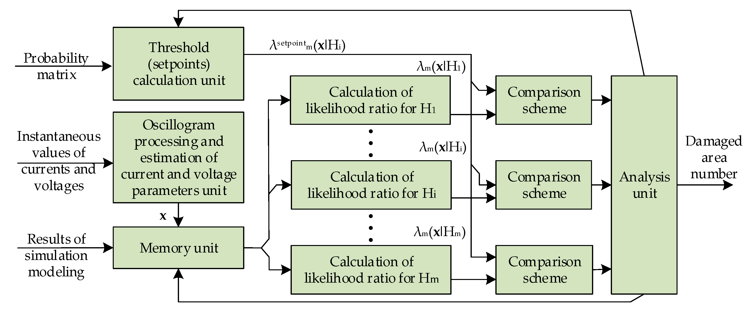
Figure 8 shows the structural diagram of the device which performs multi-hypothesis sequential analysis. The device has a multi-channel structure, and the number of channels M is determined by the number of sections into which the OHPL bypass zone is divided.

The input of the device (Figure 8) receives either instantaneous values or complex quantities of currents and voltages from fault oscillograms. Based on this information, the parameter calculation block computes the components of vector x. This vector can include both values characterizing the faulty OHPL section—such as active and reactive resistances, reactive power, and values of the current distribution coefficient recalculated for the estimated FL—and directly calculated FL values from various algorithms, each with its own systematic and random errors.

Subsequently, in each of the solving statistic calculation blocks, on the basis of vector x, the calculation of likelihood ratios λ_m(x|H_i) peculiar to each of i = 1, …, M OHPL faulted sections is performed (expression (13)). When calculating each of λ_m(x|H_i), the values p_m(x|H_i) and $\sqrt[\mathrm{M}]{{\displaystyle {\prod }_{\mathrm{k}=1}^{\mathrm{M}}{\mathrm{p}}_{\mathrm{m}}(\mathrm{x}\left|{\mathrm{H}}_{\mathrm{k}})\right.}}$ are received from the memory block according to the x values obtained in the parameter calculation block.

It should be noted that simulation modeling is performed in advance of OHPL fault location implementation in order to obtain dependencies p_m(x|H_i) and $\sqrt[\mathrm{M}]{{\displaystyle {\prod }_{\mathrm{k}=1}^{\mathrm{M}}{\mathrm{p}}_{\mathrm{m}}(\mathrm{x}\left|{\mathrm{H}}_{\mathrm{k}})\right.}}$, with the latter being formed for different numbers and combinations of M hypotheses. This is accomplished using specialized software packages, such as Matlab 2024b, PSCAD 5.0, RTDS FX 2.3, or Python 3.13-based ones, which implement multiple simulation modeling with changing variables [10,12]. The probability distribution p_m(x|H_i) can be determined on the basis of statistical operational data, taking into account the errors detected by line crews during OHPL traversals, or it can be determined from the normative values for which the line traversal zone is defined (averaged values for OHPLs of different lengths and voltage classes). Calculations of $\sqrt[\mathrm{M}]{{\displaystyle {\prod }_{\mathrm{k}=1}^{\mathrm{M}}{\mathrm{p}}_{\mathrm{m}}(\mathrm{x}\left|{\mathrm{H}}_{\mathrm{k}})\right.}}$ for different M values are necessary due to the fact that Reid’s algorithm assumes consistent exclusion of hypotheses to make a final decision on the OHPL faulted section.

The calculated likelihood ratio values for each hypothesis λ_m(x|H_i) are fed to the first inputs of M comparison schemes. The second input of each i-th comparison scheme receives the corresponding threshold value λ^setpoint_m(x|H_i) from the threshold calculation block to perform the operation λ_m(x|H_i) < λ^setpoint_m(x|H_i). When the λ_m(x|H_i) value is below λ^setpoint_m(x|H_i) in step m of the sequential procedure, a logic signal is output from the output of the comparison circuit to the analysis unit. In accordance with this signal, the analysis unit decides that there is no fault in the OHPL section numbered i, and the i-th section is excluded from subsequent analysis. Thus, the number of sections is reduced to (M − 1), which leads to the necessity to recalculate λ^setpoint_m(x|H_i) depending on which section was excluded from analysis, as well as changing the dependence involved in the calculation of the likelihood ratio (expression (13)).

To perform the above changes, signals are output from the analysis unit output to the memory unit and the threshold calculation unit inputs. To calculate the threshold values according to expression (14), the threshold calculation block is loaded with the set values of matrix ||P_ik|| determining the detection of the OHPL faulted section with the required indicators of recognizability.

In the processing of emergency event oscillograms, the device (Figure 8) performs the above iterative process and successively decides to exclude hypotheses regarding the OHPL faulted section according to the condition λ_m(x|H_i) < λ^setpoint_m(x|H_i). Then, when the last hypothesis remains, the sequential analysis process stops. The decision that the OHPL fault is located in the corresponding section is made. At the same time, the output of the analysis block of the FL device (Figure 8) provides information about the faulted section (e.g., in the form of a number) within the OHPL bypass zone.

The proposed structure shown in Figure 8 can be implemented as a standalone industrial computer with software implementing the corresponding blocks and digital signal processing. The FL device can also be combined into an intelligent electronic relay protection and automation device. It is installed at the substation, in close proximity to the point where instantaneous current and voltage values are measured.

6. Example of Fault Location Implementation Based on Reid’s Multi-Hypothesis Sequential Analysis Algorithm

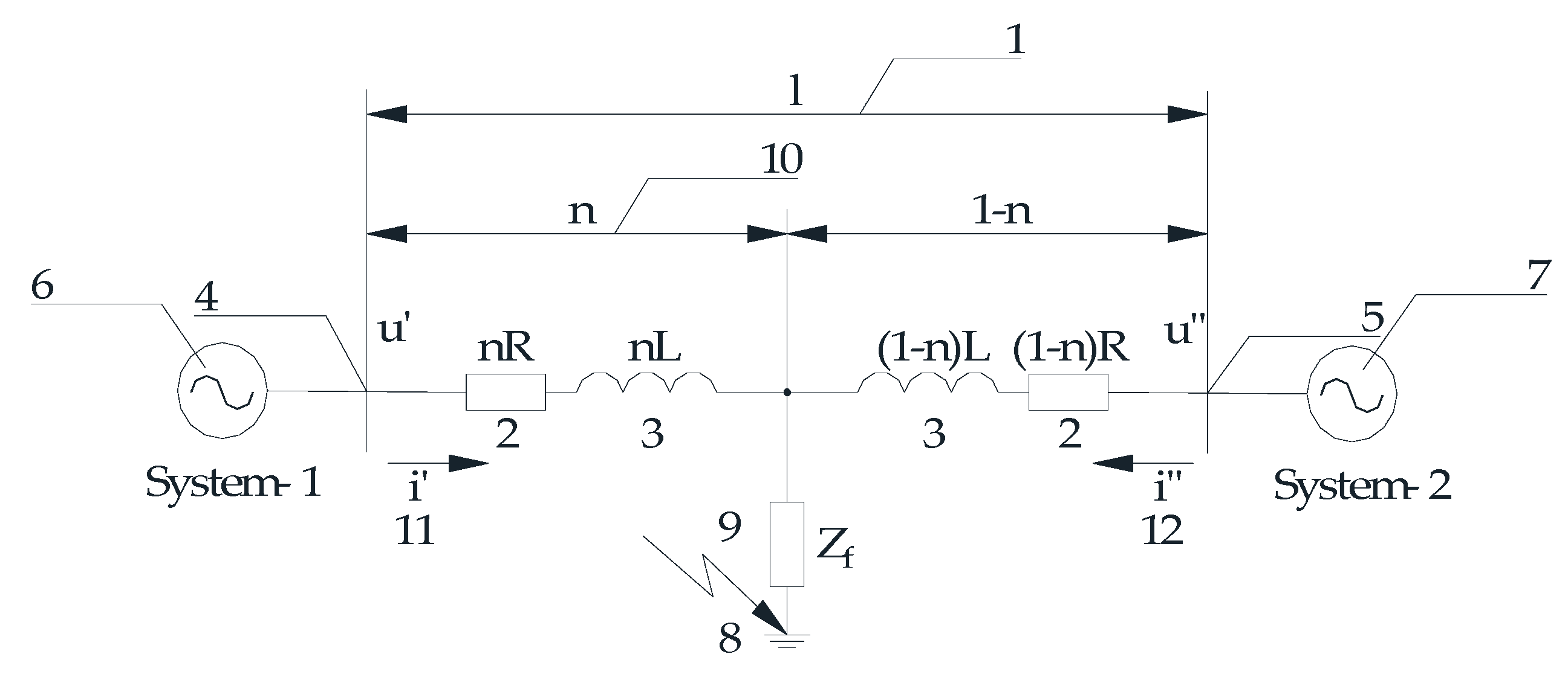
Let us consider the FL procedure implementation in the example of an 110 kV OHPL with a l = 50 km length and two-way power supply (Figure 9).

Figure 9 shows the 110 kV OHPL substitution diagram having length (l) 1, with phase active resistance (R) 2 and inductance (L) 3, connecting busbars 4 and 5 of two systems 6 and 7. The line shows short circuit 8 behind transient resistance (Z_transient) 9 at distance (x = n·l) 10 from one end of the line. When a short circuit occurs on the line, current (i′) flows through the line on the side of busbar 4, and current (i″) flows through the line on the side of busbar 5. In this case, busbars 4 and 5 measure the non-time-synchronized instantaneous values of phase currents (i′_A, i′_B, i′_C), (i″_A, i″_B, i″_C) and voltages (u′_A, u′_B, u′_C), (u″_A, u″_B, u″_C) at the moment of short-circuit.

The relative distance from fault n is determined according to the relation [32]

$$\mathrm{n}={\displaystyle \frac{({\mathrm{u}}^{\prime }(\mathrm{m})-{\mathrm{u}}^{″}(\mathrm{m}))+\mathrm{R}\cdot {\mathrm{i}}^{″}(\mathrm{m})+\mathrm{L}\cdot \frac{{\mathrm{di}}^{″}(\mathrm{m})}{\mathrm{d}{\mathrm{t}}_{\mathrm{m}}}}{\mathrm{R}\cdot ({\mathrm{i}}^{\prime }(\mathrm{m})+{\mathrm{i}}^{″}(\mathrm{m}))+\mathrm{L}\cdot (\frac{{\mathrm{di}}^{\prime }(\mathrm{m})}{\mathrm{d}{\mathrm{t}}_{\mathrm{m}}}+\frac{{\mathrm{di}}^{″}(\mathrm{m})}{\mathrm{d}{\mathrm{t}}_{\mathrm{m}}})}}.$$

(15)

This method of OHPL fault location has rather small errors in calculating the distance from the fault under short-circuit conditions and undistorted (sinusoidal) currents and voltages of the emergency event oscillograms [32].

Suppose that on the side of system 1 (Figure 9), the discrete instantaneous current values i′(m) are distorted by a flicker (e.g., [28]). The distorted current signal i′(m) is illustrated in Figure 10a.

Let us assume that on the side of system 2 (Figure 9), there is a nonlinear load which outputs to the electric network interharmonics. For example simplicity, we consider that the instantaneous current values i″(m) are distorted by an interharmonic of frequency f_{interharmonic} = 135 Hz with amplitude I_{interharmonic} = 0.15·I″ and zero initial phase; see Figure 10b.

Thus, the calculation expression for the FL in the presence of flicker and interharmonic frequency f_interharm = 135 Hz corresponds to the equality

$$\begin{array}{cc}\hfill {\mathrm{n}}_{\mathrm{и}}(\mathrm{m})=& \{({\mathrm{u}}^{\prime }(\mathrm{m})-{{\mathrm{u}}_{\mathrm{interharm}}}^{″}(\mathrm{m}))+{\mathrm{I}}^{″}\cdot [\mathrm{R}\cdot \sin (2\mathrm{\pi }\mathrm{f}\cdot ({\mathrm{t}}_{\mathrm{c}}+\mathrm{m}\cdot {\mathrm{t}}_{\mathrm{d}}))+\mathrm{L}\cdot \cos (2\mathrm{\pi }\mathrm{f}\cdot ({\mathrm{t}}_{\mathrm{c}}+\mathrm{m}\cdot {\mathrm{t}}_{\mathrm{d}}))]+\hfill \\ \hfill & 0.15\cdot {\mathrm{I}}^{″}\cdot [\mathrm{R}\cdot \sin (2\mathrm{\pi }{\mathrm{f}}_{\mathrm{interharm}}\cdot ({\mathrm{t}}_{\mathrm{c}}+\mathrm{m}\cdot {\mathrm{t}}_{\mathrm{d}}))+\mathrm{L}\cdot \cos (2\mathrm{\pi }{\mathrm{f}}_{\mathrm{interharm}}\cdot ({\mathrm{t}}_{\mathrm{c}}+\mathrm{m}\cdot {\mathrm{t}}_{\mathrm{d}}))]\}/\hfill \\ \hfill & \{({\mathrm{I}}^{\prime }\cdot (1-\mathrm{k}\cdot \mathrm{rnd}(\mathrm{m}))+{\mathrm{I}}^{″})\cdot [\mathrm{R}\cdot \sin (2\mathrm{\pi }\mathrm{f}\cdot ({\mathrm{t}}_{\mathrm{c}}+\mathrm{m}\cdot {\mathrm{t}}_{\mathrm{d}}))+\mathrm{L}\cdot \cos (2\mathrm{\pi }\mathrm{f}\cdot ({\mathrm{t}}_{\mathrm{c}}+\mathrm{m}\cdot {\mathrm{t}}_{\mathrm{d}}))]+\hfill \\ \hfill & 0.15\cdot {\mathrm{I}}^{″}\cdot [\mathrm{R}\cdot \sin (2\mathrm{\pi }{\mathrm{f}}_{\mathrm{interharm}}\cdot ({\mathrm{t}}_{\mathrm{c}}+\mathrm{m}\cdot {\mathrm{t}}_{\mathrm{d}}))+\mathrm{L}\cdot \cos (2\mathrm{\pi }{\mathrm{f}}_{\mathrm{interharm}}\cdot ({\mathrm{t}}_{\mathrm{c}}+\mathrm{m}\cdot {\mathrm{t}}_{\mathrm{d}}))]\},\hfill \\ \hfill {\mathrm{u}}^{\prime }(\mathrm{m})=& \mathrm{U}+{\mathrm{I}}^{\prime }\cdot (1-\mathrm{k}\cdot \mathrm{rnd}(\mathrm{m}))\cdot [\mathrm{n}\cdot \mathrm{R}\cdot \sin (2\mathrm{\pi }\mathrm{f}\cdot ({\mathrm{t}}_{\mathrm{c}}+\mathrm{m}\cdot {\mathrm{t}}_{\mathrm{d}}))+\mathrm{n}\cdot \mathrm{L}\cdot \cos (2\mathrm{\pi }\mathrm{f}\cdot ({\mathrm{t}}_{\mathrm{c}}+\mathrm{m}\cdot {\mathrm{t}}_{\mathrm{d}}))],\hfill \\ \hfill {\mathrm{u}}^{″}(\mathrm{m})=& \mathrm{U}+(1-\mathrm{n})\cdot \mathrm{R}\cdot [{\mathrm{I}}^{″}\cdot \sin (2\mathrm{\pi }\mathrm{f}\cdot ({\mathrm{t}}_{\mathrm{c}}+\mathrm{m}\cdot {\mathrm{t}}_{\mathrm{d}}))+0.15\cdot {\mathrm{I}}^{″}\cdot \sin (2\mathrm{\pi }{\mathrm{f}}_{\mathrm{interharm}}\cdot ({\mathrm{t}}_{\mathrm{c}}+\mathrm{m}\cdot {\mathrm{t}}_{\mathrm{d}}))]+\hfill \\ \hfill & (1-\mathrm{n})\cdot \mathrm{L}\cdot [{\mathrm{I}}^{″}\cdot \sin (2\mathrm{\pi }\mathrm{f}\cdot ({\mathrm{t}}_{\mathrm{c}}+\mathrm{m}\cdot {\mathrm{t}}_{\mathrm{d}}))+0.15\cdot {\mathrm{I}}^{″}\cdot \sin (2\mathrm{\pi }{\mathrm{f}}_{\mathrm{interharm}}\cdot ({\mathrm{t}}_{\mathrm{c}}+\mathrm{m}\cdot {\mathrm{t}}_{\mathrm{d}}))],\hfill \end{array}$$

(16)

where k is the number (constant coefficient) characterizing the “distortion depth” by the flicker, rnd(m) is a random number (distributed according to a uniform law in the interval [0; 1], formed at each value of discrete time m), and U is the voltage at the faulted location.

The design parameter values for the example fault location implementation are presented in

Table 2. Values of design parameters.

Parameter	I′ (A)	I″ (A)	f (Hz)	tsampl (s)	L(H)	R (Ohm)	finterharm (Hz)	U(V)	n	k	tc (s)
Value	13,908.15	9030.13	50	0.0025	0.0643	12.5	135	29,323.83	0.5	0.15	0.003

.

Substitution of numerical values according to Table 2 and expression (16) leads to the following results:

-

When m = 20; n_interharm(20) = 0.486; Δx = l·(n − n_interharm) = 50·(0.5 − 0.486) = 0.7 (km);

-

When m = 60; n_interharm(60) = 0.526; Δx = l·(n − n_interharm) = 50·(0.5 − 0.526) = −1.30 (km).

The analysis of the obtained calculation results shows that errors of OHPL fault location can have both positive and negative signs and they are distributed unevenly with respect to the use of different time moments.

Since the OHPL length is l = 50 km, the bypass zone for the accepted FL l_fault is ±10% of the OHPL length or Δl = ±50·0.1 = ±5 (km) relative to the FL.

Taking into account the normal law of OHPL error distribution and the three-sigma rule [30], we can assume that the standard deviation of the normal law of OHPL errors distribution is σ ≈ (2·Δl)/6 = 10/6 = 1.67 (km).

Let us consider a simplified variant of sequential analysis procedure realization with division of the OHPL bypass zone into three sections relative to the FL (Figure 11), corresponding to three hypotheses H₁: μ = −σ; H₂: μ = 0; and H₃: μ = σ.

These hypotheses correspond to the decisions about the correspondence of the FL to the mathematical expectation μ values (Figure 7).

The results of the calculation of the distance from the FL by expression (16) are obtained on the basis of instantaneous current and voltage oscillogram values (Figure 10a,b), i.e., ten consecutive sample l_fault values, which are summarized in

Table 3. Sample values of the distance from the faulted location obtained from alarm event oscillogram instantaneous values.

m	1	2	3	4	5	6	7	8	9	10
Lfault (km)	25.85	24.9	23.7	26.35	24.6	25.6	25.7	27.36	23.75	25.05

. Due to the scatter of sample l_fault values, it is not possible to make an unambiguous decision regarding the fairness of hypotheses H₁, H₂, and H₃.

Note that the mathematical expectation of the sample l_fault values (Table 3) is M[l_fault] = 25.185 (km).

To perform the sequential analysis, the matrix of conditional probabilities (expression (7)) of decision making concerning the faulted site is introduced as

$$‖\mathrm{P}(\left.\mathrm{k}\right|\mathrm{i})‖=‖{\mathrm{P}}_{\mathrm{i}}(\mathrm{k})‖=‖{\mathrm{P}}_{\mathrm{i}\mathrm{k}}‖=‖\begin{array}{ccc}0.70& 0.15& 0.15\\ 0.15& 0.70& 0.15\\ 0.15& 0.15& 0.70\end{array}‖.$$

(17)

The choice of matrix elements should be made by taking into account the operational features of OHPLs, as well as the economic consequences of wrong decisions [1,3].

Let us calculate the thresholds for the sequential multi-hypothesis Reid’s procedure based on the matrix elements in (17):

$${\mathsf{\lambda }}_{\mathrm{m}}^{\mathrm{setpoint}}({\mathrm{l}}_{\mathrm{fault}}\left|{\mathrm{H}}_1\right.)={\mathsf{\lambda }}_{\mathrm{m}}^{\mathrm{setpoint}}({\mathrm{l}}_{\mathrm{fault}}\left|{\mathrm{H}}_2\right.)={\mathsf{\lambda }}_{\mathrm{m}}^{\mathrm{setpoint}}({\mathrm{l}}_{\mathrm{fault}}\left|{\mathrm{H}}_3\right.)=0.353\mathrm{.}$$

(18)

It is reasonable to compute the likelihood ratios λ_m(l_fault|Hi) for each of hypotheses H_i(i = 1, 2, 3) by using a standard Gaussian function,

$$\mathrm{f}(\mathrm{x})=({\displaystyle \frac{1}{\sqrt{2\mathrm{\pi }}}})\cdot \exp \{-{\displaystyle \frac{{\mathrm{x}}^2}{2}}\},$$

(19)

whose tables are given in [33].

In the first step of the sequential analysis, we obtain

l^st_fault(1) = 0.398; p₁(0.398|H₁) = 0.151; p₁(0.398|H₂) = 0.369; p₁(0.398|H₃) = 0.332;

λ₁(0.398|H₁) = 0.151/$\sqrt[3]{0.369\cdot 0.332\cdot 0.151}$ = 0.151/0.2645 = 0.57;

λ₁(0.398|H₂) = 0.369/$\sqrt[3]{0.369\cdot 0.332\cdot 0.151}$ = 0.369/0.2645 = 1.395;

λ₁(0.398|H₃) = 0.332/$\sqrt[3]{0.369\cdot 0.332\cdot 0.151}$ = 0.332/0.2645 = 1.255.

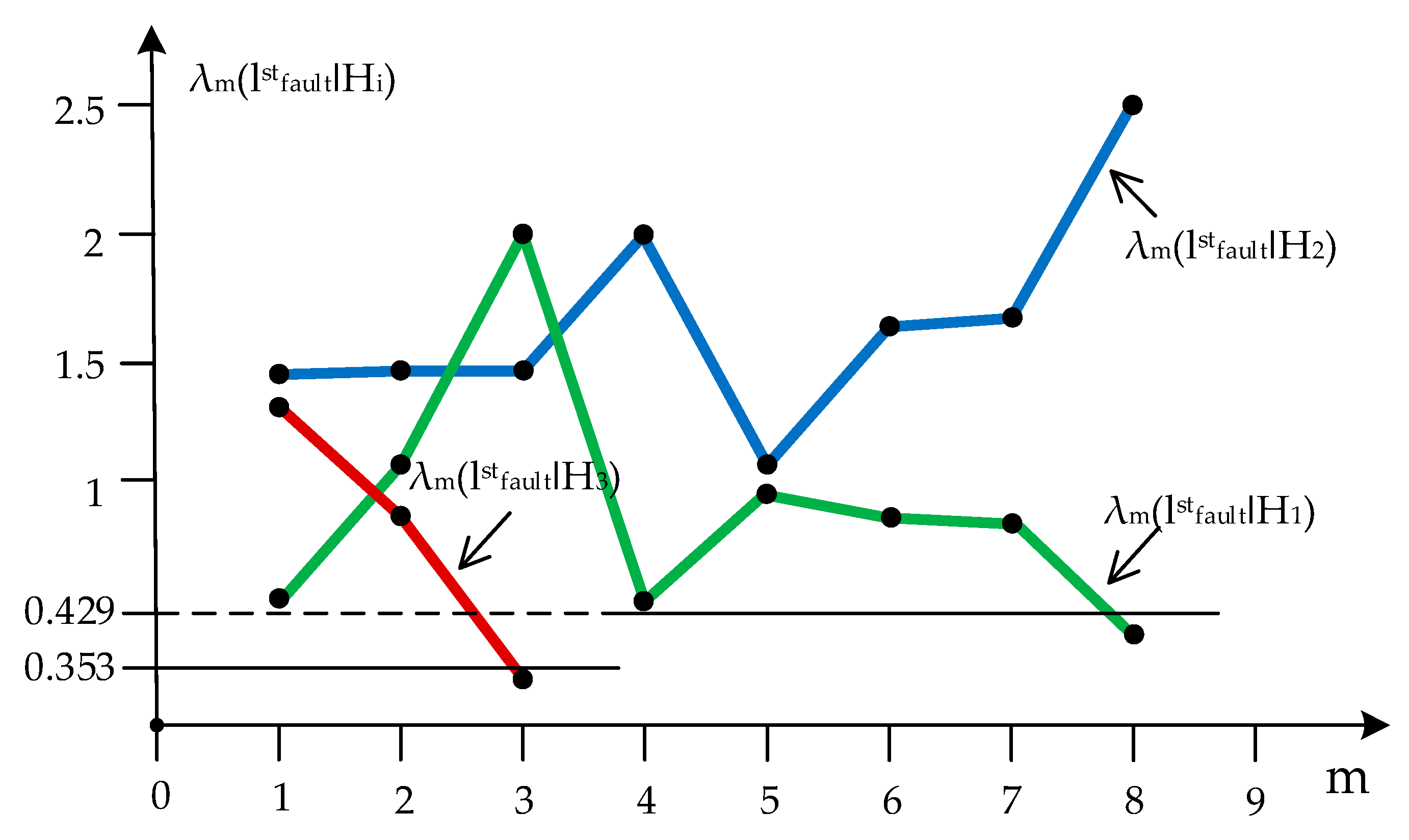
The calculations show (

Table 4. Results of calculations of required values to perform Reid’s sequential analysis.

m	1	2	3	4	5	6	7	8	9	10
pm(lstfault|H1)	0.332	0.2827	0.3964	0.08	0.323	0.1826	0.17	0.0283	−	−
pm(lstfault|H2)	0.369	0.3932	0.2685	0.313	0.3752	0.386	0.381	0.1714	−	−
pm(lstfault|H3)	0.151	0.2012	0.067	−	−	−	−	−	−	−
λm(lstfault|H1)	0.57	1.003	2.059	0.51	0.928	0.689	0.667	0.407	−	−
λm(lstfault|H2)	1.395	1.396	1.395	1.98	1.078	1.457	1.494	2.463	−	−
λm(lstfault|H3)	1.255	0.7117	0.348	−	−	−	−	−	−	−

) that the first step of the sequential analysis does not cause the likelihood ratios calculated for each of hypotheses H₁, H₂, and H₃ to fall below the threshold values, and the sequential analysis procedure continues.

The third step of the sequential analysis eliminates hypothesis H₃, because the likelihood ratio λ₃(−0.889|H₃) is below the threshold value:

$$\mathrm{\lambda }(-0.889\left|{\mathrm{H}}_{\mathrm{3}}\right.) = 0.348 < {\mathrm{\lambda }}^{{\mathrm{setpoint}}_{\mathrm{m}}}(1^{{\mathrm{st}}_{\mathrm{fault}}}\left|{\mathrm{H}}_3\right.) = 0.353.$$

(20)

In the following, the sequential analysis is performed only for two hypotheses, H₁ and H₂. The probability matrix for hypotheses H₁ and H₂ is

$$‖\mathrm{P}(\left.\mathrm{k}\right|\mathrm{i})‖=‖{\mathrm{P}}_{\mathrm{i}}(\mathrm{k})‖=‖{\mathrm{P}}_{\mathrm{i}\mathrm{k}}‖=‖\begin{array}{cc}0.70& 0.30\\ 0.30& 0.70\end{array}‖.$$

(21)

Calculation of threshold values corresponds to the following relations:

$${\mathrm{\lambda }}^{{\mathrm{setpoint}}_{\mathrm{m}}}(1^{{\mathrm{st}}_{\mathrm{fault}}}\left|{\mathrm{H}}_1\right.) = {\mathrm{\lambda }}^{{\mathrm{setpoint}}_{\mathrm{m}}}(1^{{\mathrm{st}}_{\mathrm{fault}}}\left|{\mathrm{H}}_3\right.) = 0.3/0.7 = 0.429.$$

(22)

The implementation of the sequential analysis process using Reed’s algorithm is illustrated in Figure 12.

The analysis of Figure 12 allows us to make the following conclusions:

-

Sequential hypothesis exclusion by Reid’s algorithm leads to the selection of the faulted section in the interval M[l_fault] ± σ/2 = 25.185 ± 0.835 (km);

-

The sequential computational procedure enables decision making concerning the faulted section of the OHPL in eight steps, does not require significant time costs, and practically does not affect the speed of OHPL fault location;

-

Since the initial rejected hypothesis was H₃, it is reasonable to start the OHPL bypass from Section 25.185 ± 0.835 (km) towards system 1 (Figure 9), i.e., the most probable direction of the fault;

-

It is obvious that the decision-making speed during sequential analysis depends on the degree of current and voltage emergency oscillogram distortion, including power quality parameters deviations from standard values.

7. Conclusions

• A new approach to FL is proposed. The method includes OHPL bypass (inspection) zone division into sections with the subsequent implementation of a faulted section location procedure.
• The application of sequential multi-hypothesis analysis enables to adapt the decision-making process concerning the faulted OHPL section to the peculiarities of emergency event oscillogram distortion and the conditions for estimating their parameters.
• The proposed method allows one not only to identify the faulted area under conditions of poor PQIs, i.e., with measurement errors but also to optimize and reduce the bypass zone by using additional data and indicators of recognition ability.
• The results of calculations have shown that the application of sequential analysis practically does not affect the speed of OHPL fault location but provides unambiguity in decision making regarding the faulted section under the influence of random factors.
• The developed method offers potential for application in power districts with inverter-based distributed generation facilities, particularly in grids with poor power quality, for integration into SCADA or protection and automation systems.
• Further research should be focused on adapting the algorithm to various types of interference, developing specialized digital signal processing methods, and creating prototype devices.

References

1. Saha, M.M.; Izykowski, J.; Rosolowski, E. Fault Location on Power Networks; Springer: London, UK, 2010; 437p. [Google Scholar]
2. Papkov, B.; Oboskalov, V.; Gusev, S.; Tavlincev, A.; Mahnitko, A.; Zicmane, I.; Berzina, K. Analysis of the quality problem of electric power and the management of reliability of power supply. In Proceedings of the 10th International Scientific Symposium on Electrical Power Engineering, ELEKTROENERGETIKA 2019, Stara Lesna, Slovakia, 16–18 September 2019; pp. 147–152. [Google Scholar]
3. Grishin, E.; Gryazina, E.; Titov, D.E. Analysis of Risk-Based Diagnostic Scenarios for Overhead Transmission Lines. In Proceedings of the 2023 IEEE Belgrade PowerTech, Belgrade, Serbia, 25–29 June 2023; IEEE: New York, NY, USA, 2023. [Google Scholar] [CrossRef]
4. Kulikov, A.; Ilyushin, P.; Suslov, K.; Filippov, S. Estimating the Error of Fault Location on Overhead Power Lines by Emergency State Parameters Using an Analytical Technique. Energies 2023, 16, 1552. [Google Scholar] [CrossRef]
5. Zhilin, E.V.; Levin, D.D. Analysis of the effectiveness of relative methods for power cable fault detection. iPolytech J. 2025, 29, 363–375. [Google Scholar] [CrossRef]
6. Kulikov, A.; Ilyushin, P.; Loskutov, A.; Filippov, S. Fault Location Method for Overhead Power Line Based on a Multi-Hypothetical Sequential Analysis Using the Armitage Algorithm. Inventions 2023, 8, 123. [Google Scholar] [CrossRef]
7. Zhang, Y.; Xu, Y.; Cui, L. Survey on AI-Assisted Power Transmission Line Fault Detection. Int. J. Crowd Sci. 2025, 9, 139–146. [Google Scholar] [CrossRef]
8. Kulikov, A.; Ilyushin, P.; Loskutov, A.; Filippov, S. Application of Search Algorithms in Determining Fault Location on Overhead Power Lines According to the Emergency Mode Parameters. Algorithms 2023, 16, 189. [Google Scholar] [CrossRef]
9. Simas, F.; Prates, R.; Marotta, A.; Ramos, R.; Cruz, R.; Cardoso, J. Insulator visual non-conformity detection in overhead power distribution lines using deep learning. Comput. Electr. Eng. 2019, 78, 343–355. [Google Scholar] [CrossRef]
10. Kulikov, A.; Ilyushin, P.; Loskutov, A. Enhanced Readability of Electrical Network Complex Emergency Modes Provided by Data Compression Methods. Information 2023, 14, 230. [Google Scholar] [CrossRef]
11. Matikainen, L.; Lehtomäki, M.; Ahokas, E.; Hyyppä, J. Remote sensing methods for power line corridor surveys. ISPRS J. Photogramm. Remote Sens. 2016, 119, 10–31. [Google Scholar] [CrossRef]
12. Kulikov, A.; Loskutov, A.; Bezdushniy, D.; Petrov, I. Decision Tree Models and Machine Learning Algorithms in the Fault Recognition on Power Lines with Branches. Energies 2023, 16, 5563. [Google Scholar] [CrossRef]
13. Lopes, F.V.; Lima, P.; Ribeiro, J.P.G.; Honorato, T.R.; Silva, K.M.; Leite, E.J.S. Practical Methodology for Two-Terminal Traveling Wave-Based Fault Location Eliminating the Need for Line Parameters and Time Synchronization. IEEE Trans. Power Deliv. 2019, 34, 2123–2134. [Google Scholar] [CrossRef]
14. Oswald, P.; Anane, P.O.K.; Huang, Q.; Bamisile, O. Fault Location in Overhead Transmission Line: A Novel Non-Contact Measurement Approach for Traveling Wave-Based Scheme. Int. J. Electr. Power Energy Syst. 2021, 133, 107233. [Google Scholar] [CrossRef]
15. Ngwenyama, M.K.; Le Roux, P.F.; Ngoma, L.J. Traveling Wave Fault Location Detection Technique for High Voltage Transmission Lines. In Proceedings of the 2021 2nd International Conference for Emerging Technology (INCET), Belgaum, India, 21–23 May 2021; pp. 1–6. [Google Scholar] [CrossRef]
16. Zhu, Y.; Fan, X. Fault Location Scheme for a Multi-Terminal Transmission Line Based on Current Traveling Waves. Int. J. Electr. Power Energy Syst. 2013, 53, 367–374. [Google Scholar] [CrossRef]
17. Lachugin, V.F.; Platonov, P.S.; Alekseev, V.G.; Vazyulin, M.V.; Mitrofanov, N.N.; Popov, S.G.; Izmukov, G.N.; Podshivalin, A.N.; Artyunov, S.A.; Klyushkin, N.G.; et al. Field tests of a traveling wave fault location service for overhead transmission lines. Power Technol. Eng. 2022, 55, 783–789. [Google Scholar] [CrossRef]
18. Hung, T.N. Methods for Fault Location in High Voltage Power Transmission Lines: A Comparative Analysis. Int. J. Renew. Energy Dev. 2022, 11, 1134–1141. [Google Scholar] [CrossRef]
19. Kumar, R.; Tripathy, M. A Novel Impedance-Based Fault Locator Algorithm for Transmission Line. Electr. Power Syst. Res. 2023, 224, 109731. [Google Scholar] [CrossRef]
20. Tavoosi, J.; Shirkhani, M.; Azizi, A.; Din, S.U. A Hybrid Approach for Fault Location in Power Distributed Networks: Impedance-Based and Machine Learning Technique. Electr. Power Syst. Res. 2022, 210, 108073. [Google Scholar] [CrossRef]
21. Sharygin, D.; Filatova, G.; Yablokov, A. Locating Faults on Overhead Power Transmission Lines of 110 kV and Above Using Emergency Mode Parameters. In Proceedings of the 2025 7th International Youth Conference on Radio Electronics, Electrical and Power Engineering (REEPE), Moscow, Russia, 4 August 2025. [Google Scholar] [CrossRef]
22. Yablokov, A.A.; Ivanov, I.E.; Panashchatenko, A.V.; Tychkin, A.R.; Kulikov, F.A.; Murzin, A.Y.; Lachugin, V.F. Physical-and-mathematical simulation of impedance-based fault location using synchronized phasor measurements. Power Technol. Eng. 2022, 56, 427–437. [Google Scholar] [CrossRef]
23. Allen, D.E.; Apostolov, A.; Kreiss, D.G. Automated analysis of power system events. IEEE Power Energy Mag. 2005, 3, 48–55. [Google Scholar] [CrossRef]
24. Martynov, M.V. Method for Interval-Based Fault Location on a Power Transmission Line. Russian Patent No. 2720949; IPC H03H 3/40, 15 May 2020. [Google Scholar]
25. Bykadorov, A.L.; Zarutskaya, T.A.; Muratova-Milekhina, A.S. Determination of short circuit location in the electric railway traction. J. Phys. Conf. Ser. 2021, 2131, 042064. [Google Scholar] [CrossRef]
26. Lyamets, Y.Y.; Martynov, M.V.; Voronov, P.I.; Romanov, Y.V. Method for Interval-Based Fault Location on a Power Transmission Line. Russian Patent No. 2639718; IPC H03H 3/40, 22 December 2017. [Google Scholar]
27. Mei, G.; Song, Y. Effect of Overhead Contact Line Pre-Sag on the Interaction Performance with a Pantograph in Electrified Railways. Energies 2022, 15, 6875. [Google Scholar] [CrossRef]
28. EN 50160:2022; Voltage Characteristics of Electricity Supplied by Public Electricity Networks. CENELEC: Brussels, Belgium, 2022.
29. Abraham, W. Sequential Analysis; Dover Publications, Incorporated: Mineola, NY, USA, 2013; 224p, ISBN 978-0486157901. [Google Scholar]
30. Di Paola, G.; Bertani, A.; De Monte, L.; Tuzzolino, F. A Brief Introduction to Probability. J. Thorac. Dis. 2018, 10, 1165–1168. [Google Scholar] [CrossRef] [PubMed]
31. Moravej, Z.; Pazoki, M.; Abdoos, A. Application of Signal Processing in Power Quality Monitoring. In Power Quality—Monitoring, Analysis and Enhancement; IntechOpen: London, UK, 2011. [Google Scholar] [CrossRef]
32. Visyashchev, A.N.; Plenkov, E.R.; Tiguntsev, S.G. Method for Determining the Location of a Short Circuit on an Overhead Power Line Based on Unsynchronized Measurements from Its Two Ends. Russian Patent No. 2508556; IPC G01R 31/08, 27 February 2014. [Google Scholar]
33. Fu, K.S. Sequential Methods in Pattern Recognition and Machine Learning; Academic Press: New York, NY, USA, 1969; 227p. [Google Scholar]
Figure 1. Faulted OHPL replacement scheme.
Technologies 13 00533 g001
Figure 2. Structural diagram of OHPL fault location device.
Technologies 13 00533 g002
Figure 3. The accuracy comparison results of the method in ref. [26] and of the considered FL method in ref. [24].
Technologies 13 00533 g003
Figure 4. Fragment of a two-track section with two-way traction network power supply.
Technologies 13 00533 g004
Figure 5. The structure of aggregate parameter matrix M.
Technologies 13 00533 g005
Figure 6. A working matrix fragment from a simulation experiment.
Technologies 13 00533 g006
Figure 7. An example of the distribution of FLs along an OHPL, taking into account the influence of various random factors.
Technologies 13 00533 g007
Figure 8. A structural diagram of a device implementing a sequential analysis procedure for FL.
Technologies 13 00533 g008
Figure 9. Scheme of 110 kV transmission line single-line replacement.
Technologies 13 00533 g009
Figure 10. Current waveforms distorted by (a) flicker (from the side of system 1; Figure 9) and (b) interharmonics (from the side of system 2; Figure 9) frequency finterharm= 135 Hz.
Technologies 13 00533 g010
Figure 11. Probability distribution of hypotheses pm(lfault|Hi).
Technologies 13 00533 g011
Figure 12. Explanations of the decision-making process in sequential analysis.
Technologies 13 00533 g012