Article

Modeling the Soil Surface Temperature–Wind Speed–Evaporation Relationship Using a Feedforward Backpropagation ANN in Al Medina, Saudi Arabia

by
Samyah Salem Refadah
1,
Sultan AlAbadi
2,
Mansour Almazroui
3,4,
Mohammad Ayaz Khan
5,
Mohamed ElKashouty
6 and
Mohd Yawar Ali Khan
6,*
1
Department of Geography and GIS, Faculty of Arts and Humanities, King Abdulaziz University, Jeddah 21589, Saudi Arabia
2
Hydrogeology and Environmental Geology Program, Saudi Geological Survey, Jeddah 21514, Saudi Arabia
3
Center of Excellence for Climate Change Research/Department of Meteorology, King Abdulaziz University, Jeddah 21589, Saudi Arabia
4
Climatic Research Unit, School of Environmental Sciences, University of East Anglia, Norwich NR4 7TJ, UK
5
Department of Computer Science, College of Science, Northern Border University, Arar 73213, Saudi Arabia
6
Department of Hydrogeology, Faculty of Earth Sciences, King Abdulaziz University, Jeddah 21589, Saudi Arabia
*
Author to whom correspondence should be addressed.
Technologies 2025, 13(10), 461; https://doi.org/10.3390/technologies13100461 (registering DOI)
Submission received: 20 August 2025 / Revised: 26 September 2025 / Accepted: 10 October 2025 / Published: 12 October 2025
(This article belongs to the Special Issue Sustainable Water and Environmental Technologies of Global Relevance)

Abstract

Artificial neural networks (ANNs) offer considerable advantages in predicting evaporation (EVAP), particularly in handling nonlinear relationships and complex interactions among factors like soil surface temperature (SST) and wind speed (WS). In Al Medina, Saudi Arabia, the connections among WS, SST at 5 cm, SST at 10 cm, and EVAP have been modeled using an ANN. This study demonstrates the practical effectiveness and applicability of the approach in simulating complex nonlinear dynamics in real-life systems. The modeling process employs time series data for WS, SST at both 5 cm and 10 cm, and EVAP, gathered from January to December (2002–2010). Four ANNs labeled T1–T4 were developed and trained with the feedforward backpropagation (FFBP) algorithm using MATLAB routines, each featuring a distinct configuration. The networks were further refined through the enumeration technique, ultimately selecting the most efficient network for forecasting EVAP values. The results from the ANN model are compared with the actual measured EVAP values. The mean square error (MSE) values for the optimal network topology are 0.00343, 0.00394, 0.00309, and 0.00306 for T1, T2, T3, and T4, respectively.

1. Introduction

Evaporation (EVAP), an essential element of the hydrological cycle, refers to the change in water from liquid to gas, largely affected by the air temperature, solar radiation, wind speed (WS), and humidity [1]. In arid locations, where water shortages are prevalent, understanding and accurately measuring EVAP rates is critical for the effective management of water resources, ecological conservation, and sustainable development [2,3]. The importance of EVAP studies is heightened by the complex interaction between hydrological processes and climate change—specifically, the modification of the atmospheric water vapor capacity and EVAP rates—which results in the increased occurrence of extreme weather events and significant alterations in precipitation patterns [4,5,6]. The accurate measurement and calculation of EVAP are essential in the design and management of water storage reservoirs, as well as in assessing natural lakes for various applications, including industrial and municipal water supplies, hydroelectric power generation, and irrigation [7]. Disregarding the effects of EVAP can considerably diminish the reservoir storage efficiency, hinder effective water use, and negatively influence economic stability and community welfare.
The temperature of the soil surface is crucial for EVAP, serving as a key catalyst for moisture transport from the soil to the atmosphere. Evapotranspiration is influenced by energy availability, humidity gradients, WS, water accessibility, vegetation traits, stomatal resistance, and soil features such as heat capacity, chemical composition, and albedo [8]. EVAP, an essential element of the water cycle, is profoundly affected by the temperature condition of the soil surface [1]. As solar radiation intensifies, the temperature of the soil surface often rises [9]. This rise in temperature supplies the energy necessary for the transformation of liquid water into vapor, thus augmenting the EVAP rate [10,11]. The impact of surface conditions and characteristics is closely linked to the temperature environment [12]. Due to the varying formulations employed by different models to address surface processes, soil moisture both regulates and is influenced by land–atmosphere water fluxes [13]. EVAP extracts latent heat from the surrounding environment, leading to localized cooling [14]. The influence of irrigation on the surface climate, especially in dry and semi-arid areas, underscores the importance of evaporative cooling in regulating surface temperatures [15].
EVAP is intrinsically linked to the balance between condensation and EVAP, wherein water molecules shift between liquid and vapor states [16]. EVAP occurs when the rate of water molecules leaving the liquid surface exceeds the rate of condensation, a process significantly influenced by WS [17]. The primary function of wind is to remove water vapor that accumulates near the evaporating surface, thereby lowering the vapor pressure and maintaining a concentration gradient that promotes further EVAP [18]. WS acts as a crucial regulator, affecting the rate of water molecule EVAP from a surface into the atmosphere [8]. The relationship between WS and EVAP rates is based on mass transfer principles, where air currents enhance the movement of water vapor from the evaporating surface. Understanding this connection is vital across various fields, such as meteorology, agriculture, and environmental engineering, enabling more accurate predictions of water loss, irrigation management, and climate modeling.
Conventional techniques for estimating EVAP, including empirical formulas and physically based models, often face challenges due to their reliance on oversimplified assumptions and difficulties in accurately representing the complex interactions among various environmental factors. Empirical formulas, such as the Penman–Monteith equation, require precise measurements of several meteorological variables, which may not always be available or reliable in remote or data-scarce regions [19]. In contrast, physically based models need extensive data on soil parameters, vegetation characteristics, and atmospheric conditions, which can be challenging and resource-intensive to obtain. On the other hand, ANN models can identify complex patterns from historical data without requiring a detailed understanding of the underlying physical processes, making them particularly effective for EVAP prediction in data-rich environments.
The estimation of EVAP values using meteorological factors has been the subject of numerous studies [20,21,22,23,24,25,26,27,28], and many of these approaches require data that are not readily accessible. The primary objective of the core documented techniques is to determine a linear correlation among the variables [21]. Nevertheless, various estimation methods indicate that the EVAP process is fundamentally nonlinear [29,30,31]. Many scientists have emphasized the importance of accurate EVAP estimates in hydrologic modeling studies. This criterion may be satisfied by developing enhanced models that incorporate the process’s inherent nonlinearities. Furthermore, techniques that consider a limited number of parameters are essential, as estimations are often needed when meteorological data are insufficient. In recent years, a heightened focus has been placed on modeling nonlinear relationships, and numerous testing approaches for detecting nonlinearities have been developed. However, if the aim of the study is forecasting, merely finding nonlinearities is inadequate; they must be described using a suitable nonlinear model. Regrettably, this concept fails to offer guidance for the model-building process by defining suitable input variables or functional forms for a variety of applications. This challenge makes it appealing to consider a numerical model category that is both theoretical and adaptable [32].
According to Hornik et al. [33], ANNs are semi-parametric regression estimators that are skilled at this task and can approximate almost any calculable function with arbitrary precision. An explicit technique for algorithmically transforming input into output is not necessary for the ANN methodology for system modeling. For the majority of networks, a collection of typical examples of the suggested mapping is adequate. When given input from a training sample, the ANN adjusts to produce the intended result [34,35,36]. Saudi Arabia’s desert environment, characterized by elevated temperatures, minimal precipitation, and intense solar radiation, results in significant EVAP rates, necessitating precise predictions for sustainable water management [37]. This study aims to forecast the complex relationship between WS, SST at 5 cm, SST at 10 cm, and EVAP using an ANN and the FFBP algorithm in Al Medina in Saudi Arabia. This issue is of considerable importance, as few research studies on EVAP prediction have been conducted in Saudi Arabia.

2. Materials and Methods

2.1. Feedforward Backpropagation Algorithm (FFBP)

The feedforward backpropagation (Figure 1) network is fundamental in ANNs, enabling the modeling of intricate relationships in data through a supervised learning framework. This architecture consists of interconnected layers of nodes, facilitating unidirectional information flow from the input layer, through one or more hidden layers, to the output layer, allowing the network to approximate complex functions [38]. Feedforward networks are characterized by the absence of feedback loops, enabling data to flow through the network in a singular, forward direction [39]. This network’s core functionality lies in its ability to learn from data using the backpropagation algorithm, an iterative method that optimizes the network’s internal parameters to reduce the difference between the expected and actual outputs [40,41]. The iterative modification of the connection weights in the network, facilitated by backpropagation, is essential in minimizing the gap between the network’s actual output and the expected output vector, thereby enhancing the representation of critical task domain features [42].
The backpropagation technique, derived from synaptic plasticity in the brain, modifies the weights among neurons in an ANN to enhance performance [43]. The algorithm computes the gradient of the error function concerning each weight in the network and adjusts the weights in the opposite direction of the gradient [44]. This procedure utilizes the chain rule of calculus to effectively calculate gradients for each layer, starting at the output layer and propagating backward to the input layer [45]. The multilayer perceptron network has received considerable attention for its versatility and effectiveness across diverse scientific and technical fields [46]. Enhancements to backpropagation have been investigated to accelerate training and address data overfitting [46]. The backpropagation technique enables multilayer neural networks to identify complex correlations between inputs and outputs, thereby overcoming the limitation of learning only linearly separable vectors, a constraint faced by neural networks such as the perceptron [47].
A feedforward backpropagation network’s architecture generally consists of an input layer for external data, one or more hidden layers for nonlinear transformations of the input, and an output layer for the final prediction [48]. Each layer comprises interconnected nodes or neurons, with links between nodes in adjacent layers possessing corresponding weights that dictate the strength of the connection. Neurons in each layer directly influence the neurons in the subsequent layer. Suppose that the output layer does not produce the desired result. In this case, backpropagation is triggered, transmitting an error signal along the original connection path, which is minimized by adjusting the weights of each neuron [38]. The hidden layers are crucial for identifying complex patterns and nonlinear relationships in the input, allowing the network to represent intricate functions.
The BP technique for a single neuron is explained using the following notations:
t = target output; net = weighted sum to a neuron; n = number of input units to a neuron; E = squared error; y = actual output; winew = ith updated or new weight of a neuron; xi = ith input example/dataset to a neuron; φ(z) = activation function; wi = ith weight of a neuron; ρ = learning rate; b = x0w0, representing the bias value of a network layer.
The weighted sum on any neuron is determined as
n e t = i = 0 n w i x i ,
The activation function is used to calculate the actual output of any neuron as
y = φ (net)
Any nonlinear, differentiable activation function is typically used; the logistic function is a common option and has also been used in the current problem.
φ ( z ) = 1 1 + e z
The gradient descent technique is used by the BP algorithm to reduce the error; this is calculated as
E = 1 2 ( t y ) 2
To minimize the error, for the derivative E w i , which characterizes the rate of change in the error regarding the weights to be computed, the chain rule can be applied as follows:
E w i = d E d y d y d n e t n e t w i
where d E d y denotes the variation in error regarding the output; d y d n e t denotes the variation in the output regarding the weighed sum; and n e t w i denotes the variation in the weighted sum values regarding changes in weights. The values of these derivatives can be computed as
n e t w i = x i
Since
y = 1 1 + e n e t
d y d n e t = d d n e t 1 1 + e n e t = y y 1
d E d y = d d y 1 2 t y 2 = t y
On substituting these values into the equation,
E w i = d E d y d y d n e t n e t w i = t y y y 1 x i
If the logistic function is replaced with another activation function, the phrase “y (y − 1)” will be replaced with the product of the newly chosen activation function. To update the weight wi using the gradient descent approach, a suitable value of parameter ρ, also known as the learning rate or step size, must be chosen. The value of ρ is important since a number that is too small could lead to very sluggish convergence, while a value that is too large could prohibit error convergence. After learning, the weight shift Δwi would be calculated as
Δ w i = ρ E w i = ρ y t φ ( z ) x i
w i n e w = w i + Δ w i
Unless the model meets a preset stoppage threshold, these weights are altered during the NN training process. The terminating criteria are based on a predefined number of epochs or a minimum error value.

2.2. Data Collection

An algorithm in MATLAB (version: R2015a), known as FFBP, was developed for simulation purposes. A nonstop time series dataset covering the daily mean WS, SST (5 cm), SST (10 cm), and EVAP was gathered from January to December for the years 2002–2010. The data used were supplied by the Saudi Arabian Ministry of Environment, Water, and Agriculture (MEWA) and were specific to the Al Medina region (24°31′00.0″ N 39°35′00.0″ E). The patterns were examined in order to comprehend the internal organization of the data, as well as their trends (Figure 2). With respect to EVAP, the line graph (Figure 2a–c) illustrates a direct or indirect link between WS, SST (5 cm), and SST (10 cm).
The shape, symmetry, and dispersion of the huge dataset, as shown by the statistical analysis, are summarized in Table 1. The significant similarity between the mean, median, and mode indicates that the data are in line with a normal distribution. All variables with low standard deviations show that the data are tightly packed around the mean.
The data have positive skewness, except for SST (10 cm), suggesting a rightward shift from the mean and an asymmetrical distribution. With the exception of SST (10 cm), all data exhibit positive kurtosis values, implying a more peaked distribution compared to a normal distribution.

2.3. Data Normalization

Data normalization is an essential preprocessing technique employed across multiple domains, including machine learning, statistics, and database management. The main objective is to transform numerical data into a defined range, often between 0 and 1, or to create a standard normal distribution [49,50,51]. The primary objective of normalization is to lessen the contrary effects of varying scales and units of measurement in raw datasets, hence ensuring the equitable contributions of each feature to subsequent analyses and modeling endeavors [52]. Normalization is crucial for algorithms that are sensitive to feature scaling, such as gradient descent optimization methods employed in neural network training and distance-based algorithms like k-nearest neighbors [53]. Normalization standardizes characteristics to a uniform range, preventing those with elevated values from dominating the learning process, hence enhancing model performance and reliability [54]. Moreover, normalization is essential in enhancing data interpretability, facilitating the extraction of meaningful insights into the relationships among variables within a feature set [55]. Following data collection, each variable was normalized—specifically, SST (5 cm and 10 cm), WS, and EVAP—using the following equation:
X n o r m = X i X min X max X min
where Xmin = minimum value of variable, Xmax = maximum value of variable, and Xnorm = normalized value of observed variable Xi.

2.4. Architecture of Modeled NN

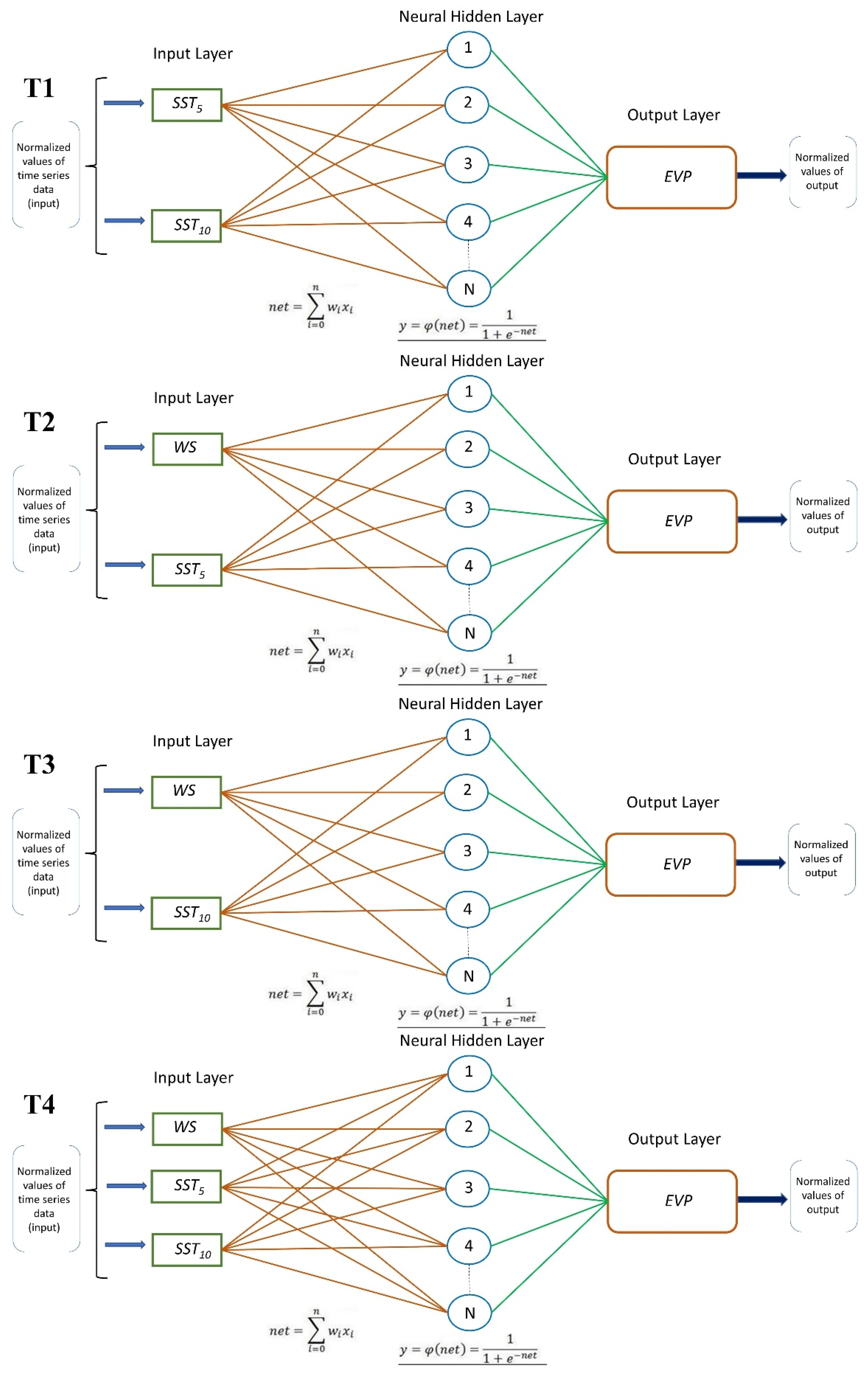
The current network structure involves input, output, and hidden layers. The input layer contains three neurons corresponding to WS, SST (5 cm), and SST (10 cm). Each neuron in the hidden layer is connected to a bias signal with values ranging from 1 to 10. Following model calibration, different combinations of learning rates and hidden-layer neurons were evaluated within the ranges typically employed in artificial neural network research [56,57]. To maintain conciseness, only the results with MSE values nearest to the targeted error threshold are presented, as they most accurately reflect the model’s optimum performance. One neuron in the output layer represents an EVAP value. Four distinct networks (T1–T4) were created based on the existing datasets:
T4: EVAP = f[WS, SST (5 cm), SST (10 cm)];
T3: EVAP = f[WS, SST (10 cm)];
T2: EVAP = f[WS, SST (5 cm)];
T1: EVAP = f[SST (5 cm), SST (10 cm)].
The ANN was trained using normalized time series data. This normalization process adjusts each neuron’s value to fall within a specific range, enhancing network training.
Figure 3 illustrates the neurons presented to the input layer during training and validation across all four networks (T1–T4). Currently, it remains challenging to determine the relationship between the size of the input dataset and the optimal number of neurons in the hidden layers for an effective network topology. In this work, we focused on the mean square error (MSE) and R2, as these metrics are widely recognized and frequently employed in the evaluation of ANN performance. The MSE accurately measures the extent of prediction mistakes, whereas the R2 offers a definitive assessment of the model’s explanatory capacity and goodness of fit. Collectively, they adequately address the aims of this study, which are mostly to illustrate the viability of employing ANNs in the chosen case. Comparable methodologies predominantly utilizing the MSE and R2 have been documented in prior ANN-focused research [58,59,60,61]. The ideal number of layers and related neurons is typically determined in ANN modeling using an enumeration technique focused on lowering the mean square error (MSE), which is also used in this study.
One neuron that reflects the EVAP data makes up the output layer in this investigation. During training and validation, the hidden layer’s neuron count ranges from 1 to 10. The activation function for the output and hidden layers was a sigmoid function.
An enumeration technique was used to optimize the network regarding the number of hidden layers and neurons. Learning rates of 0.01, 0.025, 0.06, 0.08, and 0.1 were tested; based on the mean square error (MSE) criterion, optimal network topologies of 2-6-1 (T1), 2-8-1 (T2), 2-9-1 (T3), and 3-8-1 (T4), with learning rates set at 0.1, 0.1, 0.1, and 0.06, respectively, yielded the best results compared to the other tested configurations. Detailed results and discussions will follow in the next section.

2.5. Datasets

Figure 4 shows the data used for training, validation, and testing in this study. A total of 2774 examples representing the daily WS, SST (5 cm), and SST (10 cm) variables served as the input for training the network. Each of these training examples included the target output in the form of EVAP. From this dataset, 500 examples were allocated for model validation. The network optimization focused on reducing the cumulative mean square error across the entire validation dataset.
After achieving an optimized network, we tested it with 300 examples for EVAP values. These examples were considered solely to test the network’s accuracy and were not used for training or validation.

3. Results

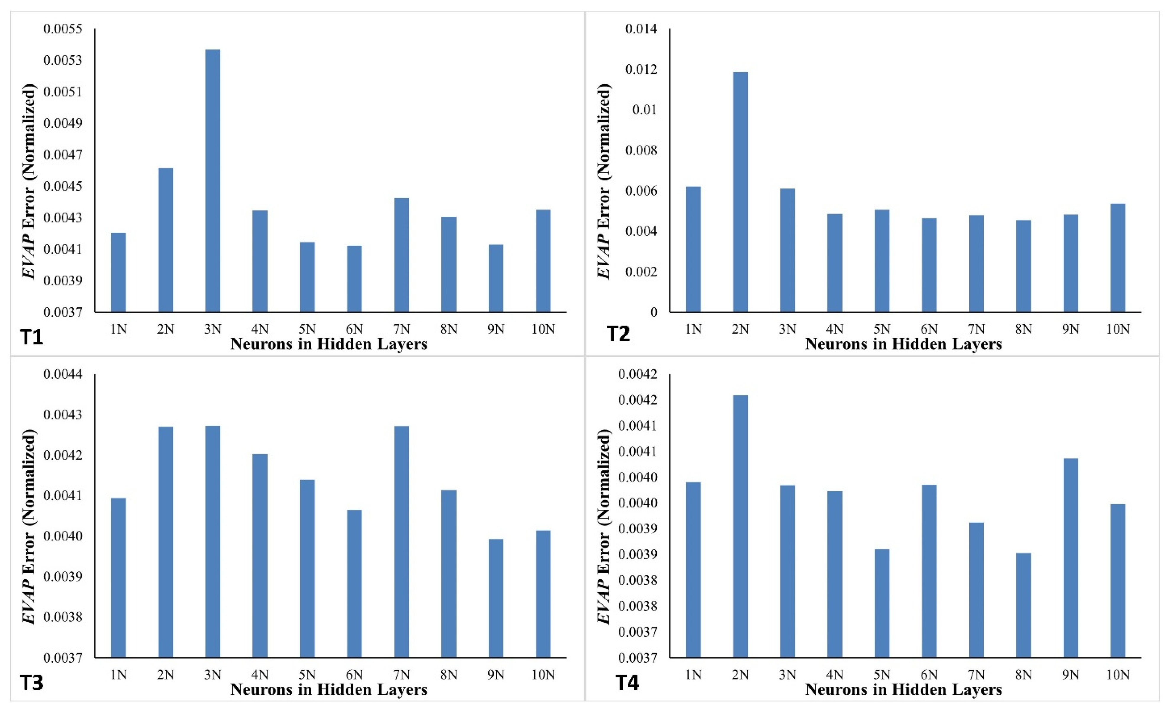
For an optimal network topology, enumeration techniques have been utilized, and the error values for EVAP, in comparison to the observed data, are depicted in Figure 5 for the validation dataset of the four networks (T1–T4). Figure 5 illustrates that T1 demonstrated the smallest error in EVAP with a single-layer network design of six neurons in the hidden layer. The smallest error for T2 and T4 was attained using a single-layer network structure with eight neurons in the hidden layer, but, for T3, this minimum error was achieved with eight neurons in the hidden layer. As of yet, no direct correlation has been identified to forecast the ideal quantity of neurons in the hidden layer; hence, reliance on enumeration techniques is necessary to achieve the optimal network structure.
The optimum topologies identified for predicting EVAP values are 2-6-1 (T1), 2-8-1 (T2), 2-9-1 (T3), and 3-8-1 (T4); these topologies will now be evaluated with varying learning rate values.
Numerous studies indicate that selecting an appropriate learning rate is essential for achieving global minima in errors. The learning rate, a crucial hyperparameter in ANNs, determines the extent of weight changes throughout the training process. Choosing an adequate learning rate is critical, as it significantly impacts the convergence behavior of the training process and the final performance of the trained model [62,63,64]. Hyperparameters, such as the learning rate, greatly affect model selection and neural network architectures, influencing both the efficiency and effectiveness of the learning algorithm [65,66]. An extremely high learning rate can induce instability, leading to divergence in the training process and hindering the network’s convergence to an ideal solution. Conversely, an excessively low learning rate can prolong the training duration, potentially resulting in stagnation within a suboptimal area of the parameter space, thereby hindering the network’s ability to achieve appropriate performance levels [67].
This study evaluated the best network design for T1–T4 using five learning rate values: 0.01, 0.025, 0.06, 0.08, and 0.1. Figure 6 illustrates the fluctuation in the error in the validation dataset corresponding to these learning rate values. Figure 6 clearly demonstrates that the smallest error in EVAP for T1 (six hidden-layer neurons), T2 (eight hidden-layer neurons), and T3 (nine hidden-layer neurons) is achieved with a learning rate of 0.1. The smallest error in EVAP for T4 (with eight hidden-layer neurons) is achieved with a learning rate of 0.06. Consequently, a learning rate of 0.1 is designated for networks T1, T2, and T3 in the test dataset, whereas a learning rate of 0.06 is assigned to T4.
The optimal topology results for networks T1 (six hidden-layer neurons; learning rate 0.1), T2 (eight hidden-layer neurons; learning rate 0.1), T3 (nine hidden-layer neurons; learning rate 0.1), and T4 (eight hidden-layer neurons; learning rate 0.06) from the validation dataset, along with their comparison to experimental values (EVAP), are displayed in Figure 7.
Figure 7 clearly shows that the result patterns obtained using the ANN for the validation dataset closely align with the experimental values. Notably, for T4, which uses three inputs [WS, SST (5 cm), SST (10 cm)], the results are particularly close to the experimental values for EVAP. This indicates that the network has undergone adequate training. As indicated in Table 2, the minimal MSE values were utilized to determine the optimal network configurations. Currently, the ideal network topologies for T1, T2, T3, and T4 are 2-6-1, 2-8-1, 2-9-1, and 3-8-1, with MSE values of 0.00412, 0.00455, 0.00394, and 0.00385, respectively. The R2 values for the four best topologies (T1–T4) were 0.784, 0.766, 0.784, and 0.805, respectively. Therefore, the test dataset is evaluated using the best network topologies for T1 through T4. The targeted MSE was set to 0.0001 for the purposes of this study. However, the average observed MSE across all networks (T1–T4) was approximately 0.003, with an average R2 of 0.750. Although it did not fully reach the specified MSE goal, the performance metrics show that the model remains a reliable approximation of the target function. An R2 score of 0.750 indicates that 75% of the variance in the dependent variable is explained by the model, which is considered an acceptable level of predictive accuracy for complex environmental and geoscientific datasets characterized by inherent noise and heterogeneity. Nevertheless, in the event that raising the number of iterations alone is not sufficient to reach the targeted MSE, it is necessary to take into consideration other techniques, such as making changes to the architecture of the ANN, adjusting the hyperparameters, applying regularization, or incorporating advanced optimization algorithms [57,68].
The test set evaluates the optimal network topologies of 2-6-1 (0.1 learning rate), 2-8-1 (0.1 learning rate), 2-9-1 (0.1 learning rate), and 3-8-1 (0.06 learning rate) for T1, T2, T3, and T4, respectively. Figure 8 displays the neurons in the input and hidden layers during testing for all four networks (T1–T4).
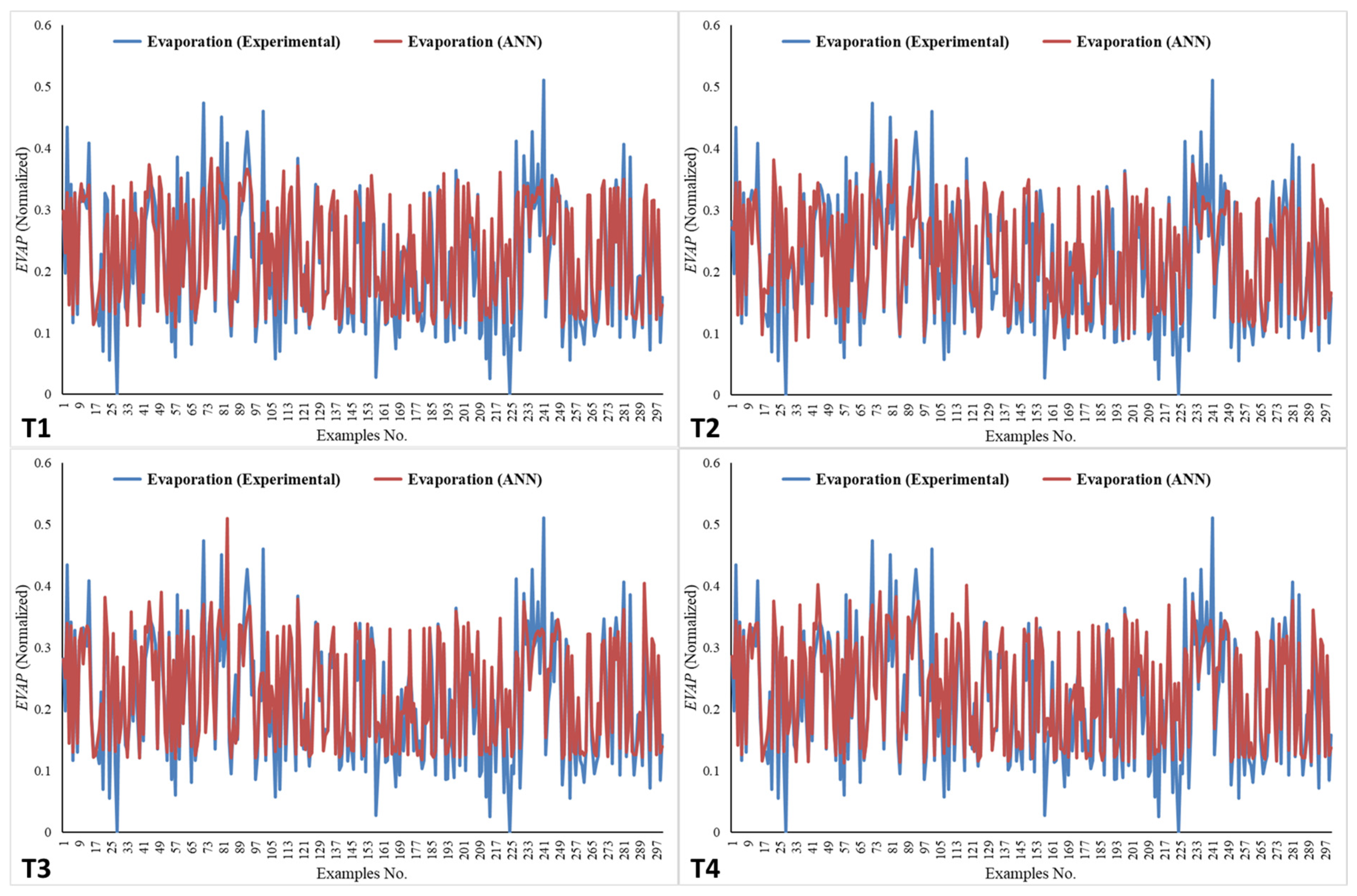
The results for the EVAP values, as predicted by the ANN, alongside the experimental values for the four networks (T1–T4), are illustrated in Figure 9. In Figure 9, the plots effectively demonstrate how the trend in the EVAP values closely aligns with the experimental results, with MSE values of 0.00343, 0.00394, 0.00309, and 0.00306 for T1, T2, T3, and T4, respectively.
The ANN values across all networks closely mirror the experimental EVAP values, with network T4 emerging as the most effective due to its lowest MSE. This suggests a robust correlation between the EVAP rate and the three parameters (WS, SST at 5 cm, SST at 10 cm), facilitating EVAP predictions when any of these parameters are available. For optimal EVAP predictions using ANNs, it is crucial to consider all specified inputs. The ANN model exhibits notable predictive potential; however, it is crucial to acknowledge its limitations, including sensitivity to outliers [69], the unavailability of real-time input data in numerous regions [70], and the inherent risk of excessive dependence on a singular modeling methodology [57]. Subsequent research should focus on these elements by employing rigorous preprocessing methods, integrating real-time data streams, and juxtaposing artificial neural networks with supplementary empirical or hybrid models to improve the reliability and generalization.
All networks (T1–T4) demonstrate their effectiveness in predicting EVAP. This study highlights the advantages of ANN modeling in EVAP prediction, especially in managing nonlinear relationships and the complex interactions among influencing factors like WS and SST.
Such a network model can be utilized to predict EVAP values for ungauged locations. Moreover, if the network is trained on a comprehensive database, it can also forecast values for time series in areas that are challenging to access. The accuracy of this approach can be further enhanced by integrating more experimental data during the network training process. The proposed ANN model, in addition to its methodological demonstration, possesses practical applications in water resource management, such as estimating water losses in reservoirs or distribution systems (e.g., evaporation, seepage, or leakage losses), thereby equipping decision-makers with essential tools for sustainable water allocation and planning [71,72].

4. Conclusions

This study represents the first attempt to predict EVAP using WS and SST data for Al Medina in Saudi Arabia. Four neural network architectures—2-6-1, 2-8-1, 2-9-1, and 3-8-1—with learning rates of 0.1, 0.1, 0.1, and 0.06, respectively, successfully forecasted EVAP values based on time-sensitive data related to WS, SST (at 5 cm), and SST (at 10 cm). While multiple network architectures were created and evaluated, the optimal ANN design was determined through enumeration following the lowest MSE criterion. The proposed topologies delivered satisfactory results for both interpolation and extrapolation data, demonstrating that the network received adequate training. Across all tested topologies, the ANN-predicted values closely followed the trend of the observed values. The results suggest that EVAP prediction can utilize SST at 5 cm and 10 cm depths, either independently or alongside WS. The best prediction of EVAP occurs when three main parameters are used, i.e., SST at both 5 cm and 10 cm together with WS data as inputs, while simulating the network to produce EVAP outputs.
The scope of this study can be broadened to include additional hydrological and meteorological data or their combination. It may also be beneficial to compare other predictive methods, such as fuzzy and neuro-fuzzy techniques, against the ANN approach for these forecasting challenges.

Author Contributions

Conceptualization—S.S.R. and M.Y.A.K.; methodology—S.S.R. and M.Y.A.K.; software—S.S.R., M.A.K. and M.Y.A.K.; validation—S.S.R. and M.Y.A.K.; formal analysis—S.S.R. and M.Y.A.K.; investigation—S.S.R., M.E. and M.Y.A.K.; resources—S.A. and M.Y.A.K.; data curation—S.A., M.A., M.E. and M.Y.A.K.; writing—original draft preparation—S.S.R. and M.Y.A.K.; writing—review and editing—S.A., M.A., M.E. and M.Y.A.K.; visualization—M.A.K. and M.Y.A.K.; supervision—M.Y.A.K.; project administration—S.S.R. and M.Y.A.K.; funding acquisition—M.A. and M.Y.A.K. All authors have read and agreed to the published version of the manuscript.

Funding

This project was funded by the Deanship of Scientific Research (DSR) at King Abdulaziz University, Jeddah, Saudi Arabia under grant no. (DRP-25-155-2025). The authors, therefore, acknowledge with thanks the DSR for the technical and financial support.

Institutional Review Board Statement

Not applicable.

Informed Consent Statement

Not applicable.

Data Availability Statement

Data are contained within the article.

Acknowledgments

This project was funded by the Deanship of Scientific Research (DSR) at King Abdulaziz University, Jeddah, Saudi Arabia under grant no. (DRP-25-155-2025). The authors, therefore, acknowledge with thanks the DSR for the technical and financial support.

Conflicts of Interest

The authors declare no conflicts of interest.

References

  1. Wilson, K.; Hanson, P.J.; Mulholland, P.J.; Baldocchi, D.; Wullschleger, S.D. A comparison of methods for determining forest evapotranspiration and its components: Sap-flow, soil water budget, eddy covariance and catchment water balance. Agric. For. Meteorol. 2001, 106, 153. [Google Scholar] [CrossRef]
  2. Kamai, T.; Assouline, S. Evaporation from Deep Aquifers in Arid Regions: Analytical Model for Combined Liquid and Vapor Water Fluxes. Water Resour. Res. 2018, 54, 4805. [Google Scholar] [CrossRef]
  3. Refadah, S.S.; Khan, M.Y.A. Artificial neural networks for estimating historical daily missing evaporation to support sustainable development in Saudi Arabia. Phys. Chem. Earth Parts A/B/C 2025, 139, 103949. [Google Scholar] [CrossRef]
  4. Kofidou, M.; Stathopoulos, S.; Gemitzi, A. Review on spatial downscaling of satellite derived precipitation estimates. Environ. Earth Sci. 2023, 82, 424. [Google Scholar] [CrossRef]
  5. Dong, Z.; Hu, H.; Wei, Z.; Liu, Y.; Xu, H.; Yan, H.; Khan, M.Y.A. Estimating the actual evapotranspiration of different vegetation types based on root distribution functions. Front. Earth Sci. 2022, 10, 893388. [Google Scholar] [CrossRef]
  6. Hu, H.; Chen, L.; Liu, H.; Ali Khan, M.Y.; Tie, Q.; Zhang, X.; Tian, F. Comparison of the vegetation effect on ET partitioning based on eddy covariance method at five different sites of northern China. Remote Sens. 2018, 10, 1755. [Google Scholar] [CrossRef]
  7. Sadiq, A.A. Measurement and Estimation of Annual Variability of Water Loss at Njuwa Lake Using Class ‘A’ Pan Evaporation Method. Asian Soil Res. J. 2020, 11, 11–21. [Google Scholar] [CrossRef]
  8. Stăncălie, G.; Nert, A. Possibilities of Deriving Crop Evapotranspiration from Satellite Data with the Integration with Other Sources of Information; IntechOpen: London, UK, 2012. [Google Scholar] [CrossRef]
  9. Khamidov, M.; Ishchanov, J.; Hamidov, A.; Shermatov, E.; Gafurov, Z. Impact of Soil Surface Temperature on Changes in the Groundwater Level. Water 2023, 15, 3865. [Google Scholar] [CrossRef]
  10. Jiang, Y.; Fu, P.; Weng, Q. Assessing the Impacts of Urbanization-Associated Land Use/Cover Change on Land Surface Temperature and Surface Moisture: A Case Study in the Midwestern United States. Remote Sens. 2015, 7, 4880. [Google Scholar] [CrossRef]
  11. Jin, M.; Mullens, T.J. A Study of the Relations between Soil Moisture, Soil Temperatures and Surface Temperatures Using ARM Observations and Offline CLM4 Simulations. Climate 2014, 2, 279. [Google Scholar] [CrossRef]
  12. Li, G.; Pan, Y.; Yang, L. Numerical Simulation of the Effects of Water Surface in Building Environment. IOP Conf. Ser. Earth Environ. Sci. 2018, 128, 12072. [Google Scholar] [CrossRef]
  13. la Torre, A.M.; Blyth, E.; Robinson, E.L. Evaluation of Drydown Processes in Global Land Surface and Hydrological Models Using Flux Tower Evapotranspiration. Water 2019, 11, 356. [Google Scholar] [CrossRef]
  14. Jandaghian, Z.; Colombo, A.F. The Role of Water Bodies in Climate Regulation: Insights from Recent Studies on Urban Heat Island Mitigation. Buildings 2024, 14, 2945. [Google Scholar] [CrossRef]
  15. Chen, L.; Dirmeyer, P.A. Global observed and modelled impacts of irrigation on surface temperature. Int. J. Climatol. 2018, 39, 2587. [Google Scholar] [CrossRef]
  16. Brice, J.C. Condensation and evaporation. Solid-State Electron. 1964, 7, 489. [Google Scholar] [CrossRef]
  17. Asano, K. Evaporation and Condensation. In Mass Transfer: From Fundamentals to Modern Industrial Applications; Wiley: Hoboken, NJ, USA, 2006; p. 177. [Google Scholar] [CrossRef]
  18. Hu, H.; Oglesby, R.J.; Marshall, S. The Simulation of Moisture Processes in Climate Models and Climate Sensitivity. J. Clim. 2005, 18, 2172. [Google Scholar] [CrossRef]
  19. Aghelpour, P.; Varshavian, V.; Hamedi, Z. Comparing the Models SARIMA, ANFIS And ANFIS-DE In Forecasting Monthly Evapotranspiration Rates Under Heterogeneous Climatic Conditions. Res. Sq. 2021; preprint. [Google Scholar] [CrossRef]
  20. Jensen, M.E.; Haise, H.R. Estimating evapotranspiration from solar radiation. J. Irrig. Drain. Div. ASCE 1963, 89, 15–41. [Google Scholar] [CrossRef]
  21. Stephens, J.C.; Stewart, E.H. A comparison of procedures for computing evaporation and evapotranspiration. In International Union of Geodynamics and Geophysics; Publication 62; International Association of Scientific Hydrology: Berkeley, CA, USA, 1963; pp. 123–133. [Google Scholar]
  22. Christiansen, J.E. Estimating pan evaporation and evapotranspiration from climatic data. In Irrigation and Drainage Special Conference; ASCE: Las Vegas, NV, USA, 1966; pp. 193–231. [Google Scholar]
  23. Burman, R.D. Intercontinental comparison of evaporation estimates. J. Irrig. Drain. Div. ASCE 1976, 102, 109–118. [Google Scholar] [CrossRef]
  24. Veihmeyer, F.J. Evaporation: Handbook of Applied Hydrology; Chow, V.T., Ed.; McGraw-Hill Book Co.: New York, NY, USA, 1964. [Google Scholar]
  25. Moayedi, H.; Ghareh, S.; Foong, L.K. Quick integrative optimizers for minimizing the error of neural computing in pan evaporation modeling. Eng. Comput. 2022, 38 (Suppl. 2), 1331–1347. [Google Scholar] [CrossRef]
  26. Linarce, E.T. Climate and the evaporation from crops. J. Irrig. Drain. Div. ASCE 1967, 93, 61–79. [Google Scholar]
  27. Azar, N.A.; Kardan, N.; Milan, S.G. Developing the artificial neural network–evolutionary algorithms hybrid models (ANN–EA) to predict the daily evaporation from dam reservoirs. Eng. Comput. 2023, 39, 1375–1393. [Google Scholar] [CrossRef]
  28. Farooque, A.A.; Afzaal, H.; Abbas, F.; Bos, M.; Maqsood, J.; Wang, X.; Hussain, N. Forecasting daily evapotranspiration using artificial neural networks for sustainable irrigation scheduling. Irrig. Sci. 2022, 40, 55–69. [Google Scholar] [CrossRef]
  29. Chen, H.; Huang, J.J.; Dash, S.S.; McBean, E.; Singh, V.P.; Li, H.; Wei, Y.; Zhang, O.; Zhou, Z. Anon-linear theoretical dry/wet boundary-based two-source trapezoid model for estimation of land surface evapotranspiration. Hydrol. Sci. J. 2023, 68, 1591–1609. [Google Scholar] [CrossRef]
  30. Goodarzi, M.; Eslamian, S. Performance evaluation of linear and nonlinear models for the estimation of reference evapotranspiration. Int. J. Hortic. Sci. Technol. 2018, 8, 1–15. [Google Scholar]
  31. Al-Mukhtar, M. Modeling of pan evaporation based on the development of machine learning methods. Theor. Appl. Climatol. 2021, 146, 961–979. [Google Scholar] [CrossRef]
  32. Anders, U.; Korn, O. Model selection in neural network. Neural Netw. 1999, 12, 309–323. [Google Scholar] [CrossRef]
  33. Hornik, K.; Stinchcombe, M.; White, H. Multilayer feed forward networks are universal approximators. Neural Netw. 1989, 2, 359–366. [Google Scholar] [CrossRef]
  34. Khan, M.Y.A. Regional ANN model for estimating missing daily suspended sediment load in complex, heterogeneous catchments. J. Geochem. Explor. 2025, 269, 107643. [Google Scholar] [CrossRef]
  35. Khan, M.Y.A.; Tian, F.; Hasan, F.; Chakrapani, G.J. Artificial neural network simulation for prediction of suspended sediment concentration in the River Ramganga, Ganges Basin, India. Int. J. Sediment Res. 2019, 34, 95–107. [Google Scholar] [CrossRef]
  36. Khan, M.Y.A.; Hasan, F.; Panwar, S.; Chakrapani, G.J. Neural network model for discharge and water-level prediction for Ramganga River catchment of Ganga Basin, India. Hydrol. Sci. J. 2016, 61, 2084–2095. [Google Scholar] [CrossRef]
  37. Şorman, A.Ü.; Abdulrazzak, M.J. Estimation of actual evaporation using precipitation and soil moisture records in arid climates. Hydrol. Process. 1995, 9, 729. [Google Scholar] [CrossRef]
  38. Cao, Y.; Wang, W.; He, Y. Predicting Glossiness of Heat-Treated Wood Using the Back Propagation Neural Network Optimized by the Improved Whale Optimization Algorithm. Forests 2025, 16, 716. [Google Scholar] [CrossRef]
  39. Madhiarasan, M.; Louzazni, M. Analysis of Artificial Neural Network: Architecture, Types, and Forecasting Applications. J. Electr. Comput. Eng. 2022, 2022, 5416722. [Google Scholar] [CrossRef]
  40. Epelbaum, T. Deep learning: Technical introduction. arXiv 2017. [Google Scholar] [CrossRef]
  41. Gershenson, C. Artificial Neural Networks for Beginners. arXiv 2003. [Google Scholar] [CrossRef]
  42. LeCun, Y.; Bengio, Y. Convolutional networks for images, speech, and time series. In The Handbook of Brain Theory and Neural Networks; The MIT Press: London, UK, 1998; p. 255. Available online: https://dl.acm.org/citation.cfm?id=303568.303704 (accessed on 15 July 2025).
  43. Zhao, L.; Zhang, L.; Wu, Z.; Chen, Y.; Dai, H.; Yu, X.; Liu, Z.; Zhang, T.; Hu, X.; Jiang, X.; et al. When brain-inspired AI meets AGI. Meta-Radiol. 2023, 1, 100005. [Google Scholar] [CrossRef]
  44. Zhang, Q.; Wang, T. Deep Learning for Exploring Landslides with Remote Sensing and Geo-Environmental Data: Frameworks, Progress, Challenges, and Opportunities. Remote Sens. 2024, 16, 1344. [Google Scholar] [CrossRef]
  45. Aggarwal, C.C. Neural Networks and Deep Learning; Springer Nature: Cham, Switzerland, 2018. [Google Scholar] [CrossRef]
  46. Huang, Y. Advances in Artificial Neural Networks–Methodological Development and Application. Algorithms 2009, 2, 973. [Google Scholar] [CrossRef]
  47. Sahayam, S.; Zakkam, J.; Jayaraman, U. Can we learn better with hard samples? arXiv 2023. [Google Scholar] [CrossRef]
  48. Skansi, S. Undergraduate topics in computer science. In Introduction to Deep Learning; Springer: Cham, Switzerland, 2018. [Google Scholar] [CrossRef]
  49. Bhanja, S.; Das, A. Impact of Data Normalization on Deep Neural Network for Time Series Forecasting. arXiv 2018. [Google Scholar] [CrossRef]
  50. Djordjević, K.; Jordović-Pavlović, M.I.; Ćojbašić, Ž.; Galović, S.; Popović, M.; Nešić, M.V.; Markushev, D.D. Influence of data scaling and normalization on overall neural network performances in photoacoustics. Opt. Quantum Electron. 2022, 54, 501. [Google Scholar] [CrossRef]
  51. Li, A.; Zhang, W.; Zhang, X.; Chen, G.; Liu, X.; Jiang, A.; Zhou, F.; Peng, H. A Deep U-Net-ConvLSTM Framework with Hydrodynamic Model for Basin-Scale Hydrodynamic Prediction. Water 2024, 16, 625. [Google Scholar] [CrossRef]
  52. Zhao, Y.; Zhang, K.; Guo, A.; Hao, F.; Ma, J. Predictive Model for Erosion Rate of Concrete Under Wind Gravel Flow Based on K-Fold Cross-Validation Combined with Support Vector Machine. Buildings 2025, 15, 614. [Google Scholar] [CrossRef]
  53. Kumari, B.; Swarnkar, T. Stock movement prediction using hybrid normalization technique and artificial neural network. Int. J. Adv. Technol. Eng. Explor. 2021, 8, 874387. [Google Scholar] [CrossRef]
  54. Meira, J. Comparative Results with Unsupervised Techniques in Cyber Attack Novelty Detection. Proceedings 2018, 2, 1191. [Google Scholar] [CrossRef]
  55. Siddiqi, M.A.; Pak, W. An Agile Approach to Identify Single and Hybrid Normalization for Enhancing Machine Learning-Based Network Intrusion Detection. IEEE Access 2021, 9, 137494. [Google Scholar] [CrossRef]
  56. Haykin, S. Neural Networks and Learning Machines, 3rd ed.; Pearson Education: London, UK, 2009. [Google Scholar]
  57. Maier, H.R.; Jain, A.; Dandy, G.C.; Sudheer, K.P. Methods used for the development of neural networks for the prediction of water resource variables in river systems: Current status and future directions. Environ. Model. Softw. 2010, 25, 891–909. [Google Scholar] [CrossRef]
  58. Kisi, O.; Parmar, K.S. Application of least square support vector machine and multivariate adaptive regression spline models in long term prediction of river water pollution. J. Hydrol. 2016, 534, 104–112. [Google Scholar] [CrossRef]
  59. Shamseldin, A.Y. Application of a neural network technique to rainfall–runoff modelling. J. Hydrol. 1997, 199, 272–294. [Google Scholar] [CrossRef]
  60. El-Shebli, M.; Sharrab, Y.; Al-Fraihat, D. Prediction and modeling of water quality using deep neural networks. Environ. Dev. Sustain. 2024, 26, 11397–11430. [Google Scholar] [CrossRef]
  61. Čule, I.S.; Ožanić, N.; Volf, G.; Karleuša, B. Artificial neural network (ANN) water-level prediction model as a tool for the sustainable management of the Vrana Lake (Croatia) water supply system. Sustainability 2025, 17, 722. [Google Scholar] [CrossRef]
  62. Guo, S.; Yang, T.; Gao, W.; Zhang, C. A Novel Fault Diagnosis Method for Rotating Machinery Based on a Convolutional Neural Network. Sensors 2018, 18, 1429. [Google Scholar] [CrossRef]
  63. Ruder, S. An overview of gradient descent optimization algorithms. arXiv 2016. [Google Scholar] [CrossRef]
  64. Smith, L.N. Cyclical Learning Rates for Training Neural Networks. In Proceedings of the 2017 IEEE Winter Conference on Applications of Computer Vision (WACV), Santa Rosa, CA, USA, 24–31 March 2017. [Google Scholar] [CrossRef]
  65. Pfob, A.; Lu, S.-C.; Sidey-Gibbons, C. Machine learning in medicine: A practical introduction to techniques for data pre-processing, hyperparameter tuning, and model comparison. BMC Med. Res. Methodol. 2022, 22, 282. [Google Scholar] [CrossRef]
  66. Prochukhan, D. Implementation of technology for improving the quality of segmentation of medical images by software adjustment of convolutional neural network hyperparameters. Inf. Telecommun. Sci. 2023, 1, 59. [Google Scholar] [CrossRef]
  67. Shaziya, H.; Zaheer, R. Impact of Hyperparameters on Model Development in Deep Learning. In Proceedings of the International Conference on Computational Intelligence and Data Engineering; Lecture Notes on Data Engineering and Communications Technologies; Springer International Publishing: Singapore, 2020; p. 57. [Google Scholar] [CrossRef]
  68. Demuth, H.B.; Beale, M.H.; Jess, O.D.; Hagan, M.T. Neural Network Design, 2nd ed.; Martin Hagan: Stillwater, OK, USA, 2014. [Google Scholar]
  69. Zhang, J.; Zhu, Y.; Zhang, X.; Ye, M.; Yang, J. Developing a Long Short-Term Memory (LSTM) based model for predicting water table depth in agricultural areas. J. Hydrol. 2021, 594, 125734. [Google Scholar] [CrossRef]
  70. Shen, C. A transdisciplinary review of deep learning research and its relevance for water resources scientists. Water Resour. Res. 2018, 54, 8558–8593. [Google Scholar] [CrossRef]
  71. Kisi, O. Evaporation modeling using a neuro-fuzzy approach. J. Hydrol. 2016, 535, 431–438. [Google Scholar]
  72. Nourani, V.; Baghanam, A.H.; Adamowski, J.; Kisi, O. Applications of hybrid artificial intelligence models in hydrology: A review. J. Hydrol. 2020, 580, 124675. [Google Scholar] [CrossRef]
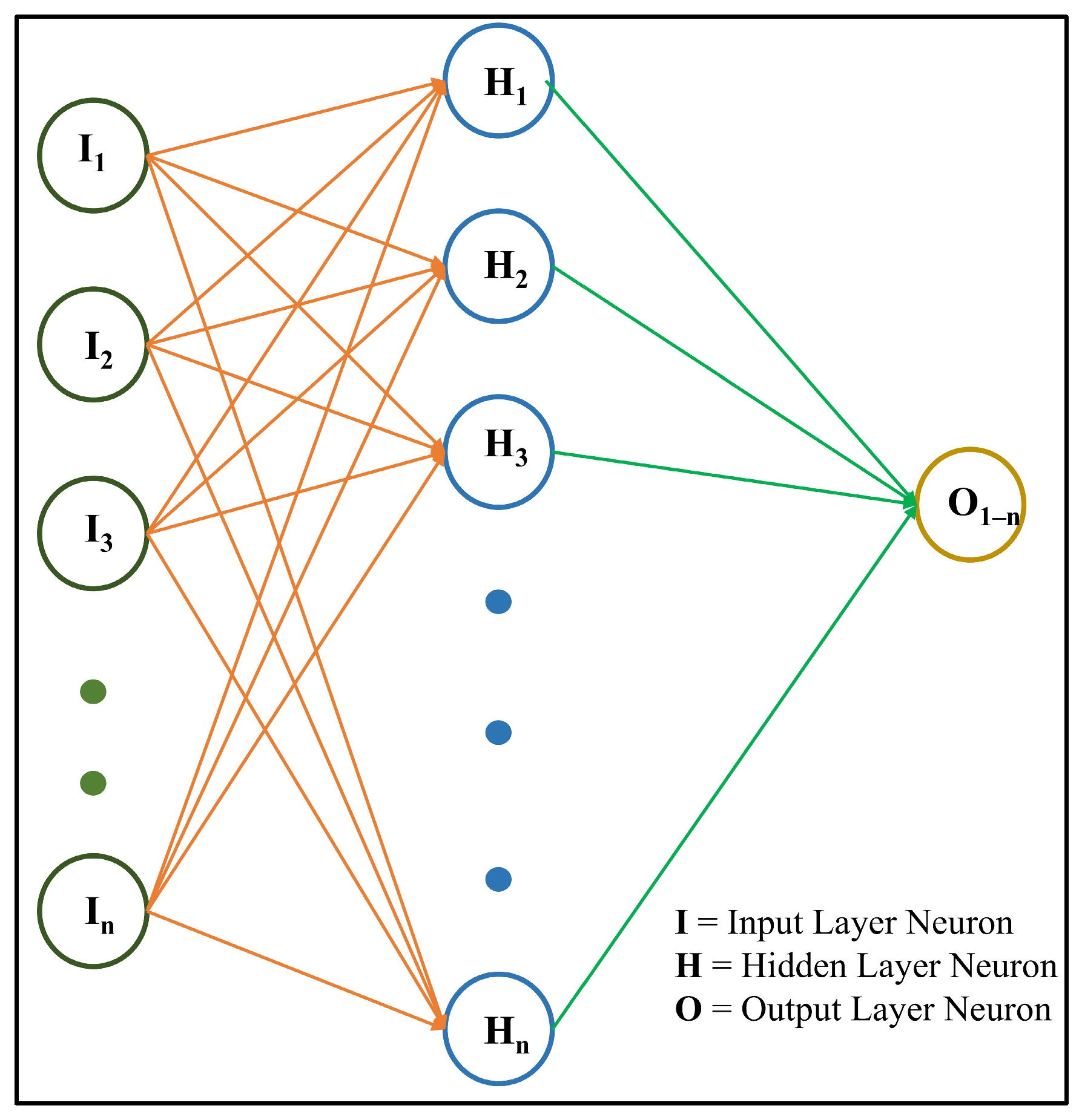
Figure 1. FFBP neural network architecture.
Technologies 13 00461 g001
Figure 2. Relations between (a) WS and EVAP, (b) SST (5 cm) and EVAP, and (c) SST (10 cm) and EVAP.
Technologies 13 00461 g002
Figure 3. Structure of ANN, representing data used for training and validation for the four networks (T1–T4).
Technologies 13 00461 g003
Figure 4. Flowchart of the whole process and information about data used for training, validation, and testing.
Technologies 13 00461 g004
Figure 5. Variation in error values in networks T1–T4 with different numbers of neurons in hidden layers for the validation dataset.
Technologies 13 00461 g005
Figure 6. Variation in error in learning rate values in networks T1 (six hidden-layer neurons), T2 (eight hidden-layer neurons), T3 (nine hidden-layer neurons), and T4 (eight hidden-layer neurons) for the validation dataset.
Technologies 13 00461 g006
Figure 7. Experimental and ANN values for EVAP for networks T1–T4 for the validation set.
Technologies 13 00461 g007
Figure 8. Topology of ANN during the testing stage for four networks (T1–T4).
Technologies 13 00461 g008
Figure 9. Experimental and ANN values for EVAP for networks T1–T4 for the test set.
Technologies 13 00461 g009
Table 1. Statistical depiction of the data values collected at the gauging site.
ParameterWSSST (5 CM)SST (10 CM)EVAP
Mean9.03633.76229.1299.861
SE0.0690.1960.164#VALUE!
Median8.435.230.69.6
Mode741405
SD3.82610.8439.0914.703
Kurtosis8.89219.308−1.221.312
Skewness1.5131.054−0.30.609
Range5219842.843
Min086.80
Max5220649.643
Table 2. The performance and characteristics of the various networks.
Network TopologyT1T2T3Network TopologyT4
R2MSER2MSER2MSER2MSE
2-1-10.7820.004210.7390.006200.7960.004043-1-10.7970.00399
2-2-10.770.004620.0310.011870.6980.005923-2-10.7970.00416
2-3-10.7650.005370.7460.006110.7830.004223-3-10.7980.00398
2-4-10.7750.004350.7490.004850.7960.004153-4-10.7870.00397
2-5-10.7870.004140.7490.005050.7890.004093-5-10.8080.00386
2-6-10.7840.004120.7630.004650.7980.004013-6-10.7970.00398
2-7-10.7810.004430.7340.004780.7660.004223-7-10.8050.00391
2-8-10.7770.004310.7660.004550.7910.004063-8-10.8050.00385
2-9-10.7880.004130.7510.004820.7840.003943-9-10.7990.00404
2-10-10.7840.004350.7470.005370.7870.003963-10-10.8070.00395
Disclaimer/Publisher’s Note: The statements, opinions and data contained in all publications are solely those of the individual author(s) and contributor(s) and not of MDPI and/or the editor(s). MDPI and/or the editor(s) disclaim responsibility for any injury to people or property resulting from any ideas, methods, instructions or products referred to in the content.