Article

Direct Multiple-Step-Ahead Forecasting of Daily Gas Consumption in Non-Residential Buildings Using Wavelet/RNN-Based Models and Data Augmentation— Comparative Evaluation

Faculty of Manufacturing Technologies, Technical University of Kosice, 1, Bayerova St., 08001 Presov, Slovakia
*
Author to whom correspondence should be addressed.
Technologies 2025, 13(10), 435; https://doi.org/10.3390/technologies13100435
Submission received: 18 August 2025 / Revised: 8 September 2025 / Accepted: 25 September 2025 / Published: 28 September 2025
(This article belongs to the Section Information and Communication Technologies)

Abstract

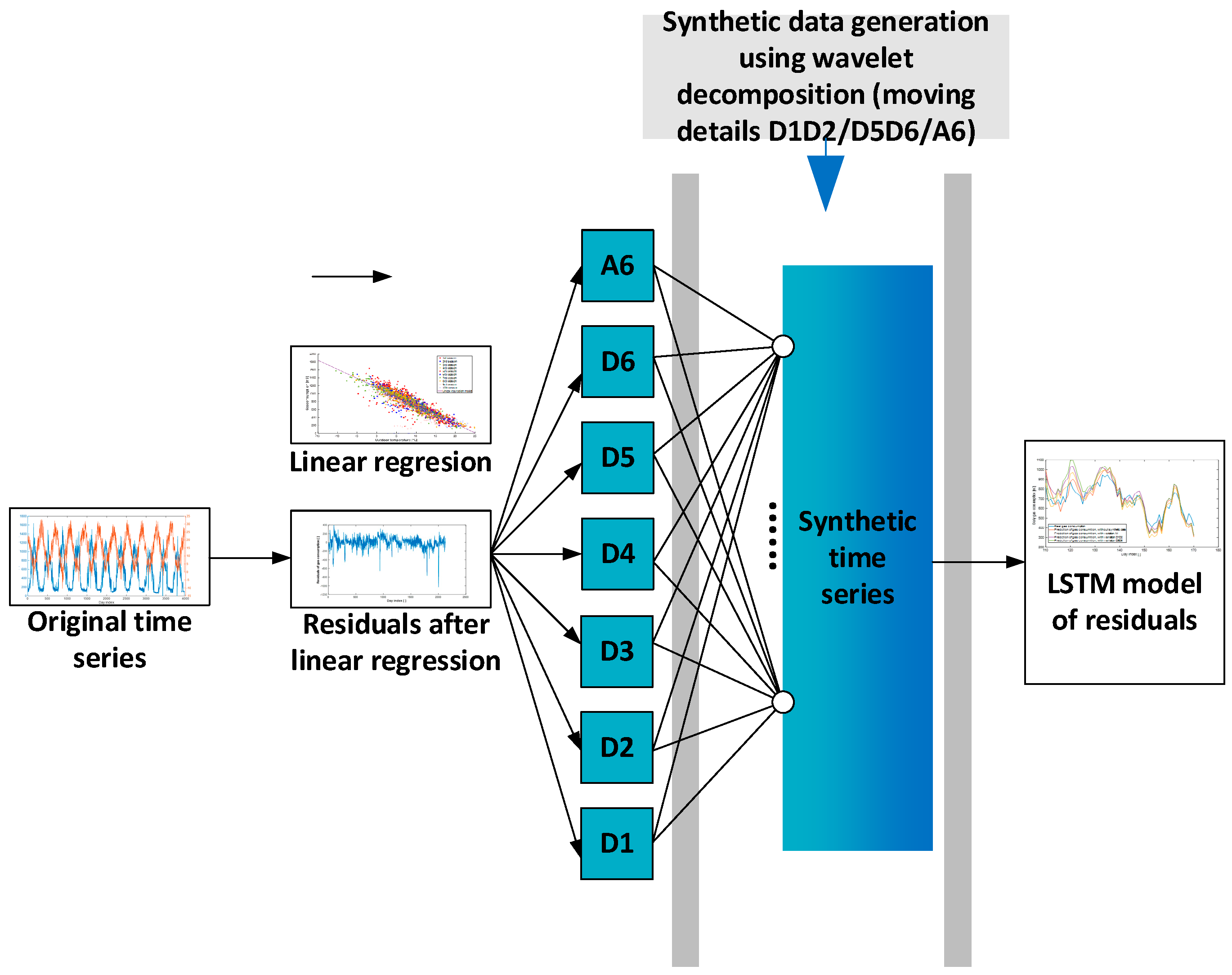
The article focuses on forecasting 7-day daily natural gas consumption for a healthcare facility in Slovakia during the winter season (1 October–30 April). The goal is to optimise operational costs while maintaining user comfort and considering economic and environmental indicators. The prediction is based on historical gas consumption and temperature data from eleven heating seasons (taking into account external factors such as COVID-19 and geopolitical conflicts). Linear regression and counting of residuals, Wavelet decomposition and Long Short-Term Memory (LSTM) neural networks were used. Two approaches were tested: firstly, data augmentation using Wavelet decomposition and creating an LSTM model and secondly, individual prediction of wavelet components by LSTM and combining the best-performing models. The second approach, which forecasted each wavelet component separately and then reconstructed the final prediction, yielded the best accuracy (nMAE = 5.71%, NRMSE = 7.80%). The results showed that using predicted temperatures slightly reduced accuracy. Overall, the Wavelet-LSTM model proved to be the most effective method for forecasting gas consumption in healthcare facilities during winter.

Graphical Abstract

1. Introduction

Short-term forecasting of the consumption of various energy sources has recently been receiving increasing attention. Predicting future consumption or the load on the distribution grid is key to avoid energy waste and to develop effective strategies for consumption management, substitution with alternative sources, and more. The rapid development of smart grids also contributes to an effective solution to this problem. It must be said that forecasting is essential for improving daily life through efficient resource management and service delivery in SMART cities. Such solutions contribute to financial savings and undoubtedly have an impact on environmental issues.

1.1. Literature Review

In the article, the issue of the problem with a 7-day forecast of daily natural gas consumption will be addressed. Therefore, an analysis of gas consumption forecasting, which is particularly relevant in the geographical latitudes of Central and Northern Europe and Asia (where a high level of gasification exists not only in industry but also in households), is proceeded with. Natural gas is used seasonally, with a significant share dedicated to building heating.
Generally, the prediction of electricity consumption or other alternative energy sources cannot be overlooked. This type of forecasting can be approached from the energy supplier’s perspective, as predicting peak loads can help stabilise the grid [1,2,3]. On the other hand, from the perspective of the electricity consumer, the goal is to optimise costs and maintain financial limits on energy prices [4]. Some authors have included in their model development factors that are assumed to influence the final model, such as meteorological conditions or public holidays. Others considered only the workday/weekend mode. This is especially relevant for electricity consumption, which occurs year-round—both during the winter season (for heating) and the summer season (for air conditioning).
Several authors have addressed the gas consumption issue, and many of the existing studies are summarised and offer an overview of the various approaches to forecasting gas consumption.
First, studies such as [5] from 2021 or works [6] and [7] should be mentioned. Recently, however, the focus has mainly shifted toward comparative studies, where the quality of a model is evaluated through comparison metrics.
According to the literature [5], the history of natural gas consumption forecasting can be divided into four main stages: the initial stage (up to the 1970s), the conventional stage (up to 1992), the artificial intelligence stage (1992–2006), and the complex stage (2006–present). If we focus on the most recent years of research, there has been a significant surge in development since 2006. On one hand, this growth has been driven by increased awareness of energy savings, as well as support for green economy concepts. On the other hand, it has been enabled by advances in computational capacity—particularly the introduction of multilayer neural networks and the concept of deep learning.
The Long Short-Term Memory (LSTM) model, a specialised form of a recurrent neural network (RNN), has become the most popular deep learning model [5,8]. It effectively addresses the vanishing gradient problem typical of RNNs, as each LSTM cell retains information about previous states, thereby improving the connections between time steps. Statistical analysis of data characteristics, models, and forecasting results shows that time series models are the most suitable for long-term predictions, achieving the lowest mean absolute percentage error. In contrast, artificial intelligence-based models perform the best for medium- and short-term forecasting. Among these, artificial neural network models showed the best results for medium-term forecasting, while support vector regression models were the most effective for short-term forecasting [5].
Next, the publication by the authors [9], in which a statistical analysis of the state of the studied problem up to the year 2019 was conducted, would be mentioned.
Another review paper [10] presents an analysis of statistical and machine learning methods used in simulating the energy performance of buildings. It not only presents and analyses theoretical aspects but also includes selected published studies. The categorisation largely corresponds to the historical development described in work [5], but it also includes a description of input and output data, modelling specifics, and key results.
The statistical learning methods discussed include: linear prediction models, generalised linear models (GLMs), linear mixed-effects models, Bayesian approaches, and time series analysis. This section of the manuscript is supplemented by a review table summarising studies that focus on linear and Bayesian models, as well as (S)ARMA and (S)ARIMA models.
In the category of machine learning methods, the authors [10] include: deep neural networks (deep learning), including deep feedforward, recurrent, and convolutional neural networks; support vector machines (SVMs); and ensemble learning models (e.g., Random Forest, Gradient Boosting). Each of these techniques is supported by a review of relevant research studies. The included publications frequently focus on comparing the use and effectiveness of various methods or approaches while also varying in terms of source data (climate and meteorological influences), sample size (small- or medium-scale gas consumers or even national energy planning), and forecast horizon.
If we follow the historical development and classification of methods as outlined in works [5] and [10], then from the vast body of literature, we can highlight a few selected studies.
Some studies focus on a statistical approach to solving the problem. The development of smart gas meters has enabled the collection of daily natural gas consumption data, which can be used to build and improve methods and models for consumption forecasting. In articles [11,12], the authors address the development of a short-term prediction model for total natural gas consumption, using only two input variables: daily natural gas consumption and average daily temperature. The data were collected from the distribution network side, based on over 3300 smart gas meters, recorded over a six-month period. The problem was approached statistically, with the models developed using Python programming. The model calculated predictions based on three parameters (shape, location, and scale). The best results were achieved using a two-day rolling average temperature in a consumption scenario of up to 250 m3 per day, yielding a MAPE value of 7.26%.
Advantages of ARMA and ARIMA models include their ability to capture important characteristics of time series data, such as long-term trends and recurring patterns, as well as their user-friendliness and ease of implementation. However, these models are less effective when dealing with time series exhibiting seasonal patterns—unless extended with seasonal components, such as Seasonal ARMA (SARMA) or Seasonal ARIMA (SARIMA). They are also very sensitive to outliers and tend to perform poorly in modelling structural breaks or turning points in the time series.
Time series analysis and the use of ARIMA and SARIMA models in hybrid models are discussed in [13], which concludes that hybrid models combining two or more machine learning techniques are advantageous. Specifically, a hybrid model combining ARIMA and evolutionary algorithms (EAs) can leverage ARIMA to capture periodicity and linear trends, while EAs effectively model nonlinear residual components.
Furthermore, in [14], the authors compare various models for monthly forecasting of natural gas production and consumption using cross-correlation functions and analyse the relationship between exogenous variables. The performance of the proposed model was also compared to the SARIMA (p, d, q) * (P, D, Q)s model. The results based on the RMSE and MAPE indicators highlight the superiority of the best-performing model. Using this approach, monthly natural gas production and consumption in the USA are forecasted up to 2025. If the seasonal trend continues, natural gas production in the USA is expected to increase by 16% and consumption by 24% by 2025. This study provides valuable insights for national energy planning, policymakers, and energy strategy development.
Machine learning (ML) is a subfield of artificial intelligence (AI) that uses historical data to create and train algorithms and models capable of estimating or predicting outcomes without the need for explicit programming. The goal of machine learning is to achieve accurate predictions based on past experience. The learning process typically involves training a model on a large dataset, validating its performance, and then applying it to new, previously unseen data. Over the past few decades, machine learning (ML) has been increasingly used in building research and has shown potential for improving its performance [10].
The use of deep learning and comparison with other models was addressed, for example, in [15]. The study examined the possibilities of hourly natural gas demand forecasting and compared statistical methods with deep learning techniques to evaluate their predictive accuracy across five different locations in Spain. Hourly forecasting achieved an adjusted coefficient of determination (R2) of approximately 0.99 and a MAPE below 2.7%. Stepwise Multiple Linear Regression (SMLR) provided high predictive accuracy (MAPE: 3–10%) at four locations. The Multilayer Perceptron (MLP) produced fewer extreme predictions (517 cases) with similar accuracy (MAPE: 3–11%). Long Short-Term Memory (LSTM) models also demonstrated good predictive accuracy (MAPE: 3–13%) and effectively handled extreme values. Other methods generally yielded less promising results but may be suitable for specific locations.
Different combinations of LSTM and Wavelet decomposition were studied in [16] and [17]. Reference [16] focuses on natural gas consumption prediction and the incorporation of influencing factors into prediction models. This study proposes a natural gas consumption prediction model based on feature optimisation and incremental LSTM. The Mean Absolute Percentage Error (MAPE) was used as the evaluation metric. Since the analysis covered 7 industrial zones and 6 residential areas, the research primarily aimed to identify factors affecting gas consumption—such as temperature, humidity, local holidays, consumer structure, and national policy approaches—and their impact on prediction errors across various models. This was approached from the consumer side. The proposed method demonstrated exceptional performance in daily gas consumption prediction for the city of Wuhan during the period from 2011 to 2024. Specifically, it achieved low average prediction errors of 0.0556 for the 10 coldest (heating) days.
A similar issue to the one addressed in our work is discussed in [17]. The rapid development of the gas industry in China has created a need to secure and satisfy the growing population demand for gas and to design gas storage facilities for peak regulation. The article proposes a new hybrid model that integrates three methods, LMD (Local Mean Decomposition), WTD (Wavelet Threshold Denoising), and LSTM (Long Short-Term Memory), for short-term gas consumption forecasting. It analyses the influence of different temperatures and forecasting time lengths (FTLs) on the accuracy of the LMD-WTD-LSTM model. In this study, the LMD-WTD-LSTM model is applied to predict the daily gas load in London.
And finally, CNNs and various combinations, comparisons, and hybrid models are discussed in, e.g., [7,18,19,20,21].
In [18], the authors focus on the German environment. The goal is accurate and reliable short-term forecasting of natural gas demand and supply, which is crucial for stable energy delivery. They proposed a hybrid prediction model that combines a Functional AutoRegressive (FAR) model and a Convolutional Neural Network (CNN). They performed short-term hourly flow predictions for 92 distribution nodes in a German high-pressure gas network. The results show that the proposed FAR-CNN model achieves high and stable accuracy across different types of nodes. For P-nodes (industrial nodes) and M-nodes (urban nodes), which have more complex consumption structures and dynamics, the FAR-CNN model outperformed all alternative models. For P-nodes, the improvement in the MAPE ranged from 3.6% up to 128.5% compared to other models, while for M-nodes, the improvement was even more significant—from 4.5% to 340.5%.
The use of LSTM is addressed by the authors of [19]. They propose a three-layer neural network prediction model that can extract key information from input factors and improve the weight optimisation mechanism within the Long Short-Term Memory (LSTM) network to effectively predict short-term consumption. The performance and robustness of the proposed model were validated on datasets with varying degrees of fluctuation and complexity. Compared to traditional two-layer models (CNN-LSTM and LSTM-ATT), the Mean Absolute Range Normalised Error (MARNE) improved by more than 16% in Athens and by more than 11% in Spata.
The authors of [19] also analyse the possibilities of using machine learning algorithms, neural networks, and two regression algorithms, Multiple Linear Regression (MLR) and Random Forest, for natural gas consumption prediction. The results obtained from MLR, Random Forest, and Deep Neural Networks (DNNs) show that the Random Forest algorithm achieves the best prediction results for the tested input data. However, differences in accuracy between the algorithms were not significant and were influenced by factors shaping natural gas demand, as well as varying prediction accuracy depending on the forecast horizon. They performed a one-day prediction on a sample from a medium-sized Polish city.
A similar goal was set by the authors of [20]. The basis of intelligent natural gas supply planning is an accurate prediction of natural gas consumption (NGC—Natural Gas Consumption). However, its volatility brings difficulties and challenges for precise consumption forecasting. To address this problem, an improved model was developed that combines the Improved Sparrow Search Algorithm (ISSA), Long Short-Term Memory (LSTM), and Wavelet Transform (WT). The data were collected in China. The prediction quality was compared with the results obtained by other methods. The ISSA-LSTM method offered the best result with a MAPE of 6.26%, while LSTM had a MAPE of 9.93% and XGBoost 18.94% [20].
The authors of [20] compared traditional statistical models such as ARIMA, SARIMA, and SARIMAX and concluded that these models achieve worse predictive accuracy compared to the proposed models, mainly due to their requirement for stationary input data. However, the tested methodology can also work with non-stationary data, which increases its applicability in real-world scenarios. The best results were provided by a machine learning model that utilised multiple Light Gradient Boosting sub-models. Deep learning models achieved intermediate results—better than traditional models but slightly weaker than multi-model machine learning approaches. The experimental results indicate a significant improvement in accuracy achieved by machine learning and deep learning models, leading to a substantial reduction in the mean absolute error.
A contribution of the research is the introduction of a machine learning and deep learning approach to multi-output time series forecasting and, notably, the presentation of a new evaluation metric called Change Point Neighbourhood Error (CPNE). The goal of this metric is to provide a specific measure of prediction accuracy of the proposed models in parts of the time series where data breaks or drifts occur. Furthermore, the authors emphasised the importance of data preprocessing in the deep learning methodology, which significantly contributed to the overall performance of the model.
Reference [22] proposes a novel natural gas consumption forecasting method called DCSDNet, based on dual convolution and seasonal-trend decomposition. First, seasonal-trend decomposition is applied to the original time series to obtain seasonal components, trend, and residuals. Then, dual convolution is performed on the trend and residuals, followed by the use of a self-attention module. Seasonal components and the output of the self-attention module are then reseasonalized. An autoregressive component is introduced into the model to ensure sensitivity to the input scale.
To remove noise, singular spectrum analysis (SSA) is often incorporated into hybrid models. However, SSA does not provide good results when the time series has a high noise level. Considering this fact, the authors of [23] proposed an improved SSA method (ISSA) that modifies the subseries selection method during the reconstruction phase of SSA. Combined with Long Short-Term Memory (LSTM), a new hybrid model ISSA-LSTM was developed. To validate the robustness and performance of ISSA-LSTM, historical datasets from four representative cities located in three climate zones were collected for training and testing the model. Subsequently, a comparative analysis of ISSA-LSTM with five advanced models was conducted. ISSA-LSTM achieved the best results, with MARNE values for the cities as follows: London (temperate zone), 4.68%; Melbourne (subtropical zone), 5.72%; Karditsa (subtropical zone), 5.76%; Hong Kong (tropical zone), 14.10%.

1.2. Research Objective

To summarise this overview, the literature review reveals two main approaches to natural gas consumption forecasting. The first focuses on supplier-side data, typically for large-scale consumption at the city level, aiming to ensure supply stability and minimise extreme peak demands. The second approach targets the consumer side—particularly managing consumption in individual buildings or groups of buildings—with the goal of efficient energy management under pricing constraints. The data primarily come from regions with significant heating needs during the winter season. Various statistical and machine learning methods are applied for modelling consumption, with standard evaluation metrics such as the MAE, MAPE, and RMSE used to assess prediction quality. Key factors influencing forecast accuracy include outdoor temperature, seasonal effects such as holidays and weekends, and the prediction horizon.
Considering these factors, our work aims to utilise regression component removal and wavelet decomposition to create a seven-day prediction horizon using the LSTM method. This corresponds to the specifics of the problem and ensures a balanced approach to short- and medium-term forecasting.
The expected output is therefore the development of a model that predicts daily gas consumption based on the forecasted temperature over a 7-day horizon in these steps:
  • A regression model will be created to remove the linear dependency on outdoor temperature.
  • To improve the model, a wavelet transform will be applied for the decomposition of the time series.
  • Two LSTM models will be prepared using different approaches based on actual gas consumption at real temperature values. In the first, the model will be trained with augmented synthetic data generated via the wavelet transform. In the second step, each component of the wavelet decomposition will be trained separately, and the final model will then be constructed.
  • The models will be compared with the aim of selecting the most suitable one in terms of prediction error, time requirements, and computational costs.
  • The selected model will be used to compare the 7-day gas consumption forecast with the 7-day temperature forecast.

1.3. Introduction of Source Data

For the analysis of forecasts that will be carried out and discussed in our study, we used data from a selected building. Daily gas consumption data for this building were previously used in [24] for analysis and forecasting using ARMA/SARMA models. Compared to the previous study, the dataset was extended to include additional known heating seasons, up to and including the 2024/2025 period.
For the purpose of our analysis and the forecasting of daily gas consumption, a non-residential facility was selected. The chosen site is the National Institute of Rheumatic Diseases in Piešťany, located in the southwest of Slovakia. The institute comprises inpatient and outpatient departments, laboratories, a therapeutic pool, service facilities, and more. The spatial layout and functional zoning of the building complex influence its overall energy demand.
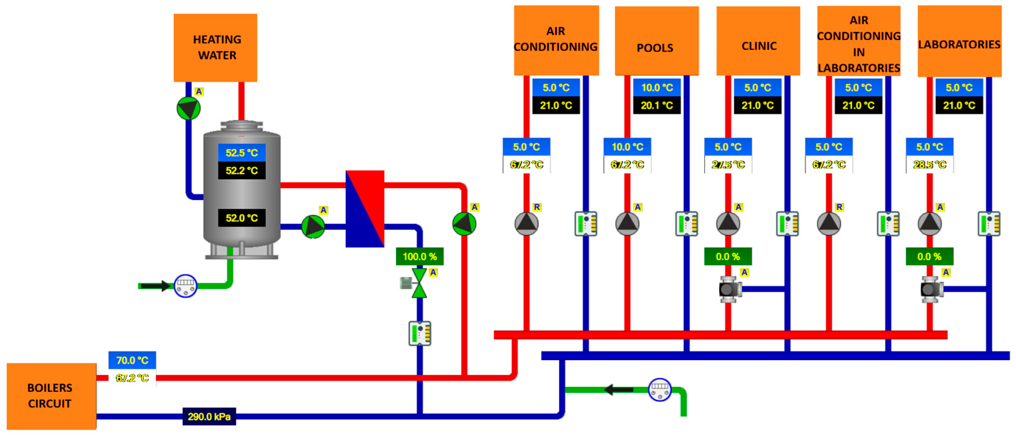
The data were obtained from the facility’s building control system (the scheme is in Figure 1), which continuously monitors alarms, equipment failures, outdoor temperature, and the consumption of all utility media—including gas, water, and electricity. Specifically, the system enables configuration and control of four Danfoss gas boilers, which provide heating and hot water for five distinct building zones (see Figure 2).
To develop a 7-day-ahead gas consumption forecasting model, we selected two key variables from the range of monitored data: outdoor temperature and daily gas consumption. The dataset spans eleven years, from 15 August 2014 to 30 June 2025.
Each gas consumption data point represents the total consumption over a 24 h period for a given day. Correspondingly, the daily temperature value is computed as a weighted average of the temperatures recorded at 07:00, 14:00, and 21:00 on the same day. The total number of days (and therefore data samples) in the time series is 3974, accounting for three leap years and two partial calendar years.
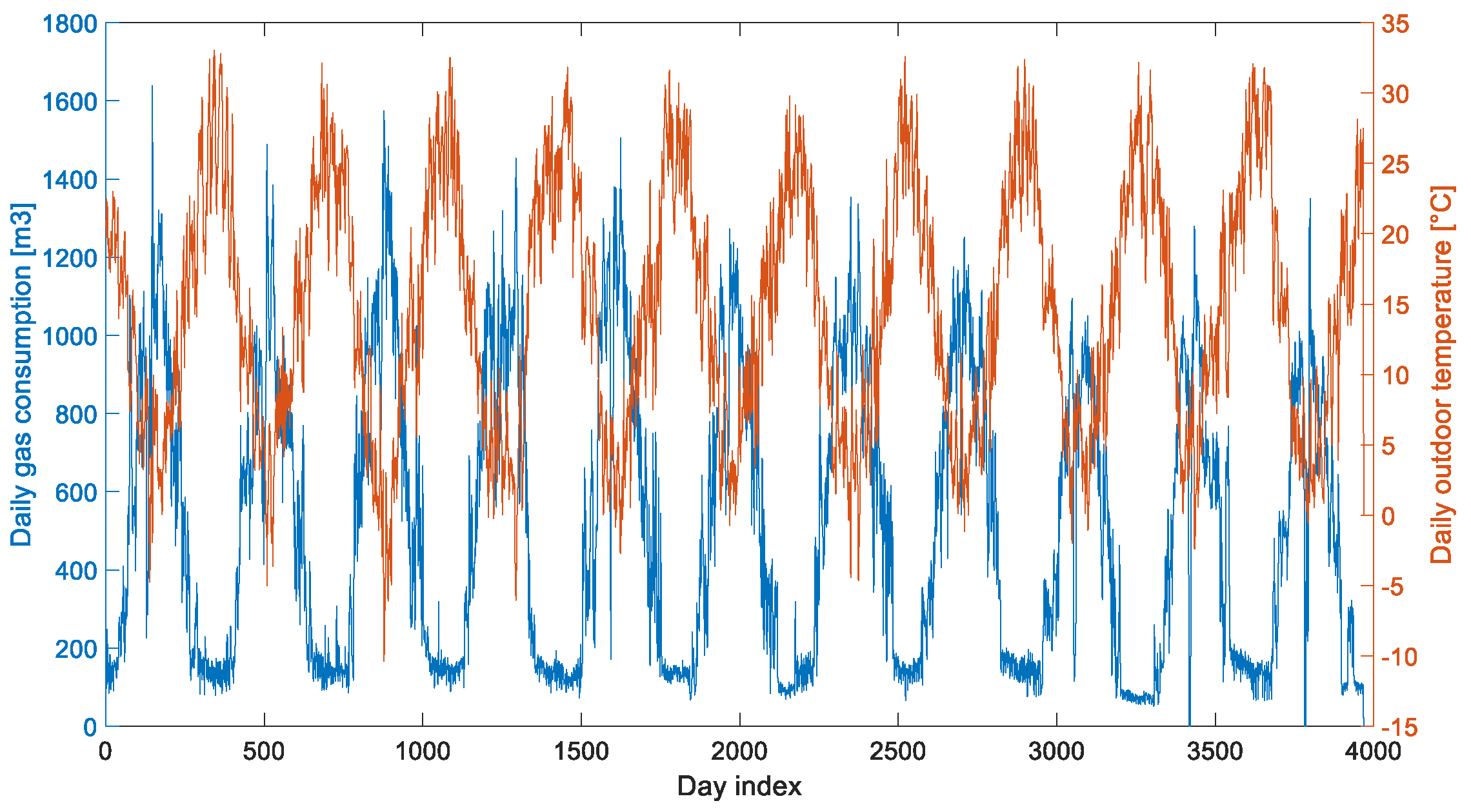
Figure 3 presents the raw gas consumption data. At first glance, certain system outages can be observed, leading to anomalous (outlier) values or missing entries. These cases were identified and, in extreme situations, considered either for exclusion or substitution. Based on the geographical location of the facility, it is possible to distinguish between heating and non-heating periods. Notably, gas consumption never drops to zero, indicating its continued use for water heating even during the summer months. The figure also displays the raw time series data representing outdoor temperature. Given the biannual seasonality and the clear relationship between gas consumption and outdoor temperature—particularly its strong correlation with the heating season—we selected 213 (or 214) heating days from each year for further analysis. Since the monitoring was carried out through a commercial service, the occurrence of missing data was minimised in the interest of service quality. Missing data occurred in 0.25% of cases (5 out of 2130) and were caused by power or internet outages at the time of recording. Outliers were observed even less frequently, primarily due to failures of the monitoring system itself or during repair or replacement of devices, usually outside the heating season. Missing values were imputed using the mean of surrounding observations. The occurrence of 29 February in a leap year was adjusted by omitting this date. The heating season is defined as lasting from 1 October to 30 April, resulting in a total of 2130 data samples across the analysed period.
Additional insights into annual and heating season gas consumption patterns are provided in Table 1 and Figure 4. Due to the data partitioning required for the application of the LSTM model, statistical analysis was performed on only ten heating seasons. According to the values presented in Table 1, the highest average and total gas consumption occurred during the 2016/2017 heating season. This winter period also recorded the lowest average outdoor temperature as well as the lowest absolute temperature. A similar pattern was observed in the 2019/2020 season, which had the lowest average and total gas consumption, coinciding with the highest average and absolute outdoor temperatures recorded to date. In Figure 4, it is also evident that several outliers in daily gas consumption and temperature were identified.
The heating seasons of 2020 and 2021 might have been influenced by the operational changes due to the COVID-19 pandemic; however, the consumption data do not clearly reflect this impact.
For instance, the winter of 2020/2021 shows comparable gas consumption to the 2017/2018 season, where slightly lower outdoor temperatures corresponded to marginally higher consumption. The gas crisis manifested during the winter of 2022/2023, when, at comparable temperature levels, daily gas consumption was reduced to approximately 80% of that in previous years. The 2023/2024 heating season was characterised by above-average temperatures, resulting in consumption levels similar to the previous year but substantially lower than in 2019/2020. And another phenomenon appeared the past heating season: during the holiday period, the boiler rooms were completely shut down.
The objective of this study is to develop a model for forecasting gas consumption up to seven days ahead in monitored facilities. We compare two different methodological approaches.
Due to the strong dependence of gas consumption on outdoor temperature, the linear component related to temperature is removed in both approaches, and subsequent analyses are conducted exclusively on the residuals. Correlation and regression analyses were performed using standard methods, such as those described in [26]. Given the evident temperature dependence, even a simple temperature-based regression model can serve as a baseline for comparison with actual gas consumption.
Initially, a time-independent linear regression model was applied to the gas consumption data to extract residuals. For subsequent time series modelling, ten heating seasons were selected from the available 2343 samples, reserving the 11th season for testing purposes. Consequently, the training dataset comprises 2130 samples of daily gas consumption and corresponding recorded temperatures.
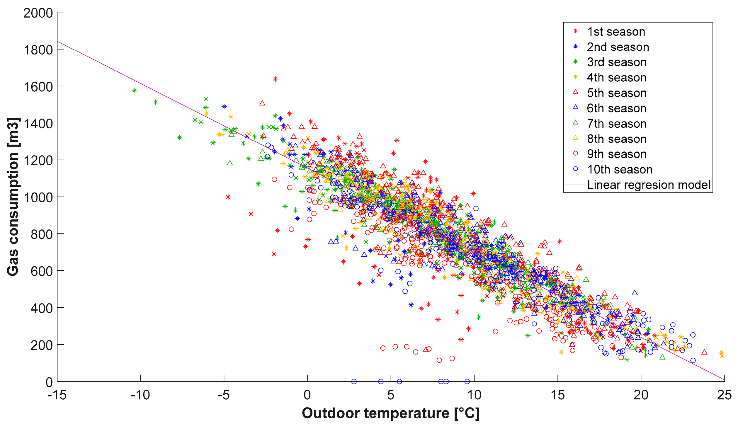
Figure 5 illustrates the linear regression relationship between the daily average outdoor temperature and the daily gas consumption in the studied facility.
This relationship was derived from the data corresponding to ten heating seasons, as shown in Figure 5. A preliminary inspection of the graphs reveals a strong correlation between daily gas consumption and outdoor temperature. Several observations can be made based on this analysis.
Referring to Table 1, the winter of 2016/2017, which experienced low outdoor temperatures, corresponds to data points located to the left of the regression line. The winter of 2018/2019 lies close to the regression line and, despite relatively high average temperatures, exhibited high gas consumption. The 2019/2020 season shows lower consumption values (below the regression curve), which aligns with higher average outdoor temperatures, causing a rightward shift along the line.
Furthermore, the 2020/2021 season closely follows the regression curve, indicating that the impact of the COVID-19 lockdown on gas consumption is not evident in the data. In the last two seasons, 2022/2023 and 2023/2024, zero gas consumption values were recorded during the Christmas holidays.
Linear correlation y = p 1 · x + p 2 with coefficients (with 95% confidence bounds):
p 1 = 45.85     ( 46.83 ,   44.87 )
p 2 = 1155     ( 1145 ,   1165 )
was confirmed by values in Table 2.
By obtaining the LR function, we can also quickly construct a residual graph (see Figure 6), which confirmed our reasoning from Figure 5.

2. Materials and Methods

After removing the linear component, a model for 7-day-ahead prediction of the residuals was created in the next step. From Figure 6, it is evident that no further clear dependencies are identified, and the residuals are influenced by other meteorological factors or by the current gas consumption for water heating.
Therefore, this section will focus on the theoretical aspects of wavelet transform, data series augmentation, and methods for quality evaluation.

2.1. Wavelet Transform

The wavelet transform is a powerful mathematical tool that enables highly precise analysis of signals and images. Unlike the classical Fourier transform, which provides a global frequency analysis, the wavelet transform allows for time-frequency localisation, meaning it provides information not only about which frequencies are present in a signal but also about when and where they occur.
In processing nonlinear, non-stationary, and noise-affected signals (e.g., speech, EEG, images), the classical Fourier transform proves insufficient. The wavelet transform decomposes the signal into functions at various scales and positions, called wavelets.
The following key points should be taken into account when applying this method [27,28,29,30]. A wavelet dictionary is constructed from a mother wavelet ψ of zero average
+ ψ ( t ) d t = 0
Which is dilated with a scale parameter s, and translated by τ :
D = ψ τ , s t = 1 s ψ t τ s s R + 0 , τ R
The continuous wavelet transform of f at any scale s and position τ is the projection of f on the corresponding wavelet atom [27,28,30]:
W   f τ , s = f , ψ τ , s = f t · 1 s ψ t τ s d t ,
In the time-frequency plane, the Heisenberg box (Figure 7) of a wavelet atom ψ τ , s is therefore a rectangle centred at τ ,   η s , with time and frequency widths, respectively, proportional to s and 1/s. When s varies, the time and frequency width of this time-frequency resolution cell changes, but its area remains constant. Large wavelet coefficients correspond to rapid signal changes. High frequencies (small s) provide good time resolution, while low frequencies (large s) provide good frequency resolution. Wavelet bases reveal signal regularity and allow for sparse representation, especially for transients and discontinuities.
As we can see in Figure 7, the mother wavelet is obtained by the multiplication (Figure 7c) of a sine function (Figure 7a) with a window (Figure 7b). Figure 7d Wavelets at three scales resulting from the scaling of the mother wavelet ψ ( t ) . Figure 7e Frequency distribution of the power of wavelets shown in Figure 7e. Figure 7f Heisenberg boxes of the wavelet transform [31].
The discrete wavelet transform (DWT) evaluates the CWT at dyadic scales s = 2 j and translations τ = n 2 j , producing approximation and detail coefficients that can reconstruct the original signal. Haar and Daubechies wavelets are widely used orthonormal bases, with Daubechies db10 employed in this study. The optimal decomposition level is dataset-dependent [32] for our data; level 6 provided the most satisfactory results. The decomposition outcomes are presented in the Section 3. Results and Discussion. The mathematical details and equations of the presented method are in [27,28,29,30,31,32].

2.2. Data Series Augmentation

Since the literature involves several techniques that can potentially be used to augment time series data, it is challenging in practice to investigate all of them. Our objective is to augment the data while preserving the curve’s structural characteristics and its statistical properties. Similar challenges are explored by the authors in [33], where nine effective data augmentation methods are discussed. The following methods are presented and analysed: Horizontal/Vertical Flipping, Time series Combination/Interpolation/ Generation, etc.
The next source is [34], where the authors say that DA techniques are useful for synthetically increasing the number of training samples in a dataset. They used several time series-based DA techniques to artificially generate time series. Namely, GRATIS, MBB, and DBA. The MBB [35] and DBA [36] methods are expected to generate time series from a similar DGP to that of the original series, whereas the GRATIS method generates time series with diverse characteristics from different DGPs, not related to the original dataset. In this context, it would be useful to include a short comparison of MBB with other available techniques, as this strengthens the justification for its selection. While GRATIS offers more diverse but less structurally faithful synthetic series, and DBA aims at averaging multiple series to extract representative patterns, MBB stands out for its ability to preserve temporal dependencies and local correlations. This property makes it particularly suitable for applications where maintaining the statistical resemblance to the original dataset is critical, such as energy consumption modelling. For the reason mentioned above, we prefer the MBB method.
In the following, we have briefly described the method used and explained how we exactly use it in our experiments. MBB (Moving Block Bootstrap) is a method used for data augmentation and the generation of new synthetic samples that remain consistent with the original data. MBB is a resampling technique primarily applied to time series data. It is a variant of the classical bootstrap method that accounts for dependencies between observations—for example, when the data are not independent and identically distributed (i.i.d.), which is typical for time series. MBB is often used in situations where only a limited amount of training data is available and there is a need to increase its diversity or quantity. It can be applied in various domains such as image processing, speech recognition, bioinformatics, or financial modelling.
In our experiment to generate multiple copies of a time series, we first use linear regression wave transform to extract and subsequently remove seasonal and trend components of a time series. Next, the MBB technique is applied to the residuals of the time series, i.e., seasonally and trend-adjusted series, to generate multiple versions of the residual components.
The results of the wavelet transformation, specifically the obtained approximations and details described above, were used to augment the dataset using the MBB method. Since each sample can be reconstructed through summation, we applied moving blocks of approximations and details across different seasons (10 seasons) to generate new data with statistical properties closely resembling those of the original dataset. We chose to vary the approximation component itself, as well as details at levels D5 and D6 (low-frequency details), and D1 and D2 (noise-level details).
Another challenge lies in evaluating the quality of synthetic data and determining whether predictions made using such data can be considered reliable.
The authors of [33] state that, due to the specific nature of the time series domain, there is no single universal metric for evaluating the reliability of algorithms across all their applications. Finding a measure capable of assessing both the quality and diversity of synthetic data remains an open question.
When applying data augmentation (DA) to a dataset, the most common goal is to generate new samples in order to improve the performance of certain models, thereby reducing data imbalance or scarcity. One of the most popular approaches to assess how the addition of new data affects model behaviour is to simply compare the models before and after DA. This makes it possible to evaluate whether each model improves its performance after data augmentation is applied to the input.
This type of evaluation is purely practical and relies on the correlation between a model’s performance and not on the intrinsic quality of the synthetic samples themselves. Most traditional algorithms base their performance assessment on this method, as it provides a direct and straightforward way to evaluate the algorithm.
In [34], the performance of the proposed data augmentation algorithms is assessed using the symmetric mean absolute percentage error (sMAPE) and the mean absolute scaled error (MASE), which are among the most widely adopted evaluation metrics in forecasting tasks. The research involves a comparative analysis of these metrics before and after the application of data augmentation to the dataset, thereby enabling an evaluation of the extent to which model performance improves following the incorporation of additional training data. Similarly, the authors of [37] state: To measure the performance of the proposed framework and benchmarks, they used two metrics commonly found in the forecasting literature, namely the symmetric Mean Absolute Percentage Error (sMAPE) and the Mean Absolute Scaled Error (MASE). In our paper, we have extended the group of metrics with additional ones: the Mean Squared Error (MSE), the Normalised Root Mean Squared Error (NRMSE) or the Normalised Mean Squared Error (nMSE). The metrics are used in the work not only to evaluate the quality of synthetic data but also to assess the quality of the prediction, so we will list them all in a general form:
M A E = 1 n · i = 1 n y i y ^ i
M A P E = 100 % n · i = 1 n y i y ^ i y i
And the second one is normalised errors, such as Mean Absolute Error (nMAE), which is defined as follows:
n M A E = M A E Y ¯ = 1 Y ¯ · n i = 1 n y i y ^ i
n M A E = M A E m a x ( Y ) m i n ( Y )
where y i represents the observation at i, y ^ i   is the generated synthetic/predicted sample, Y ¯ is the mean of the observations at I, and n indicates the number of samples.
Another metric, MSE, is defined as follows:
M S E = 1 n i = 1 n y i y ^ i 2 ,
R M S E = 1 n i = 1 n y i y ^ i 2
where y i represents the observation at time i, y ^ i is the generated synthetic/predicted sample, and n indicates the number of samples. NRMSE is defined as follows:
N R M S E = R M S E Y ¯ = 1 n i = 1 n y i y ^ i 2 Y ¯
N R M S E = R M S E max ( Y ) min Y = 1 n i = 1 n y i y ^ i 2 r a n g e ( Y )
where y i represents the observation at time i, y ^ i is the generated synthetic/predicted sample, and n indicates the number of samples.
And finally, NMSE:
N M S E = i = 1 n y i y ^ t 2 i = 1 n y i Y ¯ i 2 = M S E v a r ( Y )
where y i represents the observation at time i, y ^ i is the generated synthetic/predicted sample, Y ¯ i is the average value of observation, and n indicates the number of samples. In our study, these metrics were used as a qualitative comparison of the effectiveness of the bootstrapping method but also for the prediction performance of the LSTM model.

2.3. Long Short-Term Memory

The Long Short-Term Memory (LSTM) network, proposed by Hochreiter and Schmidhuber (in 1997), is a type of Recurrent Neural Network (RNN) designed to capture both short- and long-term dependencies in sequential data. Unlike traditional RNNs, which struggle with long-term dependencies due to the vanishing gradient problem, LSTMs use a memory cell and gating mechanisms (input, forget, and output gates) to control information flow, enabling selective retention or forgetting of data.
The LSTM cell’s internal state is updated via linear interactions, allowing smooth backpropagation through time and enhanced memory capacity. Commonly used LSTM architectures follow the design by Graves and Schmidhuber (in 2005). Nonlinear transformations (typically hyperbolic tangents) and sigmoids in the gates regulate how inputs, internal states, and outputs are combined. The forward pass equations define the forget gate, candidate state, update gate, cell state, output gate, and final output, using weight matrices for inputs and recurrent connections, bias vectors, and element-wise operations. More details are in the literature [38].
The difference equations that define the forward pass to update the cell state and to compute the output are listed below.
Forget   gate :   σ f t = σ W f x t + R f y t 1 + b f Candidate   state :   h ~ f t = g 1 W h x t + R h y t 1 + b h Update   gate :   σ u t = σ W u x t + R u y t 1 + b u Cell   state :   h t = σ u t h ~ t + σ f t h t 1 Output   gate :   σ o t = σ W o x t + R o y t 1 + b o Output :   y t = σ 0 t g 2 h t
where x[t] is the input vector at time t. Wf, Wh, Wu, and Wo are rectangular weight matrices that are applied to the input of the LSTM cell. Rf, Rh, Ru, and Ro are square matrices that define the weights of the recurrent connections, while bf, bh, bu, and bo are bias vectors. The function σ(·) is a sigmoid,1 while g1(·) and g2(·) are pointwise nonlinear activation functions usually implemented as hyperbolic tangents that squash the values in [−1, 1]. Finally, ⨀ is the entry-wise multiplication between two vectors (Hadamard product).

3. Results and Discussion

3.1. Wavelet Transform of Data

In this section, the methods described above and the proposed model are summarised. First, the wavelet transform, introduced in Section 2.1, was employed to generate synthetic data by varying groups of detail coefficients. With the aim of improving the training quality of the LSTM method in future work, we assumed that an increased number of samples would lead to predictions with lower error. We chose to use the wavelet transform for synthetic data generation because we wanted to create a set of synthetic data that approximately matches the shape characteristics of the real data curves. Since wavelet decomposition represents the original signal as the sum of approximations and details, this method fully preserves the mean as a statistical indicator. Naturally, the variance differs (Figure 8).
When reconstructing the signal by summing wavelets, it was necessary to carefully select the decomposition level and decide to which level it is appropriate to mix details—whether to start from D1, D2 or from D5, D6—i.e., which level we consider to represent meaningful seasonality and which corresponds to “white noise.”
Figure 9 shows the wavelet decomposition of several randomly selected seasons, for example: (a) 2014/2015, (b) 2019/2020, (c) 2020/2021 (due to COVID-19), and (d) 2023/2024 (as the global situation significantly affects commodity prices on the world market).
Each heating season exhibits certain “seasonalities.” In the 2022/2023 heating season, the approximation lies within the range of negative values, which may indicate a significant decrease in gas consumption compared to the regression model calculated from all heating seasons (see Figure 5). This could be attributed to energy-saving measures in response to rising gas prices on global markets. This assertion is further supported by the statistical comparison of total consumption and average outdoor temperature shown in Table 1.
It is assumed that around the 85th to 90th day of the season (counting from October 1st), there is a significant reduction in the operation of the facility due to the Christmas holidays. This is subsequently followed by a peak around the 120th to 130th day, which corresponds to the coldest period of the year in these latitudes (January–February).
Detail 2 contains approximately 30 peaks, which correspond to weekly cycles given by 213/7. Detail 1 can be regarded as white noise, representing random phenomena such as increases or decreases due to varying weather conditions or changing demands for hot water consumption, among others.
Critically speaking, the preservation of trends and variations in the wavelet details indicates more than merely the ability to capture seasonality—it also demonstrates that the decomposition can distinguish between high-frequency fluctuations and deeper seasonal trends. This capability is crucial for identifying extreme peaks and unexpected consumption deviations that may be obscured or distorted by noise in traditional methods. The observed shifts in the approximation graphs further suggest that consumption dynamics vary across different seasons, highlighting the risk of overestimating the generalizability of models trained solely on historical data without synthetic augmentation. In this way, wavelet decomposition provides a robust and critically relevant tool for supplementing limited datasets while maintaining the accuracy necessary for reliable predictions and the identification of unforeseen energy fluctuations.

3.2. Performance of Data Augmentation and Quality Control

As mentioned above, the wavelet decomposition to generate synthetic data is used. The number of real samples is 213 samples per season × 10 seasons = 2130 samples. By varying details at two decomposition levels, we obtained 2130 × 10 × 10 samples, i.e., 213,000 synthetic samples (including the real samples). These samples are used to train the LSTM network. For testing, real values from the 11th season, i.e., 177 samples available as of 31 March 2025, were used.
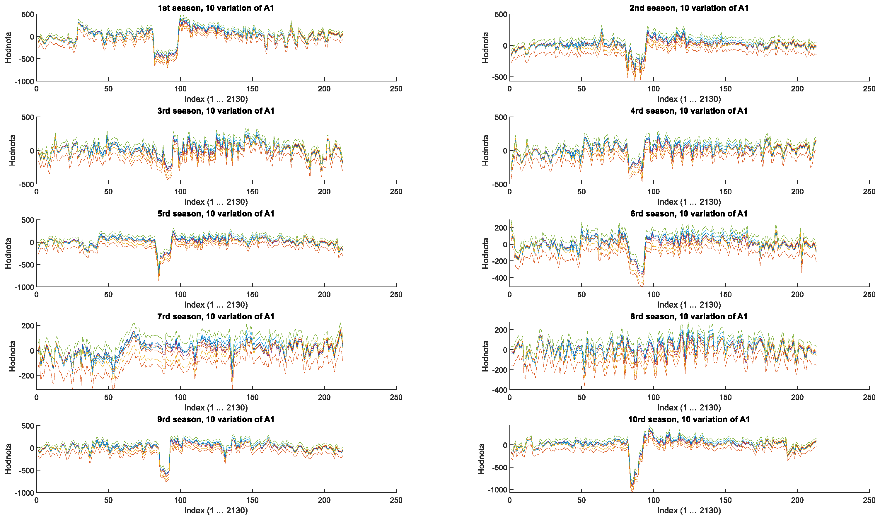
For illustrative purposes, the following figures show 100 mutations of detail levels D1 and D2 (respectively, A1) for each of the 10 seasons. For better readability, Figure 10 displays 10 versions of seasons 1–10 consecutively. In contrast, Figure 11 shows only 10 versions of seasons 1–10. It can be observed that changes in approximation shift the graphs along the y-axis because the approximation in the 10th season was significantly lower. At the same time, it is evident that the synthetic signals preserve the trend of the real signals. Given the matching statistical parameters, this suggests that the synthetic data are suitable for training the network.
Subsequently, the quality of the synthetic data was directly compared. Two metrics, comparing nMAE and NRMSE while varying D1D2, and D5D6, were used in Table 3 and Table 4, both metrics calculated according to the formulas presented in Section 2.2 above as (Equations (6a) and (8b)) as differences between actual and synthetic data. For better illustration, the same seasons as in Figure 9 are chosen.
For Equations (6a) and (8b), the synthetic residuals were converted back to actual values of gas consumption using the coefficients of linear regression, as we aimed to avoid issues with negative or near-zero values. For both metrics in Figure 12 and Figure 13, it is evident that throughout the entire year, the error between the real data and the D1D2 variations (solid line) is higher than the error between the real data and the D5D6 variations (dashed line), with a few exceptions such as January 2015 (season 1) and December 2020 (season 7) observed with both metrics. The results of nMAE and NRMSE are given in Table 3 and Table 4.
If variations of another wavelet level were to be added, the number of samples would be 213,000 × 10 = 2,130,000, which would no longer qualitatively improve the training and would additionally impose a significant burden on hardware requirements and slow down the computation.
According to the results achieved in this chapter, we can conclude that the proposed procedure is suitable for generating synthetic data. It remains a matter of consideration which wavelet components to vary to obtain new datasets. When varying details D1D2, the average nMAE value is 8.5% and the NRMSE value is 12.6%. When varying details D5D6, the average nMAE value is 6.4% and the NRMSE value is 9.9%. From this perspective, generating synthetic data by varying D5D6 appears to be the more suitable approach.
Despite the clear advantages of generating synthetic data via wavelet decomposition, the method also has certain limitations. First, it is sensitive to the choice of decomposition levels—improper selection can lead to excessive amplification of noise or, conversely, to the attenuation of significant fluctuations. Second, the exponential increase in the number of samples when adding additional levels can quickly exceed computational and memory capacities, limiting the scalability of the method for very large datasets. Third, wavelet decomposition assumes that historical consumption patterns and their variations are representative of future periods; unexpected events or structural changes in consumption may cause the synthetic data to fail in accurately reflecting reality. These factors must be taken into account when applying the method to larger datasets or when planning long-term predictions.
Overall, wavelet-based synthetic data generation appears to be a robust tool for supplementing limited datasets while maintaining the accuracy required for reliable predictions and the identification of unforeseen energy consumption fluctuations.

3.3. Use of Long Short-Time Method

Let us summarise the results obtained so far. We subtracted the regression component reflecting the dependency on the outside temperature from the actual daily gas consumption values. This yielded a time series of residuals, which we intend to use for training an LSTM network.
  • The residuals were obtained by subtracting a linear regression model from the original data: r e z = d a t a L R = d a t a ( A T e m p e r a t u r e + B ) .
  • These residuals were subsequently normalised using the standard approach: d a t a n o r m = d a t a d a t a p r i e m d a t a o d c h .
  • And finally, normalised data were split into training and validation datasets in a 90:10 ratio.
In the following, two approaches are compared. First, using the time series data augmentation methodology introduced in Section 3.2, we generated a set of synthetic data to improve training quality. Based on the analysis of our problem, we selected a wavelet decomposition into six detail components, which we consider sufficient. The input to the model consists of the normalised residuals, while the output is the predicted normalised residual value for a 7-day horizon.
The same wavelet decomposition was employed in the second case, but this time the model was trained on each wavelet component separately. In this case, the input is the respective detail (wavelet component) of the normalised residuals, and the output is the predicted value of that same detail component over a 7-day forecast horizon.
These two approaches are subsequently compared using data from Season 11. The prediction errors are evaluated according to the criteria specified in Section 2.3.

3.3.1. Use of LSTM Methods with Synthetic Data

We begin the training process using synthetic data generated by varying the detail components at level A1. According to Figure 11 presented above, the generated synthetic data appear to be “shifted downward” relative to the real data.
The following Figure 14 presents the training results obtained on 21,300 samples from Seasons 1 to 10, including a comparison between the residuals and their predicted values (in normalised form), followed by a comparison between the actual and predicted gas consumption over 177 samples from Season 11. In this case, as well as in all subsequent experiments, the following training parameters were used: Method: SGDM, MaxEpochs: 100, InitialLearnRate: 0.05, LearnRateDropFactor: 0.2. The quality parameters, calculated according to the Formulas (14b) and (16a) defined above, nMAE is 0.184, and the NRMSE is 0.159.
Similarly, we conduct training using synthetic data generated by varying the detail components at levels D1 and D2. The following Figure 15 presents the training results obtained on 213,000 samples, including a comparison between the normalised residuals and their predicted values, followed by a comparison between the actual and predicted gas consumption of Season 11. The resulting error metrics are: nMAE = 0.171, NRMSE = 0.148.
Next, variations to the detail components at levels D5 and D6 to obtain synthetic data were applied. The prediction of the 11th season is shown in Figure 16. The results of this training yield the following error metrics: nMAE = 0.189, NRMSE = 0.156.
Finally, training without the use of synthetic data was performed The results (Figure 17) are highly comparable to those obtained with synthetic data augmentation, nMAE = 0.178 and NRMSE = 0.154.
The results of this Section 3.3.1 are summarised in the following overview Table 5. It must be emphasised that the training using synthetic data generated by varying details D1 and D2 yielded the lowest values across all evaluation metrics: nMAE and NRMSE. Therefore, this particular training configuration will be used as the reference in subsequent comparisons.
Training using the LSTM method reveals certain differences across configurations; however, the results are largely comparable, particularly during stable (typical) operating periods. The predictions for Season 11 achieved the lowest error values when the model was trained using synthetic data generated by varying the D1 and D2 wavelet components.
In contrast, during periods of significant temperature anomalies—when the operational environment deviated from standard behaviour (e.g., sudden changes, heating system shutdowns, or sharp temperature drops)—the best predictive performance was observed in the model trained exclusively on real data, without synthetic augmentation.
Based on these findings, it can be concluded that the use of synthetic data did not deliver the expected improvement in forecasting accuracy. In some cases, training without synthetic data even resulted in better evaluation metrics while also significantly reducing computational time and complexity.
Figure 18a presents a comparison of predicted gas consumption using various methods against the actual consumption. Figure 18b provides a detailed view of the predictions during a stable operational period (i.e., typical conditions).

3.3.2. Use of LSTM for Training of Waves

Due to the high error rates observed with the initial approach (as summarised in Table 5, including metrics such as MAE and NRMSE), a second training strategy was adopted. In this method, wavelet decomposition was utilised, and prediction models for each wavelet component were independently trained. After obtaining the forecasts for all components, the final gas consumption for Season 11 was reconstructed by summing the predicted components, reversing the normalisation, and adding back the linear regression component (Figure 19).
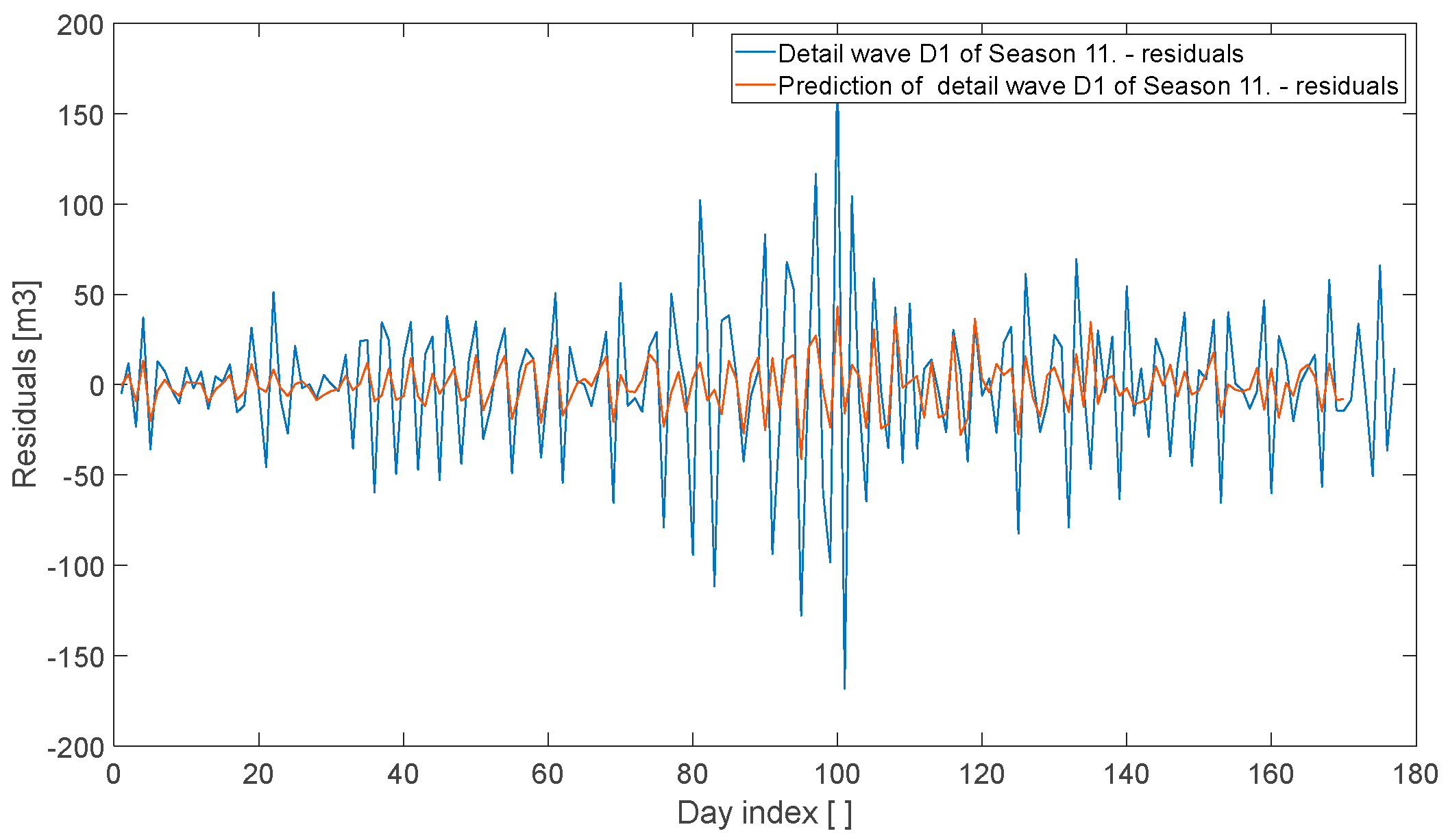
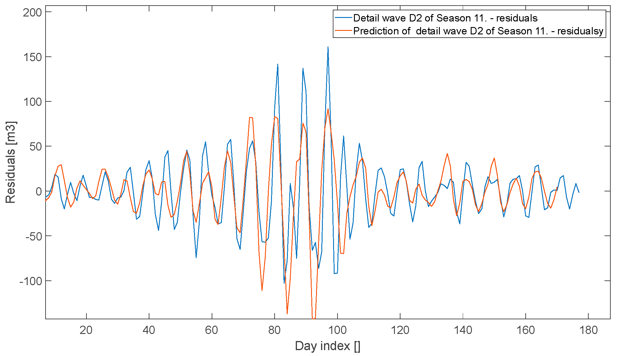
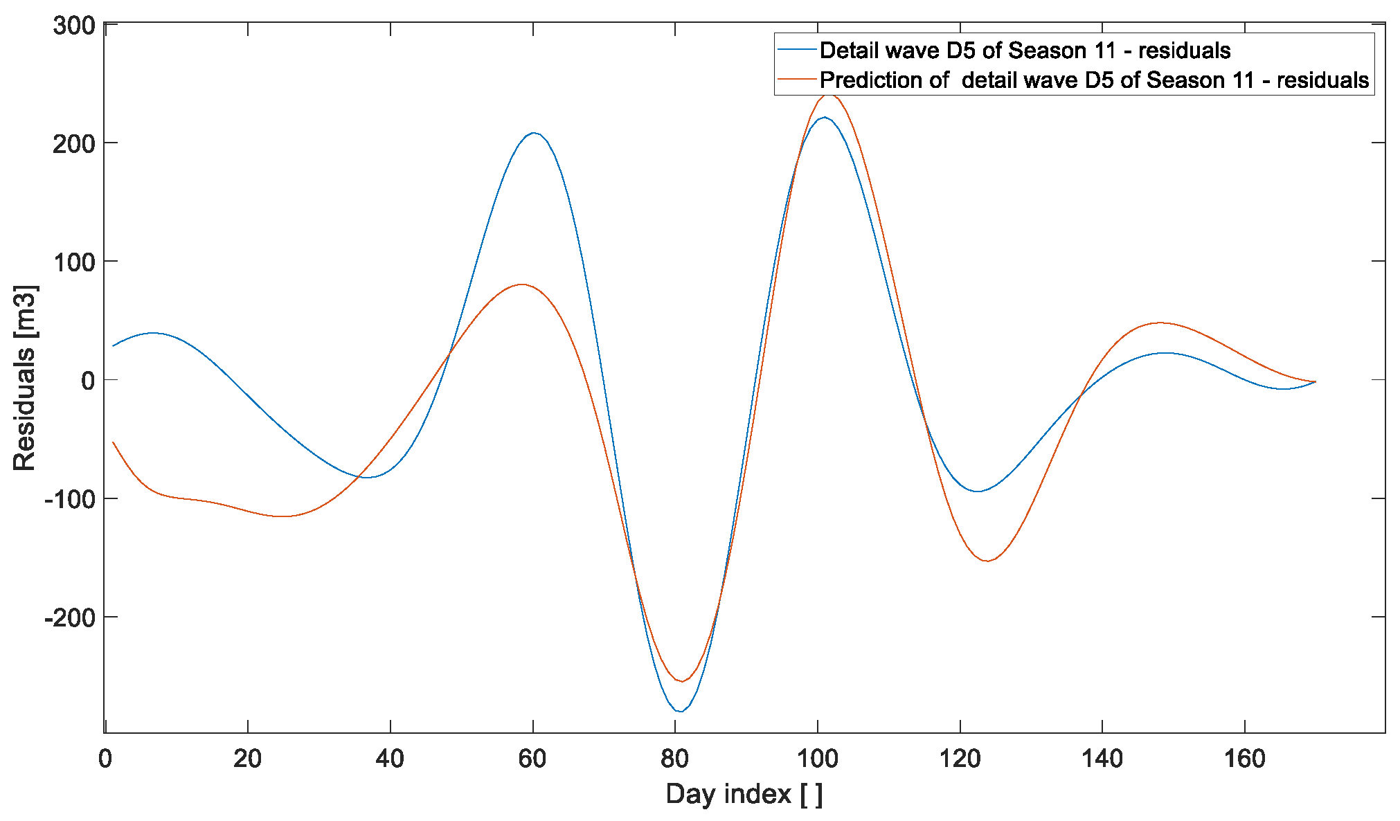
In general, training the approximation component and the coarser detail levels proved to be relatively straightforward. The training parameters applied to these components were: Method: SGDM, MaxEpochs: 100, InitialLearnRate: 0.05, LearnRateDropFactor: 0.2. However, training the finest-scale components, D1 and D2—which are typically dominated by noise—was notably more challenging. To address convergence issues, we modified both the network architecture and training options, using the following updated parameters: Method: Adam, MaxEpochs: 200, InitialLearnRate: 0.005, LearnRateDropFactor: 0.2. Even with these adjustments, the prediction results for D1 and D2 remained inferior compared to those for smoother components such as A1, D5, and D6.
Let us begin by presenting the training of the approximation wavelet component and its prediction for Season 11, shown in Figure 20. Figure 21, Figure 22, Figure 23, Figure 24, Figure 25 and Figure 26 display the prediction results for the detailed components D1 through D6 for the same season.
To summarise Section 3.3.2, we can compare the actual daily gas consumption with the predicted consumption obtained through training on individual wavelet components (Figure 27). The predicted values were derived through the following steps:
  • Summation of the predicted wavelet components.
  • Denormalisation of the resulting signal.
  • Addition of the linear regression component.
This approach proves effective in capturing both typical operational periods and significant anomalies, such as the Christmas week. Moreover, it achieves a 66.5% reduction in prediction error, with nMAE = 0.0571, and NRMSE = 0.0780, highlighting its improved accuracy and robustness over previously tested methods.
The second methodology offers a more efficient solution, as it involves training on only 2130 samples corresponding to the relevant wavelet details extracted from 10 seasons. Despite the significantly reduced dataset size, this approach achieves 66.5% lower error rates compared to the method based on synthetic data augmentation. This demonstrates not only its computational efficiency but also its superior predictive accuracy. For both models discussed in Section 3.3, it must be acknowledged that a model trained on data from a single building may not be directly applicable to other buildings with different structures, heating systems, or consumption profiles. Variations in gas consumption are often specific to a particular building, seasonal habits, or local climatic conditions. Therefore, the predictive model always requires adjustments or supplementary local data to maintain forecasting accuracy in a new context. Table 6 summarises the computational cost for both methods used.

3.4. Prediction of Daily Gas Consumption Based on the Predicted Temperature

The results obtained in Section 3.3.2—based on the wavelet decomposition training (second methodology)—will be further utilised to generate 7-day gas consumption forecasts using 7-day temperature forecasts for the corresponding region. These temperature forecasts pertain to the 11th heating season (2024–2025), enabling a direct comparison between:
  • Actual gas consumption.
  • Predicted consumption based on actual temperatures.
  • Predicted consumption based on forecasted temperatures.
The temperature forecasts were obtained from the Norwegian Meteorological Service (yr.no) through its publicly available API, which delivers data in JSON format. For this work, we employ forecasts generated by the ECMWF (European Centre for Medium-Range Weather Forecasts), a highly regarded forecasting system widely used by numerous national meteorological agencies—including the Slovak Hydrometeorological Institute (SHMÚ), where it appears as part of the IFS (Integrated Forecasting System) output.
We conducted a detailed evaluation of the 7-day forecast accuracy of the ECMWF model. Key characteristics of the model include:
  • ECMWF: European Centre for Medium-Range Weather Forecasts.
  • Operates the IFS global weather prediction model.
  • Provides forecasts up to 10–15 days in advance, with a 7-day horizon considered its optimal range.
  • Updated twice daily (00:00 and 12:00 UTC).
The Norwegian temperature forecast model is widely recognised as one of the most accurate, particularly for Northern and Central Europe. It is generally more reliable for our region than the American GFS model, with reported 7-day forecast reliability between 85 and 88% and a mean absolute error (MAE) of approximately 1.8 °C.
We recorded temperature forecasts starting from the 2023–2024 heating season, specifically at 6:00, 12:00, and 18:00, based on available data. As mentioned previously, actual temperature measurements were taken three times daily using a sensor installed in the monitored facility. To compute the daily average outdoor temperature, we followed the methodology specified in the [39], which defines the weighted arithmetic mean of temperatures measured in the shade at 7:00, 14:00, and 21:00, assigning a double weight to the 21:00 value.
Based on our recorded values, we obtained a mean absolute error (MAE) of 2.48 °C. This deviation exceeds the expected 1.8 °C stated for the ECMWF model and may be attributed to data incompatibilities or the specific location and conditions of the temperature sensor.
The graph (Figure 28) presents a comparison between the 7-day temperature forecast and the actual measured temperatures, starting from the beginning of the heating season on 1 October 2024. Despite the occurrence of a higher Mean Absolute Error (MAE), the forecasted trend remains largely comparable to the actual temperature progression, indicating that the model provides sufficient accuracy for the purposes of gas consumption prediction.
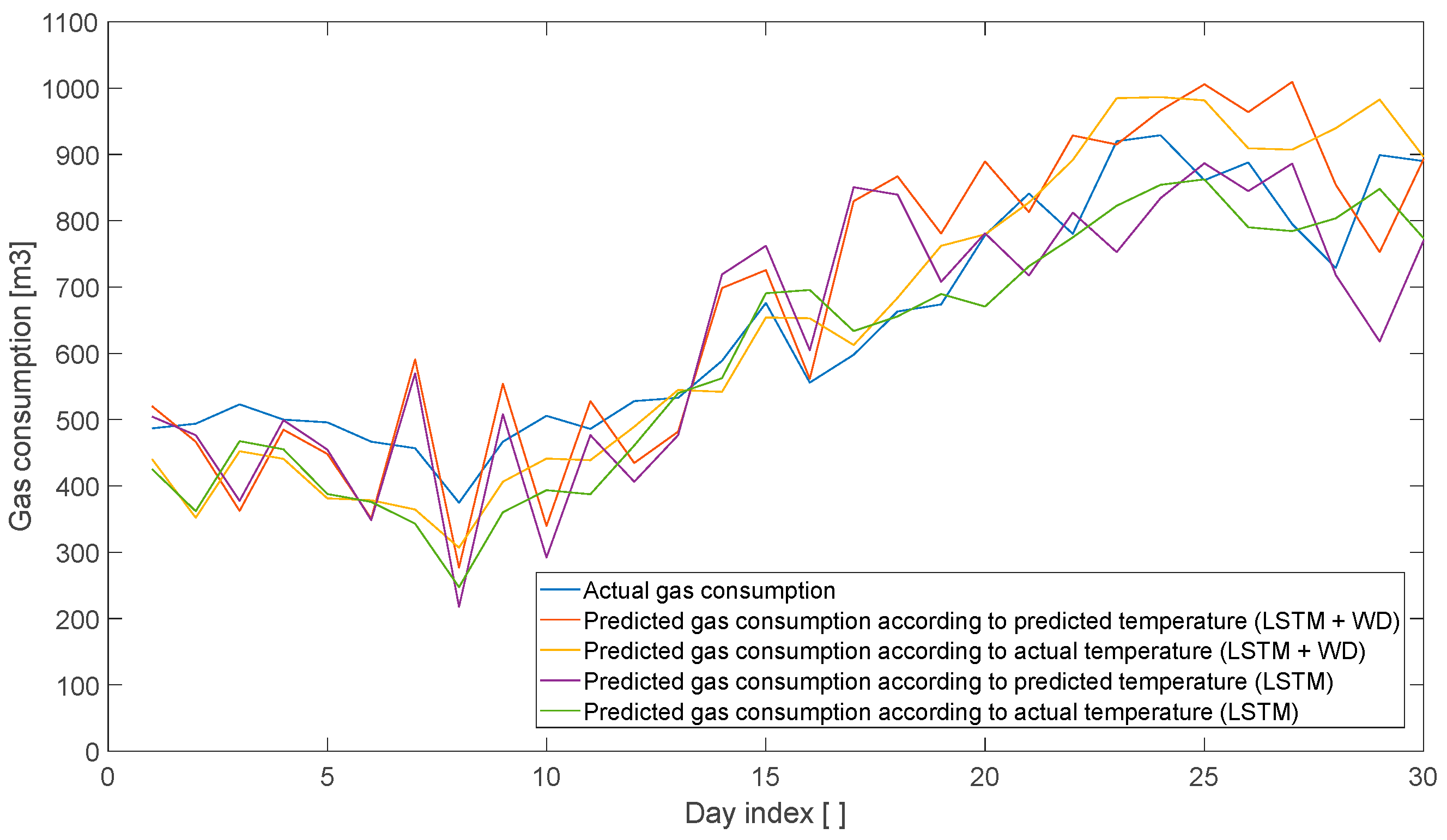
For the predictive model, we selected 30 samples that fall within the 1.8 °C error limit for ECMWF. The comparison focuses on the 7-day gas consumption forecast based on the 7-day temperature forecast, the 7-day gas consumption forecast based on the 7-day actual temperature and actual daily gas consumption. Both methods, LSTM without synthetic data and LSTM with wavelet decomposition training, can be seen in Figure 29.
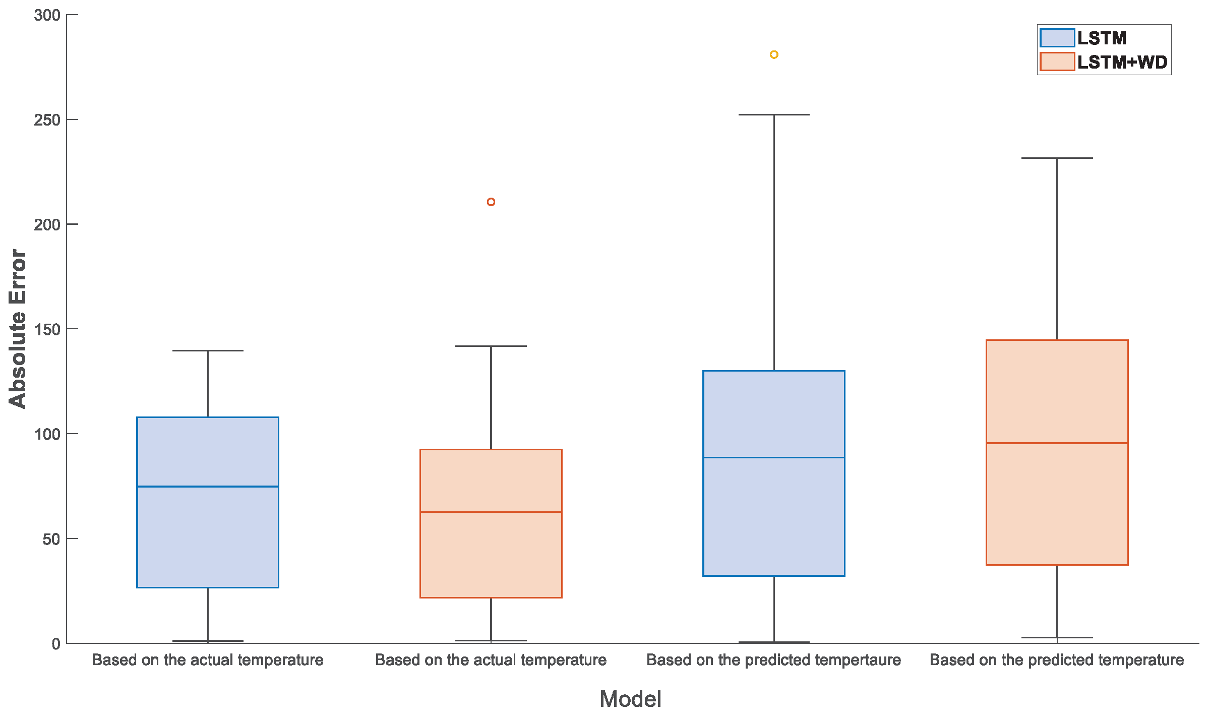
The MAE between the actual gas consumption and the predicted consumption based on the forecasted temperature is 0.138.

3.5. Summary of Results

This article discusses the prediction of a 7-day daily natural gas consumption forecast for a selected facility located in the Slovak Republic. Among the meteorological variables, we employed historical records of actual daily temperatures measured directly at the site. As will be demonstrated in subsequent sections, we also developed forecasts of natural gas consumption based on predicted daily temperatures. For this purpose, we utilised archived forecasts from the ECMWF model available via the yr.no platform. The operational characteristics and statistical indicators of the selected facility are presented in Table 1 and Figure 3 and Figure 4. The first ten heating seasons were utilised for training the neural network. The winter operation period comprised 213 × 10 observations of daily gas consumption, along with the corresponding 213 × 10 samples of average daily temperature.
Given the evident dependency of gas consumption on outdoor temperature, the initial step involved the development of a linear regression model. This model was employed to remove the linear component from the dataset, allowing the subsequent modelling to focus solely on the prediction of residuals as a time series (see Figure 5).
To summarise the achieved results. A 7-day gas consumption forecast was generated using the Long Short-Term Memory (LSTM) method. Within the scope of this study, the following models were compared:
  • To enhance the quality of the prediction, we expanded the dataset with synthetic data. These were generated using Wavelet Transform (see Figure 8), by varying approximation components and selected detail components (see Figure 9 and Figure 10). The quality of the augmented dataset was evaluated using normalised Mean Absolute Error (nMAE) and normalised Root Mean Square Error (NRMSE). Training results and comparisons with actual data from the 11th heating season are presented in Figure 14, Figure 15, Figure 16 and Figure 17, with nMAE and NRMSE values summarised in Table 5. However, this approach did not yield the expected improvement. The most promising results were achieved either by models trained on real data alone (computationally less demanding) or by using data with detailed components D1 and D2, varied only within the noise level. As demonstrated in Figure 18, a major limitation of this method is its inability to adequately capture consumption behaviour during operational interruptions caused by holidays.
  • The second approach excluded synthetic data entirely. The Wavelet Transform was applied and proposed to improve prediction accuracy by forecasting each wavelet component individually (see Figure 20, Figure 21, Figure 22, Figure 23, Figure 24, Figure 25 and Figure 26). The residual prediction was obtained by summing the predicted wavelet components, and the final gas consumption forecast was reconstructed by adding the previously separated linear component (temperature-dependent). The results, presented in Figure 27, show a 66% improvement in both nMAE and NRMSE compared to the previous approach. This methodology proved significantly more robust in handling operational downtimes during the winter holiday period. Specifically, we achieved nMAE = 5.71% and NRMSE = 7.80%.
  • In the third stage, we employed the best-performing model from Approach 1 and the best-performing model from Approach 2 to generate a 7-day forecast of gas consumption based on 7-day temperature forecasts. The results were then compared to those of models that relied on actual observed temperature and gas consumption data (see Figure 29).
Finally, in all cases, the MAEs (Mean Absolute Errors) were compared. As can be seen in Figure 30, the results of the LSTM method, where wavelet decomposition is used, show the smallest median, quartile and outliers. The use of the predicted temperature slightly worsened the results for both methods. (Figure 31).

4. Conclusions

The issue of energy consumption forecasting is becoming increasingly prominent due to escalating global conflicts, which often take place in regions rich in natural resources such as oil, natural gas, and coal. These conflicts have a direct impact on the stability of energy markets and significantly affect the availability and price of energy on global markets. As a result, there is growing pressure on countries, municipalities, and individual organisations to optimise energy consumption and ensure its efficient use.
This is particularly important in regions where climatic and geographical conditions—especially latitude—significantly influence energy demands for heating or cooling buildings. In such contexts, energy consumption forecasting becomes an essential tool for planning and managing energy resources. Accurate forecasts not only help ensure uninterrupted supply but also minimise surplus reserves, reduce economic costs, and limit environmental impacts such as excessive greenhouse gas emissions.
Given the continuously rising demand for energy, changes in the structure of production and consumption, and increasing sustainability requirements, research in the field of energy consumption prediction is rapidly evolving. A large body of available scientific literature and academic research confirms the importance and relevance of this topic. Approaches based on artificial intelligence, machine learning, or hybrid models that combine multiple techniques are increasingly applied to enhance the accuracy and reliability of predictions.
From this perspective, energy consumption forecasting can be seen not only as a key tool for operational efficiency but also as a critical component of the global effort to reduce environmental burdens and achieve climate neutrality targets.
With the development of artificial intelligence methods and the growth of computational capabilities, new opportunities are emerging for applying these advanced technologies in the field of energy consumption forecasting. Traditional statistical methods, such as linear regression or ARIMA models, often reach their limits when dealing with the nonlinear and highly variable data typical of energy systems influenced by many external factors—from meteorological conditions to consumer behaviour.
Modern artificial intelligence methods—especially machine learning and deep learning—can overcome these limitations. Models such as neural networks, support vector machines (SVMs), random forests, and particularly recurrent neural networks (RNNs) and their variants like LSTM (Long Short-Term Memory) are increasingly used for modelling and forecasting energy consumption time series. These models are capable of capturing complex relationships and dependencies in the data, including seasonality, trends, and sudden fluctuations.
An interesting approach also lies in combining classical analytical tools with machine learning. For example, the use of wavelet decomposition allows the original time series to be broken down into several frequency components, thereby removing noise and highlighting important patterns in the data. Training a predictive model—such as an LSTM network—on these cleaned and processed components can significantly improve forecasting accuracy.
Moreover, with the increasing availability of historical energy consumption data and related datasets (e.g., meteorological data, energy prices, demographic factors), conditions are emerging for the development of robust models that can adapt to changing conditions in real time. These intelligent systems have the potential not only to forecast consumption with high accuracy but also to support decision-making in energy management, production planning, distribution, and cost optimisation.
The direction of research clearly indicates that the integration of artificial intelligence into the energy sector will play an increasingly significant role in the coming years. On one hand, research can focus on forecasting the daily energy consumption of individual buildings, enabling operators to anticipate extreme peaks and ensure adherence to daily or monthly consumption limits. Exceeding these thresholds may result in increased operational costs, penalties, or adjustments to pricing tariffs. On the other hand, the joint analysis of extensive building datasets using predictive machine learning models allows for the precise identification of the parameters that exert the greatest influence on energy consumption. This approach provides a foundation for further research aimed at identifying key parameters and clustering building typologies, thereby mitigating cost escalation and supporting the optimisation of building operational efficiency [40].
The result may be not only greater operational efficiency but also a reduction in environmental impact and an increase in energy security—key priorities in the context of today’s global challenges.

Author Contributions

Conceptualization, A.H. and J.M.; methodology, A.H.; software, J.M.; validation, B.P. and P.P.; formal analysis, J.M.; investigation, J.M., P.P. and A.H.; resources, P.P. and B.P.; data curation, B.P.; writing—original draft preparation, J.M.; writing—review and editing, A.H., B.P. and P.P.; visualisation, J.M.; supervision, A.H.; project administration, A.H. and B.P.; funding acquisition, A.H. and B.P. All authors have read and agreed to the published version of the manuscript.

Funding

This research was funded by the Scientific Grant Agency of the Ministry of Education, Research, Development and Youth of the Slovak Republic and the Slovak Academy of Sciences under the project VEGA 1/0704/22; and by the EU NextGenerationEU through the Recovery and Resilience Plan for Slovakia under the project No. 09I03-03-V03-00075. This work was also supported by Early Stage Grant No. 48/2024/ESGTUKE within the EU NextGenerationEU through the Recovery and Resilience Plan for Slovakia under the project No. 09I03-03-V05-00015.

Institutional Review Board Statement

Not applicable.

Informed Consent Statement

Not applicable.

Data Availability Statement

Dataset is available on request from the authors.

Acknowledgments

The authors have reviewed and edited the output and take full responsibility for the content of this publication.

Conflicts of Interest

The authors declare no conflicts of interest.

References

  1. Mahjoub, S.; Chrifi-Alaoui, L.; Marhic, B.; Delahoche, L. Predicting Energy Consumption Using LSTM, Multi-Layer GRU and Drop-GRU Neural Networks. Sensors 2022, 22, 4062. [Google Scholar] [CrossRef] [PubMed]
  2. Noaman, S.A.; Sahmed Ahmed, A.M.; Salman, A.D. A Prediction Model of Power Consumption in Smart City Using Hybrid Deep Learning Algorithm. Int. J. Inform. Vis. 2023, 7, 2436–2444. [Google Scholar]
  3. Caicedo-Vivas, J.S.; Alfonso-Morales, W. Short-Term Load Forecasting Using an LSTM Neural Network for a Grid Operator. Energies 2023, 16, 7878. [Google Scholar] [CrossRef]
  4. Chévez, P.; Martini, I. Applying neural networks for short and long-term hourly electricity consumption forecasting in universities: A simultaneous approach for energy management. J. Build. Eng. 2024, 97, 110612. [Google Scholar] [CrossRef]
  5. Liu, J.; Wang, S.; Wei, N.; Chen, X.; Xie, H.; Wang, J. Natural gas consumption forecasting: A discussion on forecasting history and future challenges. J. Nat. Gas Sci. Eng. 2021, 90, 103930. [Google Scholar] [CrossRef]
  6. Tamba, J.G.; Essiane, S.N.; Sapnken, E.F.; Koffi, F.D.; Nsouandélé, J.L.; Soldo, B.; Njomo, D. Forecasting Natural Gas: A Literature Survey. Int. J. Energy Econ. Policy 2018, 8, 216–249. [Google Scholar]
  7. Liu, J.; Wang, S.; Wei, N.; Yang, Y.; Lv, Y.; Wang, X.; Zeng, F. An Enhancement Method Based on Long Short-Term Memory Neural Network for Short-Term Natural Gas Consumption Forecasting. Energies 2023, 16, 1295. [Google Scholar] [CrossRef]
  8. Ghasemi, F.; Mehridehnavi, A.; Fassihi, A.; Pérez-Sánchez, H. Deep neural network in QSAR studies using deep belief network. Appl. Soft Comput. 2018, 62, 251–258. [Google Scholar] [CrossRef]
  9. Šebalj, D.; Mesaric, J.; Davor, D. Analysis of Methods and Techniques for Prediction of Natural Gas Consumption: A Literature Review. J. Inf. Organ Sci 2019, 43, 99–117. [Google Scholar] [CrossRef]
  10. Paravantis, J.A.; Malefaki, S.; Nikolakopoulos, P.; Romeos, A.; Giannadakis, A.; Giannakopoulos, E.; Mihalakakou, G.; Souliotis, M. Statistical and machine learning approaches for energy efficient buildings. Energ. Build. 2025, 330, 115309. [Google Scholar] [CrossRef]
  11. Smajla, I.; Vulin, D.; Sedlar, D.K. Short-term forecasting of natural gas consumption by determining the statistical distribution of consumption data. Energy Rep. 2023, 10, 2352–2360. [Google Scholar] [CrossRef]
  12. Smalja, I.; Sedlar, D.K.; Vulin, D.; Jukić, L. Influence of smart meters on the accuracy of methods for forecasting. Energy Rep. 2021, 7, 8287–8297. [Google Scholar] [CrossRef]
  13. Deb, C.; Zhang, F.; Yang, J.; Lee, S.E.; Shah, K.W. A review on time series forecasting techniques for building energy consumption. Renew. Sustain. Energy Rev. 2017, 74, 902–924. [Google Scholar] [CrossRef]
  14. Manigandan, P.; Alam, M.S.; Alharthi, M.; Khan, U.; Alagirisamy, K.; Pachiyappan, D.; Rehman, A. Forecasting Natural Gas Production and Consumption in United States-Evidence from SARIMA and SARIMAX Models. Energies 2021, 14, 6021. [Google Scholar] [CrossRef]
  15. Rehman, A.; Zhu, J.-J.; Segovia, J.; Anderson, P.R. Assessment of deep learning and classical statistical methods on forecasting hourly natural gas demand at multiple sites in Spain. Energy 2022, 244, 122562. [Google Scholar] [CrossRef]
  16. Wang, H.; Gao, X.; Zhang, Y.; Yang, Y. Natural Gas Consumption Forecasting Model Based on Feature Optimization and Incremental Long Short-Term Memory. Sensors 2025, 25, 2079. [Google Scholar] [CrossRef]
  17. Peng, S.; Chen, R.; Yu, B.; Xiang, M.; Lin, X.; Liu, E. Daily natural gas load forecasting based on the combination of long short term memory, local mean decomposition, and wavelet threshold denoising algorithm. J. Nat. Gas Sci. Eng. 2021, 95, 104175. [Google Scholar] [CrossRef]
  18. Chen, Y.; Xu, X.; Koch, T. Day-ahead high-resolution forecasting of natural gas demand and supply in Germany with a hybrid model. Appl. Energ. 2020, 262, 114486. [Google Scholar] [CrossRef]
  19. Panek, W.; Wlodek, T. Natural Gas Consumption Forecasting Based on the Variability of External Meteorological Factors Using Machine Learning Algorithms. Energies 2022, 15, 348. [Google Scholar] [CrossRef]
  20. Qiao, W.; Ma, Q.; Yang, Y.; Xi, H.; Huang, N.; Yang, X.; Zhang, L. Natural gas consumption forecasting using a novel two-stage model based. J. Pipeline Sci. Eng. 2025, 5, 100220. [Google Scholar] [CrossRef]
  21. Svoboda, R.; Kotik, V.; Platos, J. Data-driven multi-step energy consumption forecasting with complex seasonality patterns and exogenous variables: Model accuracy assessment in change point neighborhoods. Appl. Soft Comput. 2024, 150, 111099. [Google Scholar] [CrossRef]
  22. Ding, J.; Zhao, Y.; Jin, J. Forecasting natural gas consumption with multiple seasonal patterns. Appl. Energ. 2023, 337, 120911. [Google Scholar] [CrossRef]
  23. Wei, N.; Li, C.; Peng, X.; Li, Y.; Zeng, F. Daily natural gas consumption forecasting via the application of a novel hybrid model. Appl. Energ. 2019, 250, 358–368. [Google Scholar] [CrossRef]
  24. Mižáková, J.; Hošovský, A.; Piteľ, J. Design of the One Week-ahead Forecasting of Daily Gas Consumption using ARMA/ARIMA Models. In Proceedings of the 2023 24th International Conference on Process Control, Štrbské Pleso, Slovak Republic, 6–9 June 2023. [Google Scholar]
  25. Piteľ, J.; Hošovský, A.; Mižáková, J.; Židek, K.; Khovanskyi, S.; Ratnayake, M.; Lazorík, P.; Matisková, D. Monitoring of heat sources using principles of fourth industrial revolution of energy consumption prediction. In Proceedings of the ARTEP 2020, Stará Lesná, Slovak Republic, 5-7 February 2020. [Google Scholar]
  26. Cheney, W.; Kincaid, D. Numerical Mathematics and Computing; Thomson Brooks/Cole: Belmont, MA, USA, 2013. [Google Scholar]
  27. Mallat, S. A Wavelet Tour of Signal Processing; Elsevier: Burlington, VT, USA, 2009. [Google Scholar]
  28. Tangirala, A.K. Principles of System Identification; CRC Press: Boca Raton, FL, USA, 2018. [Google Scholar]
  29. Soltani, S. On the use of the wavelet decomposition for time series prediction. Neurocomputing 2002, 48, 267–277. [Google Scholar] [CrossRef]
  30. Alexandridis, A.K.; Zapranis, D.A. Wavelet Neural Networks: With Applications in Financial Engineering, Chaos, and Classification; John Wiley & Sons: Hoboken, NJ, USA, 2014. [Google Scholar]
  31. Zhou, Y.; Sheremet, A.; Kennedy, J.P.; DiCola, N.M.; Maurer, A.P. High-Order Theta Harmonics Account for the Detection of Slow Gamma. Available online: https://www.biorxiv.org/content/10.1101/428490v2.full.pdf (accessed on 20 February 2025).
  32. Hošovský, A.; Piteľ, J.; Adámek, M.; Mižáková, J.; Židek, K. Comparative study of week-ahead forecasting of daily gas consumption in buildings using regression ARMA/SARMA and genetic-algorithm-optimized regression wavelet neural network models. J. Build. Eng. 2021, 34, 101955. [Google Scholar] [CrossRef]
  33. Semenoglou, A.A.; Spiliotis, E.; Assimakopoulos, V. Data augmentation for univariate time series forecasting with neural networks. Pat. Rec. 2023, 134, 109132. [Google Scholar] [CrossRef]
  34. Bandara, K.; Hewamalage, H.; Liu, Y.-H.; Kang, Y.; Bergmeier, C. Improving the Accuracy of Global Forecasting Models using Time Series Data Augmentation. Pat. Rec. 2021, 120, 108148. [Google Scholar] [CrossRef]
  35. Bergmeir, C.; Hyndman, R.J.; Benítez, J.M. Bagging exponential smoothing methods using STL decomposition and box–Cox transformation. Int. J. Forecast. 2016, 32, 303–312. [Google Scholar] [CrossRef]
  36. Forestier, G.; Petitjean, F.; Dau, H.; Webb, G.; Keogh, E. Generating synthetic time series to augment sparse datasets. In Proceedings of the IEEE International Conference on Data Mining (ICDM), Washington, DC, USA, 18–21 November 2017. [Google Scholar]
  37. Hyndman, R.J.; Koehler, A.B. Another look at measures of forecast accuracy. Int. J. Forecast. 2006, 22, 679–688. [Google Scholar] [CrossRef]
  38. Bianchi, F.M.; Maiorino, E.; Kampffmeyer, M.C.; Rizzi, A.; Jenssen, R. Recurent Neural Networks for Short-Term Load Forecasting; Springer: Berlin/Heidelberg, Germany, 2017. [Google Scholar]
  39. Slovak Act on Thermal Energy No. 657/2004 Coll. Available online: https://www.slov-lex.sk/ezbierky/pravne-predpisy/SK/ZZ/2004/657/ (accessed on 5 July 2025).
  40. Piras, G.; Muzi, F.; Ziran, Z. A Data-Driven Model for the Energy and Economic Assessment of Building Renovations. Appl. Sci. 2025, 15, 8117. [Google Scholar] [CrossRef]
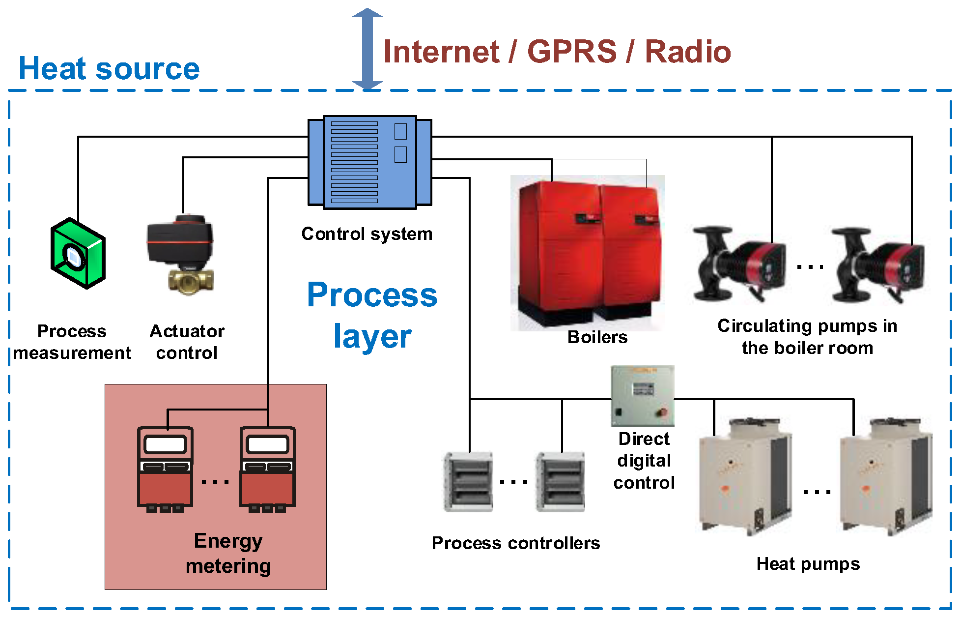
Figure 1. The scheme of the control system [25].
Technologies 13 00435 g001
Figure 2. Diagram of the heating circuit that was used as the data source for the 7-day daily gas consumption forecast.
Technologies 13 00435 g002
Figure 3. Raw data as a time series characterising over 11 years of gas consumption.
Technologies 13 00435 g003
Figure 4. Comparison of heating seasons. Daily gas consumption versus daily temperature.
Technologies 13 00435 g004
Figure 5. LR model of gas consumption-outdoor temperature.
Technologies 13 00435 g005
Figure 6. Graph of residuals after temperature model.
Technologies 13 00435 g006
Figure 7. A schematic of the Heisenberg boxes of the wavelet transform. (a) Sine function, (b) Window, (c) Mulitlication, (d) Wavelets, (e) Frequency distribution, (f) Heisenberg boxes.
Technologies 13 00435 g007
Figure 8. The scheme of the proposed LSTM model of a synthetic time series.
Technologies 13 00435 g008
Figure 9. Wavelet decomposition of chosen seasons. (a) 2014/2015, (b) 2019/2020, (c) 2020/2021 (due to COVID-19), and (d) 2023/2024.
Technologies 13 00435 g009
Figure 10. Ten seasons, variations of detail D1 and D2 waves.
Technologies 13 00435 g010
Figure 11. Ten seasons, variations of approximation waves.
Technologies 13 00435 g011
Figure 12. Results of nMAE (Graphical comparison of real values and synthetic data).
Technologies 13 00435 g012
Figure 13. Results of NRMSE (Graphical comparison of actual values and synthetic data).
Technologies 13 00435 g013
Figure 14. (a,b) Graphical comparison of one-week-ahead predicted value, varying component A1.
Technologies 13 00435 g014
Figure 15. (a,b) Graphical comparison of one-week-ahead predicted values, varying details D1 and D2.
Technologies 13 00435 g015
Figure 16. (a,b) Graphical comparison of one-week-ahead predicted values, varying details D5, D6.
Technologies 13 00435 g016
Figure 17. (a,b) Graphical comparison of one-week-ahead predicted values, without synthetic data.
Technologies 13 00435 g017
Figure 18. Comparison of training results and prediction of the 11th season. (a) Whole interval, (b) Details from i = 110 to i = 177.
Technologies 13 00435 g018
Figure 19. The scheme of the proposed LSTM model based on the individual wavelet LSTM models.
Technologies 13 00435 g019
Figure 20. (a) Training of the approximation wavelet component of residuals; (b) Its prediction for Season 11.
Technologies 13 00435 g020
Figure 21. Prediction of detail wavelets D1 of Season 11 residuals.
Technologies 13 00435 g021
Figure 22. Prediction of detail wavelets D2 of Season 11 residuals.
Technologies 13 00435 g022
Figure 23. Prediction of detail wavelets D3 of Season 11 residuals.
Technologies 13 00435 g023
Figure 24. Prediction of detail wavelets D4 of Season 11 residuals.
Technologies 13 00435 g024
Figure 25. Prediction of detail wavelets D5 of Season 11 residuals.
Technologies 13 00435 g025
Figure 26. Prediction of detail wavelets D6 of Season 11 residuals.
Technologies 13 00435 g026
Figure 27. (a) Predicted residuals (b) Predicted data of daily gas consumption. Both of them are compared to the actual values of Season 11.
Technologies 13 00435 g027
Figure 28. ECMWF model of time series interval from the 11th Season. Comparison of the 7-day temperature forecast and actual temperature on D-day.
Technologies 13 00435 g028
Figure 29. Graphical comparison of the prediction of 7-day gas consumption calculated based on the 7-day temperature forecast (LSTM method and LSTM–wavelet) with actual gas consumption.
Technologies 13 00435 g029
Figure 30. Comparison of the 7-day gas consumption forecast with actual gas consumption.
Technologies 13 00435 g030
Figure 31. Graphical comparison of the 7-day gas consumption forecast calculated based on the 7-day temperature forecast with actual gas consumption. Two methods are used.
Technologies 13 00435 g031
Table 1. Statistical evaluation of interesting data.
Heating Periods2014–20152015–20162016–20172017–20182018–2019
Number of days in heating period213214213213213
Absolute maximum (gas consumption)16381489157514531505
Absolute minimum (gas consumption)165247118137156
Mean of gas consumption 759.4747.8839.3781.3818.2
The standard deviation of gas consumption 309.4241.2310.6308.1324.1
Total gas consumption161,750160,030178,775166,411174,284
Absolute maximum (temperature)21.520.420.424.823.8
Absolute minimum (temperature)−4.8−5.0−10.4−6.0−2.7
Mean of temperature 9.08.86.88.39.3
The standard deviation of temperature5.45.06.36.46.1
Heating Periods2019–20202020–20212021–20222022–20232023–2024
Number of days in heating period214213213213214
Absolute maximum (gas consumption)12731353125110941279
Absolute minimum (gas consumption)1811292271150
Mean of gas consumption 740.9815.0794.0630.4650.4
The standard deviation of gas consumption 276.0236.0233.3252.6280.0
Total gas consumption158,559172,586169,123134,271138,539
Absolute maximum (temperature)21.321.321.219.223.1
Absolute minimum (temperature)−0.8−4.7−1.2−2.0−2.4
Mean of temperature 9.57.88.28.810.3
The standard deviation of temperature5.35.04.74.85.9
Table 2. Other results of linear regression.
SSE3.52 × 107
R20.798
RMSE126.61
Table 3. Results of nMAE (Comparison of real values and synthetic data) for chosen season.
nMAEOCTNOVDECJANFEBMARAPR
1st season,
variation of D1D2
0.1440.0850.1010.0590.0540.1160.114
1st season,
variation of D5D6
0.1040.0920.1200.1150.0330.0600.059
6th season,
variation of D1D2
0.1520.0780.0660.0470.0510.0660.130
6th season,
variation of D5D6
0.0570.0560.0570.0360.0300.0270.048
7th season,
variation of D1D2
0.1080.0600.0530.0460.0490.0510.070
7th season,
variation of D5D6
0.07130.0780.1160.0590.0360.0230.064
10th season,
variation of D1D2
0.1590.0600.1070.0600.0670.0820.136
10th season,
variation of D5D6)
0.0800.0530.1030.0610.0390.0370.081
Table 4. Results of NRMSE (Comparison of real values and synthetic data) for chosen season.
sMAPEOCTNOVDECJANFEBMARAPR
1st season,
variation of D1D2
0.0800.1200.1170.0800.1350.2110.117
1st season,
variation of D5D6
0.0580.1230.1460.1270.0860.1010.058
6th season,
variation of D1D2
0.1390.1620.1140.1230.1710.1400.117
6th season,
variation of D5D6
0.0530.1160.0960.0960.1010.0580.039
7th season,
variation of D1D2
0.0930.1100.1820.1220.0950.0970.097
7th season,
variation of D5D6
0.0590.1390.3320.1550.0720.0430.077
10th season,
variation of D1D2
0.1770.1010.1020.1480.1460.1370.113
10th season,
variation of D5D6)
0.0870.0900.0950.1350.0940.0610.069
Table 5. Numerical Evaluation of Training Performance.
TrainingnMAENRMSE
Without synthetic data0.1780.154
Synthetic data, varying
approximation A1
0.1840.159
Synthetic data, varying
D1 and D2 details
0.1710.148
Synthetic data, varying
D5 and D6 details
0.1890.156
Table 6. The computational cost for synthetic data training method and wave training method.
Step/OperationComplexity/Estimated Cost of Synthetic Data Training MethodComplexity/Estimated Cost of Wave Training Method
Data normalisation O ( n ) O ( n )
LSTM layer definition O ( 1 ) O ( 1 )
LSTM training O ( E · B · T · h 2 ) 7 O ( E · B · T · h 2 )
Prediction O ( T _ t e s t · h 2 ) 7 O ( T _ t e s t · h 2 )
Denormalization + linear correction O ( n _ t e s t ) O ( n _ t e s t )
Here, n is number of training samples, T is sequence length (here number of training samples), h is number of hidden units in LSTM layer, E is number of epochs, and B is number of batches. The computational costs reported are comparable; however, as the second method did not employ synthetic data, the total costs were approximately reduced by half.
Disclaimer/Publisher’s Note: The statements, opinions and data contained in all publications are solely those of the individual author(s) and contributor(s) and not of MDPI and/or the editor(s). MDPI and/or the editor(s) disclaim responsibility for any injury to people or property resulting from any ideas, methods, instructions or products referred to in the content.