Abstract
Irrigation is crucial for crop cultivation and productivity. However, traditional methods often waste water and energy due to neglecting soil and crop variations, leading to inefficient water distribution and potential crop water stress. The crop water stress index (CWSI) has become a widely accepted index for assessing plant water status. However, it is necessary to forecast the plant water stress to estimate the quantity of water to irrigate. Deep learning (DL) models for water stress forecasting have gained prominence in irrigation management to address these needs. In this paper, we present a comparative study between two deep learning models, ConvLSTM and CNN-LSTM, for water stress forecasting using remote sensing data. While these DL architectures have been previously proposed and studied in various applications, our novelty lies in studying their effectiveness in the field of water stress forecasting using time series of remote sensing images. The proposed methodology involves meticulous preparation of time series data, where we calculate the crop water stress index (CWSI) using Landsat 8 satellite imagery through Google Earth Engine. Subsequently, we implemented and fine-tuned the hyperparameters of the ConvLSTM and CNN-LSTM models. The same processes of model compilation, optimization of hyperparameters, and model training were applied for the two architectures. A citrus farm in Morocco was chosen as a case study. The analysis of the results reveals that the CNN-LSTM model excels over the ConvLSTM model for long sequences (nine images) with an RMSE of 0.119 and 0.123, respectively, while ConvLSTM provides better results for short sequences (three images) than CNN-LSTM with an RMSE of 0.153 and 0.187, respectively.
Keywords:
water stress; arboriculture; CWSI; time series; forecasting; deep learning; remote sensing; ConvLSTM; CNN-LSTM 1. Introduction
Water stress, stemming from inadequate water supply and decreased precipitation, poses significant challenges to agricultural productivity, plant health, and environmental sustainability [1,2]. Traditional irrigation practices often lead to excessive water usage and inefficient distribution due to neglecting soil and crop variability [3]. To address these challenges, plant water stress forecasting combined with the crop water stress index (CWSI) has become an important tool for irrigation management, since this index is a widely accepted indicator for quantifying plant water status [4,5,6]. It is calculated based on plant temperature measurements and temperature baselines, enabling farmers to assess crop water stress levels and make informed irrigation decisions. Numerous studies highlighted the significance of CWSI in irrigation scheduling, demonstrating that maintaining specific CWSI thresholds before irrigation can optimize yield and water conservation for various crops [7].
The use of the CWSI along with thermal information goes back to the 1960s, with the introduction of infrared thermal sensors at ground level [8] and the development of CWSI [5]. The CWSI has become the main indicator for assessing plant water status [9]. Additionally, applying it over large areas to detect water stress has gained momentum more recently with the technological advancement and integration of high-resolution thermal cameras on manned aerial vehicles [10].
Deep learning models have proven effectiveness in extracting complex patterns from spatial and temporal data, making them appropriate for tasks like water stress forecasting [11,12]. The long short-term memory (LSTM) network, a variant of recurrent neural networks (RNNs), has demonstrated remarkable performance in time-series predictions by overcoming the vanishing gradient problem faced by traditional RNNs [13,14].
The integration of LSTM with convolutional neural networks (CNNs) has gained more interest due to their complementary strengths in handling spatial and temporal information. Architectures such as convolutional LSTM (ConvLSTM) and CNN-LSTM have shown promising results in diverse applications ranging from traffic pattern forecasting and precipitation nowcasting [15,16] to agricultural tasks such as crop yield prediction, classification, and mapping using satellite imagery [17,18,19].
Considering the alarming water stress situation in Morocco, the need for innovative solutions to optimize agricultural water usage becomes imperative due to the importance of agricultural activity, which is a key pillar of the Moroccan economy. The World Resources Institute has recognized Morocco as one of the countries most affected by water stress, such that by 2040, the level of water stress will reach 80%, which is too high for an agricultural country for which agriculture consumes 73% of its water resources [20].
Considering these challenges, this article presents a comprehensive comparative study of two interesting DL models that combine LSTM and CNN, ConvLSTM and CNN-LSTM, for water stress forecasting. A citrus farm in Morocco was chosen as a case study.
The remaining sections of this paper are organized as follows: Section 2 presents the previous related studies that addressed the issue of evapotranspiration and crop water stress using DL architectures. Section 3 gives an overview of the methodology adopted in our study. Section 4 details the case study. In this section, we present the study area, the data used, the implementation steps of the two DL models, ConvLSTM and CNN-LSTM, and the validation approach. Section 5 presents the results and discussion. Section 6 concludes this paper.
2. Related Works
Table 1 lists the main studies that focused on the use of DL models to predict evapotranspiration. The studies presented in this table illustrate the application of several DL architectures, such as LSTM (long short-term memory), ConvLSTM (convolutional LSTM), and other variants, to specifically address the challenges of evapotranspiration.

Table 1.
Overview of studies exclusively using deep learning models to predict evapotranspiration and water stress.
The utilization of data such as atmospheric variables in addition to soil moisture leads to satisfactory predictions of evapotranspiration (ETa). The LSTM model stands out particularly in utilizing this type of data, showcasing a remarkable capacity for making short- and medium-term predictions. However, it is noteworthy that the precision of LSTM models slightly decreases with an increase in the forecast horizon. Additionally, a crucial aspect links the models’ performances to atmospheric data and their respective climatic conditions. This is especially relevant in the case of Reference [23], where the LSTM model outperforms the NARX model when using data from areas with subtropical climates, while for data originating from semi-arid climate zones, the NARX model exhibits better performance. This demonstrates that the utilization of the model heavily depends on the project’s objectives and the type of data used.
Upon closer examination of emerging research trends, it becomes evident that the usage of hybrid models holds a significant place. This inclination toward hybrid models stems from their inherent ability to combine the strengths and features of different architectures, often resulting in improved performance compared to traditional models. The study in [25] is particularly enlightening in this regard. It highlights the potency of a specific hybrid model, the CNN-GRU, in comparison to simpler approaches like LSTM and GRU. This analysis showcases that the integration of features and elements from multiple models, such as convolutions and recurrent gates, can provide substantial added value in terms of performance and precision [25].
Furthermore, after analyzing Table 1, we observe that DL models show a slight superiority over machine learning models, as is the case in [30]. In addition, both DL and machine learning (ML) models outperform the empirical methods. However, there are situations where deep learning models perform slightly better. This confirms that the choice of the appropriate model depends on the data available and the objectives of this study. In conclusion, DL models remain the best performers overall.
In line with these observations, the importance of spatiotemporal forecasting is evident in anticipating future events by considering different temporal and spatial dimensions. This approach is crucial in several fields such as health, natural resource management, and natural event management as well as in the agricultural sector, which heavily depends on environmental variations. Providing accurate, clear, and spatially well-represented forecast allows for decision-makers to make informed decisions and develop strategies to better anticipate the consequences of phenomena that vary spatiotemporally. With the advancement of remote sensing techniques, several phenomena have become mapped over large geographical areas and with very high resolution (LULC, change detection, sea level variation, urban growth, etc.). Remote sensing images provide rich information thanks to their continuous representation and multispectral bands. Several DL architectures have been developed to perform spatiotemporal forecasting of different phenomena based on remote sensing images. Among the most robust models, we find (ConvLSTM) and the hybrid model CNN-LSTM. Authors in [31] demonstrated the robustness and high accuracy of ConvLSTM in their forecasts of NDVI values in diversified locations. With an RMSE obtained of 0.0798 for the NDVI forecasts in soybean fields, ConvLSTM outperformed the best configuration for the parametric growth model of soybean (PCGM), which recorded a higher RMSE of 0.0992 for the same fields. The architecture of ConvLSTM, based on convolutional neural networks, is particularly suitable for the input and output of image data. Unlike RNNs, ConvLSTM simplifies the integration process and is efficient for accurately predicting images of varying sizes, even with a reduced training data size. In other research, the ConvLSTM showed high performance in a study conducted by [32] in the South and East China Seas to forecast significant wave height (SWH). The results showed that ConvLSTM could be applied with great precision and efficiency. For more complex forecasts, such as the El Niño–Southern Oscillation (ENSO), which is identified by the El Niño oceanic index (ONI) and characterized by sea surface temperature (SST), the complexity of this model lies in its characterization based on SST anomalies in the tropical Pacific. For this problem, ConvLSTM-RM was developed [33]. This hybrid model combines convolutional LSTM and a rolling mechanism to solve the spatiotemporal forecasting problem of ENSO. Over multiple time intervals, the model outperformed the other tested methods.
In the context of spatiotemporal forecasting of evapotranspiration, there are fewer studies using raster data and the ConvLSTM. In a study presented by [21], ConvLSTM was effectively used for evapotranspiration predictions using MODIS sensor data. However, it is essential to note that ConvLSTM is not the only beneficial model for spatiotemporal forecasting. Other LSTM-based architectures such as CNN-LSTM and Stack-LSTM have yielded positive results. The study presented in [34] compared three forecasting LSTM models based on Sentinel-1 image time series, and they found that ConvLSTM was not recommended when image sizes and sequence lengths increased. Although the CNN-LSTM and Stack-LSTM models gave good results, their processing time was significantly higher than that of ConvLSTM due to the convolution operations used. These results highlight the need to carefully consider the specific requirements of a given task when choosing between different LSTM-based architectures.
This work provides an in-depth look at the performance, advantages, and limitations of ConvLSTM and CNN-LSTM models when applied to crop water stress in agriculture. Our focus is to describe the full pipeline of implementing these two DL models that encompasses data preprocessing, hyperparameters finetuning, model training, and forecasting. In addition, we proceed to a comprehensive comparison of the performance of these two DL models to assess their efficiency.
3. Methodology
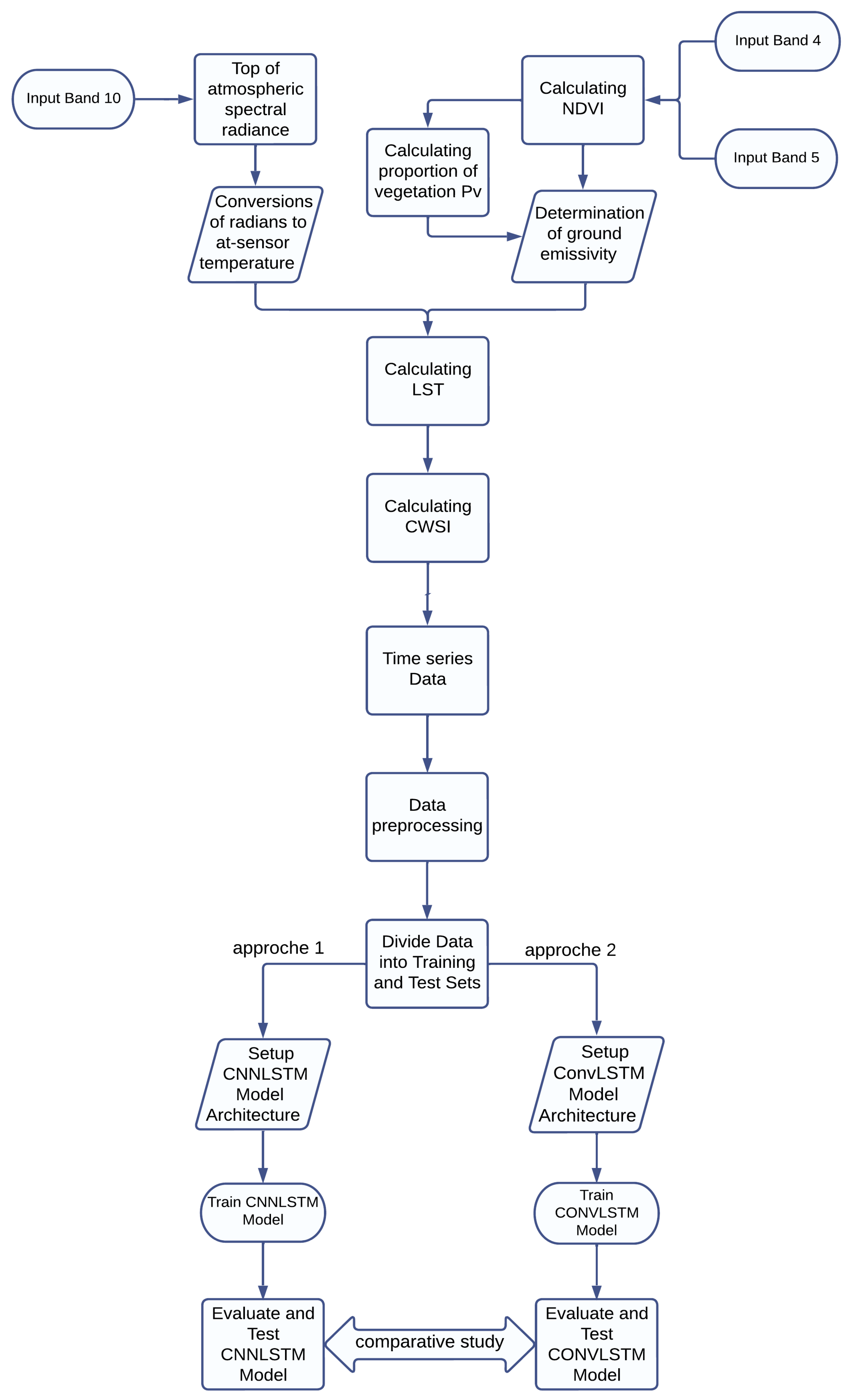
The proposed methodology consists, first of all, in preparing a dataset allowing for the exploitation of DL models for the forecasting of crop water stress. This dataset was created using the Google Earth Engine platform, capturing a time series of images classified by using the crop water stress index (CWSI) during the period from 2015 to 2023. The imagery dataset comprises 50 Landsat 8 images of the study area, each collected at 2-month intervals. The data preprocessing phase started with the conversion of these GEOTIFF format images into numerical matrices with the NPY extension, enabling seamless data loading, sequence preparation, and the division of the dataset into training and test sets. After that, the two models were implemented. The fine tuning, training, and comparative analysis of the two models, ConvLSTM and CNN-LSTM, were carried out to assess their relevance in crop water stress forecasting. Figure 1 illustrates the proposed methodology encompassing data preparation and preprocessing, model configuration, training, and comparison.
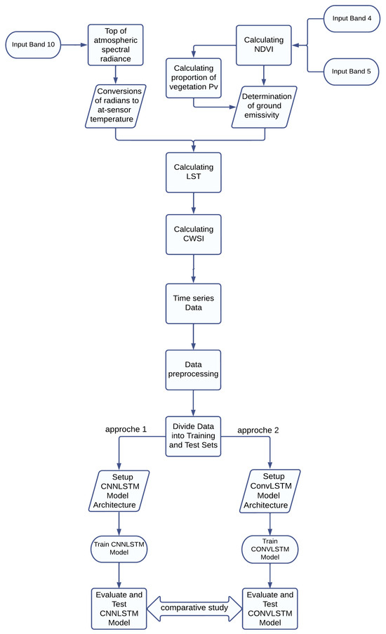
Figure 1.
A flowchart visualizing the comprehensive methodology adopted.
This description highlights the main steps and underlying logic of the process, while further details are provided in the following section.
4. Case Study
4.1. Study Area
The study area for this research is an irrigated citrus farm, known as Ourgha Farm, situated in the Khnichet rural commune in the Sidi Kacem province of western Morocco, part of the Rabat-Salé-Kénitra region (Figure 2). The geographic coordinates of the farm are 34°26′44.769″ N latitude and 5°41′30.117″ W longitude. Ourgha Farm covers an area of approximately 500 hectares and is divided into several parcels that feature a variety of citrus species. Irrigation at the farm is primarily drip-based, facilitated by rainfall and the nearby Ourgha River. The region experiences a semi-arid Mediterranean climate with average winter temperatures of 12.5 °C, summer temperatures of 25.2 °C, and an average annual precipitation of 685 mm, as per ORMVAG data. In the Khnichet commune, irrigated areas account for 41% of the total area.
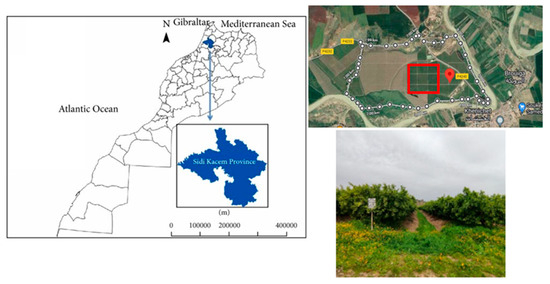
Figure 2.
Geographical location and delimitation of the “Ourgha” farm in Morocco.
4.2. Data
Data used in the research were procured from the Landsat 8 Collection 2 Tier 1 DN value series, which represents scaled, calibrated at-sensor radiance. These are high-quality Landsat scenes deemed suitable for time-series processing analysis. The data, part of Tier 1, includes Level-1 Precision Terrain (L1TP) processed data, characterized by reliable radiometry and intercalibration across different Landsat sensors. The georegistration of Tier 1 scenes maintains consistent accuracy within prescribed tolerances (≤12 m root mean square error (RMSE)). This consistency ensures that all Tier 1 Landsat data, regardless of the sensor, are intercalibrated across the full collection. Data were retrieved and computations were executed using Google Earth Engine.
To classify Landsat 8 images using the crop water stress index (CWSI), the process involves several key steps. First, the top-of-atmosphere (TOA) spectral radiance of the thermal band (Band 10) must be calculated, using specific formulas provided by the USGS.
Lλ = ML * Qcal + AL
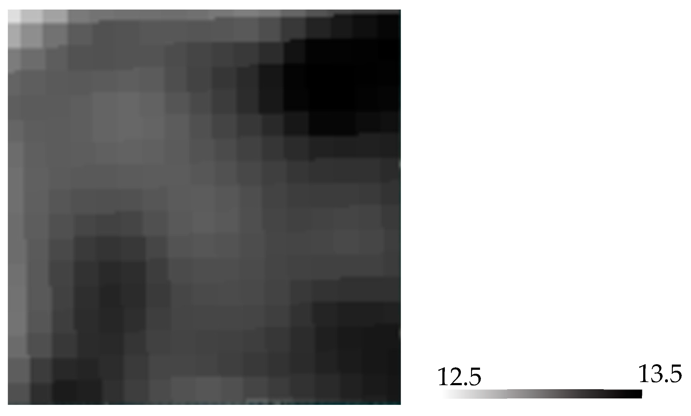
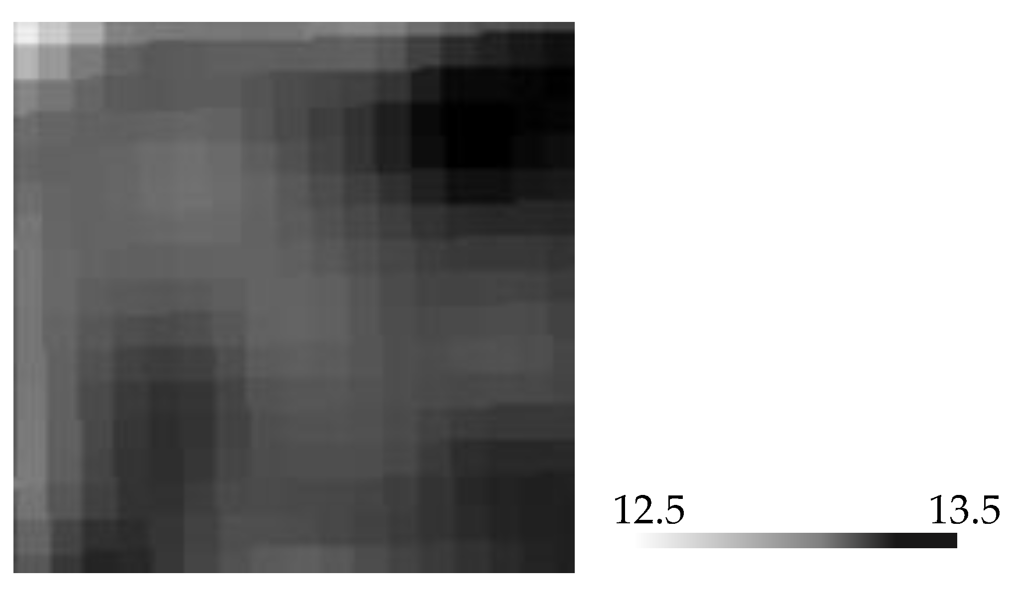
Once the pixel numeric values are converted to radiance, the thermal infrared sensor (TIRS) band data needs to be further processed to obtain the brightness temperature (BT) values as shown in Figure 3.
BT = K2 * ln[(K1/Lλ) + 1] − 273.15
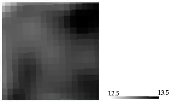
Figure 3.
Brightness temperature (BT) values in Celsius.
Next, the red and near-infrared bands of Landsat are employed to compute the normalized difference vegetation index (NDVI) as shown in Figure 4.
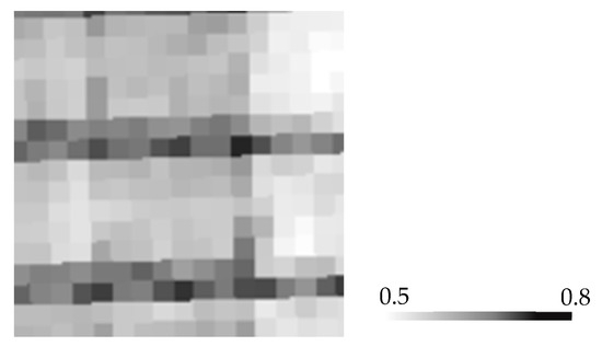
Figure 4.
Normalized difference vegetation index (NDVI) values.
NDVI calculation is essential as it is used to assess the proportion of vegetation (PV), crucial for determining soil emissivity based on NDVI, calculated vegetation proportion, and emissivity values for soil and vegetation.
The emissivity values obtained were and for vegetation and soil, respectively [35,36].
The NDVI is computed using the following formula [37]:
To calculate the proportion of vegetation (), we follow the method outlined in [38]. This approach suggests utilizing the NDVI values for vegetation ) and soil () in a global context [39]. The calculation is performed using the following formula:
The land surface temperature (LST), measured in degrees Celsius, is then calculated by adjusting the spectral radiance to the sensor brightness temperature (BT) based on spectral emissivity (Figure 5).

Figure 5.
Land surface temperature (LST) values.
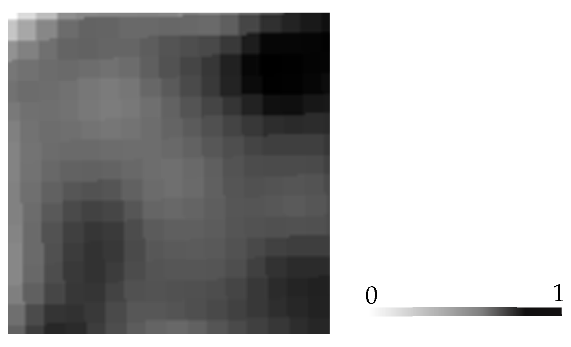
The final step in this approach involves calculating the CWSI, as shown in Figure 6, using the canopy temperature obtained from the calculated LST, along with temperatures from hot and cold pixels.

Figure 6.
Crop water stress index (CWSI) values.
CT represents the canopy temperature obtained from the computed land surface temperature (LST). and denote the temperatures derived from warm and cold pixels, respectively.
After validating the classification of images using the CWSI, the next step is to download a time series of classified images from 2015 to 2023, with a 2-month interval, from the Google Earth Engine platform. These images will be used to train and validate ConvLSTM and CNN-LSTM models.
In the data transformation and format conversion process, the initial step involves reading the crop water stress index images in our working environment. We utilize the “ReadAsArray()” function in the GDAL library to convert these 50 images in GEOTIFF format into matrices with the NPY extension, making the data compatible with the Numpy library. These matrices have dimensions (M, N, Channels), where “M” and “N” represent the rows and columns, respectively, while “Channels” signifies the image bands. In our case, the images are M = N = 18 with CHANNELS = 1, as we are working with a single index, crop water stress index, with values ranging from 0 to 1.
After obtaining the NPY matrices, we address “NaN” values by replacing them with the nearest neighbor pixel value, as water stress tends to vary in a continuous manner. We then proceed to load the data in NPY in a NumPy array representing CWSI time series with dimensions [Total_Data, M, N, Channels].
Next, we prepare sequences for our deep learning models, ConvLSTM and CNN-LSTM, which involve predicting the next image in a sequence from a given input sequence. These sequences are organized meticulously, creating two tensors: “Input_All” and “Output_All.” The former has dimensions (Number_Sequence, sequence_length, height, width, channels), where “Number_Sequence” represents the total number of sequences and “sequence_length” denotes the number of images in each sequence. The latter, “Output_All,” has dimensions (Number_Output, height, width, channels), with “Number_Output” representing the number of forecasted images.
Following sequence preparation, we divide the data into training and validation sets, allocating 80% for training and 20% for validation. This division is required for model evaluation, preventing overfitting, and ensuring generalization to unseen data.
Lastly, we conduct various tests to determine optimal model configurations. Different numbers of consecutive images per sequence were tested (3, 6, and 9), maintaining a consistent 2-month temporal interval between images. These tests help us understand how the lookback time impacts model performance and thus fine-tune the models for more accurate water stress forecasting.
4.3. CNN-LSTM Model Setup
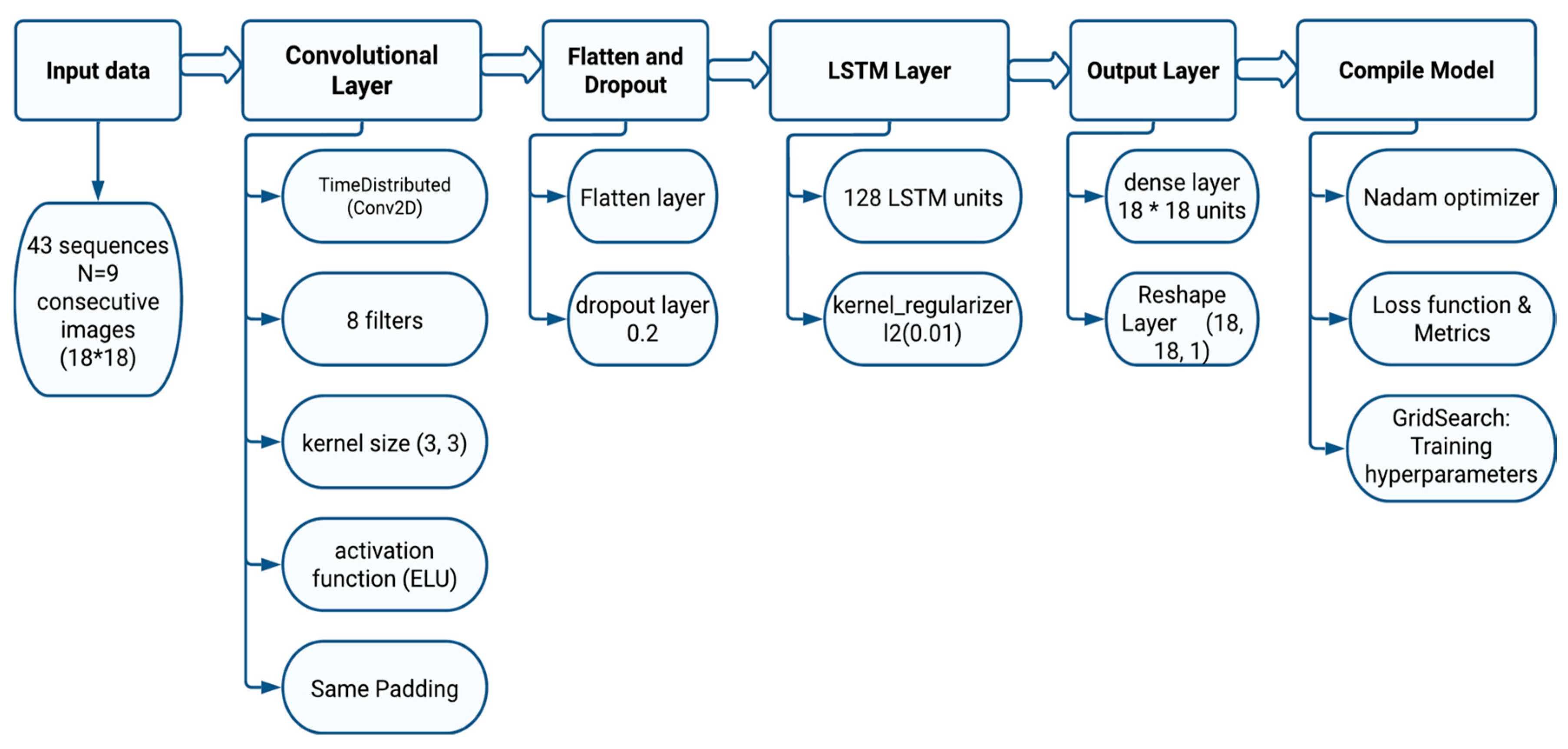
The first adopted model is based on the CNN-LSTM architecture (Figure 7). This model was used to process sequences of 2D images while effectively capturing spatial and temporal relationships. This CNN-LSTM architecture comprises multiple components that collaboratively achieve this complex task. The LSTM layer is used to capture the temporal dependencies in sequential data.

Figure 7.
Illustration of the proposed CNN-LSTM neural network architecture.
- Input Data:
The proposed model requires a sequence of 2D images with a dimension18 × 18 pixels representing CWSI vegetation index. The “None” dimension in the input shape accommodates variable sequence lengths. This input consists of 43 sequences, each containing 9 18 × 18 pixel grayscale consecutive images.
- Convolutional Layer:
The initial step involves the application of a convolutional neural network (CNN) to each image within the sequence with an exponential linear unit (ELU) activation function to capture relevant information from the images. An ELU activation has been found to mitigate issues like vanishing gradients during training. One key aspect that distinguishes our approach is the use of “same” padding during the convolutional operation. Padding involves adding extra pixels to the edges of the images before applying convolutions. “Same” padding ensures that the output spatial dimensions (height and width) after the convolution operation remain the same as the input dimensions. This is crucial for maintaining congruence between the different images within a sequence and preserving their spatial relationships.
- Flatten and Dropout:
Following the convolutional layer, a flatten layer to each output feature map is applied. The flatten layer reshapes the multi-dimensional feature maps into a one-dimensional vector. This transformation turns the 3D tensor into a 1D vector for each time step. In our case, the original input consists of images with dimensions 18 * 18 * 1 (width * height * channels). After applying the flatten layer, which reshapes the data, each of these images is converted into a 1D vector of length 18 * 18 * 1 = 324. To counter overfitting, we introduced a dropout layer. Overfitting occurs when a neural network becomes too specialized in the training data, performing well on it but struggling with new, unseen data. The dropout layer helps alleviate this by strategically deactivating a portion of the units (neurons) within the flattened vectors. During training, for each update, a random subset of these units is temporarily “dropped out” or ignored, along with their connections. This prevents the network from becoming overly reliant on specific neurons and encourages it to learn more robust and generalized features.
- LSTM Layer:
Long short-term memory recurrent networks (LSTMs) were developed to overcome the vanishing and exploding gradient issues faced by standard recurrent neural networks (RNNs) as layers increase [40]. LSTMs, equipped with three gates—forget, input, and output—have the capability to retain and manage sequential data (Figure 8). The forget gate, determined by a sigmoid function, selectively discards or retains information based on its weight, crucially impacting the memory retention process. Meanwhile, the input gate, composed of sigmoid and tanh layers, updates the LSTM model’s memory by combining the previous hidden state and the current input. This updated memory state, influenced by both forget and input gates, is calculated using a specific equation. Finally, the output gate, employing a sigmoid layer, determines which part of the memory contributes to the output, producing the final output at each time step [40].
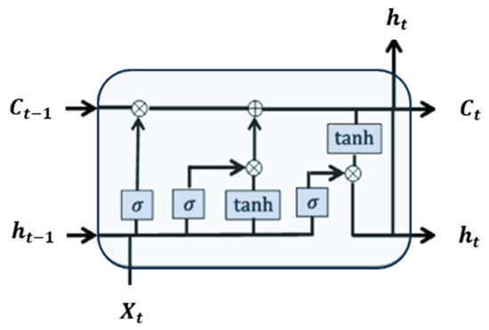
Figure 8.
The Long Short-Term Memory (LSTM) architecture.
Central to our architecture is the LSTM layer. This pivotal layer assimilates sequences of flattened vectors as input, utilizing its memory cells to effectively capture and learn intrinsic temporal dependencies in sequential data. With 128 LSTM units, this layer strategically employs input, forget, and output gates as explained previously. By doing so, the layer becomes adept at capturing intricate, long-term dependencies that span across the entire sequence of data. To ensure that our model generalizes well and does not become overly tailored to the training data, we introduce a technique known as L2 regularization to the LSTM kernel. L2 regularization operates by adding a penalty term to the loss function of the model to reduce the risk of overfitting. This penalty term is proportional to the square of the magnitudes of the weights in the LSTM kernel.
- Output Layer:
The output layer of our architecture is designed to provide meaningful forecasting based on the processed data. This layer consists of two key components: a dense layer with dimensions 18 × 18 and a reshaped layer that transforms the output into the desired format of 18 × 18 × 1. The dense layer is a fully connected layer that takes the representations learned from the preceding layers and maps them to the desired output shape of 18 × 18. Following the dense layer, we incorporate the reshape layer to reformat the output. The dense layer produces a 1D vector of length 18 * 18 = 324. However, since our ultimate goal is to generate images with dimensions 18 × 18 × 1, we use the reshape layer to transform this vector back into a 2D grid with the desired channel depth of 1. This reshaping process maintains the spatial arrangement of the data, ensuring that the output is consistent with the original image dimensions.
- Compile Model:
We compile our architecture using the Nadam optimizer and a set of metrics, encompassing mean squared error (MSE), root mean squared error (RMSE), and mean absolute error (MAE). The Nadam optimizer combines the benefits of Nesterov accelerated gradient (NAG) and adaptive moment estimation (Adam) algorithms. It incorporates NAG to enhance gradient-based updates and Adam to adaptively adjust learning rates for different parameters. This optimizer aims to provide efficient convergence during training by effectively handling the optimization process.
- Optimization of Hyperparameters and Model Training:
To optimize the hyperparameters of the CNN-LSTM model, a semi-automatic approach was adopted. Initially, we determined the appropriate ranges for each hyperparameter using our prior knowledge and preliminary experiments. The ranges of hyperparameters chosen for CNN-LSTM were the following:
- -
- Sequences length: 3, 6, and 9 images.
- -
- Activation function: ELU.
- -
- Epoch: 10, 30.
- -
- Learning rate: 10−4, 10−3, 10−2, 10−1.
- -
- Batch size: 1, 10.
- -
- Filters: 8, 32.
Then, the GridSearch algorithm was used to choose the best combination of hyperparameters. The cross-validation process applied is k-fold with a value of k equal to 3. Once the hyperparameters had been semi-automatically adjusted, we trained the CNN-LSTM model with CWSI spatiotemporal images to forecast subsequent images.
4.4. ConvLSTM Model Setup
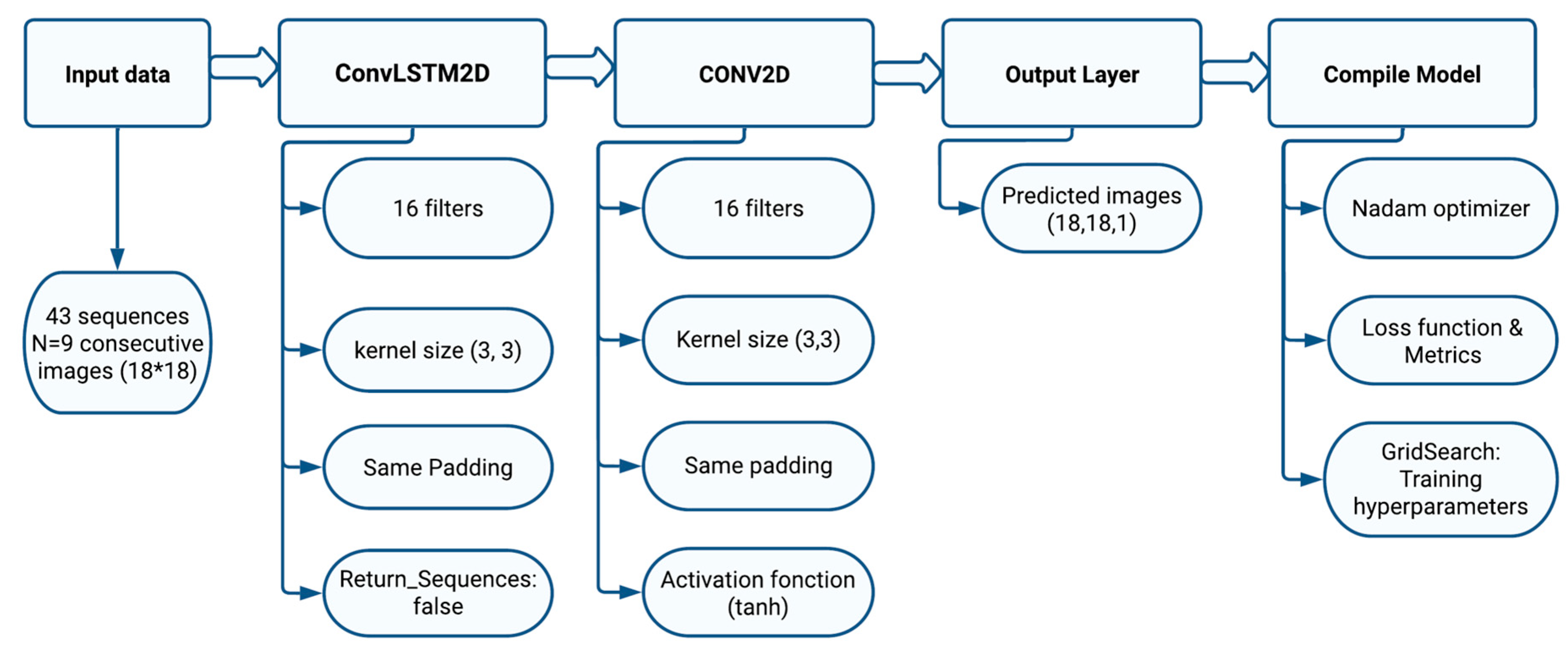
We employed ConvLSTM architecture (Figure 9), a sophisticated neural network model, to process 2D image sequences in such a way as to efficiently capture spatial and temporal relationships. This comprehensive architecture integrates various components that work in concert to accomplish this complex task. At the heart of the architecture is the ConvLSTM layer, a powerful innovation for modeling spatial and temporal dependencies in sequential data.
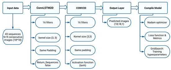
Figure 9.
Illustration of the proposed ConvLSTM neural network architecture.
- Input data: Identical to the input data utilized in the CNN-LSTM model.
- ConvLSTM2D:
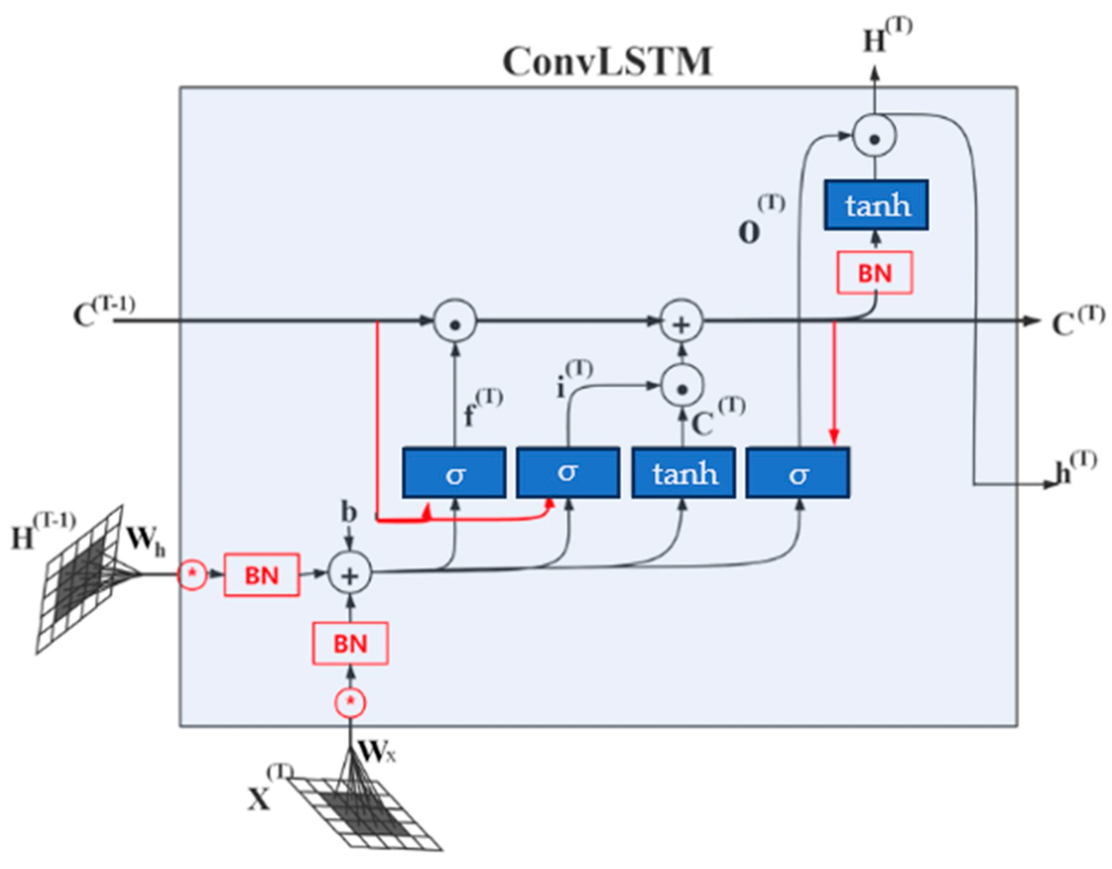
The ConvLSTM2D layer (convolutional long short-term memory 2D) combines the advantages of LSTM (long short-term memory) networks and convolution layers to process 2D sequential data (Figure 10). This layer is commonly used in image or video sequence processing tasks, where both spatial and temporal information is important. The following hyperparameters must be considered for the ConvLSTM2D Layer:
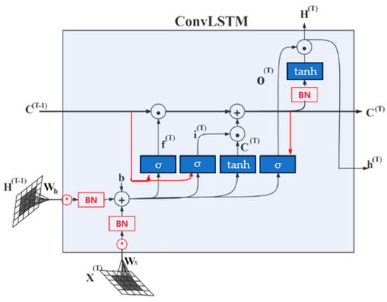
Figure 10.
ConvLSTM architecture.
Number of filters: Defines the number of filters used to extract features from the input data. The higher the number of filters, the more complex features the layer can learn, but it can also make the model more complex.
Kernel size: Specifies the size of the convolutional filters that are applied to the sequential input.
Padding.
Return sequences: In our model, this hyperparameter is set to false, meaning that the ConvLSTM2D layer produces a single output for each input sequence.
The ConvLSTM2D layer applies 2D convolution filters to recognize specific patterns, such as edges, textures, or other visual structures. In parallel with convolution operations, the ConvLSTM2D layer uses LSTM memory mechanisms to capture long-term sequential dependencies in the data. LSTMs are recurrent neural networks that store important information about past sequences and use it to influence the current output. This enables the model to consider the history of images in each sequence as follows:
Current input (xt): In ConvLSTM2D, xt represents the sequence image at time position t in the input sequence.
Previous hidden state (ht−1): ht−1 represents the hidden state at time position t−1. At the start of the sequence, ht−1 is usually initialized to a fixed value. At each subsequent time step, ht is updated according to the current input (xt) and the previous hidden state (ht−1) using LSTM memory mechanisms as explained for CNN-LSTM architecture.
LSTM mechanisms: The ConvLSTM2D layer uses LSTM memory mechanisms to combine xt and ht−1 and calculate ht, the hidden state at time position t. These mechanisms include gates (forget gate, input gate, and output gate) that regulate the flow of information in the LSTM unit. These gates enable the model to decide what information is important to retain and what to forget about the hidden state.
Output (ht): Once ht has been calculated, it is used to generate the output of the ConvLSTM2D layer at this time step. The dimensions of ht−1 are batch size, height, width, and channels.
This process is repeated for each time step in the sequence, where xt represents the image at that step and ht−1 is the state calculated from the previous step. This allows for the model to take into account the evolution of the image sequence over time, and to capture long-term sequential dependencies in the data.
- Conv2D:
The Conv2D layer is a two-dimensional convolution layer used mainly after the ConvLSTM2D layer, as it plays an essential role in processing the information extracted by the ConvLSTM2D layer at each time step of the sequence. It applies 2D convolution operations to the hidden state ht produced by the ConvLSTM2D layer. These convolution operations enable further exploration of the spatial characteristics of the hidden state, identifying important patterns and structures. In our case, the Conv2D layer produces an output that is an 18 * 18 image with a single channel that corresponds to a shape (18, 18, 1) representing the forecasted image.
- Compile Model, Optimization of Hyperparameters, and Model Training:
The same processes of model compilation, optimization of hyperparameters, and model training used in the CNN-LSTM were applied to the ConvLSTM architecture. The ranges of hyperparameters chosen for ConvLSTM are the following:
- -
- Sequences length: 3, 6 and 9 images.
- -
- Activation function: tanh.
- -
- Epoch: 10, 20, 1000, 1500, 2000.
- -
- Learning rate: 10−5, 10−4, 10−3, 10−2, 10−1.
- -
- Batch size: 1, 10.
- -
- Filters: 32.
Similarly to CNN-LSTM, the cross-validation process applied for ConvLSTM is k-fold with a value of k equal to 3.
4.5. Validation of CNN-LSTM and ConvLSTM Models
To validate the proposed CNN-LSTM and ConvLSTM models, we adopted an integrated approach combining quantitative measurements with visual assessments to ensure the robustness of our forecasting. We used several well-established performance metrics, including the following:
Mean square error (MSE): The loss function MSE measures the average squared prediction error between the observed and forecasted values . A low MSE implies a low error.
Root mean square error (RMSE): Another loss function is the RMSE, which defines the square root of the average squared prediction error between the observed and forecasted values. A smaller RMSE value implies a lower error.
Mean absolute error (MAE): A loss function that computes the prediction error between the observed and forecasted values. A small average deviation value of the AME is desired.
These indicators enable us to quantify precisely and systematically the deviation between the values predicted by our models and the actual values. This quantitative approach gives us a comprehensive overview of our models’ performance in terms of accuracy and ability to capture complex spatiotemporal variations.
In parallel, we perform visual validation by visually comparing the predicted images generated by our two models with the corresponding real images. This visual evaluation enables us to assess the quality and qualitative adequacy of our model forecasting in relation to observed reality. It also enables us to detect any inconsistencies or errors that might not be captured by quantitative measurements alone.
By combining the quantitative and visual methods, we achieve a holistic understanding of our models’ performance in forecasting water stress. This approach enables us to better grasp the advantages and limitations of the CNN-LSTM and ConvLSTM models in modeling complex spatiotemporal patterns and producing accurate forecasts. Ultimately, this validation methodology reinforces confidence in the ability of our models to deliver reliable and meaningful results for CWSI-based water stress forecasting.
5. Results and Discussion
5.1. Results Overview
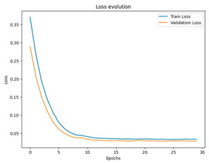
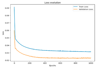
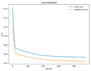
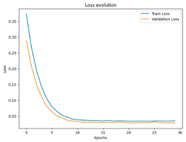
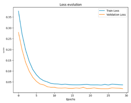
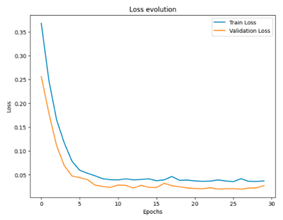
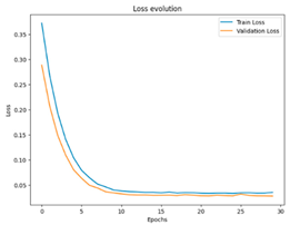
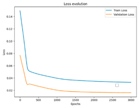
To summarize the results of this study, we compiled a summary table showing the best performances obtained for each scenario, in terms of optimal hyperparameters, together with the corresponding RMSE, MSE, and MAE values. This table provides an overview of the significant improvements brought about by semi-automatic hyperparameter tuning compared to the initial configurations. In addition, for a more concrete visualization of the effectiveness of our models, we included graphs representing the training and validation curves for each scenario. These curves highlight the convergence of the training and generalization capabilities of the models across the different iterations, providing a visual understanding of their performance.

Table 2.
Summary of best ConvLSTM model performance and hyperparameters.

Table 3.
Summary of best CNN-LSTM model performance and hyperparameters.
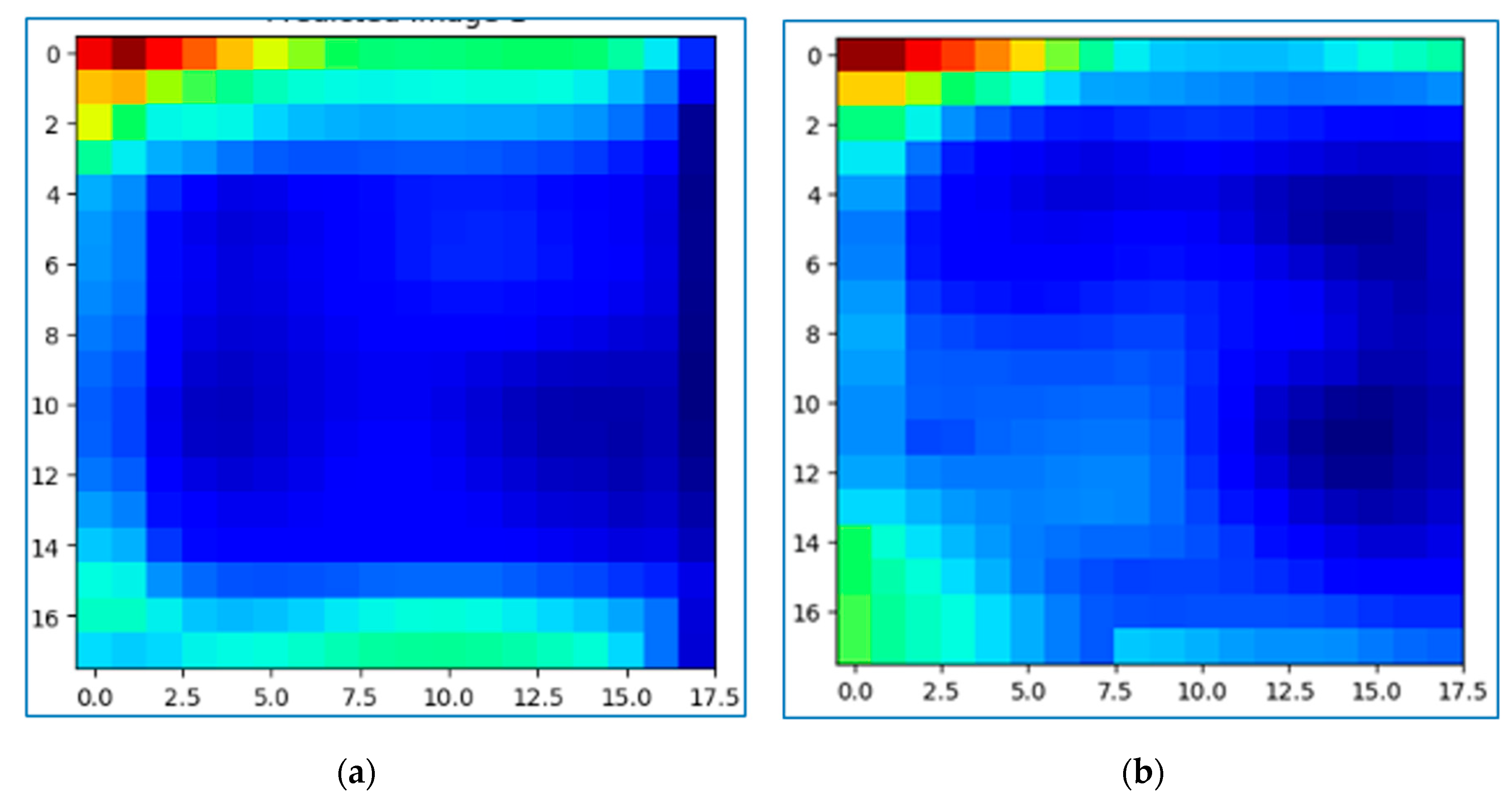
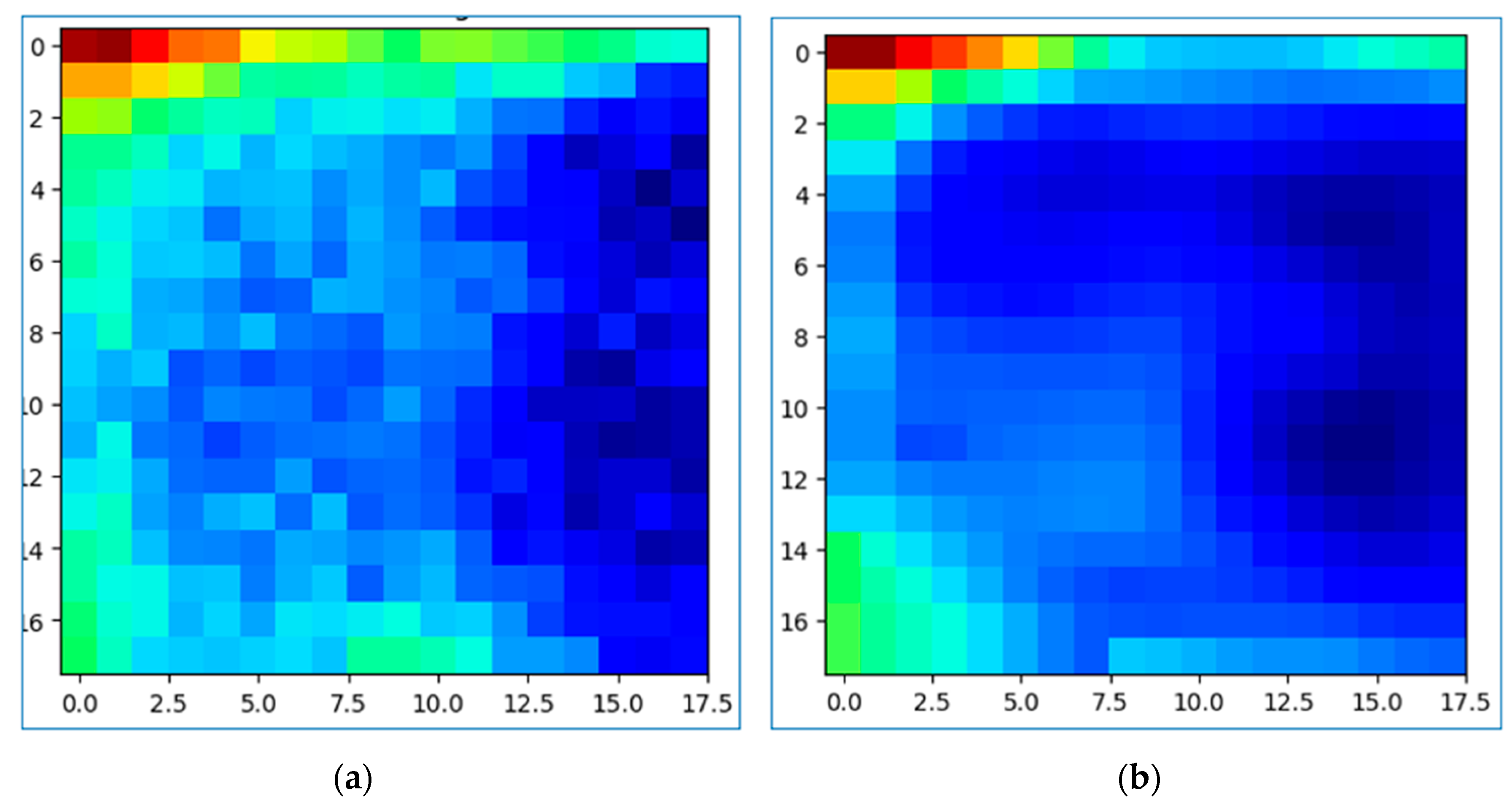
The best result achieved with an RMSE of 0.124 at a sequence length of nine images and its corresponding output image (Figure 11):
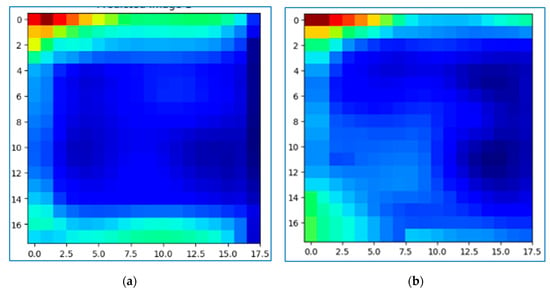
Figure 11.
(a) Forecasted CWSI image by ConvLSTM of 24 April 2023; (b) actual CWSI Image of 24 April 2023.
A visual comparison of the forecasted CWSI by ConvLSTM (Figure 11a) with the actual CWSI image (Figure 11b) shows that the general spatial pattern of water stress distribution is well captured. In addition, the forecasted CWSI image exhibits a more uniform distribution of CWSI values, whereas the actual image shows more localized variations and hotspots. This comparison suggests that while the ConvLSTM model can effectively capture the overall spatial pattern, the forecasting of finer nuances and complexities of the real-world data is more challenging. As detailed in Section 5.2, quantitative metrics could provide a comprehensive assessment of the performance of ConvLSTM in forecasting the CWSI.
The best result achieved with an RMSE of 0.119 at a sequence length of nine images and its corresponding output (Figure 12):

Figure 12.
(a) Forecasted CWSI image by ConvLSTM of 24 April 2023; (b) actual CWSI Image of 24 April 2023.
Similarly to ConvLSTM, the CNN-LSTM model was able to forecast the general spatial pattern of water stress distribution (Figure 12.a) compared to the actual CWSI image (Figure 12.b). However, the CWSI forecasted with CNN-LSTM presents less smoothness compared to ConvLSTM. Additionally, the CNN-LSTM model appears to overestimate the extent of high stress regions compared to the actual data. Section 5.2 provides more insights on the performance of ConvLSTM and CNN-LSTM based on quantitative metrics.
Based on the results presented in Table 2 and Table 3, a comparison of the best forecast model for CNN-LSTM and ConvLSTM is presented in Table 4.

Table 4.
Comparison of the best forecast results for each model.
The analysis of MSE, RMSE, and MAE obtained from using CNN-LSTM and ConvLSTM models to predict water stress shows that the CNN-LSTM model displays a slightly lower value than the ConvLSTM model. Both models demonstrate similar good performance with a slightly better performance of CNN-LSTM in terms of accuracy. In the next section, a more in-depth comparison between CNN-LSTM and ConvLSTM is presented.
5.2. Comparison of CNN-LSTM and ConvLSTM for CWSI Forecasting
As we are comparing two different models for forecasting spatiotemporal prediction of water stress, accuracy is not the only criterion to consider assessing the model’s reliability.
- Complexity and processing time:
As the results of Table 5 clearly show, the ConvLSTM model requires considerably more time to train, regardless of the scenario chosen (whether three, six, or nine images per sequence). This observation underlines the intrinsic complexity of the ConvLSTM model, as well as the sensitivity of its performance to the specific hyperparameters associated with it.

Table 5.
The training time for each model in the different scenarios.
To illustrate the difference in training times, let us consider the scenario of nine images per sequence. The ConvLSTM model requires 3000 epochs to achieve satisfactory results, while the CNN-LSTM achieves the equivalent performance in just 30 epochs. This disparity in training time between the two models underlines the importance of considering time constraints when choosing a model. Hence, the computational time demand could be a major drawback of ConvLSTM, especially when fast training is imperative. On the other hand, the CNN-LSTM may prove more suitable for applications where training time efficiency is crucial.
- Smoothness of forecasted images:
In this section, we consider the CNN-LSTM and ConvLSTM Models that were trained on a sequence of nine images because they present the best metrics.
The ConvLSTM model generates an image with a certain homogeneity in the variations of CWSI values, while the images produced by CNN-LSTM display more pronounced variations between pixels. This observation could be interpreted as follows:
The image generated by ConvLSTM seems to smooth out CWSI variations, thus creating some spatial continuity. Although this may be beneficial in contexts where real data exhibit gentle variations, it may not correspond to the reality of our study, where stress hydric variations are more pronounced.
More pronounced variations in pixel values are present in images forecasted by CNN-LSTM. These variations could result from its greater sensitivity to local changes and specific environmental features. Even though these variations may appear less smooth visually, they might better reflect the actual fluctuations in stress hydric levels, especially when real data exhibit rapid changes and significant variations between pixels.
It is important to note that relying solely on visualization as a validation criterion is not sufficient. To obtain a comprehensive evaluation of the quality of predictions from both models, it is essential to consider quantitative performance metrics, especially the RMSE. While the image generated by ConvLSTM may show some continuity in CWSI variations between pixels, it is noteworthy that the RMSE of the image generated by CNN-LSTM is lower than that of ConvLSTM (in a sequence of nine images). This indicates that, from a numerical perspective, CNN-LSTM’s predictions align more closely with actual stress hydric values than those of ConvLSTM. This smaller value in RMSE for CNN-LSTM can be interpreted as a better quantitative fit with real data, despite the more pronounced visual variations we observed in the predicted image. Thus, it is possible that CNN-LSTM accurately captures rapid changes and fluctuations in stress hydric levels, which is crucial for many real-time forecasting applications.
- Accuracy of the models:
It is essential to compare the performance of the CNN-LSTM and ConvLSTM models in different scenarios, as shown in Table 6, for assessing their effectiveness in forecasting spatiotemporal water stress. It is important to note that results vary according to the scenario, particularly the number of images included in each sequence.

Table 6.
Table of metrics for the two models in the three scenarios.
In the scenario with three images per sequence, we observe that ConvLSTM displays slightly higher accuracy than CNN-LSTM. This means that in situations where sequences are shorter, ConvLSTM can better capture water stress trends.
However, when the number of images per sequence is increased to six, the performance of both models becomes comparable, with neither showing a clear superiority. This suggests that for sequences of moderate length, both models can be used with similar results.
The most interesting scenario is that with nine images per sequence, where CNN-LSTM shows a clear improvement in accuracy over ConvLSTM. This indicates that for longer sequences, with more temporal data, CNN-LSTM can better model complex variations in water stress.
Ultimately, the choice between CNN-LSTM and ConvLSTM will depend on the specific needs of your application and usage scenario. When working with short sequences, ConvLSTM may be preferable. However, for longer sequences and more accurate water stress predictions, CNN-LSTM seems to be the optimal choice. This analysis highlights the importance of considering sequence length when choosing a model for water stress forecasting.
5.3. Discussion
The results obtained in this study highlight the effectiveness of hybrid DL models, particularly ConvLSTM and CNN-LSTM, for spatiotemporal forecasting of crop water stress using remote sensing data. These findings align with previous studies and contribute to the scientific advancements that underscore the potential of DL architectures in crop water stress forecasting.
Consistent with the observations of [21,22,23], our study reinforces the superiority of deep learning models over traditional machine learning approaches in handling the complex spatiotemporal patterns present in remote sensing data. The ability of ConvLSTM and CNN-LSTM to capture both spatial and temporal dependencies within the data has proven advantageous for accurate forecasting of crop water stress.
Our results corroborate the findings of [24], who demonstrated the potential of deep learning models in evapotranspiration estimation using satellite imagery. However, our study extends these findings by exploring the comparative performance of two specific deep learning architectures, ConvLSTM and CNN-LSTM, in a spatiotemporal forecasting context.
While both models exhibited promising performance, the CNN-LSTM architecture demonstrated a slight edge in overall accuracy, aligning with the observations of [41] on the efficacy of convolutional neural networks in processing raster data. This advantage can be attributed to the CNN-LSTM’s ability to capture localized variations and rapid changes in crop water stress, as evident from the visual analysis of the forecasted images.
Notably, our findings regarding the computational efficiency of the CNN-LSTM model, particularly for longer sequences, are consistent with the literature on the computational demands of deep learning models [21]. This highlights the trade-off between model complexity and computational resources, a consideration that should guide model selection based on the specific application and resource constraints.
It is worth acknowledging that our study aligns with the research gap identified in the literature, where the incorporation of satellite images into deep learning-based evapotranspiration and water stress forecasting has been underrepresented. By leveraging remote sensing data and exploring the comparative performance of two advanced deep learning architectures, our work contributes to bridging this gap and advancing our understanding of the use of deep learning in irrigation applications.
6. Conclusions
In conclusion, addressing crop water stress in agriculture is critical for ensuring global food security and sustainable resource management. Our research highlights the critical importance of accurate water stress forecasting in mitigating the detrimental effects on crop growth, yield, and quality. By leveraging technological advancements, particularly deep learning techniques and satellite imagery data, we can enhance water management practices. Through the utilization of ConvLSTM and CNN-LSTM models, we have contributed to the integration of innovative tools for crop water stress forecasting. Our exclusive reliance on satellite imagery data enables near-real-time monitoring over large agricultural areas, empowering farmers with valuable decision-making support.
This study reveals the complexity of forecasting water stress in a spatiotemporal context. Model performance depends on factors such as sequence length and data complexity. On one hand, the length of image sequences can have a significant impact on the model performance. LSTM models, such as ConvLSTM, are designed to capture short-term temporal dependencies. In scenarios with short sequences (such as three images per sequence), ConvLSTM has an advantage, as it can better manage these dependencies. However, when sequence length increases (as with nine frames per sequence), CNN-LSTM, which combines convolution layers with LSTMs, can better capture complex patterns in the data. On the other hand, the characteristics of real data can vary in complexity. Hence, in scenarios where the data are less complex and have simple patterns, ConvLSTM may be more appropriate as it tends to smooth out variations. However, in scenarios where data exhibit more variations, CNN-LSTM performs better due to its ability to capture local details and rapid changes in crop water stress. Understanding the impact of these factors is important to adapt the model accordingly to obtain optimal results.
In essence, our research underscores the importance of technological innovation in addressing crop water stress challenges, offering hope for more efficient water management, enhanced food security, and a sustainable agricultural future.
Author Contributions
Conceptualization, I.B., Y.S., M.B. and R.Y.; Methodology, I.B., Y.S., M.B. and R.Y.; Validation, I.B., Y.S., M.B. and R.Y.; Formal analysis, I.B., Y.S., M.B. and R.Y.; Investigation, I.B., Y.S., M.B. and R.Y.; Resources, M.B. and R.Y.; Writing—original draft preparation, I.B., Y.S., M.B. and R.Y.; Writing—review and editing, I.B., Y.S., M.B. and R.Y.; Supervision, M.B. and R.Y.; Project administration, M.B.; Funding acquisition, M.B. All authors have read and agreed to the published version of the manuscript.
Funding
This work was supported by the Ministry of Higher Education, Scientific Research, and Innovation (Morocco) (Alkhawarizmi/2020/17); the Digital Development Agency of Morocco (DDA) (Alkhawarizmi/2020/17); and the Centre National pour la Recherche Scientifique et Technique (CNRST) of Morocco (Alkhawarizmi/2020/17).
Data Availability Statement
The data will be available upon a reasonable request from the corresponding author.
Conflicts of Interest
The authors declare no conflicts of interest.
References
- Bootsma, A.; Boisvert, J.B.; de Jong, R.; Baier, W. La Sécheresse et l’agriculture Canadienne: Une Revue Des Moyens d’action. Sci. Chang. PlanétairesSécheresse 1996, 7, 277–285. [Google Scholar]
- Jiménez, S.; Dridi, J.; Gutiérrez, D.; Moret, D.; Irigoyen, J.J.; Moreno, M.A.; Gogorcena, Y. Physiological, Biochemical and Molecular Responses in Four Prunus Rootstocks Submitted to Drought Stress. Tree Physiol. 2013, 33, 1061–1075. [Google Scholar] [CrossRef] [PubMed]
- Jamroen, C.; Komkum, P.; Fongkerd, C.; Krongpha, W. An Intelligent Irrigation Scheduling System Using Low-Cost Wireless Sensor Network Toward Sustainable and Precision Agriculture. IEEE Access 2020, 8, 172756–172769. [Google Scholar] [CrossRef]
- Gonzalez-Dugo, V.; Zarco-Tejada, P.J.; Fereres, E. Applicability and Limitations of Using the Crop Water Stress Index as an Indicator of Water Deficits in Citrus Orchards. Agric. For. Meteorol. 2014, 198–199, 94–104. [Google Scholar] [CrossRef]
- Idso, S.B.; Jackson, R.D.; Pinter, P.J.; Reginato, R.J.; Hatfield, J.L. Normalizing the Stress-Degree-Day Parameter for Environmental Variability. Agric. Meteorol. 1981, 24, 45–55. [Google Scholar] [CrossRef]
- Jackson, R.D.; Idso, S.; Reginato, R.; Pinter, P., Jr. Canopy Temperature as a Crop Water Stress Indicator. Water Resour. Res. 1981, 17, 1133–1138. [Google Scholar] [CrossRef]
- Adeyemi, O.; Grove, I.; Peets, S.; Domun, Y.; Norton, T. Dynamic Modelling of the Baseline Temperatures for Computation of the Crop Water Stress Index (CWSI) of a Greenhouse Cultivated Lettuce Crop. Comput. Electron. Agric. 2018, 153, 102–114. [Google Scholar] [CrossRef]
- Tanner, C.B. Plant Temperatures. Agron. J. 1963, 55, 210–211. [Google Scholar] [CrossRef]
- Poblete-Echeverría, C.; Espinace, D.; Sepúlveda-Reyes, D.; Zúñiga, M.; Sanchez, M. Analysis of Crop Water Stress Index (CWSI) for Estimating Stem Water Potential in Grapevines: Comparison between Natural Reference and Baseline Approaches. Acta Hortic. 2017, 1150, 189–194. [Google Scholar] [CrossRef]
- Sepulcre-Cantó, G.; Zarco-Tejada, P.J.; Jiménez-Muñoz, J.; Sobrino, J.; De Miguel, E.; Villalobos, F.J. Detection of Water Stress in an Olive Orchard with Thermal Remote Sensing Imagery. Agric. For. Meteorol. 2006, 136, 31–44. [Google Scholar] [CrossRef]
- LeCun, Y.; Bengio, Y.; Hinton, G. Deep Learning. Nature 2015, 521, 436–444. [Google Scholar] [CrossRef] [PubMed]
- Kim, T.-Y.; Cho, S.-B. Predicting Residential Energy Consumption Using CNN-LSTM Neural Networks. Energy 2019, 182, 72–81. [Google Scholar] [CrossRef]
- Hochreiter, S.; Schmidhuber, J. Long Short-Term Memory. Neural Comput. 1997, 9, 1735–1780. [Google Scholar] [CrossRef] [PubMed]
- Miao, K.; Han, T.; Yao, Y.; Lu, H.; Chen, P.; Wang, B.; Zhang, J. Application of LSTM for Short Term Fog Forecasting Based on Meteorological Elements. Neurocomputing 2020, 408, 285–291. [Google Scholar] [CrossRef]
- Liu, Y.; Zheng, H.; Feng, X.; Chen, Z. Short-Term Traffic Flow Prediction with Conv-LSTM; IEEE: Piscataway, NJ, USA, 2017; pp. 1–6. [Google Scholar]
- Shi, X.; Chen, Z.; Wang, H.; Yeung, D.-Y.; Wong, W.-K.; Woo, W. Convolutional LSTM Network: A Machine Learning Approach for Precipitation Nowcasting. Adv. Neural Inf. Process Syst. 2015, 28. [Google Scholar]
- Sun, J.; Di, L.; Sun, Z.; Shen, Y.; Lai, Z. County-Level Soybean Yield Prediction Using Deep CNN-LSTM Model. Sensors 2019, 19, 4363. [Google Scholar] [CrossRef] [PubMed]
- Rustowicz, R.M.; Cheong, R.; Wang, L.; Ermon, S.; Burke, M.; Lobell, D. Semantic Segmentation of Crop Type in Africa: A Novel Dataset and Analysis of Deep Learning Methods. In Proceedings of the IEEE/CVF Conference on Computer Vision and Pattern Recognition (CVPR) Workshops, Long Beach, CA, USA, 16–20 June 2019; pp. 75–82. [Google Scholar]
- Ji, S.; Zhang, C.; Xu, A.; Shi, Y.; Duan, Y. 3D Convolutional Neural Networks for Crop Classification with Multi-Temporal Remote Sensing Images. Remote Sens. 2018, 10, 75. [Google Scholar] [CrossRef]
- Aqueduct|World Resources Institute. Available online: https://www.wri.org/aqueduct (accessed on 1 April 2024).
- Babaeian, E.; Sidike, P.; Siddique, N.; Devabhaktuni, V.; Tuller, M. Application of Long Short-Term Memory Deep Learning for Forecasting of Evapotranspiration from Ground and Satellite Observations. In Proceedings of the ASA, CSSA, SSSA International Annual Meeting, Salt Lake City, UT, USA, 9 November 2021. [Google Scholar]
- Babaeian, E.; Paheding, S.; Siddique, N.; Devabhaktuni, V.K.; Tuller, M. Short- and Mid-Term Forecasts of Actual Evapotranspiration with Deep Learning. J. Hydrol. 2022, 612, 128078. [Google Scholar] [CrossRef]
- Granata, F.; Di Nunno, F. Forecasting Evapotranspiration in Different Climates Using Ensembles of Recurrent Neural Networks. Agric. Water Manag. 2021, 255, 107040. [Google Scholar] [CrossRef]
- Farooque, A.A.; Afzaal, H.; Abbas, F.; Bos, M.; Maqsood, J.; Wang, X.; Hussain, N. Forecasting Daily Evapotranspiration Using Artificial Neural Networks for Sustainable Irrigation Scheduling. Irrig. Sci. 2022, 40, 55–69. [Google Scholar] [CrossRef]
- Ahmed, A.A.M.; Deo, R.C.; Feng, Q.; Ghahramani, A.; Raj, N.; Yin, Z.; Yang, L. Hybrid Deep Learning Method for a Week-Ahead Evapotranspiration Forecasting. Stoch. Environ. Res. Risk Assess. 2022, 36, 831–849. [Google Scholar] [CrossRef]
- Chia, M.Y.; Huang, Y.F.; Koo, C.H.; Ng, J.L.; Ahmed, A.N.; El-Shafie, A. Long-Term Forecasting of Monthly Mean Reference Evapotranspiration Using Deep Neural Network: A Comparison of Training Strategies and Approaches. Appl. Soft Comput. 2022, 126, 109221. [Google Scholar] [CrossRef]
- Sharma, G.; Singh, A.; Jain, S. A Hybrid Deep Neural Network Approach to Estimate Reference Evapotranspiration Using Limited Climate Data. Neural Comput. Appl. 2022, 34, 4013–4032. [Google Scholar] [CrossRef]
- Yin, J.; Deng, Z.; Ines, A.V.M.; Wu, J.; Rasu, E. Forecast of Short-Term Daily Reference Evapotranspiration under Limited Meteorological Variables Using a Hybrid Bi-Directional Long Short-Term Memory Model (Bi-LSTM). Agric. Water Manag. 2020, 242, 106386. [Google Scholar] [CrossRef]
- Jayasinghe, W.J.M.L.P.; Deo, R.C.; Ghahramani, A.; Ghimire, S.; Raj, N. Deep Multi-Stage Reference Evapotranspiration Forecasting Model: Multivariate Empirical Mode Decomposition Integrated With the Boruta-Random Forest Algorithm. IEEE Access 2021, 9, 166695–166708. [Google Scholar] [CrossRef]
- Ferreira, L.B.; da Cunha, F.F. Multi-Step Ahead Forecasting of Daily Reference Evapotranspiration Using Deep Learning. Comput. Electron. Agric. 2020, 178, 105728. [Google Scholar] [CrossRef]
- Ahmad, R.; Yang, B.; Ettlin, G.; Berger, A.; Rodríguez-Bocca, P. A Machine-learning Based ConvLSTM Architecture for NDVI Forecasting. Int. Trans. Oper. Res. 2023, 30, 2025–2048. [Google Scholar] [CrossRef]
- Zhou, S.; Xie, W.; Lu, Y.; Wang, Y.; Zhou, Y.; Hui, N.; Dong, C. ConvLSTM-Based Wave Forecasts in the South and East China Seas. Front. Mar. Sci. 2021, 8, 680079. [Google Scholar] [CrossRef]
- Mu, B.; Peng, C.; Yuan, S.; Chen, L. ENSO Forecasting over Multiple Time Horizons Using ConvLSTM Network and Rolling Mechanism. In Proceedings of the 2019 International Joint Conference on Neural Networks (IJCNN), Budapest, Hungary, 14–19 July 2019; pp. 1–8. [Google Scholar] [CrossRef]
- Moskolaï, W.; Abdou, W.; Dipanda, A.; Kolyang, D.T. Application of LSTM Architectures for next Frame Forecasting in Sentinel-1 Images Time Series. arXiv 2020, arXiv:2009.00841. [Google Scholar] [CrossRef]
- Qin, Z.; Dall’Olmo, G.; Karnieli, A.; Berliner, P. Derivation of Split Window Algorithm and Its Sensitivity Analysis for Retrieving Land Surface Temperature from NOAA-advanced Very High Resolution Radiometer Data. J. Geophys. Res. Atmos. 2001, 106, 22655–22670. [Google Scholar] [CrossRef]
- Yu, X.; Guo, X.; Wu, Z. Land Surface Temperature Retrieval from Landsat 8 TIRS—Comparison between Radiative Transfer Equation-Based Method, Split Window Algorithm and Single Channel Method. Remote Sens. 2014, 6, 9829–9852. [Google Scholar] [CrossRef]
- Weng, Q.; Lu, D.; Schubring, J. Estimation of Land Surface Temperature–Vegetation Abundance Relationship for Urban Heat Island Studies. Remote Sens. Environ. 2004, 89, 467–483. [Google Scholar] [CrossRef]
- Wang, F.; Qin, Z.; Song, C.; Tu, L.; Karnieli, A.; Zhao, S. An Improved Mono-Window Algorithm for Land Surface Temperature Retrieval from Landsat 8 Thermal Infrared Sensor Data. Remote Sens. 2015, 7, 4268–4289. [Google Scholar] [CrossRef]
- Sobrino, J.A.; Jiménez-Muñoz, J.C.; Paolini, L. Land Surface Temperature Retrieval from LANDSAT TM 5. Remote Sens. Environ. 2004, 90, 434–440. [Google Scholar] [CrossRef]
- Siami-Namini, S.; Tavakoli, N.; Siami Namin, A. A Comparison of ARIMA and LSTM in Forecasting Time Series. In Proceedings of the 2018 17th IEEE International Conference on Machine Learning and Applications (ICMLA), Orlando, FL, USA, 17–20 December 2018; pp. 1394–1401. [Google Scholar] [CrossRef]
- Zhang, K.; Kimball, J.S.; Running, S.W. A Review of Remote Sensing Based Actual Evapotranspiration Estimation. WIREs Water 2016, 3, 834–853. [Google Scholar] [CrossRef]
Disclaimer/Publisher’s Note: The statements, opinions and data contained in all publications are solely those of the individual author(s) and contributor(s) and not of MDPI and/or the editor(s). MDPI and/or the editor(s) disclaim responsibility for any injury to people or property resulting from any ideas, methods, instructions or products referred to in the content. |
© 2024 by the authors. Licensee MDPI, Basel, Switzerland. This article is an open access article distributed under the terms and conditions of the Creative Commons Attribution (CC BY) license (https://creativecommons.org/licenses/by/4.0/).

