Assessment of Slow Feature Analysis and Its Variants for Fault Diagnosis in Process Industries

Abstract

Accurate monitoring of complex industrial plants is crucial for ensuring safe operations and reliable management of desired quality. Early detection of abnormal events is essential to preempt serious consequences, enhance system performance, and reduce manufacturing costs. In this work, we propose a novel methodology for fault detection based on Slow Feature Analysis (SFA) tailored for time series models and statistical process control. Fault detection is critical in process monitoring and can ensure that systems operate efficiently and safely. This study investigates the effectiveness of various multivariate statistical methods, including Slow Feature Analysis (SFA), Kernel Slow Feature Analysis (KSFA), Dynamic Slow Feature Analysis (DSFA), and Principal Component Analysis (PCA) in detecting faults within the Tennessee Eastman (TE), Benchmark Simulation Model No. 1 (BSM 1) datasets and Beijing wastewater treatment plant (real world). Our comprehensive analysis indicates that KSFA and DSFA significantly outperform traditional methods by providing enhanced sensitivity and fault detection capabilities, particularly in complex, nonlinear, and dynamic data environments. The comparative analysis underscores the superior performance of KSFA and DSFA in capturing comprehensive process behavior, making them robust, cutting-edge choices for advanced fault detection applications. Such methodologies promise substantial improvements in industrial plant monitoring, contributing to heightened system reliability, safety, and overall operational efficiency.

1. Introduction

Any unintended deviation of one or more system parameters from their standard operating configurations is often referred to as a fault in industrial systems. Such defects should be detected and diagnosed as soon as possible to allow engineers and plant operators to perform immediate corrective measures, eliminating accidents and unscheduled process breakdowns. Industrial process monitoring is crucial because it can detect anomalies and errors at its early stage, which speeds up the process of diagnosing abnormalities [1]. This proactive strategy reduces system performance deterioration and helps to eliminate potential safety risks. Effective process monitoring ensures that plant operators and maintenance people are fully informed about the present state of the process, allowing them to take corrective action to address any unexpected behavior in the system. The industrial business is undergoing a fundamental transition as modern computing, sensing, communication, and control technologies come together. The Fourth Industrial Revolution (Industry 4.0) promises intelligent, linked production systems that can make autonomous decisions and optimize themselves [2,3]. Industrial equipment (IE) is an essential part of this transformation and is responsible for generating economic gains by improving quality, efficiency, reducing energy consumption, and minimizing costs. Nevertheless, IE frequently operates in harsh environments, requiring reliable long-term performance [4,5].

Quickly and precisely diagnosing industrial equipment faults is crucial for maintaining the dependability, safety, and financial sustainability of operations. This proactive approach reduces downtime, enables predictive maintenance, and prevents major failures [6,7,8]. However, problem identification faces several difficulties due to the intricate and dynamic nature of processes in industry. Because of the innate deterioration, failure risk, and damage susceptibility, flaws must be quickly and accurately identified using sophisticated procedures [9,10].

Recent developments in sensor technology have made process data rich in useful information widely available and easy to be stored. This has opened the door for the creation of complex data-driven modeling methods that function independently of the mechanical properties of processes and are receiving a lot of interest in the field of process monitoring. Specifically, multivariate statistical methods for process monitoring, such as Principal Component Analysis (PCA) [11,12,13,14]. In this field, independent component analysis (ICA) [15,16] and partial least squares (PLS) [17,18,19] have been applied successfully. By lowering the dimensionality of the data, these techniques are excellent at extracting important information from high-dimensional process data. A quality monitoring method that is implemented hierarchically utilizing Gaussian mixture models to produce excellent monitoring results [20]. However, this method of analysis performed inadequately with nonlinear data. It is vital to emphasize that the aforementioned strategies focus on linear correlations within datasets. Given the complex physical and chemical processes, as well as fluctuating operating conditions, the nonlinearity inherent in wastewater treatment processes has become more crucial [21,22].

Significant development has been made in addressing nonlinear characteristics in industrial plant process monitoring by applying deep learning techniques, kernel methods, and nonlinear autoregressive exogenous models [23]. By projecting observed data into a high-dimensional space, kernel methods improve the performance of monitoring; however, the selection of kernel functions and parameters is essential to their effectiveness [24,25]. Nonlinear autoregressive exogenous models and several deep learning approaches have been widely embraced for their usefulness in assessing nonlinearities in industrial processes [26,27,28]. However, the aforementioned strategy does not compensate for the dynamic nature of the data found in process industries, where variables are always changing. An unsupervised learning approach called Slow Feature Analysis (SFA) is used to extract features from datasets that vary slowly. SFA was used by Zhao et al. for process monitoring in order to find data features that changed slowly [29]. Likewise, Guo et al.merged probabilistic SFA with improved process monitoring [30]. Applying SFA to address and resolve the issues raised by data dynamics in process monitoring, Shang et al. showed that temporal dynamics function as indicators of fluctuations in process performance [31]. In recent years, the approach of Slow Feature Analysis (SFA) has become popular and useful for detecting flaws in processes. SFA is a data-driven method that extracts features with a slow variation from input signals. This makes it particularly effective in identifying faults in dynamic systems, such as wastewater treatment plants, where faults often manifest as subtle deviations in pace over time. Due to a lack of comprehensive research, the application of SFA in industrial processes remains largely unexplored, despite its enormous potential. Since industrial processes are inherently dynamic and nonlinear, conventional approaches struggle to keep up. SFA seems to have the ability to address these issues, but more in-depth analysis and comparisons with other strategies are needed. According to existing research, further study is required to completely comprehend the effectiveness of SFA in nonlinear scenarios [32,33]. Many fault detection techniques are vulnerable to noise, which may result in incorrect or missing alarms. Further research is required to determine how resilient SFA is against noise in an environment of industrial processes, as previous works have emphasized [34,35]. Realistic integration of SFA with current process monitoring and control systems is still not thoroughly investigated. Research on seamless implementation strategies is required [36,37]. The potential of SFA to operate in real-time situations, crucial for timely fault identification and intervention, needs even more real-world evidence and assessment [38,39].

The main contribution of this work is to introduce Kernel Slow Feature Analysis (KSFA) and Dynamic Slow Feature Analysis (DSFA) as novel methods for fault detection in industrial processes, demonstrating that these techniques are better than traditional methods in terms of fault sensitivity and isolation capability. Process anomalies and irregularities can be satisfactorily and more accurately identified using DSFA, as it integrates temporal dynamics with slow feature analysis, whereas KSFA effectively captures nonlinear relationships in process data. KSFA and DSFA are effective solutions for monitoring and fault identification in complex, nonlinear, and dynamic industrial scenarios since comparative inquiry shows both of them perform better than conventional methods like Principal Component investigation (PCA). This work is presented as: In Section 2, three related methods are discussed. In Section 3, the Assessment and results are discussed. The conclusions are summarized in Section 4.

2. Slow Feature Analysis

Observed data sets with high dimensions can be extracted with slow changing patterns using a state-of-the-art approach called slow feature analysis (SFA). The primary objective of SFA is to find key trends or traits that gradually change over time and frequently point to typical system functioning. SFA can identify small deviations from a regular operation that could be signs of an incoming defect when used for fault detection in industrial processes, including wastewater treatment plants. Next, we show it in the following steps:

• Data Augmentation with Lag Features
  Given a dataset X, the first step is to augment it by incorporating historical data (lags) to capture temporal dependencies. If X has shape $(N,M)$, where N is the number of samples and M is the number of features, the augmented matrix $X_{“\mathrm{lagged}”}$ is formed as follows in Equation (1):

  $$X_{“\mathrm{lagged}”}=[X\left(t\right),X(t-1),\dots ,X(t-d)]$$

  (1)
  Here, d is the number of lags. This results in a new data matrix of shape $(N-d,M·(d+1\left)\right)$
• Normalization
  Normalization standardizes the features of the dataset to have zero mean and unit variance. Given a dataset X, the normalized version $X^{\prime }$ is computed by Equation (2):

  $$X^{\prime }={\displaystyle \frac{X-\mu }{\sigma }}$$

  (2)

  where $\mu$ is the mean and $\sigma$ is the standard deviation of the dataset X. Both $\mu$ and $\sigma$ are calculated across each feature.
• Slow Feature Analysis (SFA)
  Whitening Transformation Compute the covariance matrix B of the normalized training data $X^{\prime }$ as mentioned in Equation (3):

  $$B={\displaystyle \frac{1}{N-1}}{X}^{\prime \top },X^{\prime }$$

  (3)

  where $X^{\prime }$ is defined in Equation (2). Perform Singular Value Decomposition (SVD) on B:

  $$B=U\mathrm{\Lambda }{U}^{\top }$$

  (4)

  where U is the matrix of eigenvectors and $\mathrm{\Lambda }$ is the diagonal matrix of eigenvalues. The whitened data Z is then given by:

  $$Z=X^{\prime }U{\mathrm{\Lambda }}^{-1/2}$$

  (5)
  Temporal Derivative and Decorrelation Compute the derivative $\dot{Z}$ of Z given in Equation (5):

  $$\dot{Z}=Z(t+1)-Z\left(t\right)$$

  (6)
  Calculate the covariance matrix of $\dot{Z}$:

  $$C={\displaystyle \frac{1}{N-2}}{\dot{Z}}^{\top }\dot{Z}$$

  (7)

  where $\dot{Z}$ is defined in Equation (6). Perform SVD on C:

  $$C=P\mathrm{\Omega }{P}^{\top }$$

  (8)

  where P is a matrix of eigenvectors, and $\mathrm{\Omega }$ is a diagonal matrix containing the eigenvalues of C The transformation matrix W is:

  $$W=P^{\top }{\mathrm{\Lambda }}^{-1/2}{U}^{\top }$$

  (9)
  Select a subset of slow features based on the eigenvalues in $\mathrm{\Omega }$.
• Statistical Monitoring
  With W defining a projection to a space emphasizing slow variations, compute the monitoring statistics for new test data $X_{\mathrm{test}}$ after similar preprocessing and projection:

  $$\begin{array}{cc}\hfill T^2& =X_{\mathrm{test}}W{W}^T{X}_{\mathrm{test}}^T\hfill \\ \hfill S^2& ={\dot{X}}_{\mathrm{test}}W{W}^T{\dot{X}}_{\mathrm{test}}^T\hfill \end{array}$$

  (10)

  where ${\dot{X}}_{\mathrm{test}}$ is the derivative of the test data and W is defined in Equation (9).
• Thresholds for Fault Detection
  Thresholds are computed based on the desired confidence levels and the distributions of $T^2$ and $S^2$ under the assumption of normal operation:
  • $T^2$ threshold from the Chi-squared distribution.
  • $S^2$ threshold from the F-distribution.
• Visualization and Evaluation
  Finally, visualize and evaluate the model performance using the computed statistics and thresholds to monitor system status and detect potential faults.
  These mathematical operations and transformations enable the SFA-based fault diagnosis system to effectively use temporal features, reduce dimensionality, emphasize slowly varying features, and monitor system health via statistical control limits.

3. Kernel Slow Feature Analysis

Kernel Slow Feature Analysis (KSFA), an advanced variant of the traditional Slow Feature Analysis (SFA), and is used to tackle nonlinearity in data. KSFA can capture complex correlations between variables and observed faults through the use of kernel techniques and has a key advantage in complex fault detection applications. The kernel technique makes it achievable to locate slowly moving features that would not have been seen in the original data space by mapping the input data into a high-dimensional feature space. This powerful capability improves KSFA’s capability to recognize and diagnose issues in complex systems. A thorough mathematical description of slow kernel feature analysis for fault detection is provided the following procedure:

• Data Preparation and Lag Feature Addition
  Add d lag features to a dataset X of dimensions $N\times M$, where N represents the number of samples and M is the number of features. An augmented matrix $X_{\mathrm{lagged}}$ is the outcome of this:

  $$X_{\mathrm{lagged}}=[X_t,X_{t-1},\dots ,X_{t-d}]$$

  (11)

  where $X_t$ is the data at time t, and $X_{(t-k)}$ is the data at time $t-k$ for each lag k from 1 to d.
• Data Normalization
  Normalize the dataset X by subtracting the mean $\mu$ and dividing by the standard deviation $\sigma$ for each feature:

  $$X^{\prime }={\displaystyle \frac{X-\mu }{\sigma }}$$

  (12)

  where $\mu$ is the mean and $\sigma$ is the standard deviation calculated across each feature of X.
• Kernel Matrix Computation and Centralization
  Compute the kernel matrix K using the Gaussian radial basis function (RBF)

  $$K_{ij}=exp\left(-{\displaystyle \frac{\parallel X_i^{\prime }-X_j^{\prime }{\parallel }^2}{2{\sigma }^2}}\right)$$

  (13)

  where $X_i^{\prime }$ and $X_j^{\prime }$ are the normalized training data points defined in Equation (12), and $\sigma$ is the kernel width parameter. Centralize the kernel matrix K using:

  $$K_{\mathrm{std}}=K-{\displaystyle \frac{1}{N}}\left({\mathbf{1}}_N{\mathbf{1}}_N^{T}K+K{\mathbf{1}}_N{\mathbf{1}}_N^T-{\mathbf{1}}_N{\mathbf{1}}_N^{T}K{\mathbf{1}}_N{\mathbf{1}}_N^T\right)$$

  (14)

  where ${\mathbf{1}}_N$ is an $N\times N$ matrix of ones.
• Eigen Decomposition and Feature Extraction
  Perform eigen decomposition on the centralized kernel matrix $K_{\mathrm{std}}$:

  $$K_{\mathrm{std}}=U\mathrm{\Lambda }{U}^T$$

  (15)
  Extract the principal components (slow features) Z and their derivatives:

  $$Z=\sqrt{N}{\mathrm{\Lambda }}^{-1/2}{U}^T{K}_{\mathrm{std}}$$

  (16)

  where $K_{std}$ is defined in Equation (15) and

  $$\dot{Z}=Z_{(t+1)}-Z_t$$

  (17)

  where ${\mathrm{\Lambda }}^{-1/2}$ is the matrix of inverse square roots of the eigenvalues, ensuring whitening of the data.
• Statistical Monitoring and Threshold Estimation
  For control and fault detection, compute the monitoring statistics D for each test sample using a norm-based measure between the training set features y and the test set features $y_{\mathrm{test}}$

  $$D=\sum _{j=1}^{n}0.5{log}_{10}\left({\displaystyle \frac{\parallel y_{\mathrm{test}}\parallel }{\parallel y\parallel }}\right)$$

  (18)
  Estimate control limits (UCL and LCL) using kernel density estimation (KDE) on the distribution of D values from a setting training set.
• Fault Detection
  Evaluate the statistical monitoring metrics D against the control limits for fault detection. If $D>UC{L}_D$ or $D<LC{L}_D$, a potential fault or anomaly is indicated.
• Visualization and Performance Evaluation
  Plot the monitoring statistics over time with the thresholds to visualize the system behavior and evaluate the performance using metrics such as the false alarm rate (FAR) and missed alarm rate (MAR).

4. Dynamic Slow Feature Analysis DSFA

Dynamic Slow Feature Analysis (DSFA) is an enhanced variant of Slow Feature Analysis (SFA) that integrates temporal dynamics into the analysis to boost fault detection capabilities. This method works especially well in scenarios where condition change gradually over time and accurate detection needs accounting for the temporal evolution of features. Time-dependent data is incorporated into DSFA to improve its ability to recognize and diagnose slowly developing defects, resulting in more precise and prompt fault detection in complex systems. Equations and detailed descriptions of the Slow Dynamic Feature Analysis (DSFA) method’s application are provided below. Step-by-Step Equations for DSFA

Data Preparation and Lagging Let $X\in {\mathbb{R}}^{n\times m}$ be the original data matrix with n samples and m features.

Augment the data with lagged features to capture temporal dependencies. For a lag of d:

The lagged matrix $X_{\mathrm{lagged}}$ is defined as:

$$X_{\mathrm{lagged}}=[X_{(d+1)},X_d,X_{(d-1)},\dots ,X_1]$$

(19)

where, $X_i$ represents the i-th lag of the data.

Normalization Normalize the training data $X_{\mathrm{train}}$ and test data $X_{\mathrm{test}}$:

$$\begin{array}{cc}\hfill X_{\mathrm{train}}^{\mathrm{std}}& ={\displaystyle \frac{X_{\mathrm{train}}-{\mu }_{X_{\mathrm{train}}}}{{\sigma }_{X_{\mathrm{train}}}}}\hfill \end{array}$$

(20)

$$\begin{array}{cc}\hfill X_{\mathrm{test}}^{\mathrm{std}}& ={\displaystyle \frac{X_{\mathrm{test}}-{\mu }_{X_{\mathrm{train}}}}{{\sigma }_{X_{\mathrm{train}}}}}\hfill \end{array}$$

(21)

where, ${\mu }_{X_{\mathrm{train}}}$ and ${\sigma }_{X_{\mathrm{train}}}$ are the mean and standard deviation of the training data.

Compute Covariance Matrices Compute the covariance matrix of the standardized training data $X_{\mathrm{train}}^{\mathrm{std}}$:

$$C_X={\displaystyle \frac{1}{N-1}}{\left(X_{\mathrm{train}}^{\mathrm{std}}\right)}^{\top }{X}_{\mathrm{train}}^{\mathrm{std}}$$

(22)

where $X_{\mathrm{train}}^{\mathrm{std}}$ and $X_{\mathrm{train}}^{\mathrm{train}}$ are defined in Equations (20) and (21). The matrix $\Delta X$ is defined as:

$$\Delta X=X_{\mathrm{train}}^{\mathrm{std}}[:,1:]-X_{\mathrm{train}}^{\mathrm{std}}[:,:-1]$$

(23)

The covariance matrix $C_{\Delta X}$ is defined as:

$$C_{\Delta X}={\displaystyle \frac{1}{N-2}}\Delta X\Delta X^{\top }$$

(24)

where $\Delta X$ is defined in Equation (23). Eigen Decomposition Perform eigen decomposition on $C_{\Delta X}$:

$$C_{\Delta x}V=V\mathrm{\Lambda }$$

(25)

where, V is the matrix of eigenvectors, and $\mathrm{\Lambda }$ is the diagonal matrix of eigenvalues.

Select Slow Features Select the eigenvectors corresponding to the smallest J eigenvalues to form the projection matrix $W_{(.J)}$:

$$W_{(.J)}=[v_1,v_2,\dots ,v_{(.J)}]$$

(26)

Compute Slow Features Project the standardized training and test data onto the slow feature space:

$$\begin{array}{cc}\hfill Y_{\mathrm{train}}& =W_J^{\top }{X}_{\mathrm{train}}^{\mathrm{std}\top }\hfill \end{array}$$

(27)

$$\begin{array}{cc}\hfill Y_{\mathrm{test}}& =W_J^{\top }{X}_{\mathrm{test}}^{\mathrm{std}}\hfill \end{array}$$

(28)

where $X_{\mathrm{train}}^{\mathrm{std}}$ and $X_{\mathrm{train}}^{\mathrm{train}}$ are defined in Equations (20) and (21). Compute Control Limits Using Kernel Density Estimation (KDE) Calculate the statistical indicator D for the control limit setting data:

$$D_i=\sum _{j=1}^n{\displaystyle \frac{1}{2}}log\left({\displaystyle \frac{\parallel Y_{\mathrm{train}}[:,j]\parallel }{\parallel Y_{\mathrm{set}}[:,i]\parallel }}\right)$$

(29)

where $Y_{\mathrm{train}}$, and $Y_{\mathrm{set}}$ are defined in Equations (27) and (28). Perform kernel density estimation on D to determine the control limits:

$$f\left(D\right)={\displaystyle \frac{1}{nh}}\sum _{i=1}^{n}K\left({\displaystyle \frac{D-D_i}{h}}\right)$$

(30)

note that $D_i$ is defined in Equation (29). Here, K is the kernel function (Gaussian), and h is the bandwidth calculated using Silverman’s rule.

Determine Control Limits Compute the lower and upper control limits (LCL and UCL) based on the confidence level $\alpha$:

$$\begin{array}{cc}\hfill {\mathrm{LCL}}_D& =\mathrm{percentile}(D,\alpha /2)\hfill \end{array}$$

(31)

$$\begin{array}{cc}\hfill {\mathrm{UCL}}_D& =\mathrm{percentile}(D,100-\alpha /2)\hfill \end{array}$$

(32)

Fault Detection Calculate the statistical indicator D for the test data:

$$D_i=\sum _{j=1}^n{\displaystyle \frac{1}{2}}log\left({\displaystyle \frac{\parallel Y_{\mathrm{train}}[:,j]\parallel }{\parallel Y_{\mathrm{test}}[:,i]\parallel }}\right)$$

(33)

where $Y_{\mathrm{train}}$, and $Y_{\mathrm{set}}$ are defined in Equation (27), and (28). Compare D values against the control limits to detect faults and compute False Alarm Rate (FAR) and Missing Alarm Rate (MAR):

$$\mathrm{FAR}\&={\displaystyle \frac{{\sum }_{i=1}^{\mathrm{threshold}}\mathbb{I}(D_i>{\mathrm{UCL}}_D)}{\mathrm{threshold}}}$$

(34)

$$\mathrm{MAR}\&={\displaystyle \frac{{\sum }_{i=\mathrm{threshold}+1}^N\mathbb{I}(D_i<{\mathrm{UCL}}_D)}{N-\mathrm{threshold}}}$$

(35)

where ${\mathrm{UCL}}_D$ is defined in Equation (32).

5. Assessment and Results

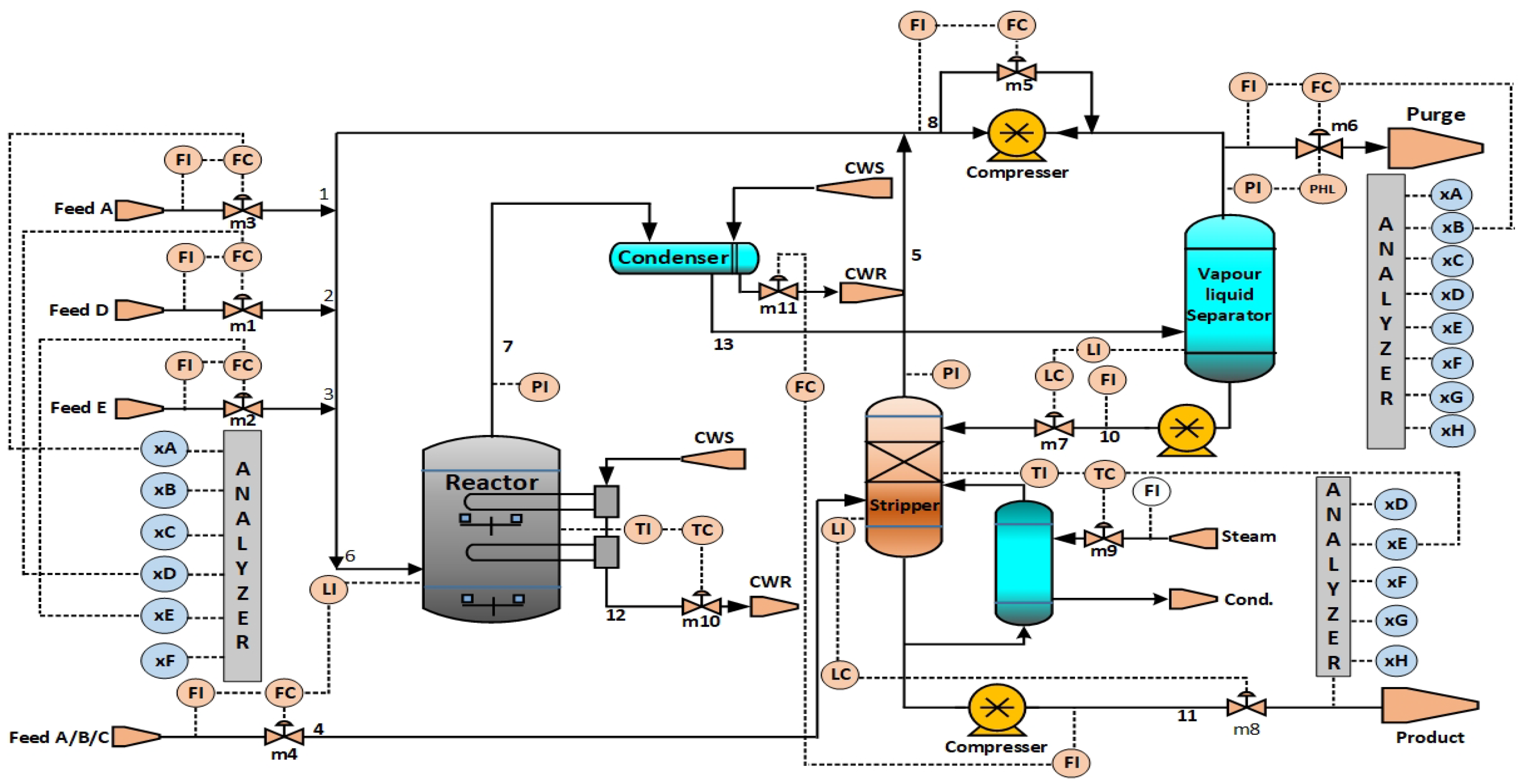
This section presents the results of applying the proposed methodology to two prominent benchmarks: the Tennessee Eastman (TE) process and Benchmark Simulation 1 (BSM1). The effectiveness of the monitoring methodology is evaluated using widely recognized metrics for process monitoring performance: missed alarm rate (MAR), false alarm rate (FAR), error detection delay, and number of errors detected. Error detection technology intends to be rapid in identifying faults, sensitive to all potential process errors, and robust to data variations. To evaluate the resilience of each statistic, the false alarm rate for the test set under normal operating parameters has been determined and compared to the statistical significance level that sets the threshold. The sensitivity level of the missing detection rate was evaluated using the missing detection rate, and the speed of implementation of measures was measured by determining the delay. The Missed Alarm Rate (MAR) shows the proportion of erroneous data that are mistakenly identified as error-free data. Specifically, the number of incomplete data samples that do not exceed the control limits is divided by the total number of incomplete data samples to determine the MAR.

5.1. Case Study 1

Tennessee Eastman Process (TE) The Tennessee Eastman (TE) process is a well-known simulation model of a real industrial chemical process. This approach applies to many other control-related problems and is extremely relevant for research in process control technology [40]. The five main components of the TE process are shown in Figure 1 flow diagram: a reactor, a product condenser, a vapor-liquid separator, a recycle compressor, and a product stripper. Together, these components enable reactor, separation, and recycling processes inside a closed-loop control structure that spans the entire process.

TE Dataset Details

This simulation process can replicate normal operating conditions and 21 different failure scenarios, generating simulated data at 3-min intervals. For each scenario, whether normal or faulty, two data sets are produced: training data sets and testing data sets. Training data sets are used to develop statistical predictive models while testing data sets are used to evaluate the accuracy of these models. Specifically, the training data set for the normal case contains 500 samples, while each faulty case data set contains 480 samples. Each test data set, which is applied to normal and faulty conditions, contains 960 samples. It is worth noting that the training set samples were obtained after 25 h of simulation with defects. There is no error mode at the beginning of the simulation, and the error occurs when the simulation time is 1 h. However, the observational data collected after the error was introduced amounted to only 480 observations. Samples of the test set with errors were obtained during a 48-h simulation. In fault-related cases, the fault appears 8 h after the TE process has begun. As a result, the first 160 samples in these faulty conditions represent normal operation, but the remaining 800 examples demonstrate fault situations that should be identified. Each observation sample in these datasets has 52 variables, 22 process measurement variables, 19 component measurement variables, and 12 control variables. The TE process is used as a benchmark for industrial process control and monitoring research. It reflects a realistic chemical plant context, making it a widely used model for comparing the effectiveness of various procedures. The process produces two products from four reactants, including an inert component and a by-product, giving a total of eight components labeled A, B, C, D, E, F, G, and H. Among the 52 measurements obtained from the procedure, 41 are process variables and 11 are controlled variables. Initially, Downs and Vogel identified 20 process flaws, with an additional valve fault inserted in a later study [41], as shown in

Table 1. Descriptions of Faults in the Tennessee Eastman (TE) Process.

Fault ID	Description
IDV0	Normal operation
IDV1	Variations in A/C feed ratio with constant B composition
IDV2	Changes in B composition with a constant A/C ratio
IDV4	Fluctuations in reactor cooling water inlet temperature
IDV5	Variations in condenser cooling water inlet temperature
IDV6	Loss of A feed (stream 1)
IDV7	Pressure drop in C header, leading to reduced availability (stream 4)
IDV8	Variations in feed composition of A, B, and C (stream 4)
IDV10	Changes in C feed temperature (stream 4)
IDV11	Reactor cooling water inlet temperature variations
IDV12	Condenser cooling water inlet temperature variations
IDV13	Changes in reaction kinetics
IDV14	Issues with the reactor cooling water valve
IDV16	Unknown fault type
IDV17	Unknown fault type
IDV18	Unknown fault type
IDV19	Unknown fault type
IDV20	Unknown fault type

.

Tennessee Eastman Process fault 5 is a step change in the cooling water inlet temperature to the condenser. The problem begins at the fluctuation in the feed stream, which causes heat transfer performance, product quality, and stability of operations to be compromised. Effective monitoring and detection of this problem are critical for ensuring safe and efficient operation. This study presents the MAR (Missed alarm rate) and FAR (False alarm rate) values for various metrics, including $T^2$, $S^2$, and SPE, explained through various approaches such as SFA (slow feature analysis), KSFA (Kernel slow feature analysis), DSFA (Dynamic Slow feature analysis), and PCA (Principal Component Analysis).

The MAR of $T^2$ statistics under both Slow feature analysis (SFA) and Principal Component Analysis (PCA) show no deviation during the monitoring phase when the process is under normal operational conditions. The significant FAR ($T^2$) in SFA and even higher in PCA (18.125 (SFA), 100 (PCA)) suggests strong sensitivity to fault detection, indicating substantial deviation when the fault is present as shown in

Table 2. False Alarm Rate (FAR) and Missed Alarm Rate (MAR) of TE for all monitoring methods (%).

Metric	SFA	KSFA	DSFA	PCA
${\mathrm{MAR}}_{T^2}$	0	-	-	0
${\mathrm{FAR}}_{T^2}$	18.125	-	-	100
${\mathrm{MAR}}_{S^2}$	62.907	1.961	-	0
${\mathrm{FAR}}_{S^2}$	10	1.389	-	99.375
${\mathrm{MAR}}_{T_e^2}$	0	-	-	-
${\mathrm{FAR}}_{T_e^2}$	10.625	-	-	-
${\mathrm{MAR}}_{S_e^2}$	93.484	-	-	-
${\mathrm{FAR}}_{S_e^2}$	3.75	-	-	-
${\mathrm{MAR}}_{\mathrm{SPE}}$	-	1.961	-	-
${\mathrm{FAR}}_{\mathrm{SPE}}$	-	2.778	-	-
${\mathrm{MAR}}_D$	-	-	76.441	-
${\mathrm{FAR}}_D$	-	-	0	-

.

The MAR of $S^2$ statistics for SFA, KSFA, PCA: 62.90727 (SFA), 1.960784 (KSFA), 0 (PCA)—High values in SFA denote significant monitoring residuals, suggesting notable changes in the process under normal operation. KSFA shows moderate residuals, while PCA shows no significant deviation.

MAR $T_e^2$ (SFA): 0—No deviations are noted, consistent with normal operational stability. While FAR$T_e^2$ (SFA): 10.625—A significant increase in FAR reflects the fault’s impact, indicating this metric’s effectiveness in fault detection.

MAR$S_e^2$ (SFA): 93.48371—This high value indicates substantial residuals in the monitoring phase, suggesting notable variance even under normal conditions. FAR$S_e^2$ (SFA): 3.75—A relatively lower FAR indicates sensitivity to detecting the specific fault without large false positives.

MAR_SPE (KSFA): 1.960784 (SFA)—Low KSFA values suggest minimal residuals under normal operations, whereas DSFA shows substantial residuals. FAR_SPE (KSFA): 2.777778 (SFA), KSFA indicates moderate fault detection capability, denoting precise fault detection.

MAR_D (DSFA): 76.4411—High monitoring residuals in the DSFA approach indicate sensitivity to deviations during normal operations. FAR_D (DSFA): 0—No false alarms during fault detection, suggesting excellent sensitivity and precision.

Based on the MAR and FAR values, Dynamic Slow Feature Analysis (DSFA) appears to be the best method. It has high MAR values and very low FAR values across different statistics, indicating a strong fault detection capability with minimal false alarms.

Slow Feature Analysis (SFA) is applied to the TE data set to monitor process performance. The $T^2$ and $S^2$ statistics, as per SFA, are illustrated in Figure 2a. From the $T^2$ plot, it is evident that the $T^2$ statistic starts to escalate significantly after around 200 samples, surpassing the control limit line (depicted in red), indicating a shift in process behavior and potential anomaly detection. The $S^2$ statistic also shows deviations around the same region, providing additional corroborative evidence of the process change. The peaks observed in the $S^2$ plot reinforce the effectiveness of SFA in capturing significant slow temporal features associated with the process changes.

Figure 2b demonstrates the results of applying Kernel Slow Feature Analysis (KSFA) to the same data set. Nonlinear dependencies in the data can be captured by KSFA, in contrast to linear SFA. It can be observed that the $S^2$ values exhibit sharp peaks, particularly around sample indices 200 and 400, which supports the existence of disturbances during these time intervals. Significant departures from control limits are also identified using the SPE statistic, which offers reliable identification of outliers in process data and underlying nonlinear dynamics.

The outcomes of dynamic slow feature analysis (DSFA), which enhances process monitoring by merging temporal dynamics and SFA, are displayed in Figure 2c. Process volatility is clearly indicated by the D statistic, which has a notable peak around the first 200 samples. When compared to conventional SFA and KSFA, DSFA successfully captures dynamic features that signify process violations and offers a richer representation of temporal relationships.

Principal component analysis (PCA), as illustrated in Figure 2d, was also used to assess the effectiveness of SFA, KSFA, and DSFA. A big peak first appears on the $T^2$ PCA plot, but anomalies are continuously missed after that. Comparatively to other methods analyzed, the SPE statistic also records initial growth but is less responsive to later aberrations. The inability of PCA to identify process problems quickly enough illustrates the drawbacks of conventional linear procedures in comparison to more sophisticated approaches like SFA, KSFA, and DSFA.

5.2. Discussion

The comparative analysis demonstrates that although traditional PCA has its uses, it is not able to reliably identify abnormalities in intricate, nonlinear data. Although SFA performs better, it could have challenges capturing very non-linear correlations. By utilizing updated techniques, KSFA closes this gap and improves anomaly detection. On the other hand, DSFA seems to be the most potent fire-related temporal dynamic that more fully captures performance variations. Overall, KSFA and DSFA have good anomaly detection abilities for complicated datasets like TE, with DSFA excelling at recognizing critical time dependencies in dynamic process contexts. These findings emphasize the significance of sophisticated feature analysis techniques in capturing overall process behavior for improved monitoring and error identification.

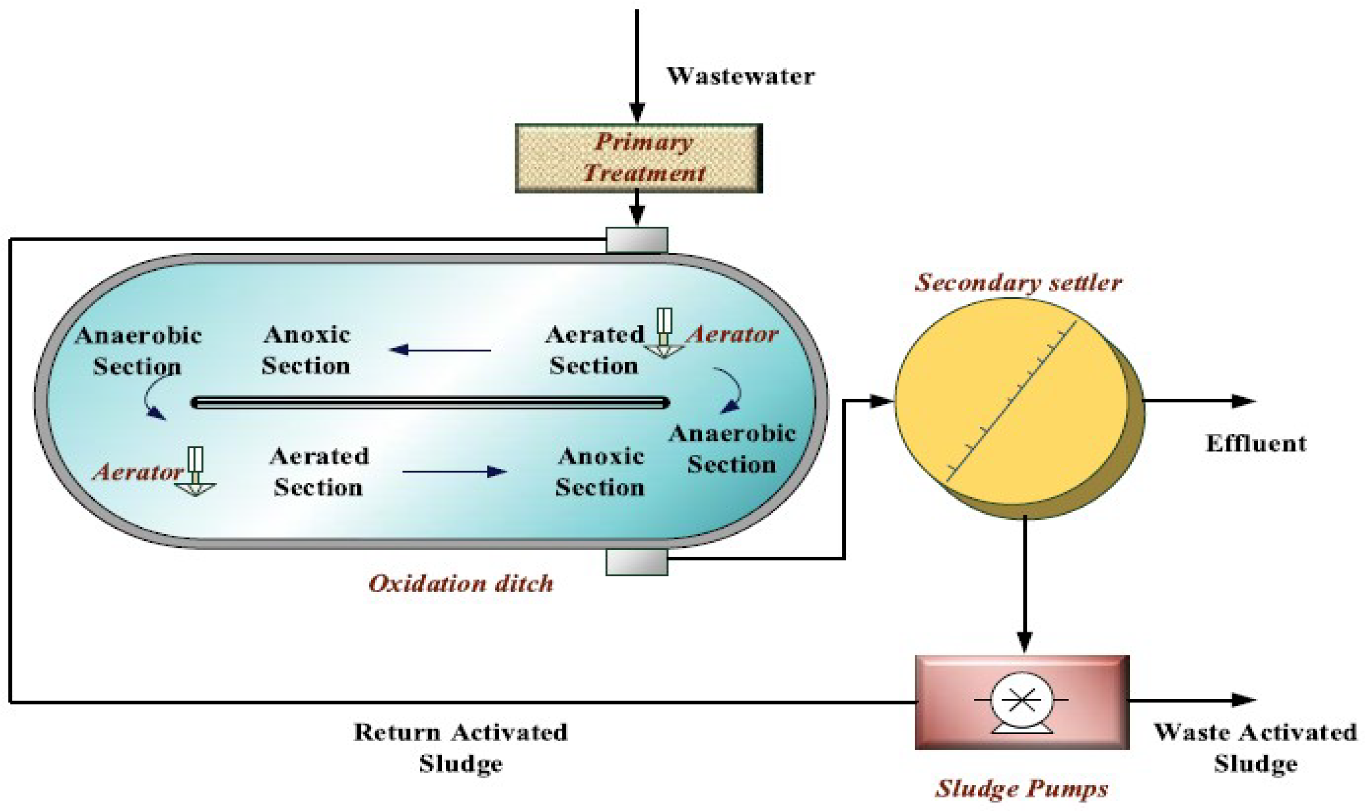
5.3. Case Study 2: Benchmark Simulation 1 (BSM 1)

Wastewater treatment plants (WWTPs) are complicated biochemical systems that exhibit non-linear dynamics and non-Gaussian data distribution. These challenges arise from interactions between microbial activity, ambient noise, and process factors [42]. Nonlinearities in wastewater treatment plants come from the interconnectedness of process variables, which causes complicated changes in the system’s behavior. Furthermore, the impact of environmental influences on closed-loop monitoring systems creates a non-Gaussian pattern in the process data. The non-Gaussian nature of wastewater treatment data complicates feature extraction by making it difficult to appropriately describe the data underlying the derived features. As a result, it is critical to look into techniques that lessen the non-Gaussian effect while also improving feature extraction. Furthermore, wastewater treatment plants are multi-stage, which means that distinct biochemical reactions occur in every phase of treatment. This makes it challenging to employ a consistent modeling method to investigate the key properties associated with each phase. The multi-phase, non-Gaussian, and non-linear properties of wastewater treatment plants present substantial problems for data-driven process monitoring. To address these problems, effective monitoring models must be developed that can properly identify and diagnose system faults [43].

Benchmark Simulation Model 1 (BSM1) is a complete simulation environment. It was created by the International Water Association (IWA) and the COST Action Working Groups 682 and 624 [44,45]. The platform mimics the action of activated sludge, which removes carbon (C) and organic matter including nitrogen (N), phosphorous (P), and other associated components from wastewater nitrification and denitrification processes. This activity removes insoluble and biodegradable materials using flocculent bacteria. In the secondary treatment tank, the purified water is eventually discharged into the receiver medium.

The BSM1 structure, shown in Figure 3, consists of activated sludge model no. 1 (ASM1) with a capacity of 5999 m³ and a secondary settling tank with a capacity of 6000 m³. ASM1 consists of five reaction tanks: the first two tanks (each 1000 m³) are anaerobic, followed by three aerobic tanks (each 1333 m³) [46]. Wastewater from the fifth reaction tank is partially returned to the first tank for internal recycling, while the remaining wastewater goes to the secondary settling tank. The secondary settling tank separates suspended particles and facilitates the separation of solids and liquids. Clean sewage is discharged from the upper layers and sludge from the lower layers is returned to ASM1 via the external loop.

BSM1 can simulate dry, rainy and stormy conditions in a wastewater treatment plant (WWTP) over 14 days, collecting sensor data every 15 min for a total of 1344 samples. The modeled type of defect is toxic shock, which affects the metabolism of heterotrophic bacteria under the influence of toxic substances present in the fluid. The nature of the fault course is characterized by non-linear attributes. These are visually determined by sharp early spikes in the plots, followed by stabilization or variations. This designates swift fluctuations in the system rather than gradual, linear increases. This error is simulated by adjusting the growth rate of heterotrophic bacteria. In the toxicity error scenario, it was presented in sample #845, with the first 700 samples used for training and the remaining 644 samples used for testing [47,48].

Table 3. The FAR and MAR of BSM1 for all monitoring methods (%).

Metric	SFA	KSFA	DSFA	PCA
MAR_T2	92.07082	NA	NA	27.30769
FAR_T2	0	NA	NA	70.45455
MAR_S2	26.097	54.92308	NA	99.61538
FAR_S2	65.90909	2.272727	NA	0
MAR_T2e	86.98999	NA	NA	NA
FAR_T2e	2.272727	NA	NA	NA
MAR_S2e	97.5366	NA	NA	NA
FAR_S2e	2.272727	NA	NA	NA
MAR_SPE	NA	80	NA	NA
FAR_SPE	NA	0	NA	NA
MAR_D	NA	NA	61.89376	NA
FAR_D	NA	NA	0	NA

presents a comparative analysis of different monitoring methods used in the BSM1 Benchmark simulation process for detecting toxicity faults. The methods compared include Slow Feature Analysis (SFA), Kernel Slow Feature Analysis (KSFA), Dynamic Slow Feature Analysis (DSFA), and Principal Component Analysis (PCA). Various metrics are used to evaluate the performance of these methods, including Missed Alarm Rate (MAR) and False Alarm Rate (FAR) for different statistics ($T^2$, $S^2$, SPE, and D).

6. Discussion

MAR_$T^2$ of SFA shows a high MAR of 92.07082, indicating a significant number of missed alarms. PCA has a lower MAR of 27.30769 compared to SFA, suggesting better fault detection capability. FAR_$T^2$ for both SFA and PCA illustrate divergent trends with SFA having no false alarms and PCA showing a high FAR of 70.45455. This implies SFA’s conservative approach results in no false positives, whereas PCA may generate numerous false alarms.

MAR_D for DSFA has the highest MAR of 61.89376, indicating many missed faults. KSFA shows moderate MAR (54.92308) and SFA has the lowest amongst these (26.097), suggesting varying effectiveness across methods.

FAR_$S^2$ for SFA has a fairly high FAR at 65.90909, indicating many false positives. KSFA shows much fewer false alarms (2.272727), and DSFA demonstrates no false alarms, indicating higher reliability.

MAR_$T_e^2$ for SFA yields a MAR of 86.98999, indicating substantial missed alarms. MAR_$S_e^2$ for SFA has a very high MAR of 97.5366, implying numerous missed alarms. FAR_$S_e^2$ SFA again shows minimal false alarms with a FAR of 2.272727.

MAR_SPE for KSFA reports a MAR of 80, suggesting a significant number of missed alarms while FAR_SPE for KSFA shows no false alarms under this metric. MAR_D for DSFA reports considerable missed alarms with MAR at 61.89376 while FAR_D for DSFA shows great precision with no false alarms reported.

Based on the MAR and FAR values, Dynamic Slow Feature Analysis (DSFA) appears to be the most effective method for fault detection. It demonstrates high MAR values and low FARs across different metrics, indicating a strong capability to detect faults with minimal false positives. In particular, DSFA performance is highlighted by its excellent precision noted by zero false alarms in FAR_D metrics, suggesting a robust and reliable monitoring solution for the BSM1 Benchmark simulation process.

Performance Evaluation of Monitoring Methods

Figure 4 evaluates the performance of Slow Feature Analysis (SFA), Kernel Slow Feature Analysis (KSFA), Dynamic Slow Feature Analysis (DSFA), and Principal Component Analysis (PCA) for detecting toxicity faults in the BSM1 dataset. The output graphs of each method are displayed in Figure 1, and a detailed comparison is provided below.

Figure 4a displays the performance of SFA in monitoring the toxicity fault. The statistical indices used include T2 and S2. T2 and S2 metrics show several significant spikes, indicating the moments of detected faults. The T2 and T2e charts indicate numerous out-of-control events by crossing the threshold more prominently than the S2 statistics. False positives appear to be fewer in the S2 charts.

Figure 4b shows the KSFA results with the S2 and SPE statistics. KSFA demonstrates a clear signal for fault detection. The S2 statistic shows multiple sharp peaks precisely corresponding to the fault injection points. The SPE statistic effectively identifies the fault occurrence with significant peaks, indicating KSFA’s strong sensitivity to the changes in data due to faults.

Figure 4c features the DSFA output using the D statistic. The D statistic exhibits increased variability and several prominent spikes after fault occurrences. The DSFA method effectively highlights the dynamism in the system due to the faults, as indicated by the increasing D values in the latter samples where the faults are more severe or frequent.

Figure 4d provides the PCA results through the $T^2$ and SPE statistics. PCA $T^2$ statistic prominently detects faults with sharp, significant spikes, surpassing the set threshold predominantly towards the latter samples. The SPE statistic also indicates fault detection, showcasing several spikes. However, the magnitude of these spikes is substantially lower compared to SFA and DSFA, suggesting PCA’s relatively lower sensitivity in the presence of nonlinearities.

KSFA and DSFA show enhanced sensitivity to fault conditions, detecting multiple peaks with higher intensity compared to standard SFA and PCA, suggesting better fault detection capacity. SFA efficiently identifies faults with fewer false positives in $S^2$ metrics but shows high false alarms in $T^2$ statistics. On the other hand, DSFA is dynamic approach captures fault progression effectively. KSFA and DSFA, incorporating non-linear and dynamic components, are computationally more intensive compared to linear methods like PCA and SFA. KSFA stands out in capturing non-linear relationships, whereas DSFA is beneficial in dynamic systems handling changes over time.

In conclusion, while all approaches are useful for fault detection, KSFA and DSFA have higher fault sensitivity and isolation abilities for BSM 1 toxicity fault detection, particularly in complicated, non-linear, and dynamic data circumstances. More research could focus on merging or enhancing these algorithms to improve outcomes in real-world fault detection scenarios.

The advent of Kernel Slow Feature Analysis (KSFA) and Dynamic Slow Feature Analysis (DSFA) represents substantial advances in fault detection, displaying increased sensitivity and efficient classification capabilities over older and standard methods, such as SFA and PCA. Also, KSFA can successfully capture non-linear relationships, whereas DSFA excels at handling dynamic system changes and achieves high precision with 0 percent false alarms in measurements, like FAR_$S^2$ and FAR_D, suggesting remarkable fault detection performance. These methods are particularly useful in scenarios involving complex, non-linear, and dynamic data, as indicated by their improved performance in the presented measures, which significantly improve fault detection accuracy and robustness.

Notice that the results presented in this paper are derived from simulation data, which offer a controlled and replicable environment to evaluate fault detection methods comprehensively. The real-world data may exhibit greater complexity and variability, thus the use of simulations is crucial for thoroughly testing and refining our models under a wide range of conditions. This approach allows us to isolate specific variables and assess the theoretical performance limits of our methods, providing valuable insights before applying them to any real-world scenarios. Additionally, our model for the current assessment is able to explore an area that has not been extensively explored recently. This makes our approach particularly valuable for advancing research in fault detection within processing plants. By applying our model, we provide new insights and tools that enhance the accuracy and effectiveness of fault detection, positioning it as a leading method in this field.

7. Real World Wastewater Treatment Plant

Wastewater treatment plants (WWTPs) are intricate systems designed to manage large volumes of municipal wastewater. The fundamental nitrification and denitrification processes in the treatment tanks contribute to complex time-series relationships among various operational data. When the sampling interval is short, the dynamic behaviors of the monitored variables can become particularly pronounced. The full-scale WWTP in Beijing, China, which is the focus of this case study, uses the oxidation ditch (OD) technology primarily to treat urban wastewater is shown in Figure 5. The longer solids retention time (SRT) of the OD process, an improved activated sludge process, ensures effective nitrogen removal. As illustrated in the schematic diagram (Figure 5), the plant handles an average influent flow of approximately 170,000 m³ per day and maintains a hydraulic retention time (HRT) of 16.5 h [49].

The SRT is controlled by selectively eliminating sludge from the secondary sedimentation tank between 15 and 22 days. The plant has encountered filamentous sludge bulking, a problem that lasted for roughly six months, despite a low chemical oxygen demand (COD) loading rate of less than 0.25 kg COD/kg MLSS/day. Throughout this time, the influent characteristics, operating conditions, and the development of the sludge volume index (SVI) were meticulously recorded. In WWTPs, especially those that use the oxidation ditch process, filamentous sludge bulking often arises from environmental factors such as temperature changes during seasonal transitions. Nevertheless, the lack of available monitoring equipment and sensors renders it challenging to locate this problem in real-time, so choosing the right statistical process monitoring technique is critical for prompt abnormality identification. Due to practical and financial limitations, it is not feasible to install monitoring sensors throughout the entire plant. Instead, this study focuses on eight readily obtainable monitoring variables from the outlet of the secondary sedimentation tank (as detailed in

Table 4. The FAR and MAR of Beijing Plant for all monitoring methods (%).

	SFA				KSFA		DSFA	PCA
	${\mathit{T}}^{\mathbf{2}}$	${\mathit{S}}^{\mathbf{2}}$	${\mathit{T}}_{\mathit{e}}^{\mathbf{2}}$	${\mathit{S}}_{\mathit{e}}^{\mathbf{2}}$	${\mathit{S}}^{\mathbf{2}}$	SPE	$\mathit{D}$	${\mathit{T}}^{\mathbf{2}}$	SPE
MAR	5.421	38.55	0	0	27.54	2	53.01	3.5	16.7
FAR	0	0	0	0	2	6	0	28.8	0

). The data was collected as daily mean values from multiple samples, resulting in a total of 213 samples for analysis.

Initial analysis concentrated on the first 45 samples, which were collected under stable operating conditions with SVI values below 150 g/mL. During the period between the 46th and 106th samples, the SVI exhibited oscillatory behavior around the control limit, indicating the potential for incipient faults. Following this phase, a significant increase in SVI was observed starting on day 107, signaling the onset of notable sludge bulking. Early detection of such incipient faults can facilitate timely adjustments to system parameters, helping to avert severe sludge bulking problems. Thus, the first 45 samples were utilized for offline training of the monitoring methods. Subsequently, all 213 samples were employed as a test data set to enhance online monitoring capabilities [47]. This case study highlights the importance of effective monitoring methods in managing filamentous sludge bulking within large-scale wastewater treatment facilities Operators can better predict and manage operational issues, ensuring the ongoing stability and efficacy of treatment operations, by using statistical process monitoring approaches and focusing on easily accessible data. The results of this study demonstrate the significance of ongoing innovation in monitoring procedures, which will be essential for wastewater treatment plants to continue operating efficiently in the future.

The experimental evaluation of the fault detection approach using Slow Feature Analysis (SFA) demonstrates varied efficacy as reflected in the T² and S² statistics and their enhanced versions, T²e and S²e. The T² measure recorded a Miss Alarm Rate (MAR) of 5.4 and a False Alarm Rate (FAR) of 0 as shown in Table 4, signifying strong detection accuracy with no false positives detected. In contrast, the S² measure showed a greater MAR of 38.6 but similarly achieved a FAR of 0, indicating a trade-off between sensitivity and specificity.

The enhanced statistics, T²e and S²e, improved drastically, with both registering perfect scores with MAR and FAR at 0, demonstrating that the enhancement methods significantly enhance detection effectiveness while completely eliminating false alarms. Analyzing the time-series plots supports these conclusions: T² exhibited moderate fluctuations punctuated by notable peaks, while T²e maintained a stable path. The S² measure saw pronounced spikes around sample 100, whereas S²e stayed consistently stable as shown in Figure 6.

KSFA’s performance was assessed using the S² and Squared Prediction Error (SPE) statistics. For the S² statistic, a Missing Alarm Rate (MAR) of 27.54 and a False Alarm Rate (FAR) of 2.22 were recorded, indicating a balance between detection sensitivity and specificity. The SPE statistic demonstrated a considerably lower MAR of 2.99 but a slightly increased FAR of 6.67. These results highlight the complementary nature of S² and SPE in KSFA, where their combined use can enhance fault detection by balancing sensitivity and specificity. The monitoring charts reveal that the S² statistic captures pronounced changes, particularly post-sample 150, while the SPE statistic remains stable but shows significant deviations around sample 100. The low FAR values for both statistics confirm effective fault detection without excessive false positives, underscoring KSFA’s capability to monitor process deviations robustly. DSFA exhibited distinct results with the D statistic, achieving a zero FAR, indicating impeccable specificity without false alarms. However, the MAR stood at 53.01, suggesting lower sensitivity in detecting faults. This significant trade-off points to DSFA’s strength in eliminating false positives while indicating potential improvements needed in sensitivity for detecting subtle anomalies.

The monitoring graph depicts the D statistic’s evolution, transitioning from stable normal operation to detecting persistent fault conditions starting around sample 75. Despite the high MAR, DSFA’s ability to maintain elevated D values during fault conditions attests to its robustness in continuous monitoring systems. PCA presented a nuanced trade-off between T² and SPE statistics. T² MAR of 3.6 suggests good sensitivity; however, a high FAR of 28.9 indicates frequent false alarms. Conversely, SPE demonstrated zero false alarms but higher MAR, underscoring its conservative detection approach. PCA’s dual-statistic approach emphasizes the benefits of using both sensitivity and specificity-focused metrics for effective monitoring. In summary, KSFA and DSFA offer distinct advantages for fault detection, with KSFA providing a balanced detection capability and DSFA excelling in specificity. These methodologies, when compared to SFA and PCA, suggest potential for integrative approaches that harness the strengths of each method for optimized monitoring in industrial applications.

8. Conclusions and Future Work

This comparative study of fault detection algorithms examines the strengths and shortcomings of SFA, KSFA, DSFA, and PCA when applied to the TE and BSM 1 datasets. Kernel Slow Feature Analysis (KSFA) and Dynamic Slow Feature Analysis (DSFA) can increase the sensitivity of fault detection and isolation. KSFA excels at capturing non-linear dependencies, whereas the incorporation of time dynamics in DSFA enables effective monitoring of dynamic process changes. Both KSFA and DSFA have outstanding fault detection and isolation capabilities in terms of FAR and MAR, making them appropriate for complex and dynamic operating settings. Based on the findings of this work, future research can concentrate on many key areas for improving error detection methods. By combining the benefits of KSFA and DSFA, a hybrid model based on nonlinear and dynamic feature extraction can give improved sensitivity and reliability for fault identification. Investigate the use of real-time KSFA and DSFA in an industrial setting to maximize computational economy without sacrificing fault detection performance. Investigate scalable versions of these technologies to handle the huge data flows found in modern industrial environments. These technologies have been enhanced not only with the ability to detect anomalies but also to diagnose the underlying cause of those anomalies. Deep learning approaches, when combined with KSFA and DSFA, can capture more complicated and subtle patterns in data, improving error detection and prediction skills. Our simulations could favor the future research exploration of these methods using more real-world data, yet it is noticeable that our findings provide a robust foundation to advance the understanding and development of fault detection capabilities.

References

1. Li, W.; Huang, R.; Li, J.; Liao, Y.; Chen, Z.; He, G.; Yan, R.; Gryllias, K. A perspective survey on deep transfer learning for fault diagnosis in industrial scenarios: Theories, applications and challenges. Mech. Syst. Signal Process. 2022, 167, 108487. [Google Scholar] [CrossRef]
2. Wang, J.; Ye, L.; Gao, R.X.; Li, C.; Zhang, L. Digital Twin for rotating machinery fault diagnosis in smart manufacturing. Int. J. Prod. Res. 2019, 57, 3920–3934. [Google Scholar] [CrossRef]
3. Wan, J.; Li, X.; Dai, H.N.; Kusiak, A.; Martinez-Garcia, M.; Li, D. Artificial-intelligence-driven customized manufacturing factory: Key technologies, applications, and challenges. Proc. IEEE 2020, 109, 377–398. [Google Scholar] [CrossRef]
4. Yan, R.; Gao, R.X.; Chen, X. Wavelets for fault diagnosis of rotary machines: A review with applications. Signal Process. 2014, 96, 1–15. [Google Scholar] [CrossRef]
5. Wang, R.; Zhan, X.; Bai, H.; Dong, E.; Cheng, Z.; Jia, X. A Review of Fault Diagnosis Methods for Rotating Machinery Using Infrared Thermography. Micromachines 2022, 13, 1644. [Google Scholar] [CrossRef] [PubMed]
6. Lei, Y.; Li, N.; Guo, L.; Li, N.; Yan, T.; Lin, J. Machinery health prognostics: A systematic review from data acquisition to RUL prediction. Mech. Syst. Signal Process. 2018, 104, 799–834. [Google Scholar] [CrossRef]
7. Huang, R.; Li, J.; Wang, S.; Li, G.; Li, W. A robust weight-shared capsule network for intelligent machinery fault diagnosis. IEEE Trans. Ind. Inform. 2020, 16, 6466–6475. [Google Scholar] [CrossRef]
8. Liu, D.; Song, Y.; Li, L.; Liao, H.; Peng, Y. On-line life cycle health assessment for lithium-ion battery in electric vehicles. J. Clean. Prod. 2018, 199, 1050–1065. [Google Scholar] [CrossRef]
9. Wang, K.; Zhou, W.; Mo, Y.; Yuan, X.; Wang, Y.; Yang, C. New mode cold start monitoring in industrial processes: A solution of spatial–temporal feature transfer. Knowl.-Based Syst. 2022, 248, 108851. [Google Scholar] [CrossRef]
10. Fang, R.; Wang, K.; Li, J.; Yuan, X.; Wang, Y. Unsupervised domain adversarial network for few-sample fault detection in industrial processes. Adv. Eng. Inform. 2024, 61, 102684. [Google Scholar] [CrossRef]
11. Peres, F.A.P.; Peres, T.N.; Fogliatto, F.S.; Anzanello, M.J. Fault detection in batch processes through variable selection integrated to multiway principal component analysis. J. Process Control 2019, 80, 223–234. [Google Scholar] [CrossRef]
12. Zhang, J.; Chen, M.; Hong, X. Nonlinear process monitoring using a mixture of probabilistic PCA with clusterings. Neurocomputing 2021, 458, 319–326. [Google Scholar] [CrossRef]
13. Huang, J.; Yang, X.; Shardt, Y.A.; Yan, X. Sparse modeling and monitoring for industrial processes using sparse, distributed principal component analysis. J. Taiwan Inst. Chem. Eng. 2021, 122, 14–22. [Google Scholar] [CrossRef]
14. Liu, Y.; Pan, Y.; Sun, Z.; Huang, D. Statistical monitoring of wastewater treatment plants using variational Bayesian PCA. Ind. Eng. Chem. Res. 2014, 53, 3272–3282. [Google Scholar] [CrossRef]
15. Yang, Y.H.; Chen, Y.L.; Chen, X.B.; Qin, S.K. Multivariate statistical process monitoring and fault diagnosis based on an integration method of PCA-ICA and CSM. Appl. Mech. Mater. 2011, 84, 110–114. [Google Scholar] [CrossRef]
16. Kini, K.R.; Madakyaru, M. Improved process monitoring scheme using multi-scale independent component analysis. Arab. J. Sci. Eng. 2022, 47, 5985–6000. [Google Scholar] [CrossRef]
17. Harkat, M.F.; Mansouri, M.; Nounou, M.N.; Nounou, H.N. Fault detection of uncertain chemical processes using interval partial least squares-based generalized likelihood ratio test. Inf. Sci. 2019, 490, 265–284. [Google Scholar]
18. Zhang, K.; Hao, H.; Chen, Z.; Ding, S.X.; Peng, K. A comparison and evaluation of key performance indicator-based multivariate statistics process monitoring approaches. J. Process Control 2015, 33, 112–126. [Google Scholar] [CrossRef]
19. Liu, H.; Yang, J.; Zhang, Y.; Yang, C. Monitoring of wastewater treatment processes using dynamic concurrent kernel partial least squares. Process Saf. Environ. Prot. 2021, 147, 274–282. [Google Scholar] [CrossRef]
20. Yao, L.; Shao, W.; Ge, Z. Hierarchical quality monitoring for large-scale industrial plants with big process data. IEEE Trans. Neural Netw. Learn. Syst. 2019, 32, 3330–3341. [Google Scholar] [CrossRef]
21. Zou, W.; Xia, Y.; Li, H. Fault diagnosis of Tennessee—Eastman process using orthogonal incremental extreme learning machine based on driving amount. IEEE Trans. Cybern. 2018, 48, 3403–3410. [Google Scholar] [CrossRef] [PubMed]
22. Qian, Q.; Qin, Y.; Wang, Y.; Liu, F. A new deep transfer learning network based on convolutional auto-encoder for mechanical fault diagnosis. Measurement 2021, 178, 109352. [Google Scholar] [CrossRef]
23. Cai, L.; Tian, X.; Chen, S. Monitoring nonlinear and non-Gaussian processes using Gaussian mixture model-based weighted kernel independent component analysis. IEEE Trans. Neural Netw. Learn. Syst. 2017, 28, 122–135. [Google Scholar] [CrossRef] [PubMed]
24. Lee, J.-M.; Yoo, C.K.; Choi, S.W.; Vanrolleghem, P.A.; Lee, I.-B. Nonlinear process monitoring using kernel principal component analysis. Chem. Eng. Sci. 2004, 59, 223–234. [Google Scholar] [CrossRef]
25. Zhang, Q.; Li, P.; Lang, X.; Miao, A. Improved dynamic kernel principal component analysis for fault detection. Measurement 2020, 158, 107738. [Google Scholar] [CrossRef]
26. Dong, Q. Implementing deep learning for comprehensive aircraft icing and actuator/sensor fault detection/identification. Eng. Appl. Artif. Intell. 2019, 83, 28–44. [Google Scholar] [CrossRef]
27. Yu, W.; Zhao, C. Robust monitoring and fault isolation of nonlinear industrial processes using denoising autoencoder and elastic net. IEEE Trans. Control Syst. Technol. 2020, 28, 1083–1091. [Google Scholar] [CrossRef]
28. Xiao, Y.C.; Wang, H.G.; Zhang, L.; Xu, W.L. Two methods of selecting Gaussian kernel parameters for one-class SVM and their application to fault detection. Knowl.-Based Syst. 2014, 59, 75–84. [Google Scholar] [CrossRef]
29. Zhang, S.; Zhao, C. Slow-feature-analysis-based batch process monitoring with comprehensive interpretation of operation condition deviation and dynamic anomaly. IEEE Trans. Ind. Electron. 2018, 66, 3773–3783. [Google Scholar] [CrossRef]
30. Guo, F.; Shang, C.; Huang, B.; Wang, K.; Yang, F.; Huang, D. Monitoring of operating point and process dynamics via probabilistic slow feature analysis. Chemom. Intell. Lab. Syst. 2016, 151, 115–125. [Google Scholar] [CrossRef]
31. Shang, C.; Huang, B.; Yang, F.; Huang, D. Slow feature analysis for monitoring and diagnosis of control performance. J. Process Control 2016, 39, 21–34. [Google Scholar] [CrossRef]
32. Pilario, K.E.; Shafiee, M.; Cao, Y.; Lao, L.; Yang, S.H. A review of kernel methods for feature extraction in nonlinear process monitoring. Processes 2019, 8, 24. [Google Scholar] [CrossRef]
33. Song, P.; Zhao, C. Slow down to go better: A survey on slow feature analysis. IEEE Trans. Neural Netw. Learn. Syst. 2022, 35, 3416–3436. [Google Scholar] [CrossRef] [PubMed]
34. Melo, A.; Câmara, M.M.; Pinto, J.C. Data-Driven Process Monitoring and Fault Diagnosis: A Comprehensive Survey. Processes 2024, 12, 251. [Google Scholar] [CrossRef]
35. Zhang, N.; Tian, X.; Cai, L.; Deng, X. Process fault detection based on dynamic kernel slow feature analysis. Comput. Electr. Eng. 2015, 41, 9–17. [Google Scholar] [CrossRef]
36. Fang, M. Hierarchical Monitoring and Probabilistic Graphical Model Based Fault Detection and Diagnosis. Ph.D Thesis, Department of Chemical and Materials Engineering, University of Alberta, Edmond, AB, USA, 2020. [Google Scholar]
37. Bounoua, W.; Aftab, M.F. Improved extended empirical wavelet transform for accurate multivariate oscillation detection and characterisation in plant-wide industrial control loops. J. Process Control. 2024, 138, 103226. [Google Scholar] [CrossRef]
38. Liu, S.; Lei, F.; Zhao, D.; Liu, Q. Abnormal Situation Management in Chemical Processes: Recent Research Progress and Future Prospects. Processes 2023, 11, 1608. [Google Scholar] [CrossRef]
39. Chen, Y.; Yang, D.; Lian, P.; Wan, Z.; Yang, Y. Will structure-environment-fit result in better port performance? An empirical test on the validity of Matching Framework Theory. Transp. Policy 2020, 86, 23–33. [Google Scholar] [CrossRef]
40. Downs, J.J.; Vogel, E.F. A plant-wide industrial process control problem. Comput. Chem. Eng. 1993, 17, 245–255. [Google Scholar] [CrossRef]
41. Chiang, L.H.; Russell, E.L.; Braatz, R.D. Fault Detection and Diagnosis in Industrial Systems; Springer Science Business Media: Berlin/Heidelberg, Germany, 2000. [Google Scholar]
42. Cheng, H.; Wu, J.; Huang, D.; Liu, Y.; Wang, Q. Robust adaptive boosted canonical correlation analysis for quality-relevant process monitoring of wastewater treatment. ISA Trans. 2021, 117, 210–220. [Google Scholar] [CrossRef]
43. Cheng, H.; Liu, Y.; Huang, D.; Liu, B. Optimized forecast components-SVM-based fault diagnosis with applications for wastewater treatment. IEEE Access 2019, 7, 128534–128543. [Google Scholar] [CrossRef]
44. Qiu, Y.; Liu, Y.; Huang, D. Date-driven soft-sensor design for biological wastewater treatment using deep neural networks and genetic algorithms. J. Chem. Eng. Jpn. 2016, 49, 925–936. [Google Scholar] [CrossRef]
45. Wu, J.; Cheng, H.; Liu, Y.; Huang, D.; Yuan, L.; Yao, L. Learning soft sensors using time difference–based multi-kernel relevance vector machine with applications for quality-relevant monitoring in wastewater treatment. Environ. Sci. Pollut. Res. 2020, 27, 28986–28999. [Google Scholar] [CrossRef] [PubMed]
46. Xu, C.; Huang, D.; Cai, B.; Chen, H.; Liu, Y. A complex-valued slow independent component analysis based incipient fault detection and diagnosis method with applications to wastewater treatment processes. ISA Trans. 2023, 135, 213–232. [Google Scholar] [CrossRef] [PubMed]
47. Liu, Y.; Guo, J.; Wang, Q.; Huang, D. Prediction of filamentous sludge bulking using a state-based Gaussian processes regression model. Sci. Rep. 2016, 6, 31303. [Google Scholar] [CrossRef]
48. Reifsnyder, S. Dynamic Process Modeling of Wastewater-Energy Systems. Ph.D Thesis, University of California, Irvine, CA, USA, 2020. [Google Scholar]
49. Xu, C.; Huang, D.; Li, D.; Liu, Y. Novel process monitoring approach enhanced by a complex independent component analysis algorithm with applications for wastewater treatment. Ind. Eng. Chem. Res. 2021, 60, 13914–13926. [Google Scholar] [CrossRef]
Figure 1. Main diagram of the Tennessee Eastman Process comprises of Reactor, Condenser, Stripper, Compressor, Vapour liquid separator.
Technologies 12 00237 g001
Figure 2. Tennessee Eastman (TE) fault detection performance on: (a) Slow Feature Analysis (SFA); (b) Kernel Slow Feature Analysis (KSFA); (c) Dynamic Slow Feature Analysis (DSFA); (d) Principal Component Analysis (PCA).
Technologies 12 00237 g002
Figure 3. BSM 1 Plant layout comprises of five units.
Technologies 12 00237 g003
Figure 4. Benchmark Simulation Model (BSM1) fault detection performance on: (a) Slow Feature Analysis (SFA); (b) Kernel Slow Feature Analysis (KSFA); (c) Dynamic Slow Feature Analysis (DSFA); (d) Principal Component Analysis (PCA).
Technologies 12 00237 g004
Figure 5. Schematic diagram of Beijing Plant oxidation ditch process.
Technologies 12 00237 g005
Figure 6. Beijing wastewater treatment plant fault detection performance on: (a) Slow Feature Analysis (SFA); (b) Kernel Slow Feature Analysis (KSFA); (c) Dynamic Slow Feature Analysis (DSFA); (d) Principal Component Analysis (PCA).
Technologies 12 00237 g006