On the Integration of Standard Deviation and Clustering to Promote Scalable and Precise Wi-Fi Round-Trip Time Positioning

Abstract

Recently, the use of fingerprinting has been proposed for positioning using the Wi-Fi RTT estimations gathered by IEEE 802.11mc devices. Wi-Fi RTT poses a challenge on scalability due to the location-specific traffic injected in the network, which may limit the data traffic transmissions of other Wi-Fi users. In this respect, fingerprinting has been regarded as a promising scalable technique, compared to multilateration. While coupling other metrics should bring relief to the system, reducing the number of APs to which RTT measurements are requested alleviates the burden in specific cells. But how far may we go? This paper assesses several methods aimed at reducing the Wi-Fi RTT overhead while preserving the precision of the calculated position. The use of the Wi-Fi RTT standard deviation is assessed for the first time, being especially useful when the number of RTT procedures is minimized. The application of clustering can also improve position estimates while leveraging bandwidth for other users’ purposes.

1. Introduction

Nowadays, urban environments present significant challenges for precise localization due to interference and the inaccessibility of the Global Positioning System (GPS) indoors. This limitation has stimulated the development of Indoor Positioning Systems (IPSs), which are receiving considerable attention in the scientific community [1,2]. Several solutions have been investigated that use specific hardware for localization purposes only, such as those based on Light Detection And Ranging (LiDAR) [3] or those depending on vision-based indoor localization methods [4]. On the other hand, other systems rely on communication technologies such as, e.g., Ultra-Wide Band (UWB): however, while it provides high precision [5,6], it is costly and not always compatible with Common Off-The-Shelf (COTS) devices [7]. Alternatively, Bluetooth Low Energy (BLE)-based solutions are more affordable and widely compatible [8,9]; nevertheless, they require a dense network of beacons to provide comprehensive coverage, which can be a challenge because a BLE-beacon-based indoor infrastructure is not yet universal. In contrast, Wireless Fidelity (Wi-Fi) (IEEE 802.11) has emerged as a popular option due to its widely deployed infrastructure and universal compatibility, offering a practical solution for indoor localization.

The massive deployment of Wi-Fi is justified by its primary function as a communication network. However, initially, this technology did not have specific metrics for positioning, generally using the Received Signal Strength Indicator (RSSI) for this purpose [10]. Although the RSSI is considered as passive data, i.e., accessible on any Wi-Fi device without the need to generate location-specific traffic, its high volatility and extreme dependence on the environment make it not a good choice for precise positioning systems [11]. As an alternative to RSSI, the IEEE 802.11mc standard (Wi-Fi Round-Trip Time (RTT)) [12], an enhancement of the IEEE 802.11 protocol, has become popular [13,14,15,16]. This standard is known for its ability to provide accurate Time-of-Flight (ToF) measurements, making it especially suitable for indoor location. Its recognition expanded considerably when industry-leading companies such as Google began to introduce these accurate RTT measurements in the chipsets of COTS devices. The accuracy of this standard is attributed to the use of Fine Timing Measurement (FTM) frames. FTM allows devices to measure the propagation time of Wi-Fi signals with fine granularity (i.e., around nanoseconds), crucial to accurately determine distances, with errors of about 1 to 2 m in an indoor environment [14,15].

Nevertheless, to perform accurate distance calculations, the IEEE 802.11mc standard allows for the collection of a burst of FTM samples. Although this procedure provides accurate estimates, it results in longer response times and increases network overhead. The scalability of this procedure is significantly limited by the Peer-to-Peer (P2P) nature of the IEEE 802.11mc standard. In this context, a User Equipment (UE) typically requires approximately 30 ms to estimate its distance from an Access Point (AP). This limitation restricts the number of devices that can be simultaneously located with a single AP (e.g., 30 devices with a location frequency of 1 Hz [17]). Given the scalability limitation mentioned above, our previous study [18] evaluated the performance of a fingerprinting (FP)-based positioning system when coupling RTT measurements with the RSSI, with the aim to mitigate network overhead while maintaining accurate location and good response speed. In this paper, we go a step further by evaluating the integration of the standard deviation (STD) of the RTT measurements in the FP approach. As the STD is already provided together with the RTT, obtaining it does not introduce extra overhead, while it is expected to improve the accuracy of the estimation. Additionally, the impact of identifying a cluster in the entire scenario where the UE is expected to be located is assessed; this pre-selection of a sub-area is expected to improve the accuracy of the classification algorithm. Moreover, this clustering strategy may help reduce the overhead when the APs are distributed among the clusters, as is demonstrated in Section 6.

The goal of this paper is to promote the scalability of the Wi-Fi RTT approach by ensuring that the location traffic with each AP in the network is minimized without compromising the location system performance. More explicitly, we propose to take advantage of the STD of the RTT measurements to enrich the fingerprints stored in the database; moreover, the use of clustering is also considered, aimed at better distributing the location-specific traffic among the APs. The proposed enhancements are assessed in order to understand the tradeoff between scalability and precision of the location system. The main contributions are as follows:

• The use of the STD of RTT measurements is proposed. The impact of coupling the STD with the average RTT delivered by the Wi-Fi RTT procedure is assessed and compared with the coupling of the RTT and RSSI proposed in [18]. To the best of our knowledge, this approach has been poorly investigated in the literature so far.
• A novel solution is proposed, that enables the selection of the best APs on which the Wi-Fi RTT procedure must be initiated based on the highest RSSI, thus enhancing scalability.
• The ability of obtaining a precise location estimate with COTS devices by coupling the measurements provided by a single AP is studied for the first time in the literature.
• Finally, the use of clustering is assessed as a measure to not only enhance the position estimate but also to foster sectorization, so that UE in different clusters is less likely to exchange FTM traffic with the same APs. In this way, the localization overhead is expected to better distribute among several APs, thus improving scalability in the whole network.

The content of this article is organized as follows. Section 2 provides an overview of the Wi-Fi RTT procedure and the related works available in the literature. Section 3 presents the architecture of the proposed FP-based positioning system that takes advantage of the available Wi-Fi measurements (e.g., RSSI, RTT, and its STD) for enhancing scalability. Additionally, the data models investigated in the proposed positioning system are presented. Section 4 details the scenario where the positioning system has been assessed. A thorough analysis of different combinations of the available measurements (i.e., RSSI, RTT, and its STD) is presented in Section 5; the selected model is identified as a tradeoff between the enhanced precision of the position estimate and decreased location traffic. Finally, the impact of adding a clustering stage is discussed in Section 6. Section 7 concludes the study, discussing the limitations and potential future directions of research.

2. Wi-Fi RTT Positioning: Overview and Related Work

In this section, we first summarize the Wi-Fi RTT procedure defined in the IEEE 802.11mc standard. Then, we search the literature for the latest studies on Wi-Fi RTT-based positioning that are related to the proposed solution in this paper.

2.1. Overview of the IEEE 802.11mc Standard

The IEEE 802.11mc standard [12], introduced in 2016 and popularly known as Wi-Fi RTT, enables precise distance measurements based on the RTT of Wi-Fi signals. This protocol utilizes the FTM procedure, which involves the exchange of a sequence of management frames between an Initiating Station (ISTA) and a Responding Station (RSTA) to calculate the RTT. Figure 1 illustrates an example of the negotiation and exchange of FTM frames for RTT estimation using the IEEE 802.11mc standard. The FTM process starts with an FTM request from the ISTA (e.g., UE that aims at locating itself), followed by an Acknowledgement (ACK) of receipt from the RSTA (e.g., an FTM-compatible AP). Subsequently, a sequence n (i.e., the size of the burst) of FTM frames containing specific timestamp information is generated. The RSTA records the $t_{1\_i}$ timestamp when the ith FTM message is sent and the $t_{4\_i}$ timestamp when the ith ACK is received. Similarly, the ISTA records the $t_{2\_i}$ timestamp when it receives the ith FTM message and the $t_{3\_i}$ timestamp when it acknowledges it.

The average RTT can be calculated easily by averaging the individual $RT{T}_i$ in the burst size, which are calculated as follows:

$$RT{T}_i=(t_{4\_i}-t_{1\_i})-(t_{3\_i}-t_{2\_i}).$$

(1)

In addition, it is possible to calculate the STD of the RTTs in the burst, which gives a rough estimate of how stable the measurement conditions were. Mean and STD are typically provided together in most current implementations of the IEEE 802.11mc protocol, such as the one running on Wi-Fi RTT devices powered by Android 9 or later.

Note that it is not necessary to synchronize the clocks of the devices, since the result is based on the differences between the two timestamps measured by the same clock. The number of FTMs, denoted by n in Figure 1, represents the burst size, which is negotiated in the initial FTM request and allows several RTTs to be calculated and subsequently averaged. This is performed to mitigate noise and temporal variations and consequently increase the accuracy of the delivered output. The specific burst size usually depends on the hardware/software that supports the technology. For example, a default burst size of eight FTMs is used in Android smartphones up to version 12 [19]. It is important to note that it is not possible to determine the time of the last FTM exchange n because the ISTA does not receive $t_{1\_n}$ and $t_{4\_n}$ corresponding to the last message; thus, with a burst size n, $(n-1)$ RTTs samples are finally averaged to provide a single RTT measurement.

The number of smartphones compatible with this Wi-Fi RTT procedure explained above is somewhat limited so far, with the Google Pixel family being the predominant solution. However, as mentioned in [20], other manufacturers such as Redmi, Xiaomi, Samsung, and POCO are launching compatible devices, and thus, the list of compatible devices, albeit slowly, is increasing over the years. The availability of commercial Wi-Fi APs that officially support RTT capability may also be perceived as limited (also noted in reference [20]). However, many APs are capable of responding to the IEEE 802.11mc FTM RTT request, even if they do not advertise this capability in the beacon frame via the EXTENDED_CAPS information element (127). This is the case for popular mesh routing solutions such as those manufactured by Amazon, Linksys, TP-Link, D-Link, Zyxel, Netgear, etc.

A final observation concerns the one-sided RTT capability [21,22], implemented by Google in Android 10 and which allows smartphones using that Operating System (OS) to perform RTT measurements even when the AP does not support the IEEE 802.11mc standard. This feature comes at the price of a higher error, so its use was discarded in this study, in order to better evaluate the impact of the proposed contributions.

2.2. Advances in Wi-Fi RTT-Based Location Solutions: Trends and Challenges

IEEE 802.11mc provides accurate time measurements. Location systems, however, often require distances to subsequently calculate a position. Theoretically, the relationship between distance and RTT is determined as:

$$distance={\displaystyle \frac{\mathrm{R}\mathrm{T}\mathrm{T}\times c}{2}},$$

(2)

where c is the speed of light. The truth is that every RTT measurement, as any other estimated value, comes with errors, such as those due to the multipath, signal blocking, quantification resolution, etc. Therefore, RTTs cannot be seen as simply a distance [14]. Moreover, recent research [13,19,23] has experimentally demonstrated that this relationship depends largely on the hardware and software of the equipment. Therefore, depending on the manufacturer, devices apply their own calibration (or more complex ranging models) when converting RTTs into accurate distances. Sometimes, some accuracy requirements are mandatory for manufacturers, in order to establish the accuracy range of the given distances and thus homogenize the experience between devices (e.g., [24]). However, this calibration becomes unable to mitigate the noise in the ranging estimation [13,14], and further solutions are therefore needed in order to improve the quality of the RTT measurements.

Recently, some authors proposed fusing the RTT with other metrics. For instance, Guo et al. [25] suggested using a scalar Kalman filter to couple the RTT with the RSSI. Similarly, Dong et al. [26] proposed the fusion of the RTT and the RSS through an adaptive weighting method. Both studies used multilateration to calculate the final position and claimed a precision lower than 1.5 m. Compared to the State of the Art (SoA), the authors in [26] claim to obtain a reduction in the Root-Mean-Square Error (RMSE) by 64.9% compared to SoA RSSI ranging methods and 12.4% compared to the RTT’s. Nonetheless, despite being popular in Wi-Fi RTT-based solutions [25,26,27,28], multilateration is often sensitive to Non-Line-of-Sight (NLoS) conditions and requires users to obtain RTTs with at least three APs to achieve two-dimensional (2D) localization. Clearly, the latter poses a scalability problem inherent to the Wi-Fi RTT technology.

Recent research [11,15] proposed the use of RTT in FP-based localization systems, showing better accuracy compared to the traditional RSSI FP technique and ranging-based multilateration. The assessment in [11] showed enhanced precision even with less than three APs, thus paving the way for a more scalable solution with respect to multilateration. Furthermore, coupling the RTT with the RSSI improves the accuracy of the estimation when using FP, as shown in [29] and [18]. The authors in [29] introduced a deep learning-based algorithm that improved the accuracy by 289% compared to using RSSI alone, and by 129% with respect to RTT alone. However, this solution requires a high density of APs to achieve these results, increasing the number of RTT measurements needed for localization. This could be a serious stopper for the deployment of mass-market Location-Based Services (LBSs), since IEEE 802.11mc is known not to scale; therefore, Wi-Fi throughput could easily be consumed by LBSs. Our previous study [18] addressed that issue and aimed at reducing the number of APs that are necessary to achieve precise location. We demonstrated that by coupling two RTTs and one RSSI, the FP-based positioning system was able to deliver an accuracy of over 97% and an RMSE below 0.65 m. In this paper, we go a step further by continuing exploring solutions aimed at enhancing the scalability of the system while preserving the precision of the positioning estimate.

Wang et al. proposed to use an extended Kalman filter to couple the RSSI with Channel State Information (CSI) [30]. Although this solution enabled the provision of localization services by means of a single AP, the necessary hardware requirements (e.g., specific wireless card to obtain the CSI) imposed significant limitations for their deployment in COTS devices. Also, the authors in [31] proposed a solution based on the use of the Direction of Arrival (DoA) and ToF estimation techniques. Despite the good results in terms of RMSE, again, the solution required specific hardware and software (e.g., OpenWRT had to be installed in the APs; the APs had to be programmed to perform a sequential channel hopping scheme; etc.) that limited the feasibility of the solution with the APs available in the existing infrastructure.

In this paper, we want to explore the possibility for COTS devices to obtain a precise estimate of their location by gathering RTT estimates with a very reduced amount of APs, ideally a single AP. To this end, we first explore the benefits of taking advantage of the STD of the RTT, as recently suggested in [32,33]. However, these works have two limitations with respect to our proposal. First of all, they rely on a complex Deep Neural Network (DNN) solution, which needs high computational capacity in order to be developed. In [18] we demonstrated that complex Machine Learning (ML) algorithms not always delivered better results, thus we aim at keeping the system as simple as possible. Second, the authors in [32,33] did not explore the impact of reducing the number of APs involved in the localization process, thus leaving the scalability problem open. Furthermore, in this paper, we investigate the deployment of clustering techniques to manage the burden of location traffic within the network. This approach entails the spatial partitioning of the environment into clusters, each facilitating the determination of a user’s position with a reduced number of APs, thus distributing the overhead across the available APs in the region. Numerous studies have examined clustering techniques based on RSSI FP radio map locations. The benefits of using clustering are clear, such as reduced computational effort and improved localization accuracy [34]. Differently, the authors in [27] proposed improving the accuracy of the Wi-Fi RTT-based position by creating weighted concentric circles; these circles enabled them to overcome the problem of no or multiple intersect points in the trilateration method. On top of that, the authors suggested refining the obtained position by applying a sort of clustering based on the number of intersect points; the proposed clustering solution helped to select the area with the highest density of intersect points as the area where the ISTA is located. To the best of our knowledge, our approach is the first in the literature that enhances the scalability of Wi-Fi RTT-based solutions by allowing a user to be pinpointed within a cluster without interfering with the localization of another user in a separate cluster. Consequently, a higher number of simultaneous users gain access to accurate LBSs.

3. Proposed Wi-Fi RTT Fingerprinting Positioning System

Our solution is based on fingerprinting, a method widely recognized in scene analysis and used for capturing and comparing data to enhance location accuracy. This method is divided into two phases: offline and online. The former involves collecting environmental data to create an FP database, which is then used to train the algorithms necessary for the next phase. In the online phase, an ML algorithm is employed to determine the location of the UE by matching a new fingerprint (i.e., the data measured by the UE in a new position within the environment) with the previously created FP database. Other steps can be implemented before the matching algorithm aimed at improving the IPS performance, as it is investigated in this paper.

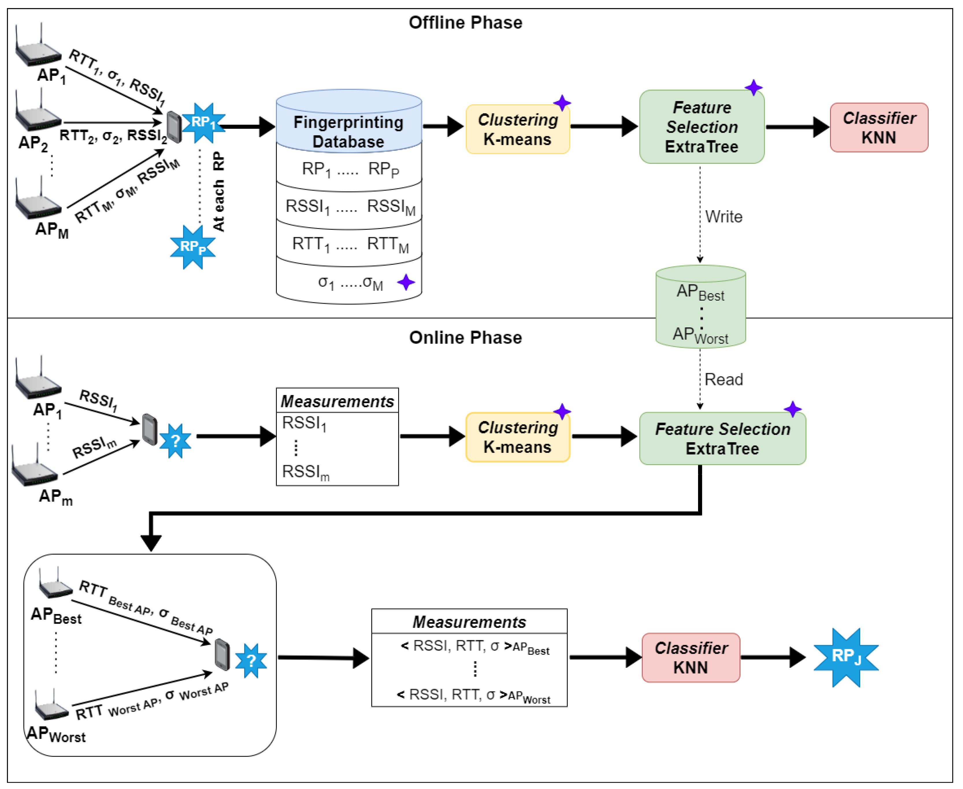
The positioning system proposed in this paper is illustrated in Figure 2. In both offline and online phases, four stages are defined: measurement collection, clustering, feature selection, and classification. This architecture expands upon the one used in our previous research [18] by incorporating the following novelties (highlighted with a purple star in Figure 2): (1) the STD ($\sigma$) of RTT measurements is used as an additional metric; (2) a clustering stage prior to the feature selection is introduced; and (3) in the feature selection stage, different strategies are assessed with respect to the one employed in [18]. Section 3.1 provides a more detailed description of each one of the four stages that comprise the proposed architecture. The specific data models proposed in this paper for each stage are described in Section 3.2. Note that in Figure 2, the measurements are taken twice in the online phase: further details and the reason why it is proposed are given in Section 3.1. Also, note that the “distance obtained through Wi-Fi RTT” is simplified as “RTT” from this point on in this paper.

3.1. General Description

Any FP solution begins with the measurement collection for the construction of the FP database. For that, a grid of P Reference Points (RPs) must be defined in the considered area, where M APs supporting Wi-Fi RTT are deployed. At each RP (i.e., from $R{P}_1$ to $R{P}_P$), the UE pings each available AP and receives the necessary measurements that are then stored in the database. Typically, when constructing the FP database in the offline phase, the measurements at each RP are taken several times, for statistical reasons. The stored measurements may depend on the specific implementation; the ones used in this paper can be found in Figure 2 and are detailed in Section 3.2, so to keep the description here as generic as possible. As commented before, we propose to split the measurement collection in the online phase in two: first, a preliminary scan is performed to gather all the passive measurements (i.e., those that do not need to exchange extra frames with respect to the normal Wi-Fi procedure) from all the Wi-Fi RTT-compatible APs; these measurements are used in the clustering stage to determine the cluster to which they belong. Depending on the geometry or other factors, the UE may be able to gather information from a subset m of the M APs. Moreover, the accuracy of the measurements can vary based on the frequency band in which the APs operate [11,35]. Consequently, m is determined based on the specific conditions and requirements of the location service and can be $m\le M$. Once the feature selection has provided the list of the m APs ordered from the most important to the least, the UE now takes active measurements (i.e., those that inject specific location frames) with the APs in the list. Note that these active measurements may be taken with a subset of the m APs, as is better understood in Section 3.2. Thus, this novel methodology for the measurement collection in the online phase, proposed for the first time in the literature, allows us to foster scalability in the proposed IPS, as it may not be necessary to gather Wi-Fi RTTs with all the APs in sight.

Clustering is an unsupervised ML technique that partitions the data into subsets or ”clusters”; entities within the same cluster exhibit greater similarity to each other than to entities in different clusters [36]. This technique helps identifying patterns or structures within a dataset. It facilitates the creation of sub-scenarios (i.e., clusters) within the overall scenario, thereby augmenting the comprehension of each cluster’s distinctive attributes and enabling more precise analysis and decision-making. In this paper, we propose adding a clustering stage before feature selection with the aim of reducing the number of possible RPs where the UE may be located; in this way, we expect reducing the search space and consequently improving the precision of the classifier. However, it is important to highlight that the clustering stage associates each fingerprint (i.e., the measurements obtained at a given time from each AP by UE located at a given RP) to a given cluster; this allows for a given set of measurements taken at different times from the same RP to be associated to different clusters, thus potentially reducing the benefit mentioned before. Nevertheless, another potential benefit has been identified. When using clustering, feature selection is then applied to the subset of information that belongs to a given cluster. In this way, we expect that the most important AP in a given cluster will be different from the most important AP in another cluster. If this is the case, user devices associated to different clusters would not interfere with each other when performing active measurements for localization purposes, thus enhancing scalability. Instead, in case the same AP is identified as the best one in more than one cluster, a bottleneck may be created in the network, as user devicesin different clusters would all send location traffic to the same AP, thus invalidating the benefits of the clustering stage. The latter can be assessed by observing how the location traffic overhead distributes among all the available APs when a given number of clusters are created and is explored in Section 6.

The feature selection stage entails identifying the most relevant features in the FP database and delivering a list of the selected features, ordered according to the importance score obtained, from the most relevant feature (i.e., ${\mathrm{AP}}_{Best}$) to the least one (i.e., ${\mathrm{AP}}_{Worst}$). The measurements taken with each AP should be understood as features in this context. This process reduces dimensionality, enhances accuracy, prevents overfitting, and increases interpretability [37]. This is achieved by removing irrelevant or redundant features, focusing on meaningful attributes, reducing the risk of learning noise, and making the model easier to understand. For this reason, this stage is designed to organize the features in a way that identifies the most relevant sources (i.e., APs). Once the list is created, it helps not only to reduce the number of features used by the classifier, but also it enables the possibility of reducing the number of APs towards which the UE performs active measurements.

The final stage of the IPS is classification, where an ML algorithm is employed to convert the features into accurate position predictions. This is achieved by comparing a new measurement (the data collected by the UE in its current location) with the previously selected features per cluster in the database and predicting the most probable location (i.e., ${\mathrm{RP}}_J$, where J is a value between 1 and P of the RPs in the grid). To ensure a robust and reliable evaluation, mitigating associated biases, we propose to apply a cross-validation technique in this paper. K-Fold cross-validation [38] is a method that divides the dataset into K slices (or “folds”). The classification model is then trained K times, each time using ($K-1$) slices as the training set and the remaining slice as the validation set. This process is repeated K times so that each slice is used exactly once as a validation set. Specifically, stratified K-fold cross-validation [39] was used, which ensures that each fold has approximately the same proportion of classes as the original dataset.

3.2. Data Models

This section provides further details on the specific models proposed and assessed for our positioning system. Since this study focused on FP based on Wi-Fi RTT, the proposed measurements to collect were RTT, its $\sigma$, and RSSI. Thus, in the offline phase, the three measurements were gathered from each of the M Wi-Fi RTT-compatible APs deployed in the scenario, and at each of the P RPs in the grid. In this way, the FP database was created. The idea in this paper was to use different combinations of these measurements (i.e., using only RTT, using only RSSI, or using RTT and $\sigma$, etc.) and different amounts (i.e., using the measurements from all the APs or only a subset of them) and assess the improvement in the performance of the IPS.

The ordered list of measurements was obtained by applying Extra Tree [40,41] individually to each set of measurements (i.e., RTT, RSSI), as already proposed in our previous study [18]. Specifically, two separate lists were generated: one for the most relevant APs based on the RSSI measurements, and one for the most relevant APs based on the RTT measurements. Three approaches were adopted to generate combinations from the individual RTT and RSSI lists. In the first approach, called “Best RTT and Best RSSI”, the best APs in the RTT list and the best APs in the RSSI list were taken separately. This approach replicated the procedure used in our previous research [18]. The second approach, called “Best RTT and its RSSI”, took the RTT list, selected the APs according to this list, and then used the <RTT, RSSI> measurements of those APs. Similarly, the third approach, called “Best RSSI and its RTT”, selected the APs according to the RSSI list and then used the <RSSI, RTT> measurements of those APs. This latter approach can significantly reduce the time required to create the FP database in the offline phase, since collecting RTTs takes much more time than obtaining RSSIs. In addition, estimating the RTTs also reduces the bandwidth available for the usual location services in the Wi-Fi network, which means that this approach can lead to a better user experience. As explained in Section 2, to the best of our knowledge, there is no comprehensive study on the fusion of $\sigma$ and the average RTT. Therefore, since RTT contains more significant information with respect to its STD alone, we decided to take the RTT as the main active feature for sorting both RTT and $\sigma$.

The benefits of introducing a clustering stage were assessed in this paper. In this study, K-means, one of the most popular clustering algorithms [42,43,44], was used. The dataset was divided into k clusters, where k is a user-specified number. Then, at each iteration, it assigned each sample to the cluster with the closest centroid and recalculated the centroids as the mean of the assigned samples. This process was repeated until the centroids did not change significantly, indicating convergence. A novel method is proposed for the first time in the literature, aimed at reducing the Wi-Fi RTT traffic injected in the network. We determined to which cluster a fingerprint belonged to based on the RSSI measurements only. Thus, in the online phase, first the UE gathered the RSSI with all the RTT compatible APs in sight (i.e., m). Those RSSI were sorted from highest to lowest, and then the clustering stage was implemented taking this sorting as an input. According to the cluster to which the UE was associated, a list of the best APs was given, and thus the UE was able to selectively perform Wi-Fi RTT measurements with a reduced number of APs, thus promoting scalability. In our assessment, however, a unique cluster (i.e., k = 1) was employed in the first place, so that we were able to compare the results with those obtained in our previous study [18], where no clustering was applied; in this way, the contribution of coupling the other measurements (i.e., RTT and RSSI) with $\sigma$ could be understood. When no clustering was employed, all the fingerprints in the dataset belonged to the same cluster. The results of this first assessment are presented in Section 5.

To analyze the performance of the clustering stage, in a second step, we evaluated different densities of clusters, from low density (i.e., 2 clusters), middle density, up to high density (i.e., the maximum number of clusters depending on the number of available APs (M)). As the exact numbers depended on the scenario under evaluation, the exact k values used in this study are specified in Section 6. The clusters were formed with the samples collected at the RPs within the same cluster, allowing for the grouping of RPs within that specific cluster. Since not all the samples in an RP necessarily belonged to the same cluster, we established a threshold as a criterion for including the RP in the cluster. Therefore, any RP that had more than 10% of the samples taken within the group was considered part of the cluster. The performance of the IPS when using clustering is assessed in Section 6.

Finally, in the classification stage, we chose the K-Nearest Neighbors (KNN) classifier, which demonstrated high performance in terms of scalability in previous research [18,45]. For deploying the KNN classifier with cross-validation, five folds were used, as this is a commonly employed value [33,46]. Different combinations of measurements were tested in order to assess the performance of the proposed IPS, including different amounts of RTT, alone or with its $\sigma$, as well as varying amounts of RSSI, according to the importance list obtained in the feature selection stage. For example, the combination “1 RTT–0 RSSI” refers to using the first feature in the RTT list. If another RTT was added, thus taking the first two in the RTT list, the combination became “2 RTTs–0 RSSI”. This process was then repeated with the most important RSSI feature, then with two RSSIs, and so on. Additionally, combinations of RTT with its $\sigma$ alongside RSSI were analyzed. For instance, the combination “1 RTT with its $\sigma$–0 RSSI” used the first RTT in the list with its $\sigma$. Similarly, adding the second most important RTT with its $\sigma$ resulted in the combination “2 RTTs with its $\sigma$–0 RSSI”. Finally, also adding the two most important RSSIs, resulted in the combination “2 RTT with its $\sigma$–2 RSSI”.

4. Evaluation Scenario and Metrics

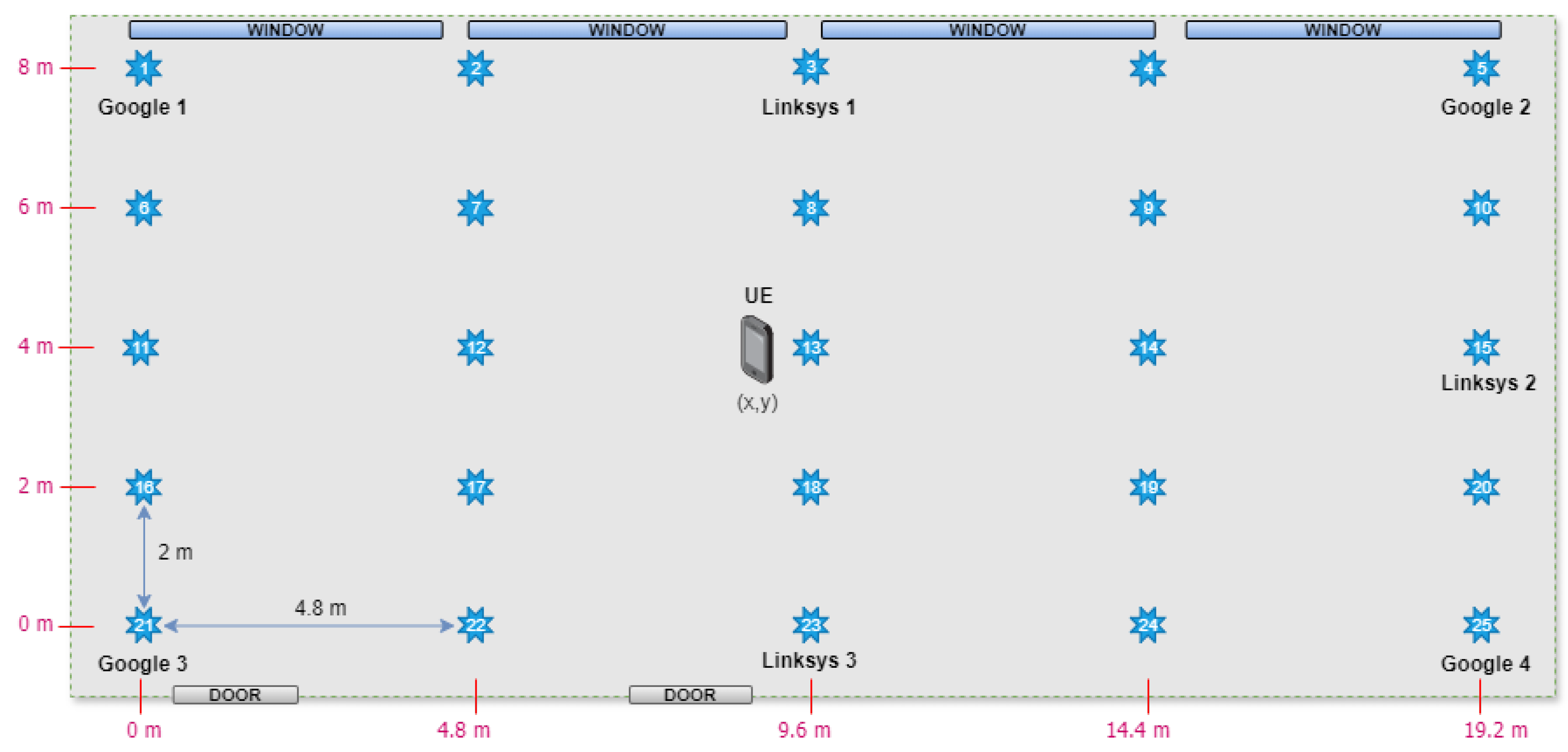
Assessing the system proposed in the previous section necessitates a detailed analysis of its performance within a test environment. To this end, this section outlines the scenario and performance metrics that are essential for evaluating the proposed system. This approach facilitates a comparison between the proposed system and existing solutions, while also allowing for an assessment of its scalability and alignment with the intended objectives. In this context, our research used data from the measurement campaign described in [18]. The samples were collected in one of the auditoria at the Universitat Politècnica de Catalunya. The scenario, as shown in Figure 3, was a rectangular space of 19.2 × 8 m; although direct vision was guaranteed between the different RPs and APs, there were chairs, a big table, and metal frames in this open space, which may interfere with the Line of Sight (LoS). A grid of 5 × 5 RPs (i.e., P = 25) was considered, with each RP at a distance of 4.8 m on the long side and 2 m on the short side; measurements were taken at each RP in the grid. For this purpose, seven Wi-Fi RTT-compatible APs were deployed (i.e., M = 7): four Google APs [47] were placed in the corners, and three Linksys Velop AC6600 [48] in the center of three walls, as shown in Figure 3. Google APs advertise the Wi-Fi RTT feature and only work in the 5 GHz channel 42 (U-NII-1). The Google AP is generally used in the literature due to its well-known compatibility with the IEEE 802.11mc standard [15,18,29,33]. On the other hand, Linksys APs do not advertise the Wi-Fi RTT feature but can respond when pinged; also, they transmit in multiple frequency bands: channel 11 in the 2.4 GHz frequency band and channels 42 (U-NII-1) and 106 (U-NII-2C) in the 5 GHz band. The Google Pixel 3a smartphone, which supports Wi-Fi RTT [20], was used to collect measurements. At each of the 25 RPs, 100 samples were collected for each available AP. Thus, in each frequency band, 2500 samples of RTTs, $\sigma$’s, and RSSIs were collected. Although the Linksys AP can communicate on multiple frequency channels, recent studies have shown that the 5 GHz band indoors (in this case channel 42) offers more accurate and relevant measurements for positioning purposes [11]. Therefore, in this paper, we considered only the measurements obtained in this frequency band from each Wi-Fi RTT compatible AP deployed in the scenario. As a result, our FP database was made up of 21 features: seven RTTs (i.e., one for each AP), seven $\sigma$’s, and seven RSSIs.

In order to assess the performance of the proposed positioning system, we evaluated the RMSE of the estimated positions; the accuracy, recall, precision of the ML model; and the distribution of localization requests between clusters. The RMSE is an indicator of how close the prediction is to the real position, and it is calculated as:

$$\mathrm{RMSE}=\sqrt{{\displaystyle \frac{{\sum }_{i=1}^T{(y_i^{\prime }-y_i)}^2}{T}}},$$

(3)

where T is the number of observations, $y^{\prime }$ is the estimated position, and y is the real position. In other words, it can be thought of as normalizing the distance between the vector of predicted values and the vector of observed values. Also, by squaring the error, the impact of outliers is magnified, thus making the RMSE a solid estimator of the stability of the results. It should be noted that when the number of clusters is greater than one, the RMSE was still calculated for the entire dataset and not for each cluster.

On the other hand, accuracy, precision, and recall report some sort of success rate. Accuracy is determined by the proportion of correct predictions an algorithm makes out of all its predictions. Thus, it represents the chance that the algorithm’s estimated position (the most probable location) exactly matches the actual position of the UE. An accuracy of zero means that no estimated position is actually correct, while an accuracy of one means that every estimated position actually matches the real one. Recall measures the percentage of measurements taken at a given position that are classified in that position. A high recall indicates that the algorithm successfully predicts the user’s actual position whenever the user is at that location. In contrast, a low recall suggests that the algorithm frequently fails to recognize the user’s presence at a given location. Finally, precision calculates the ratio of measurements classified in a given position that are taken in that position. A high precision indicates that when the algorithm classifies the user at a given location, this prediction is usually correct. Conversely, a low precision implies that the algorithm often predicts the user to be at a wrong location. While accuracy provides a general measure of overall correctness, recall focuses on missed detections (false negative classifications) and precision on incorrect identifications (false positive classifications).

On the other hand, in order to analyze the overhead distribution, the percentages of measurements for each cluster and their relationship with the most relevant APs were considered. When the APs that had the greatest influence on FTM traffic within each cluster were identified in the feature selection stage, it was possible to evaluate whether the clustering process was achieving an even distribution of traffic. The percentage of measurements per cluster was calculated as follows:

$$\mathrm{Percentage}={\displaystyle \frac{T{M}_{cluster}}{T{M}_{global}}}\times 100,$$

(4)

where $T{M}_{cluster}$ represents the total number of measurements within a specific cluster, and $T{M}_{global}$ is the total number of measurements across the entire scenario. This formula quantified the proportion of traffic handled by each cluster relative to the overall scenario. By identifying the most relevant APs per cluster, these percentages could be associated with the available APs. If the same AP was identified as the most relevant in several clusters, it could indicate a high concentration of traffic on that AP, potentially leading to an imbalance in the system load. Therefore, in terms of traffic distribution, this analysis not only reflected the effectiveness of clustering but also helped to detect potential bottlenecks that could compromise the scalability of the system.

5. Assessing Performance of Wi-Fi RTT Measurements

This section provides the performance assessment of the positioning system presented in Section 3. Three kind of measurements were considered: RTT, $\sigma$, and RSSI. The way these measurements were considered could impact the performance. Hence, they were prioritized according to their relevance to the scenario through the feature selection stage. The individual lists generated for RTT and RSSI are presented in

Table 1. Individual lists of the 7 most important RTT and RSSI features.

RTT List			RSSI List
AP Name	Score	Position (x, y)	AP Name	Score	Position (x, y)
Linksys 2	0.1780	(19.2, 4)	Google 2	0.1638	(19.2, 8)
Google 4	0.1653	(19.2, 0)	Google 3	0.1541	(0, 0)
Google 2	0.1509	(19.2, 8)	Linksys 2	0.1491	(19.2, 4)
Google 3	0.1422	(0, 0)	Google 4	0.1454	(19.2, 0)
Linksys 1	0.1276	(9.6, 8)	Google 1	0.1384	(0, 8)
Linksys 3	0.1210	(9.6, 0)	Linksys 1	0.1277	(9.6, 8)
Google 1	0.1150	(0, 8)	Linksys 3	0.1214	(9.6, 0)

. Each list shows the AP name, the importance of the contribution of each feature to the predictive model (score), and the position of the AP in the scenario. Section 5.1 focuses on the three proposed approaches in order to generate combinations of these two lists, which are explained in Section 3.2; in order to be able to compare the results with those presented in [18], the $\sigma$ measurements were not taken into account. Section 5.2 takes a step forward by adding the new $\sigma$ measurements to the performance evaluation. It must be noted that clustering was overridden in that section by considering a single cluster (i.e., k = 1). This facilitated the understanding of the impact of the proposed approaches for feature selection and of the newly added measurements $\sigma$ compared to other existing measurements (i.e., RSSI and RTT).

5.1. Coupling RTT and RSSI Measurements

In our previous publication [18], the benefits of using RTT measurements together with the traditional RSSI in FP location systems were assessed. This new paper extends those findings by considering three new approaches for choosing the best sources to feed the ML classification model. In Figure 4, a heatmap of the RMSE obtained with KNN for each approach is depicted; it provides a visual representation of how each model evolves as the number of RTT (on the y-axis) and/or RSSI (on the x-axis) increases. On the color scale, the best results (i.e., smaller RMSE) are plotted in dark red, while dark blue is used for the RMSE values over 2 m, a typical upper bound for indoor location services. It is important to mention that the combination “zero RTT–zero RSSI” had no data and is therefore shown as blank.

Results show that incorporating any feature, either RTT or RSSI, into models with four or more RTTs did not offer significant improvements in terms of RMSE. The values remained within the optimal range (i.e., dark-red area under 0.25 m) and did not exhibit a noticeable reduction in the RMSE as the number of available features increased. Quite the opposite happened when only one RTT was taken (i.e., “one RTT–zero RSSI” in Figure 4), where poor performance was observed (2.71 m RMSE). Under these conditions, adding a feature, either an RTT or RSSI, yielded a significant reduction in the RMSE, with values below 1.50 m (“two RTTs–zero RSSI” and “one RTT–one RSSI” in Figure 4). ML classification models with two or more RTTs produced RMSE values below one meter, regardless of the feature selection approach taken and of the number of other features added.

Focusing on the approach shown on the left, referred to as “Best RTT and Best RSSI”, it can be seen that using two RTTs only (“two RTTs–zero RSSI”) yielded a similar RMSE to the use of all seven available RSSIs (“zero RTT–seven RSSIs”). This indicated that relying on RTT for localization decreased the number of signal sources (i.e., APs) required for localization. Results showed that adding an RSSI was only valuable when less than two RTTs were used. In these scenarios, the more RSSIs sources, the better. However, this pattern was not evident in models using two or more RTTs. In the case of two and three RTTs, adding a single RSSI reduced the RMSE, but incorporating more RSSIs (from two to seven) caused the RMSE figures to randomly oscillate around that reference value (i.e., the one considering a single RSSI). The combinations “two RTTs–one RSSI” and “three RTTs–zero RSSI” showed similar RMSE, which means that the number of features in this case was more important than their nature. Therefore, an RSSI could replace an RTT and hence reduce the overall overhead of the FTM procedure required for positioning. Similarly, using “one RTT–seven RSSIs” yielded the same RMSE, thus reducing the amount of RTTs needed for precise localization, but required a high-density of APs.

The RSSI contribution to RTT, taking into account the APs density, could be better observed when using the two remaining feature selection approaches: “Best RTT and its RSSI” and “Best RSSI and its RTT”. In the former, adding one RSSI to any combination less than four RTTs resulted in a reduction in RMSE. However, going beyond one RSSI did not come with any real improvement in RMSE. Furthermore, we found a higher RMSE for the same RTT–RSSI combinations than in the “Best RTT and Best RSSI”. On the other hand, the results of “Best RSSI and its RTT” showed better performance than the other two approaches, especially when the number of sources was limited (e.g., less than four). For instance, the combination of “three RTTs–zero RSSI” yielded an RMSE of only 0.16 m; notice that adding one or more RSSI features on top of that did not improve the performance. Except for the case when one RTT was used, the best results were obtained without coupling RTTs with RSSIs (i.e., the column with RSSI = 0). This feature selection approach, which used the RSSIs to choose which RTTs to take for the classification ML model, eliminated the need to collect all the available RTTs to identify the most relevant ones. Thus, it significantly reduced the time needed in the offline phase to build the FP database, and at the same time, it noticeably lessened the overhead associated with the RTT data collection.

5.2. Integrating the Standard Deviation

This section addresses the impact of using the STD of the RTT estimation (i.e., $\sigma$) as a new feature feeding our classification ML model; to the best of the author’s knowledge, it represents a novel approach for RTT FP location systems. Figure 5 mimics what was carried out in Figure 4 and thus presents the RMSE of the user’s position according to the feature selection approach applied, but considering this time the new feature $\sigma$.

To analyze the contribution of $\sigma$, we first compared the RMSE when no RSSI was considered. The goal was to assess the enhancement in the RMSE when adding $\sigma$ to pure RTT-based models. This was carried out by comparing the results of the zero-RSSI column in Figure 4, where $\sigma$ was not considered, with those in Figure 5. Results showed that adding $\sigma$ to the classification model clearly reduced the RMSE, especially in those conditions where the number of sources was scarce (i.e., below four RTTs). Except for the combination of “one RTT with its $\sigma$–zero RSSI”, all the other combinations of the RTT with its $\sigma$ were below 0.50 m. Again, as also shown in Figure 4, the more RTTs, the better the RMSE. The real degree of the impact of $\sigma$ in the RMSE depended on two aspects: the number of sources considered and the feature selection approach applied. When only one RTT was taken, the reduction in the RMSE was approximately 36% regardless of the feature selection approach. However, classification models built with two or more RTTs were much more sensitive to how features were selected. Thus, selecting features according to the RSSI (i.e., a third of our approaches, represented on the right of the figures) reduced the effectiveness of adding the $\sigma$ (a reduction in RMSE by approximately 10%). Nevertheless, using $\sigma$ seemed to have a positive impact on the RMSE, regardless of the feature selection approach. In fact, RMSE values presented in Figure 4 were quite similar (differences around 0.07 m), whatever the approach taken to select the features.

When we incorporated RSSI measurements into the “Best RTT with its $\sigma$ and Best RSSI” approach, similar patterns emerged as in the “Best RTT and Best RSSI”. In the case of a single RTT with its $\sigma$, adding RSSI resulted in a decrease in RMSE, although the effect was more gradual. No significant improvements were seen, however, when adding RSSI to two and three RTTs, regardless of the way the feature selection approach was chosen. This behavior suggested that the algorithm could have been suffering from overfitting. In the case of a single RTT, adding one RSSI (“one RTT–one RSSI” in Figure 4) provided more information than adding $\sigma$ (“one RTT with its $\sigma$–zero RSSI” in Figure 5), reaching an RMSE of 1.17 m and 1.73 m, respectively. However, adding both RSSI and $\sigma$ (“one RTT with its $\sigma$–one RSSI”) produced better results (i.e., 1.01 m) than adding only one RSSI. These results revealed that $\sigma$ provided more information when a low amount of information was available, i.e., with a single RTT. However, as the number of RTTs increased, and consequently, the amount of information increased, the contribution of $\sigma$ gradually diminished.

Overall, we identified “Best RSSI and its RTT with its $\sigma$” as the best-performing approach, because it obtained a low RMSE even when few information was available; moreover, it had the added value of reducing the overhead, since it selected the RTTs based on the RSSIs, as discussed in Section 5.1. Among the combinations highlighted for their tradeoff between precision and scalability there were the following: “one RTT with its $\sigma$–1 RSSI”, “2 RTT with its $\sigma$–zero RSSI”, and “three RTTs with its $\sigma$–zero RSSI”. The first combination achieved a precision of 1.01 m RMSE with a single AP, surpassing recent proposals that reached, e.g., an RMSE of 1.17 m [31]. Using the combination “2 RTT with its $\sigma$–zero RSSI”, an RMSE of 0.38 m was achieved, which was comparable to the 0.33 m achieved in [33] using DNN and Random Forest (RF) with three APs. This suggested that with one fewer AP and a less complex algorithm, similar results could be achieved with our approach; moreover, when we used three APs, the RMSE decreased to 0.13 m, more than half the results obtained in [33] with the same number of sources. Furthermore, the three highlighted combinations showed better performance than the use of RTT with RSSI in multilateration, as proposed in [26], where an error of 1.03 m was obtained. It must be stressed here that most importantly, these three highlighted combinations reduced the overhead of Wi-Fi RTT and showed promising performance in the tradeoff between scalability and precision.

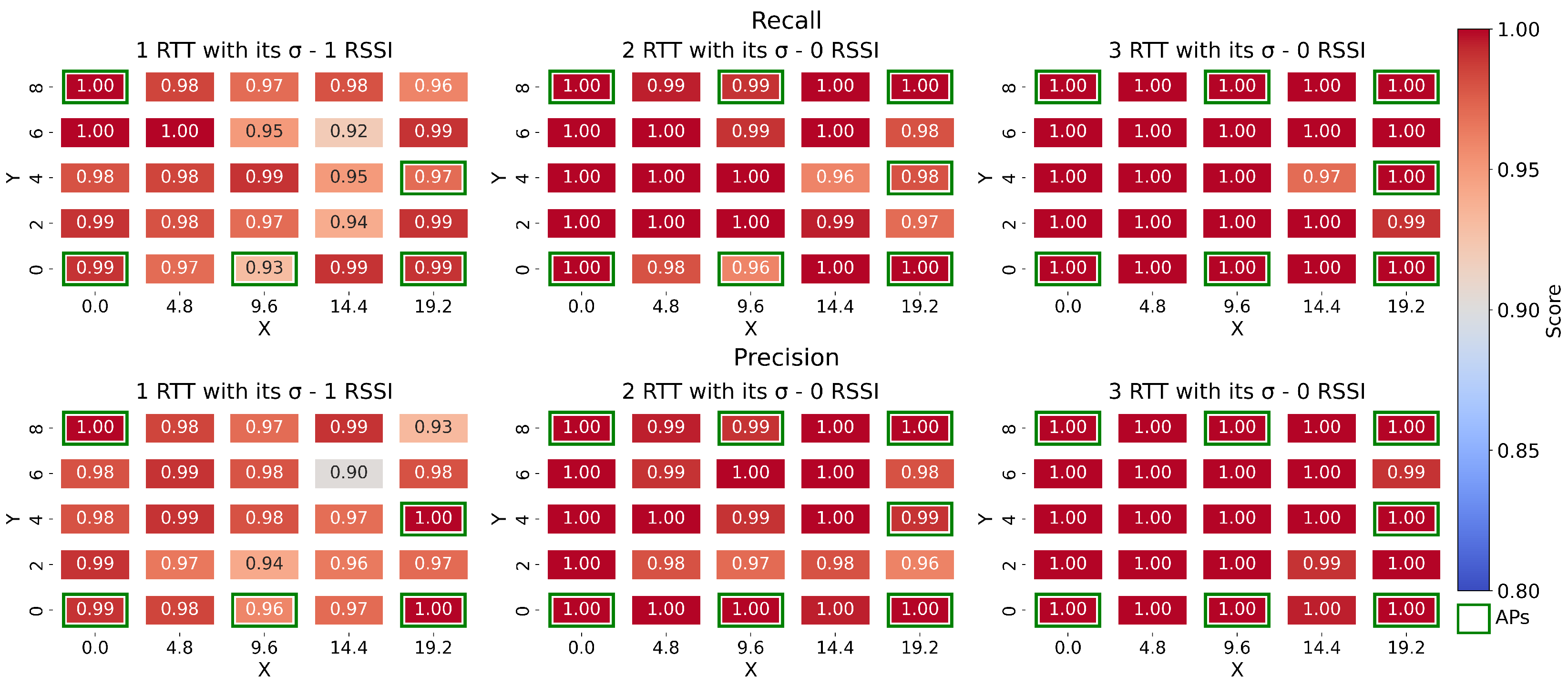
On the other hand, the classifier showed high accuracy: 94.92% for “one RTT with its $\sigma$–one RSSI”, 98.44% for “2 RTT with its $\sigma$–zero RSSI”, and 99.56% for “three RTTs with its $\sigma$–zero RSSI”. In order to complete the analysis on the performance of the classifier, the recall and precision are shown in Figure 6. The X-axis represents the length (from 0 to 19.2 m), while the Y-axis the width (from 0 to 8 m) of the scenario. The color scale is set so that the minimum (in dark blue) is 0.80, and the maximum (in dark red) is 1.00. Also, the locations of the most relevant APs, according to the feature selection, are marked with a green outline; this visual indication allows for the quick identification of the infrastructure actually needed for location purposes. The recall is shown at the top, while the precision is shown at the bottom in Figure 6. In the combination “one RTT with its $\sigma$–one RSSI” (on the left), it is evident that the classifier is more likely to deliver a wrong estimation for those RPs that are in the upper part of the diagonal formed from (0.0, 8) to (19.2, 0) (i.e., top right side of the scenario, and close to the most relevant AP). For instance, for RP (14.4, 4), the recall had a score of 0.86, and 0.87 for the precision. A recall of 0.86 means that 86% of the location measurements taken from that RP were correctly classified at RP (14.4, 4), while 14% were classified in another RP. On the other hand, a precision score of 0.87 means that 87% of the user devices that were classified in that RP were actually located at that RP, while 13% were classified at that RP but were located elsewhere.

Both precision and recall increased when we added new features. In the combination “two RTTs with their $\sigma$–zero RSSI” (plots in the middle) the recall was below 0.90 for one RP only (i.e., (14.4, 6)); however, the precision in that RP was 0.94. RP (14.4, 8) showed the lowest precision (0.90) and a recall of 0.94. These results obtained in such close RPs suggested that the classifier tended to confuse the values of RP (14.4, 6) with those of RP (14.4, 8). For the combination of “three RTTs with their $\sigma$–zero RSSI” (on the right) all the scores of both metrics were above 0.96, showing that the misclassification was clearly reduced in all the area.

However, the overall RMSE presented was not uniform across all RPs in our scenario, despite being an LoS environment. This is evidenced in Figure 7, which shows the RMSE performance at each RP in our scenario for the three highlighted combinations (i.e., tradeoff between precision and scalability). The scale used was the same as in Figure 4, which facilitated the analysis of the results. To calculate the RMSE, only the 100 samples taken at each RP along with their respective predictions were considered. Figure 7 revealed a critical zone at X equals to 14.4, where it was observed that the KNN algorithm was prone to fail. For the combination “one RTT with its $\sigma$–one RSSI”, the RMSE was below one meter in 14 of the 25 RPs; on the other hand, in 4 RPs it exceeded 1.50 m, limiting the applicability of our system for stringent localization services that need to guarantee an RMSE below one meter. Note that the most relevant AP in this combination was the one in the upper right corner, at (19.2, 8). The combination “2 RTT with its $\sigma$–zero RSSI” coped with this limitation, reducing the RMSE at all RPs and leaving only one RP (14.4, 8) above one meter (1.07 m). Additionally, 21 out of 25 RPs presented an RMSE below 0.50 m, of which 15 had an RMSE of 0 cm. Although the critical zone (i.e., X = 14.4) was reduced, it remained the area with the highest RMSE. On the other hand, the combination “three RTTs with its $\sigma$–zero RSSI” achieved an RMSE below 0.50 m at all RPs, with 80% of the RPs (20 RPs) having an RMSE of 0 cm. The latter results were promising but presented the limitation that the three APs marked in green were used for positioning, whatever the UE’s position in the room. This can imply a burden of location traffic in areas of high service demand: all the users would exchange FTM frames with these three APs instead of distributing them among different APs. Thus, using a fixed selection of APs may impact the bandwidth available for location services in certain APs. Therefore, in high-density scenarios like the one presented in this paper, where seven APs were available in an area of almost 154 m², not utilizing all the available sources of location information could hinder the system’s ability to manage high demand for location services, potentially affecting the quality of service. To make better use of these resources, the implementation of a clustering stage in Wi-Fi RTT FP is proposed and discussed in Section 6.

6. Clustering for a Precise and Scalable Positioning System

After assessing the impact of integrating $\sigma$ and the use of different approaches for selecting the most valuable information sources (i.e., feature selection stage), this section focuses on the scalability of the positioning model. This was achieved by means of the clustering stage (see Figure 2). Clustering divided the positioning area into smaller sections, with only a subset of the available RPs. The aim of this approach was twofold. First, it allowed the feature selection stage to be focused only on a reduced subset of RPs. Ideally, these subsets would be different from cluster to cluster, thus making the classification task easier and more effective. Second, the overhead of localization traffic (i.e., RTT requests) was expected to be distributed more evenly, which should boost the scalability of the localization system. This section analyzes the different clustering sizes k and their contributions to the positioning accuracy. In Section 6.1, the impact on accuracy when applying this new stage to the FP is evaluated, with particular emphasis on cases where we used one RTT per cluster. The distribution of FTM traffic among the available APs under these challenging conditions is examined in Section 6.2. Finally, the performance across the RPs within our scenario is discussed in Section 6.3.

6.1. Impact of Applying Clustering

Similarly to Figure 5 presented in Section 5, Figure 8 shows the heatmap of the RMSE for different number of clusters. In this case, only the model considering the “Best RSSI and its RTT with its $\sigma$” approach for feature selection was taken into account, as it provided the best results in Section 5. This choice reduced the ramification of the study and allowed us to focus on the impact of clustering. Five clustering sizes (i.e., k) were considered: one, two, four, five, and seven. These sizes allowed us to study the impact of clustering when the cluster area was gradually reduced: the greater the number of clusters, the smaller the cluster became. k equal to one, which means no clustering, was deeply analyzed in Section 5 and it is included as reference for comparison. We then started by increasing k to two, so that the area was divided into two large clusters. This allowed us to observe initial changes in localization traffic distribution and potential improvements in accuracy, thanks to a reduced area per cluster. The intermediate values of $k=4$ and $k=5$ represented moderate cluster densities. With smaller clusters, we expected the positioning precision to increase and the location traffic load to be better balanced among APs. Finally, $k=7$ corresponded to the total number of Wi-Fi RTT-compatible APs that were available in the scenario. This latter situation enabled location traffic to ideally be uniformly distributed among the APs. Increasing k beyond this limit would not have provided any clear benefit from the point of view of traffic distribution. For this reason, we considered seven as the maximum number of clusters for the scenario under consideration.

The analysis was limited to four RTTs per cluster, based on the findings of the previous section, to allow a better visualization of the results. This limitation facilitated the interpretation and comparison of the effects of different k values on the AP distribution and the precision of the localization system. The results in Figure 8 show that clustering did not significantly improve the RMSE of the position estimates when three or more RTT sources with their $\sigma$ were considered. Under these conditions, the slight fluctuations in the RMSE were due to noise associated with the estimates used for validation. The same was true when six or more RSSI sources were considered. In scenarios where the sources of information were limited (i.e., one or two), clustering led to a reduction in the RMSE of the estimated positions. In terms of number of clusters, results became better as long as k increased; however, when the maximum value of seven was reached, the RMSE seemed not to improve any longer.

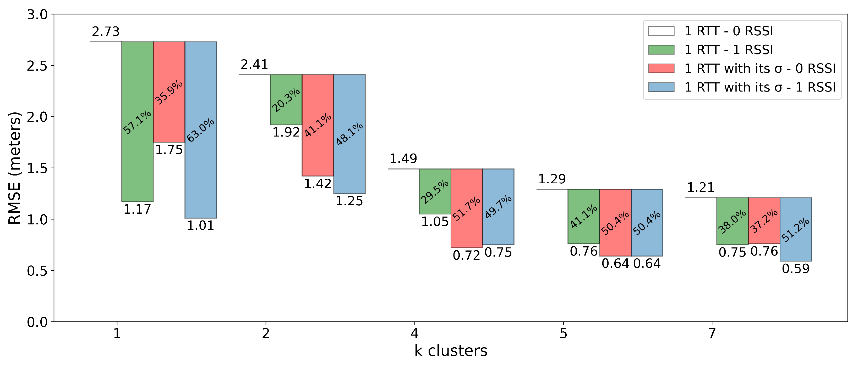
For a better comparison, Figure 9 shows the contribution of the RSSI and $\sigma$ to the RTT, according to the clustering size. Only one RTT was considered there, as it was the most challenging scenario and therefore, where the impact of either $\sigma$ and clustering on the RMSE was expected to stand out the most. The horizontal axis (i.e., X) sets the clustering size (i.e., k), while the vertical axis (i.e., Y) shows the RMSE in meters. The bars represent different configurations: in green, the addition of one RSSI to the RTT; in red, the inclusion of the $\sigma$ of the RTT under consideration; and in blue, the incorporation of both features. Within each bar, the percentage of RMSE reduction is shown compared to the reference combination, where only one RTT was considered (“one RTT–zero RSSI”). When $k=1$ in Figure 9, the RSSI (in green) contributed more information than $\sigma$ (in red), with a reduction of 57.1% and 35.9%, respectively. However, when using both features (in blue), the reduction was even higher (63%). This suggested that when no clustering ($k=1$) was employed, the combination of RSSI and $\sigma$ was more effective. The opposite behavior was observed when considering clustering (i.e., k > 1). In these cases, the RSSI tended to contribute less information compared to $\sigma$, except when $k=7$, where the contribution was almost even. Moreover, the combination of both features along with RTT proved to perform as good as, or even better than, adding $\sigma$ only. In these cases, the reduction was always around 50%, whatever the number of clusters. Although increasing the value of k in the combination “one RTT–zero RSSI” improved the RMSE, results below one meter were not achieved. To achieve this, k had to be greater than or equal to four, and RSSI, $\sigma$, or both had to be added.

Similarly, Figure 10 shows the accuracy for the same combinations as in Figure 9. On the one hand, when clustering was not included (i.e., k = 1), adding at least one new feature already brought a considerable improvement to the accuracy; when one RSSI and one $\sigma$ were added (in blue), the accuracy almost reached 95%. On the other hand, increasing the number of clusters improved the accuracy, except when k = 7; in the latter scenario, the accuracy decreased in all the cases with respect to k = 5, except when one RSSI and one $\sigma$ were added.

In summary, while the use of the RSSI provided more information when $k=1$, $\sigma$ showed a consistent increasing contribution as the number of clusters increased, especially with $k=4$ and $k=5$. The combination of $\sigma$ and RSSI tended to be more effective in reducing the error, although this effectiveness varied depending on the value of k. Additionally, this RMSE analysis revealed that the application of clustering did not introduce additional errors to the system; on the contrary, it improved the performance when compared to the use of a single RTT per cluster. These findings allowed us to proceed further, focusing on the goal of distributing FTM traffic among the available APs, so that scalability was boosted.

6.2. Distribution of the Overhead Among the Available APs

In the previous section, the RMSE performance for different k sizes was analyzed, with a particular focus on the case of using a single AP. In this section, the evaluation continued using a single AP per cluster; this allowed us to assess the benefits of clustering in terms of the distribution of location traffic (i.e., RTT requests) overhead.

Table 2. Distribution of the location traffic overhead among the most relevant APs for each cluster size. The highest percentage for each cluster size is highlighted in bold.

k	Google 3	Google 4	Linksys 2	Linksys 3	Google 1	Google 2	Linksys 1
2	57.80%	42.20%	-	-	-	-	-	100%
4	25.88%	15.96%	24.12%	34.04%	-	-	-	100%
5	16.16%	15.96%	24.12%	27.92%	15.84%	-	-	100%
7	15.96%	25.96%	12.08%	24.00%	-	22.00%	-	100%

presents the distribution of the location traffic overhead among the most relevant APs for each cluster size, i.e., the relative number of measurements, out of the total of 2500 (100%), where the most relevant AP was the one under consideration. One would expect that for each cluster size k, the percentages of measurements would be evenly distributed across clusters. However, these percentages fluctuated around $\pm 10\%$ of the expected values. Although a single AP (highlighted in bold in Table 2) tended to dominate for each k, this AP was not always the same and depended on the specific value of k. It is important to note that in the case of $k=7$, where one might have expected a single AP per cluster, only five APs were identified as the most relevant, with a distribution similar to that seen with $k=5$. This result discouraged cluster configurations with k beyond five for the scenario under evaluation. On the other hand, the fluctuations in the distribution of percentages across APs revealed that although each AP used in $k=4$ presented lower percentages than those used in $k=2$, the maximum difference in percentages between clusters was greater in $k=4$: it was 18.08% between Linksys 3 and Google 4 when k = 4, and 15.60% when $k=2$. With $k=5$, the percentage difference between the AP with the most of the location traffic and the one with the least was reduced to 12.08% (i.e., Linksys 3 and Google 1).

Introducing clustering clearly changed the dominance of some AP. While Google 2 was the most relevant AP in the RSSI list when no clustering was applied (see Table 1), it did not always remain so when clustering was introduced, being the most relevant only for $k=7$ with 22%. Notably, Linksys 1 turned out to be irrelevant in any cluster, despite its similar score to Linksys 3 in the feature selection lists in Table 1. In contrast, Google 3 and Google 4 were present at all values of k chosen, although as k increased, the percentage of location traffic for Google 3 tended to decrease.

At this point, it was interesting to observe how many user devices could obtain FTM measurements from a given AP simultaneously. As already commented in the introduction, an upper bound exists, and it is set to 30 user devices when the location rate is one per second [17]. Our rationale for applying clustering was that it helped the IPS to scale better when the number of simultaneous users increases. Ideally, then, with two clusters, we would be able to double the upper bound, because ideally, we would be able to orchestrate the FTM requests so that half of the user devices interrogate one AP and the other half another AP. However, from Table 2, we observe that the location traffic did not equally distribute among clusters.

Table 3. Comparison between the number of user devices simultaneously located by the proposed Wi-Fi RTT system and the maximum values for different cluster sizes (k). The upper bound was set to 30 user devices able to simultaneously send one FTM per second with one AP (i.e., $k=1$) [17].

k	Simultaneous User Devices	Maximum	Difference (%)
2	52	60	13.33%
4	88	120	26.66%
5	107	150	28.66%
7	116	210	44.76%

shows to what extent increasing the clustering size (k) actually boosted the scalability of the system; the number of user devices that were actually able to simultaneously send FTMs was calculated by dividing the upper bound by the maximum location overhead (i.e., the values marked in bold in Table 2) for each value of k. Again, while increasing the cluster size k, the number of simultaneous user devices increased too; however, the difference between the observed and the maximum values also increased. We observed that with k = 7, there was a considerably smaller increase in the number of simultaneous user devices compared with k = 5. Based on the distribution of traffic and the overall RMSE values obtained (see Figure 9), we can conclude that the number of clusters with more scalable performance was $k=5$.

6.3. Spatial Distribution of the RMSE

In this section, the RMSE, recall and precision per RP was assessed when applying the K-Means clustering algorithm with k = 5. Compared to Figure 6 and Figure 7, after applying clustering, a significant improvement in the performance was observed, as shown in Figure 11 and Figure 12, for most of the RPs. The recall and precision results for the combination “one RTT with $\sigma$–one RSSI” (left plots in Figure 11) exceeded 0.90 for all RPs; only three RPs had a score below 0.95 in both recall and precision. Among them, RP (14.4, 6) showed the worst performance in both metrics. For the combination “two RTTs with $\sigma$–zero RSSI” (plots in the middle), all RPs presented a score above 0.95. These results were similar to those when using “three RTTs with $\sigma$–zero RSSI” when clustering was not applied (see plots on the right in Figure 6). Even better scores were observed for the combination “three RTTs with $\sigma$–zero RSSI” (plots on the right), with values always close or equal to 1.00. These high scores indicated that the system made very few misclassifications. However, when errors did occur, they became more evident in the RMSE due to the grid spacing, which was 4.8 m along the X-axis and 2 m along the Y-axis.

Thus, analyzing the RMSE was necessary in order to better understand the magnitude of the error when the algorithm was not able to provide an accurate estimate. Figure 12 shows the RMSE for our scenario. In the combination “one RTT with $\sigma$–one RSSI”, it was possible to achieve location accuracy with an error margin under 1.50 m across all RPs, as the maximum RMSE observed was 1.43 m at coordinates (14.4, 6). Additionally, 22 RPs achieved an error of less than one meter. The advantage of implementing clustering before feature selection paved the way for identifying five different APs (marked in green in Figure 12). Each one was the most relevant in its cluster. This ensured that users in different clusters would not interfere among each other when measuring the RTT. In contrast, for the combinations “two RTTs with $\sigma$–zero RSSI” and “three RTTs with $\sigma$–zero RSSI”, a different subset of APs in each cluster was used, thus all available APs could intervene in the localization process. Additionally, the location traffic was better distributed; this was an improvement with respect to the case when no clustering was implemented (Figure 7). For the combination “two RTTs with $\sigma$–zero RSSI”, the RMSE was always below one meter. Additionally, only three RPs exceeded 0.50 m, with the worst case at (19.2, 2) with 0.60 m. Notice that the critical zone identified in Figure 7 was eliminated with clustering, thus achieving a more uniform precision throughout all scenarios. Moreover, when we compared the RMSE at each RP between the first two combinations, the RMSE always decreased, except at (19.2, 6) and (19.2, 2), where it increased by 0.20 m. In case we needed to guarantee an error below 0.50 m for all RPs, the combination “three RTTs with $\sigma$–zero RSSI” had to be employed; except two RPs, the RMSE dropped to 0 cm in the whole area. The three combinations analyzed provided a reduction in errors, along with a more distributed use of the available APs. These improvements compared favorably to the results of these same combinations in Section 5.1, where no clustering was applied (see Figure 7). Therefore, we can conclude that the integration of $\sigma$ and the implementation of a clustering stage give positioning systems based on Wi-Fi RTT FP an improvement in their scalability and precision.

7. Conclusions and Future Work

Although the range estimation procedure introduced in IEEE 802.11mc was a marked improvement in terms of accuracy and response time, its P2P nature can drastically affect the throughput available for data services. This is especially relevant when using the traditional multilateration approach, where multiple measurements are often required to cope with all kinds of errors (e.g., multipath, signal blocking, geometric dilution of accuracy, etc.). Using RTT as input for Wi-Fi FP location systems seems to provide as good or even better results than traditional multilateral solutions. It is more insensitive to NLoS conditions and keeps the location traffic overhead under control. Furthermore, it can be more capable under challenging reception conditions, providing accurate enough positions with limited APs in sight. However, while the reduction in the number of RTT measurements improves scalability, it often comes with a reduction in the precision of the computed positions. Therefore, coupling RTTs with other passive measurements is generally a good approach in order to improve positioning accuracy. This study followed this approach and analyzed the performance achieved by combining RTT and RSSI measurements, together with the STD of the RTT (i.e., $\sigma$), under a KNN-based FP classification model. The addition of $\sigma$ showed significant improvements in terms of precision, especially under limited coverage. Thus, RMSE values of 1.01 m were achieved with a single AP, surpassing previous proposals. These results are clearly beneficial in real-world environments, such as hospitals or airports, where the available APs are the minimum necessary for communications; however, location services should be provided to a large number of users. The use of $\sigma$ in RTT measurements enhances system performance by ensuring precise location estimates even with limited infrastructure, thereby minimizing the need for additional APs and reducing location-specific traffic.

The choice of the best features for the classification model from passive measurements is also a contribution of this paper. We showed that the RSSI could be effectively used to weight the relevance of RTT APs, which was a way to simplify the deployment and maintenance of the localization system. This was further enhanced by incorporating a clustering stage based on RSSI in the FP process. The implementation of this clustering stage, aimed at distributing traffic among the available APs, showed promising results. The K-Means algorithm, with different values of k, was used, leading to $k=5$ as the most relevant cluster size for scalability’s sake, considering one single AP per cluster. With this configuration, RMSE values of 0.64 m were obtained, and an overhead distribution close to 20% ($\pm 10\%$) was achieved. Furthermore, a localization service with a precision of less than 0.60 m at each RP was achieved using two RTTs with their $\sigma$ per cluster. This mitigated critical zones in the scenario. Using three RTTs with their $\sigma$, the RMSE did not exceed 0.50 m at any RP. It achieved a global RMSE value of 0.11 m, significantly improving existing multilateration solutions with the same amount of overhead.

Despite the promising results, this study has several limitations. One is using the measurements gathered with a single device (UE). As measurement accuracy and therefore $\sigma$ behavior can depend on the specific device, extending this study with a greater set of devices is planned for future work. Additionally, the inclusion of a clustering stage increases the complexity of the algorithm, which may negatively affect its response speed and training time. In the interest of reducing the complexity of the model, one step could be to explore the possibility of selecting the cluster based on the RSSI of the most relevant AP, thus eliminating the need for more complex clustering algorithms and feature selection. This study also marks the first steps in the integration of $\sigma$ but it does not delve into a comprehensive theoretical analysis of the relationship between RTT and its $\sigma$. Understanding this relationship could allow us to find out other ways of coupling these two features, reaching a more powerful and/or simple magnitude that leads to better-performing positioning models. In addition, consideration should be given to incorporating passive features from different technologies, such as UWB or BLE, which would result in potentially more scalable and accurate positioning systems. Future research should address these limitations, including a detailed analysis of the models in environments with NLoS conditions.

References

1. Qi, L.; Liu, Y.; Yu, Y.; Chen, L.; Chen, R. Current Status and Future Trends of Meter-Level Indoor Positioning Technology: A Review. Remote Sens. 2024, 16, 398. [Google Scholar] [CrossRef]
2. Retscher, G. Fundamental Concepts and Evolution of Wi-Fi User Localization: An Overview Based on Different Case Studies. Sensors 2020, 20, 5121. [Google Scholar] [CrossRef]
3. Yin, H.; Xu, X.; Lu, S.; Chen, X.; Xiong, R.; Shen, S. A Survey on Global LiDAR Localization: Challenges, Advances and Open Problems. Int. J. Comput. Vis. 2024, 132, 3139–3171. [Google Scholar] [CrossRef]
4. Khan, D.; Cheng, Z.; Uchiyama, H.; Ali, S.; Asshad, M.; Kiyokawa, K. Recent advances in vision-based indoor navigation: A systematic literature review. Comput. Graph. 2022, 104, 24–45. [Google Scholar] [CrossRef]
5. Hanssens, B.; Plets, D.; Tanghe, E.; Oestges, C.; Gaillot, D.P.; Liénard, M.; Li, T.; Steendam, H.; Martens, L.; Joseph, W. An Indoor Variance-Based Localization Technique Utilizing the UWB Estimation of Geometrical Propagation parameters. IEEE Trans. Antennas Propag. 2018, 66, 2522–2533. [Google Scholar] [CrossRef]
6. Ma, W.; Fang, X.; Liang, L.; Du, J. Research on indoor positioning system algorithm based on UWB technology. Meas. Sens. 2024, 33, 101121. [Google Scholar] [CrossRef]
7. Zafari, F.; Gkelias, A.; Leung, K.K. A Survey of Indoor Localization Systems and Technologies. IEEE Commun. Surv. Tutor. 2019, 21, 2568–2599. [Google Scholar] [CrossRef]
8. Suryavanshi, N.B.; Viswavardhan Reddy, K.; Chandrika, V.R. Direction Finding Capability in Bluetooth 5.1 standard. In Proceedings of the Ubiquitous Communications and Network Computing: Second EAI International Conference, Bangalore, India, 8–10 February 2019; Proceedings 2. Springer: Berlin/Heidelberg, Germany, 2019; pp. 53–65. [Google Scholar]
9. Jin, Z.; Li, Y.; Yang, Z.; Zhang, Y.; Cheng, Z. Real-Time Indoor Positioning Based on BLE Beacons and Pedestrian Dead Reckoning for Smartphones. Appl. Sci. 2023, 13, 4415. [Google Scholar] [CrossRef]
10. Yaro, A.S.; Maly, F.; Prazak, P. A Survey of the Performance-Limiting Factors of a 2-Dimensional RSS Fingerprinting-Based Indoor Wireless Localization System. Sensors 2023, 23, 2545. [Google Scholar] [CrossRef]
11. Martin-Escalona, I.; Zola, E. Improving Fingerprint-Based Positioning by Using IEEE 802.11 mc FTM/RTT Observables. Sensors 2022, 23, 267. [Google Scholar] [CrossRef]
12. IEEE Std 802.11-2016 (Revision of IEEE Std 802.11-2012); IEEE Standard for Information Technology—Telecommunications and Information Exchange between Systems Local and Metropolitan Area Networks—Specific Requirements—Part 11: Wireless LAN Medium Access Control (MAC) and Physical Layer (PHY) Specifications. IEEE: New York, NY, USA, 2016; pp. 1–3534. [CrossRef]
13. Martin-Escalona, I.; Zola, E. Ranging Estimation Error in WiFi Devices Running IEEE 802.11mc. In Proceedings of the GLOBECOM 2020-2020 IEEE Global Communications Conference, Taipei, Taiwan, 7–11 December 2020; pp. 1–7. [Google Scholar]
14. Horn, B.K. Doubling the Accuracy of Indoor Positioning: Frequency Diversity. Sensors 2020, 20, 1489. [Google Scholar] [CrossRef]
15. Hashem, O.; Harras, K.A.; Youssef, M. Accurate Indoor Positioning Using IEEE 802.11mc Round Trip Time. Pervasive Mob. Comput. 2021, 75, 101416. [Google Scholar] [CrossRef]
16. Feng, X.; Nguyen, K.A.; Luo, Z. Wifi Access Points Line-of-Sight Detection for Indoor Positioning Using the Signal Round Trip Time. Remote Sens. 2022, 14, 6052. [Google Scholar] [CrossRef]
17. Banin, L.; Bar-Shalom, O.; Dvorecki, N.; Amizur, Y. Scalable Wi-Fi Client Self-Positioning Using Cooperative FTM-Sensors. IEEE Trans. Instrum. Meas. 2019, 68, 3686–3698. [Google Scholar] [CrossRef]
18. Gonzalez Díaz, N.; Zola, E.; Martin-Escalona, I. Assessing the Impact of Coupling RTT and RSSI Measurements in Fingerprinting Wi-Fi Indoor Positioning. In Proceedings of the Int’l ACM Conference on Modeling Analysis and Simulation of Wireless and Mobile Systems, Montreal, QC, Canada, 29 October–2 November 2023; pp. 19–26. [Google Scholar]
19. Corrêa Oliveira, D.; Zola, E.; Martin-Escalona, I. Impact of the Burst Size on the FTM Procedure in Android Phones. In Proceedings of the Int’l ACM Conference on Modeling Analysis and Simulation of Wireless and Mobile Systems, Montreal, QC, Canada, 29 October–2 November 2023; pp. 205–208. [Google Scholar]
20. Wi-Fi Location: Ranging with RTT. Available online: https://developer.android.com/develop/connectivity/wifi/wifi-rtt#supported-phones (accessed on 1 July 2024).
21. Horn, B.K. Indoor Localization Using Uncooperative Wi-Fi Access Points. Sensors 2022, 22, 3091. [Google Scholar] [CrossRef]
22. Truong, H.; Justin, L.X.K.; Anish, G.A.; Balan, R.K. Applicability and Challenges of Indoor Localization Using One-Sided Round Trip Time Measurements. In Proceedings of the Workshop on Body-Centric Computing Systems, Tokyo, Japan, 3–7 June 2024; pp. 1–6. [Google Scholar]
23. Dong, Y.; Shi, D.; Arslan, T.; Yang, Y. Error Investigation on Wi-Fi RTT in Commercial Consumer Devices. Algorithms 2022, 15, 464. [Google Scholar] [CrossRef]
24. Google LLC. Wi-Fi RTT (IEEE 802.11mc). Available online: https://source.android.com/docs/core/connect/wifi-rtt (accessed on 1 July 2024).
25. Guo, G.; Chen, R.; Ye, F.; Peng, X.; Liu, Z.; Pan, Y. Indoor Smartphone Localization: A Hybrid WiFi RTT-RSS Ranging Approach. IEEE Access 2019, 7, 176767–176781. [Google Scholar] [CrossRef]
26. Dong, J.; Rana, L.; Cui, S.; Li, J.; Hwang, J.; Park, J. Investigation on Indoor Positioning by Improved RTT-RSS Fusion Ranging Method. In Proceedings of the 2023 IEEE 6th International Conference on Electronics and Communication Engineering (ICECE), IEEE, Xi’an, China, 15–17 December 2023; pp. 49–53. [Google Scholar]
27. Ma, C.; Wu, B.; Poslad, S.; Selviah, D.R. Wi-Fi RTT Ranging Performance Characterization and Positioning System Design. IEEE Trans. Mob. Comput. 2022, 21, 740–756. [Google Scholar] [CrossRef]
28. Choi, J.; Choi, Y.S.; Talwar, S. Unsupervised Learning Techniques for Trilateration: From Theory to Android APP Implementation. IEEE Access 2019, 7, 134525–134538. [Google Scholar] [CrossRef]
29. Rizk, H.; Elmogy, A.; Yamaguchi, H. A Robust and Accurate Indoor Localization Using Learning-Based Fusion of Wi-Fi RTT and RSSI. Sensors 2022, 22, 2700. [Google Scholar] [CrossRef]
30. Wang, J.; Park, J.G. A Novel Indoor Ranging Algorithm Based on a Received Signal Strength Indicator and Channel State Information Using an Extended Kalman Filter. Appl. Sci. 2020, 10, 3687. [Google Scholar] [CrossRef]
31. López-Pastor, J.A.; Poveda-García, M.; Gil-Martínez, A.; Cañete-Rebenaque, D.; Gómez-Tornero, J.L. 2-D Localization System for Mobile IoT Devices Using a Single Wi-Fi Access Point With a Passive Frequency-Scanned Antenna. IEEE Internet Things J. 2023, 10, 14995–15011. [Google Scholar] [CrossRef]
32. Numan, P.E.; Park, H.; Laoudias, C.; Horsmanheimo, S.; Kim, S. DNN-based Indoor Fingerprinting Localization with WiFi FTM. In Proceedings of the 2022 23rd IEEE International Conference on Mobile Data Management (MDM), Paphos, Cyprus, 6–9 June 2022; pp. 367–371. [Google Scholar] [CrossRef]
33. Rana, L.; Dong, J.; Cui, S.; Li, J.; Hwang, J.; Park, J. Indoor Positioning using DNN and RF Method Fingerprinting-based on Calibrated Wi-Fi RTT. In Proceedings of the 2023 13th International Conference on Indoor Positioning and Indoor Navigation (IPIN), Nuremberg, Germany, 25–28 September 2023; pp. 1–6. [Google Scholar] [CrossRef]
34. Yang, T.; Cabani, A.; Chafouk, H. A Survey of Recent Indoor Localization Scenarios and Methodologies. Sensors 2021, 21, 8086. [Google Scholar] [CrossRef]
35. Ibrahim, M.; Liu, H.; Jawahar, M.; Nguyen, V.; Gruteser, M.; Howard, R.; Yu, B.; Bai, F. Verification: Accuracy Evaluation of WiFi Fine Time Measurements on an Open Platform. In Proceedings of the 24th Annual International Conference on Mobile Computing and Networking, New Delhi, India, 29 October–2 November 2018; pp. 417–427. [Google Scholar]
36. Roy, P.; Chowdhury, C. A survey of Machine Learning Techniques for Indoor Localization and Navigation Systems. J. Intell. Robot. Syst. 2021, 101, 63. [Google Scholar] [CrossRef]
37. AlHajri, M.I.; Ali, N.T.; Shubair, R.M. Indoor Localization for IoT Using Adaptive Feature Selection: A Cascaded Machine Learning Approach. IEEE Antennas Wirel. Propag. Lett. 2019, 18, 2306–2310. [Google Scholar] [CrossRef]
38. Soper, D.S. Greed is good: Rapid Hyperparameter Optimization and Model Selection Using Greedy K-Fold Cross Validation. Electronics 2021, 10, 1973. [Google Scholar] [CrossRef]
39. Szeghalmy, S.; Fazekas, A. A Comparative Study of the Use of Stratified Cross-Validation and Distribution-Balanced Stratified Cross-Validation in Imbalanced Learning. Sensors 2023, 23, 2333. [Google Scholar] [CrossRef] [PubMed]
40. Geurts, P.; Ernst, D.; Wehenkel, L. Extremely randomized trees. Mach. Learn. 2006, 63, 3–42. [Google Scholar] [CrossRef]
41. Sonny, A.; Kumar, A.; Cenkeramaddi, L.R. Carry Objects Detection utilizing mmWave Radar Sensor and Ensemble Based Extra Tree Classifier on the Edge Computing Systems. IEEE Sens. J. 2023, 23, 20137–20149. [Google Scholar] [CrossRef]
42. Shang, S.; Wang, L. Overview of WiFi fingerprinting-based indoor positioning. IET Commun. 2022, 16, 725–733. [Google Scholar] [CrossRef]
43. Liu, S.; De Lacerda, R.; Fiorina, J. WKNN Indoor Wi-Fi Localization Method Using K-means Clustering Based Radio Mapping. In Proceedings of the 2021 IEEE 93rd Vehicular Technology Conference (VTC2021-Spring), Virtual, 25 April–19 May 2021; pp. 1–5. [Google Scholar] [CrossRef]
44. Zhang, C.; Qin, N.; Xue, Y.; Yang, L. Received Signal Strength-Based Indoor Localization Using Hierarchical Classification. Sensors 2020, 20, 1067. [Google Scholar] [CrossRef] [PubMed]
45. Sabanci, K.; Yigit, E.; Ustun, D.; Toktas, A.; Aslan, M.F. WiFi Based Indoor Localization: Application and Comparison of Machine Learning Algorithms. In Proceedings of the 2018 XXIIIrd International Seminar/Workshop on Direct and Inverse Problems of Electromagnetic and Acoustic Wave Theory (DIPED), Tbilisi, Georgia, 24–27 September 2018; pp. 246–251. [Google Scholar] [CrossRef]
46. Mahida, P.; Shahrestani, S.; Cheung, H. Deep Learning-Based Positioning of Visually Impaired People in Indoor Environments. Sensors 2020, 20, 6238. [Google Scholar] [CrossRef] [PubMed]
47. Google LLC. Google WiFi AP. Available online: https://store.google.com/product/google_wifi (accessed on 1 July 2024).
48. Linksys Velop Intelligent Mesh WiFi System, Tri-Band. Available online: https://www.linksys.com/whw0303---tri-band-intelligent-mesh-wifi-5-system-3-pack/WHW0303.html (accessed on 1 July 2024).
Figure 1. Example of the negotiation and measurement exchange sequence for RTT estimation using IEEE 802.11mc.
Technologies 12 00172 g001
Figure 2. Architecture of the proposed indoor positioning system based on fingerprinting and on Wi-Fi RTT. The stages followed in the offline phase (training) are shown at the top and those in the online phase at the bottom. The novel components with respect to [18] are highlighted by a purple star.
Technologies 12 00172 g002
Figure 3. Performance assessment scenario. The locations of the 25 RPs are displayed in blue, together with the seven 802.11mc-compliant APs.
Technologies 12 00172 g003
Figure 4. Heatmap of the RMSE of the distance, when applying the three proposed feature selection approaches on the KNN algorithm: individual ranking of RTT and RSSI; selection according to the RTT; and sorting by the RSSI.
Technologies 12 00172 g004
Figure 5. Heatmap of the RMSE of the distance, when applying the three proposed feature selection approaches on the KNN algorithm and considering the STD as a new feature.
Technologies 12 00172 g005
Figure 6. Heatmap of the recall (top) and precision (bottom) at each RP using the model “Best RSSI and its RTT with its σ ”, for the three combinations identified for their tradeoff between precision and scalability. The RPs with a green outline represent the APs selected through the feature selection list.
Technologies 12 00172 g006
Figure 7. Heatmap of the RMSE at each RP using the model “Best RSSI and its RTT with its σ ”, for the three combinations identified for their tradeoff between precision and scalability. The RPs with a green outline represent the APs selected through the feature selection list.
Technologies 12 00172 g007
Figure 8. Heatmap of the RMSE for the KNN algorithm is presented using “Best RSSI and its RTT with its σ ” model for each proposed k clusters with their feature combinations.
Technologies 12 00172 g008
Figure 9. RMSE for different combinations of the KNN algorithm and according to the number of clusters k. Each bar indicates the percentage of reduction in RMSE compared to the base combination of a single RTT without RSSI. The bars represent the reduction when adding one RSSI (green), one σ (red), and one of each feature (blue).
Technologies 12 00172 g009
Figure 10. Accuracy for different combinations of the KNN algorithm and according to the number of clusters k. Each bar indicates the percentage of increase in accuracy compared to the base combination of a single RTT without RSSI. The bars represent the increase when adding one RSSI (green), one σ (red), and one of each feature (blue).
Technologies 12 00172 g010
Figure 11. Heatmap of the recall (top) and precision (bottom) at each RP using the model “Best RSSI and its RTT with its σ ” with k = 5, for the three combinations identified for their tradeoff between precision and scalability. The RPs with a green outline represent the APs used based on the feature selection list.
Technologies 12 00172 g011
Figure 12. Heatmap of the RMSE at each RP using the model “Best RSSI and its RTT with its σ ” with k = 5, for the three combinations identified for their tradeoff between precision and scalability. The RPs with a green outline represent the APs used based on the feature selection list.
Technologies 12 00172 g012