Revisiting Probabilistic Latent Semantic Analysis: Extensions, Challenges and Insights

Abstract

This manuscript provides a comprehensive exploration of Probabilistic latent semantic analysis (PLSA), highlighting its strengths, drawbacks, and challenges. The PLSA, originally a tool for information retrieval, provides a probabilistic sense for a table of co-occurrences as a mixture of multinomial distributions spanned over a latent class variable and adjusted with the expectation–maximization algorithm. The distributional assumptions and the iterative nature lead to a rigid model, dividing enthusiasts and detractors. Those drawbacks have led to several reformulations: the extension of the method to normal data distributions and a non-parametric formulation obtained with the help of Non-negative matrix factorization (NMF) techniques. Furthermore, the combination of theoretical studies and programming techniques alleviates the computational problem, thus making the potential of the method explicit: its relation with the Singular value decomposition (SVD), which means that PLSA can be used to satisfactorily support other techniques, such as the construction of Fisher kernels, the probabilistic interpretation of Principal component analysis (PCA), Transfer learning (TL), and the training of neural networks, among others. We also present open questions as a practical and theoretical research window.

1. Introduction

Informally, Information retrieval (IR) can be defined as the methods to process information to construct document collections. PLSA was first formulated as an unsupervised IR technique. This method, also known as Probabilistic latent semantic indexing (PLSI), was introduced in conference proceedings [1,2]. The classical reference is unsupervised learning by probabilistic latent semantic analysis by Hofmann [3]. PLSA is based on the ideas of Latent semantic analysis (LSA) [4] and, in fact, is a probabilistic remake. LSA uses cross terms and documents of a corpus to obtain a count or a table of co-occurrences. Then, arranging frequencies in a matrix, the SVD space span is considered a set of latent variables and interpreted as the aspect model [5]. The PLSA uses the frequencies to decompose them as mixtures or aggregate Markov models [3], and adjust them with the Expectation–maximization (EM) algorithm.

In the original formulation, the PLSA is a method that identifies a data frame of co-occurrences or a contingency table with probabilities when using the Laplace rule for the probabilistic transformation. The introduction of a set of latent variables and the use of Bayes’ rule furnishes probabilistic significance to the distributions of words and documents over the latent space. These distributions require adjusting probabilities, achieved with the aid of the EM algorithm, providing maximum-likelihood solutions. The data classes considered by Hofmann (words and documents) limit the method to some particular cases of discrete data.

PLSA has been used for diverse purposes. PLSA’s versatility, clarity of results, and solid statistical properties have enabled a wide range of applications in which the concepts of words and documents are assimilated into other discrete entities, thus enabling justification of the hypotheses on which PLSA relies. However, PLSA has several problems: (i) the nature of the data and the underlying hypotheses leads to a rigid model; (ii) the iterative nature based on the EM algorithm has very slow convergence; and (iii) probabilistic interpretation is lacking for latent variables. Those problems translate to uneven growth, partly determined by algorithmic and computational advances. These limitations have prompted several reformulations and a myriad of algorithms, the development of related techniques, such as Latent Dirichlet allocation (LDA), and other studies focused on the relationship between PLSA and NMF.

There are many surveys and review articles that include PLSA as a technique for IR, as [6], with a classical perspective. Other studies recompile this technique as an alternative to classifying opinions from Twitter [7] or a method to detect fake news [7]. However, few reviews have focused exclusively on PLSA. One such review is by Tian [8]; it focuses on semantic image analysis.

This review aims to show what can be obtained with PLSA, its difficulties, and how they have been solved over time. We pay special attention to what has been written on PLSA, the extension of this method to less restrictive data structures than co-occurrences or contingency tables, the obtained results by modifying the underlying hypotheses, and the relationship with other techniques. In addition, we also remark on the studies that use this technique to build up other Machine learning (ML) techniques and the stat of the art of its relationships. We pay special attention to results that make the PLSA a fundamental character, providing a probabilistic interpretation of the SVD.

The manuscript is structured to reflect this point of view. Section 2 is a classic presentation of PLSA and its solutions. PLSA received severe criticism early, with Blei proposing LDA as an alternative. One of Blei’s main questions was related to overfitting. The consequence of these criticisms is several reformulations, examined in Section 3. These studies are aimed at solving more general data structures. In particular, the tensorial formulation by Peng facilitates the study of fibers (vectors of observations) in d-dimensional space and connects it to time-domain data structures. This section also explains its use as a semi-supervised technique, achieved by modifying the likelihood function to assign probabilities to unobserved documents [9]; the hypothesis of the case of Boolean variables [10], important in bioinformatics, and the hypothesis to extend the model to continuous data classes [11,12]. This multivariate model lets inferential applications [13]. To complete this section, we describe several fields of applications in Section 4.

The algebraic methods of the non-negative entries matrices can handle probabilistic data frames and allow for simpler formulations. This connection was highlighted by Hofmann in his original paper [3]. Further studies have shown the intimate connection between both techniques, demonstrating that PLSA solves the NMF problems [14,15]. The equivalence conditions between the two methods’ solutions are shown in [16]. These works constitute the core of Section 5 and are oriented to reveal the explicit relationship with the PLSA and SVD, which was suggested early by Hofmann, but as a mere formal equivalence.

The connection between PLSA and the SVD theorem has important consequences. It allows the construction of a Fisher kernel preserving efficiency [12,17,18]; it is related to the PCA; furnishes a probabilistic framework of this descriptive technique [19]; and relates hard and fuzzy clustering [15]. Additionally, it is connected to the Information theory, providing robust geometric properties [20]. Conceptually, it also provides a probabilistic interpretation of the Independent component analysis (ICA). Its use for TL appears when the latent variables have statistical significance [21]. Furthermore, it offers advantages in training neural networks [22]. These works are described in the Section 6 and

Table 1. Milestones.

Year	Contribution	Remarks
2000	PLSA	PLSA formulation in conference proceedings [1,2,3] comments on the connections among NMF, SVD, and information geometry.
2001	Kernelization	Fisher kernel derivation from PLSA [17].
2003	LDA	Criticism of PLSA: LDA formulation [23].
2003	Gaussian PLSA	Assumption of Gaussian mixtures [11].
2005	NMF	PLSA solves the NMF problem [14]. Introduction to stochastic matrices [15].
2008	k-means	Equivalence between k-means and NMF [24].
2009	PCA	Comparison of NMF, PLSA, and PCA [19].
2012	Information Geometry	Relationship between Fisher information matrix and variance from the PLSA context [20].
2013	Transfer Learning	Use of latent variables weight for classifying most relevant variables [21].
2015	Unified framework for PLSA and NMF.	Algorithm for NMF and PLSI based on Poisson likelihood [25].
2019	Neural Networks	Neural networks training with PLSA [22].
2020	SVD	Establishment of conditions for equivalence of NMF, PLSA, and SVD [16].
2020	Inference	Construction of hypothesis tests [13]
2021	Number of topics	NMF and Silhouette index to determine the number of latent variables [26].
2023	Discrete and continuous case equivalence.	Relation between co-occurrences and continuous variables [12].

.

Despite the attractive properties of the PLSA, it presents serious computational problems. This gives rise to algorithms based on several fundamentals and/or the use of computational techniques. We describe them in Section 7. Furthermore, we briefly discuss the chances and possible future research in Section 8 before discussing some conceptual aspects and presenting the conclusions.

The contributions of this manuscript are to comprehensively explain the works made to alleviate the PLSA problems. The formulation from the NMF algebra simplifies the connection with SVD. We also describe the ideas of the studies that have been based on PLSA to build other techniques in ML, making the PLSA a fundamental practical and theoretical resource. Future studies in this sense can contribute to a greater understanding of the problem.

2. The Method: PLSA Formulas

The original formulation of the PLSA, according to [3], provides a probabilistic solution to the problem of extracting a set of $z_k(k=1,\cdots ,K)$ latent variables of a data frame $N(d_i,w_j)$, obtained from a corpus of $d_i(i=1,\dots ,m)$ documents when crossed with a thesaurus of $w_j(j=1,\dots ,n)$ words. The relative frequencies

$$\begin{array}{c}\hfill n(d_i,w_j)=\frac{N(d_i,w_j)}{{\sum }_j{\sum }_{j}N(d_i,w_j)}\end{array}$$

(1)

are estimated by the joint probability $P(d_i,w_j)$. A key idea in this method is the decomposition of this probabilistic approximation into the product of conditional distributions over a set of latent variables. After some manipulations and using the Bayes rule,

$$\begin{array}{cccc}\hfill P(d_i,w_j)& \hfill =P\left(d_i\right)\sum _{k}P\left(w_j\right|z_k)P\left(z_k\right|d_i)\hfill & \hfill & \hfill \left(\mathrm{asymmetric}\mathrm{formulation}\right)\hfill \end{array}$$

(2)

$$\begin{array}{cccc}\hfill & \hfill =\sum _{k}P\left(z_k\right)P\left(w_j\right|z_k)P\left(d_i\right|z_k)\hfill & \hfill & \hfill \left(\mathrm{symmetric}\mathrm{formulation}\right)\hfill \end{array}$$

(3)

where $P\left(d_i\right)$ and $P\left(z_k\right)$ are probabilities of the document $d_i$ and the latent variable $z_k$, respectively. Formulas (2) and (3) are called by Hofmann the asymmetric and symmetric formulations [17], or formulations I and II [27].

The discrete nature of the documents identifies each one with the probabilities of ${(d_1,\dots ,d_n)}^t$ over the latent variables and justifies the postulation that the mixtures $P\left(d_i\right|z_k)$ are k-independent identically distributed (iid) multinomials. Because the same occurs for the words, the objective is to determine parameters $\theta$ and $\varphi$, such that the conditional probabilities $P\left(w_j\right|z_k)\sim \mathrm{Multinomial}\left({\theta }_{jk}\right)$ and $P\left(z_k\right|d_i)\sim \mathrm{Multinomial}\left({\varphi }_{ki}\right)$ for the asymmetric formulation (alternatively $P\left(w_j\right|z_k)\sim \mathrm{Multinomial}\left({\theta }_{jk}\right)$ and $P\left(d_i\right|z_k)\sim \mathrm{Multinomial}\left({\varphi }_{ik}\right)$ for the symmetric case), with no hypothesis regarding the number or distribution of $z_k$, which is a set of dummy variables with no probabilistic sense.

The adjustment of mixtures, given by Formulas (2) and (3), is the other key idea for obtaining a reliable probabilistic interpretation by maximizing the likelihood of the parameters. A method widely used for this purpose is the EM algorithm, which always converges [28]. The use of the EM algorithm is roughly equivalent to the problem of fitting $P(d_i,w_j)$ to $n(d_i,w_j)$, but ensuring a maximum likelihood estimation of the sufficient (not necessarily minimal) parameters $\theta$ and $\varphi$.

In fact, the EM algorithm is a consequence of the Jensen inequality [29]. For a function, Q, such that

$$\begin{array}{c}\hfill Q\left(M\right(\theta \left)\right|\theta )\ge M(Q\left(\theta \right|\theta \left)\right)\end{array}$$

(4)

where M is a map, and in statistics usages, is the expectation, usually written as E. Then, for the log-likelihood $\mathcal{L}$, $\mathcal{L}\left(M\right(\theta \left)\right)\ge M\left(\mathcal{L}\right(\theta \left)\right)$ occurs, defining a monotonically increasing sequence reaching the limit if $M\left(\theta \right)=\theta$. In the PLSA case, the parameters (which are not provided by the model in a closed manner) are the mixtures of relations (2) or (3).

The EM algorithm supposes two steps: expectation and maximization. Expectation (E-step) is computed on the log-likelihood

$$\begin{array}{c}\hfill \mathcal{L}=\sum _i\sum _{j}n(d_i,w_j)logP(d_i,w_j)\end{array}$$

(5)

and for parametrization, (2) or (3) takes the forms

$$\begin{array}{cc}\hfill \mathcal{L}& \hfill =\sum _i\sum _{j}n(d_i,w_j)log\left\{P\left(d_i\right)\sum _{k}P\left(w_j\right|z_k)P\left(z_k\right|d_i)\right\}\hfill \end{array}$$

(6)

$$\begin{array}{cc}\hfill & \hfill =\sum _i\sum _{j}n(d_i,w_j)log\left\{\sum _{k}P\left(z_k\right)P\left(w_j\right|z_k)P\left(d_i\right|z_k)\right\}\hfill \end{array}$$

(7)

for the asymmetric and symmetric cases, respectively.

In both cases, after several manipulations, the posterior

$$\begin{array}{c}\hfill P\left(z_k\right|d_i,w_j)=\frac{P(z_k,d_i,w_j)}{P(d_i,w_j)}\end{array}$$

(8)

has expectation

$$\begin{array}{c}\hfill E\left(\mathcal{L}\right)=\sum _k\sum _i\sum _{j}P\left(z_k\right|d_i,w_j)\end{array}$$

(9)

and the expressions for the posterior $P\left(z_k\right|d_i,w_j)$ for both formulations are shown in

Table 2. PLSA Solutions. PLSA solutions are the M-step formulas. For a formulation, select a value of k and initialize the M-step equations. Then estimate expression $P\left(z_k\right|d_i,w_j)$ and recompute $n(d_i,w_j)$. The expression (9) increases in each step. The iterative process finishes achieving certain previous conditions.

	Asymmetric Formulation	Symmetric Formulation
E-step $\left(P\left(z_k\right|d_i,w_j)\right)$	${\displaystyle \frac{P(w_j,z_k)P(z_k,d_i)}{{\sum }_{k^{\prime }}P(w_j,z_{k^{\prime }})P(z_{k^{\prime }},d_i)}}$	${\displaystyle \frac{P\left(w_j\right|z_k)P\left(d_i\right|z_k)P\left(z_k\right)}{{\sum }_{k^{\prime }}P\left(w_j\right|z_{k^{\prime }})P\left(z_{k^{\prime }}\right)P\left(d_i\right|z_{k^{\prime }})}}$
M-step	${\displaystyle P\left(d_i\right)=\frac{{\sum }_j{\sum }_{k}n(d_i,w_j)P\left(z_k\right|w_j,d_i)}{{\sum }_j{\sum }_i{\sum }_{k}n(d_i,w_j)P\left(z_k\right|w_j,d_i)}}$	${\displaystyle P\left(z_k\right)=\frac{{\sum }_i{\sum }_{j}n(d_i,w_j)P\left(z_k\right|w_j,d_i)}{{\sum }_i{\sum }_j{\sum }_{k}n(d_i,w_j)P\left(z_k\right|w_j,d_i)}}$
	${\displaystyle P\left(w_j\right|z_k)=\frac{{\sum }_{i}n(d_i,w_j)P\left(z_k\right|w_j,d_i)}{{\sum }_j{\sum }_{i}n(d_i,w_j)P\left(z_k\right|w_j,d_i)}}$	${\displaystyle P\left(w_j\right|z_k)=\frac{{\sum }_{i}n(d_i,w_j)P\left(z_k\right|d_i,w_j)}{{\sum }_i{\sum }_{j}n(d_i,w_j)P\left(z_k\right|w_j,d_i)}}$
	${\displaystyle P\left(d_j\right|z_k)=\frac{{\sum }_{j}n(d_i,w_j)P\left(z_k\right|w_j,d_i)}{{\sum }_j{\sum }_{i}n(d_i,w_j)P\left(z_k\right|w_j,d_i)}}$	${\displaystyle P\left(z_k\right|d_i)=\frac{{\sum }_{j}n(d_i,w_j)P\left(z_k\right|w_j,d_i)}{{\sum }_i{\sum }_{j}n(d_i,w_j)P\left(z_k\right|w_j,d_i)}}$

.

The calculation of $P\left(z_k\right|d_i,w_j)$ and $E\left(\mathcal{L}\right)$ presents several complications related to the meaning of the primed index appearing in the formulas of Table 2. Interpretation requires consideration of the expression $P\left(z_k\right|d_i,w_j)$ of Formula (8). For computational purposes, the object supporting the data structure is an array containing the matrices with the estimates of $P(d_i,w_j)$, fixing the values of $z_k$ for each one. Then, each element of the array is a matrix taking the form

$$\begin{array}{c}\hfill {\left[P(d_i,w_j)\right]}_{ij{k}^{\prime }}=\mathrm{vec}\left[P(·|z_{k^{\prime }})\right]\mathrm{vec}{\left[P(·|z_{k^{\prime }})\right]}^t(k^{\prime }=1,2,\cdots )\end{array}$$

(10)

indicating the primed index that is fixed (it should be noticed that a vector multiplied by its transpose is a matrix. In this case, there are $k^{\prime }=k$ matrices). The vec notation has been used to better identify the scalar products of the vectors of probabilities $P(·|z_{k^{\prime }})$ obtained by varying $z_k$. The entire array is

$$\begin{array}{c}\hfill {\left[P(d_i,w_j)\right]}_{ijk}=\left[{\left[P(d_i,w_j)\right]}_{ij1}\left]\right|{\left[P(d_i,w_j)\right]}_{ij2}|\cdots |{\left[P(d_i,w_j)\right]}_{ijK}\right]\end{array}$$

(11)

Maximization (M-step) uses Lagrange multipliers, the correspondent derivatives, to obtain the solutions maximizing probabilities after eliminating them. These solutions for each formulation yield the generative models for the figures shown in Figure 1.

The execution of adjustment of probabilities, in both formulations, involves selecting a value for k, initializing the distributions appearing in (2) or (3), and computing the E-step and M-step in an iterative process in which $P(d_i,w_j)$ is recalculated until a certain condition is achieved. Hofmann has noted that the iterative process can end when there are no changes in the qualitative inputs, a condition called early stop [3]. A detailed, accessible derivation of the PLSA formulas and an introductory discussion of the EM algorithm convergence can be found in [27].

Another point to consider is what PLSA solutions are. In many cases, providing words or documents that best identify each aspect or latent variable would be more appropriate. Then, the numerical values of the columns of the involved matrices are ordered, and the corresponding labels are substituted, thus revealing the most relevant items in the respective latent class. While the specific solution type may not be explicitly stated, its clarity within the context guides the provision of the appropriate result. As an example, we provide two cases related to image study. For classification purposes, qualitative solutions are more suitable, and numerical solutions are more suitable for spatial co-occurrence analysis on image regions.

Example 1.

An example provided by Hofmann is reproduced below to illustrate the concept of word rank for interpreting “the 4 aspects most likely to generate the word“ segment, “derived from a k = 128 aspect model of the CLUSTER document collection. The displayed word stems are the most probable words in the class-conditional distributions $P\left(w_j\right|z_k)$, from top to bottom in descending order” [3].

Aspect 1	Aspect 2	Aspect 3	Aspect 4
imag	video	region	speaker
SEGMENT	sequenc	contour	speech
color	motion	boundari	recogni
tissu	frame	descript	signal
Aspect1	scene	imag	train
brain	SEGMENT	SEGMENT	hmm
slice	shot	precis	sourc
cluster	imag	estim	speakerindepend
mri	cluster	pixel	SEGMENT
algorithm	visual	paramet	sound

In addition, we provide an artificial example to illustrate the effects of the selection of k, consisting of a corpus of 5 ($d1$ to $d5$) documents containing letters $\{a,b,c,d,e,f\}$, which we assimilate into words in a thesaurus. The co-occurrences’ data frame N is

$$\begin{array}{c}\hfill N(d_i,w_j)=\begin{array}{cc}& \begin{array}{cccccc}a& b& c& d& e& f\end{array}\\ \begin{array}{c}d1\\ d2\\ d3\\ d4\\ d5\end{array}& \left(\begin{array}{cccccc}3& 4& 0& 0& 0& 0\\ 3& 3& 0& 0& 0& 0\\ 1& 3& 4& 1& 0& 0\\ 0& 0& 2& 4& 0& 0\\ 0& 0& 0& 0& 3& 4\end{array}\right)\end{array}\end{array}$$

and the frequency matrix n

$$\begin{array}{c}\hfill n(d_i,w_j)=\left(\begin{array}{cccccc}0.086& 0.114& 0& 0& 0& 0\\ 0.086& 0.086& 0& 0& 0& 0\\ 0.029& 0.086& 0.114& 0.029& 0& 0\\ 0& 0& 0.057& 0.114& 0& 0\\ 0& 0& 0& 0& 0.086& 0.114\end{array}\right)\end{array}$$

If, in this example, the objective is to classify documents by subject (or specialized words with the correspondent matters). A simple visual inspection indicates that they are 3. For the symmetric case formulas, running $p=1000$ iterations in each case, the results are

$$\begin{array}{cccccc}\hfill & \hfill \mathrm{for}\mathrm{k}=2P\left(d_i\right|z_k)\hfill & \hfill & \hfill =\left(\begin{array}{cc}0& 0.411\\ 0& 0.588\\ 0.333& 0\\ 0.278& 0\\ 0.167& 0\\ 0.222& 0\end{array}\right)\hfill & \hfill & \hfill \left(\begin{array}{cc}c& b\\ d& a\\ f& -\\ e& -\\ -& -\\ -& -\end{array}\right)\hfill \\ \hfill & \hfill \mathrm{for}\mathrm{k}=3P\left(d_i\right|z_k)\hfill & \hfill & \hfill =\left(\begin{array}{ccc}0& 0& 0.462\\ 0& 0& 0.538\\ 0.545& 0& 0\\ 0.454& 0& 0\\ 0& 0.429& 0\\ 0& 0.571& 0\end{array}\right)\hfill & \hfill & \hfill \left(\begin{array}{ccc}c& f& b\\ d& e& a\\ -& -& -\\ -& -& -\\ -& -& -\\ -& -& -\end{array}\right)\hfill \\ \hfill & \hfill \mathrm{for}\mathrm{k}=5P\left(d_i\right|z_k)\hfill & \hfill & \hfill =\left(\begin{array}{ccccc}0.007& 0& 0& 0.462& 0\\ 0.347& 0& 0& 0.538& 0\\ 0.646& 0.333& 0& 0& 0\\ 0& 0.667& 0& 0& 0.\\ 0& 0& 0.538& 0& 0.419\\ 0& 0& 0.462& 0& 0.581\end{array}\right)\hfill & \hfill & \hfill \left(\begin{array}{ccccc}c& d& e& b& f\\ b& c& f& a& e\\ a& -& -& -& -\\ -& -& -& -& -\\ -& -& -& -& -\\ -& -& -& -& -\end{array}\right)\hfill \end{array}$$

The characters’ matrices are the ordination of the most likely words identifying each latent variable (informally, the subjects in our toy example). Lines represent probabilities close to zero and are not useful for classification. The effect of selecting k is clear in the comparison of columns 3 and 5, which are equivalent (for $k=5$).

3. Criticism: LDA and Reformulations

Hofmann’s work is not a closed contribution, and it has given rise to several extensions. Despite the solidity of his contribution, the good statistical properties, and the clarity of the results, it presents several problems. They are methodological, computational, and related to their applicability in IR. These problems have given rise to reformulations and algorithms of different nature, broadening their applicability.

Methodological issues are inherent to the data structure that Hofmann postulates. Such issues could be related to the type of distributions, the lack of statistical significance of the latent variables, and the adjustment of the probabilities with the EM algorithm. Hofmann’s original formulation assumes data structures compatible with Laplace’s definition of probability. This definition limits the applicable data to counts, frequencies, and contingency tables. The distributions that support these data are discrete. In the multivariate case, they are multinomial, and the marginal of a multinomial is a binomial, providing a rigid model. Another problem is the lack of statistical content from the latent variables. This problem is related to the conception of LSA and does not allow assigning distributional significance to the latent variables. Adjusting the probabilities with the EM algorithm aggravates the problem: the likelihood increases with the number of components (or latent variables). Furthermore, the slow convergence of this algorithm, particularly in multivariate environments, has led to several affirmations. These include that the convergence limit does not necessarily occur at a global optimum [30], and it may not converge to a point but can converge on a compact set [31], thus yielding sub-optimal results for the PLSA sub-optimal results [32]. In addition, sparse data structures can cause failure in convergence [33].

Other issues are related to the computational problems. These problems are inherited from the slow convergence of the EM algorithm. In the PLSA case, it is aggrieved for needing to handle 3-dim objects. Thus, the occupied memory space is important. These problems seriously compromise the applicability of PLSA against large data structures.

As an IR technique, the PLSA cannot assign probabilities to unseen documents. This problem is a consequence of the Bayesian nature. Other difficulties are related to synonymy and polysemy. These problems complicate the pre-processing step, which is aggravated by the absence of distributions of the discrete unobserved entities. The use of hierarchical models to address these problems are the techniques briefly described in Section 3.1 and they have seen great development in recent years.

3.1. Latent Dirichlet Allocation

One of the first criticisms was noted by Blei, who has argued that Hofmann’s work is incomplete in that it provides no probabilistic model at the level of documents. This incompleteness leads to several problems: $\left(i\right)$ the number of parameters grows linearly with the size of the corpus, thus resulting in severe problems with overfitting, and $\left(ii\right)$ how to assign probabilities to a document outside the training set is unclear. LDA has been proposed to solve this problem [23].

LDA introduces a generative Bayesian model that maps documents on topics such that these topics capture the words of each document. Each document is described by a topic distribution, and a word distribution describes each topic. Introducing $\theta$, a k-dimensional Dirichlet with parameter ${\alpha }_k$, and $\beta$ as an array of initialization with values $P\left(w\right|z)$, and maintaining the notation of Formulas (2) and (3),

$$\begin{array}{c}\hfill P(\theta ,\mathbf{z},\mathbf{w}|\alpha ,\beta )=P\left(\theta \right|\alpha )\prod _{k}P\left(z_h\right|\theta )P\left(w_j\right|z_k,\beta )\ast \end{array}$$

(12)

LDA is also a generative model. The probabilities of a document and a corpus are obtained by marginalizing (integrating) over the complete collection. Further improvements to the model, also provided by Blei, include hierarchical LDA [23] and dynamic LDA [34].

LDA is a closely related technique that is different from PLSA. Its criticisms provided a starting point for several developments. Formal equivalence with the PLSA has been shown by [35] and has led to several proposed solutions to those problems in the case of the PLSA. Although LDA is not our review’s objective, we indicate further developments of this technique exist. We underline Teh’s studies in which he proposes a non-parametric approach of mixture components with a hierarchical Bayesian distribution [36]. A hierarchical nested topic model is described in [37], and more recently in [38].

3.2. Other Formulations

There are reformulations of the PLSA, mainly arising from these criticisms. These developments have the objective of relaxing distributional hypotheses and overfitting problems. They also find the applications described.

3.2.1. Probabilities for Unseen Documents

The PLSA algorithm can be executed for the entire dataset, providing results in the same manner as probabilistic clustering methods [39], Chapter 3. However, to exploit the predictive power of the PLSA, the model must be fitted to the available data (or training phase). Predictions for new observations are made by simply comparing them with the trained dataset.

In the prediction phase, we cannot assign probabilities for documents that are not in the training phase, because non-zero probabilities are needed. This problem has been solved in [40] by splitting the dataset into a training group with the $d_i$ observed documents and the new unobserved documents $q\in \mathcal{Q}$. By using probabilities $P\left(z_k\right|d_i)$ instead of $P\left(d_i\right|z_k)$ in (2) and expanding the logarithm, Equation (6) can be rewritten as

$$\begin{array}{c}\hfill \mathcal{L}=\sum _i\sum _{j}n(d_i,w_j)logP\left(d_i\right)+\sum _i\sum _{j}n(d_i,w_j)logP\left(w_j\right|d_i)\end{array}$$

(13)

To avoid a zero probability of unseen documents in the training phase, Brants has introduced $P\left(d_i\right)>0$, stating that the log-likelihood can be maximized, taking into account only the second term of (13), and for the new documents likelihood $\mathcal{L}$ is

$$\begin{array}{c}\hfill {\mathcal{L}}^{\left(new\right)}\left(Q\right)=\prod _j\prod _{i}P\left(w_j\right|q_i)\end{array}$$

(14)

Brants has highlighted that Equation (14) does not represent the true likelihood, but if the goal is likelihood maximization, the same parameter setting is found as that when the true likelihood had been maximized [40]. The same article has proposed other methods for estimating likelihood based on marginalization and splitting. Brants also proposed PLSA folding-in, a more refined derivation of this technique [9]. A further improvement, which is more computationally efficient and is protected by a patent, is [41], involves estimating the log-likelihood by spiting the dataset in the training set, denoted $n^{\prime }(d_i,w_j)$, and introducing the unknown documents one by one as the second term of AUTHOR: This is a direct quote.

$$\begin{array}{c}\hfill \mathcal{L}\propto \sum _i\sum _j{n}^{\prime }(d_i,w_j)logP\left(d_i\right)+\sum _i\sum _{j}logP\left(w_j\right|d_i)\end{array}$$

(15)

In the symmetric formulation, after training on the documents by using the formulas given in Table 2, new documents can be classified by simply alternating the expressions given by [10]

$$\begin{array}{cc}\hfill P\left(z_k\right|d_i,w_j)& \hfill =\frac{P\left(z_k\right|d_i)P\left(w_j\right|z_k)}{{\sum }_{k^{\prime }}P(z_k\prime |d_i)P\left(w_j\right|z_k\prime )}\hfill \end{array}$$

(16)

$$\begin{array}{cc}\hfill P(z_k,d_i)& \hfill =\frac{{\sum }_{i}n(d_i,w_j)P\left(z_k\right|d_i,w_j)}{{\sum }_i{\sum }_{j}n(d_i,w_j)P\left(z_k\right|d_i,w_j)}\hfill \end{array}$$

(17)

In this case, binary data can be handled by entering a matrix $\mathbf{A}$, such that

$$\begin{array}{c}\hfill {\left[\mathbf{A}\right]}_{ij}=\left\{\begin{array}{c}1\mathrm{if}i\mathrm{is}\mathrm{annotated}\mathrm{to}j\hfill \\ 0\mathrm{otherwise}\hfill \end{array}\right.\end{array}$$

(18)

substituting $n(d_i,w_j)$ in equations of Table 2.

PLSA can also be used as a semi-supervised learning tool in a process known as semi-supervised PLSA [42]. Using this mode requires entering labeled and non-labeled data in the EM iterative process and splitting the dataset into a portion in which the labels are assigned and a portion in which the labels are not assigned. A measure of similarity performs the rest of the task. Another related strategy involves introducing the link functions must-link and cannot-link in the training phase [43].

3.2.2. Extension to Continuous Data

In the context of collaborative filtering, Hofmann has also provided a generalization of the PLSA for continuously evaluated responses as an alternative to the neighbor regression method [11]. The method construction assumes a set of items y rated v for a subset of persons u. Then,

$$\begin{array}{c}\hfill P\left(v\right|u,y)=\sum _{z}P\left(z_k\right|u)P\left(v\right|{\mu }_{yz},{\sigma }_{yz})\end{array}$$

(19)

where $\mu$ and $\sigma$ are the expectation and variance, respectively, and assuming normality

$$\begin{array}{c}\hfill P\left(v\right|u,{\sigma }_{yz})=\frac{1}{\sqrt{2\pi }{\sigma }_{yz}}exp\left\{-\frac{{(v-{\mu }_{yz})}^2}{2{\sigma }_{yz}^2}\right\}\end{array}$$

(20)

which is fitted with the EM algorithm.

Within the semantic image analysis field, the visual entities from a database are assimilated with the words from a thesaurus [44], but as discrete entities. This variant constitutes the Gaussian mixture model PLSA [45], and it is a normal distribution of the descriptors f (the most relevant visual words) such that $f_h\sim N\left(f_h\right|{\mu }_k,{\Sigma }_k)$ (h the most relevant visual words). Horster noted that this expression is difficult to train and has proposed the alternative models shared Gaussian words PLSA and fixed shared Gaussian words PLSA. A more general treatment in which normality is postulated for the mixtures $P\left(w\right|d)$ is reported in [46].

This variant finds direct application in various domains, including missing data prediction [47]. The idea of Ma is to use the correlation coefficient as a measure of similarity. Then, a convex combination of the similarity plays the role of $P(d_i,z_k)$ in Equation (3). An application for unsupervised image classification in the presence of noise is [48].

3.2.3. Tensorial Approach

Non-negative tensor factorization was introduced by [49] for n-way data structures. Peng has established the relationship with the PLSA in [50], noting that allows for handling more complex data structures. The objective is to better estimate the number of latent variables or clusters.

Peng has introduced a structure of the type

$$\begin{array}{c}\hfill {\left[\underline{\mathbf{F}}\right]}_{ijl}\approx P(d_i,w_j,x_l)\end{array}$$

(21)

called a tensor, and now being $x_l(l=1,\dots L)$ other probabilistic observations. The extension of these ideas to the PLSA is obtained by considering the factorizations

$$\begin{array}{cc}\hfill P(d_i,w_j,x_l)& \hfill =\sum _{p}P\left(d_i\right|x_p)P\left(w_j\right|z_r)P\left(z_k\right|z_r)P(x_p,y_q,z_k)(k<r)\hfill \end{array}$$

(22)

$$\begin{array}{cc}\hfill & \hfill =\sum _{r}P\left(d_i\right|x_r)P\left(w_j\right|x_r)P\left(z_k\right|x_r)P\left(x_r\right)\hfill \end{array}$$

(23)

Those decompositions are the tensorial cases of the asymmetric and symmetric formulations given by Formulas (2) and (3).

Two methods exist for adjusting Formulas (22) and (23): parafrac [51] (parallel factor analysis), assuming a linear approximation of the fibers (the one-dimensional structures that can be extracted from $P(d_i,w_j,z_k)$) and Tucker [52], a multiway PCA. Peng has noted that both methods provide different results even when the objective function is the same [50], indicating that the method is useful for determining the number of latent factors. An alternative formulation has been proposed by [53].

This approach finds applications in the study of transportation problems. The study of urban mobility involves identifying the vector $\mathbf{x}$ with the trips of a type of passenger (classified by age, transport zone, and time) [54]. Another similar application referring to the study of air traffic takes this vector as the locations on the aircraft route, including landing and departure times [55]. These studies greatly simplify the parametric relationships that appear in geostatistical studies. Syntactic information in the vector allows for the study of syntactic structures [56]. For details and examples, we refer readers to [57], Chapter 7.

3.2.4. Overfitting

Randomized PLSA arose to address the problem of overfitting [58]. Taking a random fraction of the trained datasets, the method proceeds by folding the training dataset $\mathcal{T}=\{T_1,\cdots ,T_{\mathsf{\Omega }}\}$ and the fraction $T^l(T^l<\mathsf{\Omega })$ to run the PLSA algorithm with the l samples. The average of the results is the provided output.

The basis for this statement is Ho’s study [59] on the subspace method. This method takes random subsets of the support vector machine to avoid computational complexity. In addition, the derived algorithm has been reported to be slower than the conventional PLSA implementation.

Although not explicitly referenced in this work, this method constitutes one of the foundations of the applications of PLSA in areas of TL. It serves as an alternative approach to consider the most relevant components that affect convergence.

3.2.5. Discrete and Continuous Variables Case Equivalence

One of the relevant issues in extending the PLSA to continuous data is establishing the conditions under which the obtained probabilities are equivalent. Smoothing techniques, which are classic in statistics, are useful for achieving this result. These techniques involve considering that the transformation (1) allows one to write

$$\begin{array}{c}\hfill P(d_i,w_j)=P\left(d_i\right|w_j)P\left(w_j\right)\end{array}$$

(24)

where ${\sum }_{j}P\left(d_i\right|w_j)=1$.

If $w_j$ represents observation variables on which the $d_i$ observations are continuously evaluated, and are represented as the vector $\mathbf{x}={(x_1,\dots ,x_m)}^t$ (where they are not discrete documents), the density can be written as

$$\begin{array}{c}\hfill P(x_i,w_j)\approx {\widehat{f}}_{\Phi ,h}\left(\mathbf{x}\right|w_j)P\left(w_j\right)\end{array}$$

(25)

where ${\widehat{f}}_{\Phi ,h}\left({\mathbf{x}}_j\right|w_j)$ is the density of each column of the matrix associated with the data frame (1). It should be noticed in this case that $P\left(w_j\right)$ is a weight function with a uniform Probability Density Function (pdf) (otherwise, it will provide different importance to the observed variables).

Then, for each single column, and omitting the sub-index j for simplicity,

$$\begin{array}{c}\hfill {\widehat{f}}_{\Phi ,h}\left(\mathbf{x}\right)=\frac{1}{n}\sum _i\Phi \left(\frac{x-x_i}{h}\right)\end{array}$$

(26)

and $\Phi$ is a kernel density function (kdf), valued in a neighborhood of radius h, also known as the bandwidth of a point, $x_i\in \mathbf{x}$, and n is the number of mixtures taken for the estimate $\widehat{f}$ that approximates f at x.

The equivalence between (24) and (25) is achieved by taking a triangular kernel, defined as [60] and is illustrated in Figure 2.

$$\begin{array}{c}\hfill \Phi (x^{★};h)=\left\{\begin{array}{cc}{\displaystyle \frac{h-|x-x_i|}{h^2}}\hfill & (\mathrm{if}{x}^{★}-h\le x\le x^{★}-h)\hfill \\ 0\hfill & \mathrm{otherwise}\hfill \end{array}\right.\end{array}$$

(27)

For the grid (the values at which the density is evaluated, or observed), and writing the difference $|x-x^{★}|=x^{★}+\left|h\right|x^{★}$ for $h=1$, the interval $[x^{★}-h,x^{★}+h]$ contains a single point. Then

$$\begin{array}{c}\hfill \Phi (x^{★};h)=x_i\end{array}$$

(28)

with density estimate at $x_i\in \mathbf{x}$

$$\begin{array}{c}\hfill \widehat{f}(x_i,h)=\frac{x_i}{n_r}\end{array}$$

(29)

with $n_r$ being the number of observations with value $x_i$. The smoothed density is

$$\begin{array}{c}\hfill \widehat{f}(\mathbf{x};h)=\frac{1}{n}\left({\widehat{f}}_1(x_1;h)+\cdots +{\widehat{f}}_n(x_n;h)\right)\end{array}$$

(30)

has multivariate density

$$\begin{array}{c}\hfill P\left(d_i\right|w_j)=\left\{\begin{array}{cc}N(d_i/\sum _i{d}_i,w_j)\hfill & \mathrm{if}{d}_i\mathrm{and}{w}_j\in {\mathbb{Z}}_{+}\hfill \\ \widehat{f}\left({\mathbf{x}}_{j=1}\right|w_1)|\cdots |\widehat{f}\left({\mathbf{x}}_{j=n}\right|w_n)]\hfill & \mathrm{otherwise}\hfill \end{array}\right.\end{array}$$

(31)

This equivalence is proposed in [12] in the context of kernelization and using matrices of non-negative entries in the probabilistic space to provide a unified treatment for data of different kinds. An introduction to smoothing methods is [63], which provides many examples and code for its execution.

3.2.6. Inference

A development allowing inference (in the statistical sense of the term, which means confidence in the results) is [64]. The procedure uses the (2) relationship. Following the notation used, Tao introduces the variational

$$\begin{array}{c}\hfill \widehat{P}\left(d_i\right|z_k)=P\left(d_i\right|z_k)-\alpha P\left(d_i\right|z_k)(\alpha \in \mathbb{R})\end{array}$$

(32)

and proposes the use of the ${\chi }^2$ statistic

$$\begin{array}{c}\hfill {\chi }^2=\frac{1}{D}\sum _i\sum _j{\left(\frac{P{\left(d_i\right|z_k)}^{1/2}-\widehat{P}{\left(d_i\right|z_k)}^{1/2}}{{\sigma }_{ij}}\right)}^2\left(\mathrm{s}.\mathrm{t}.D=\sum _i{d}_i\right)\end{array}$$

(33)

This study is aimed at biological applications, specifically in biological imaging spectroscopy for the identification of biological tissues, reporting that the results depend on the dimensionality of the model. Tao reports a high significance of the results.

3.3. Extensions Significance

PLSA in the classical sense (it does not incorporate the formulations from the NMF) reaches its maturity by solving some of the problems of its original formulation. In this sense, the most seminal papers are the foundational one [3]; the studies by [40], assigning probabilities to unseen documents; the extension to continuous data by [11] and the study addressed to avoid overfitting by [58]. Moreover, the tensorial approach of [50] is key, as it opens doors to numerous applications.

4. The Landscape of Applications

According to our bibliographic searches (Web of Science, Scopus, Arxiv, and Google Scholar), there are a relatively large number of articles based on the PLSA. It has successfully spanned many research areas, as shown in

Table 3. PLSA Research Areas.

Discipline	Research Area	%
Engineering (43%)	Mechanics & Robotics	35
	Acoustics	4
	Telecommunications & Control Theory	3
	Materials Science	1
Computer Science (34%)	Clustering	18
	Information retrieval	9
	Networks	4
	Machine learning applications	3
Semantic image analysis (10%)	Image annotation	4
	Image retrieval	3
	Image classification	3
Life Sciences (5%)	Computational Biology	2
	Biochemistry & Molecular Biology	2
	Environmental Sciences Ecology	1
Methodological (4%)	Statistics & Computational Techniques	4
Fundamental Sciences (2%)	Geochemistry & Geophysics	1
	Instrumentation	1
Other Applications (2%)	Pain Detection	1
	Sentiment Analysis	1

. These applications rely on other interpretations of Formulas (2) and (3). The percentage of studies in each area is shown in Table 3 and Figure 3, a timeline. Also, the methodological studies are described in further sections.

4.1. Engineering

Engineering is a wide field of applications, which we consider separate from information engineering or computer sciences. The applications of the PLSA to this field rely on its ability to handle discrete entities as words. Studies related to engineering appear in mechanics and robotics, acoustics, telecommunications and control theory, and materials science, among others.

In mechanics and robotics, the necessity arises to establish a dynamic vocabulary for mapping the machine workplace [65]. Evaluations of human-machine interaction learning [66], indicate that results achieved with the PLSA are better than those obtained with other methods.

PLSA finds application in the area of communications and Control Theory as a filtering technique to separate the characteristics of a signal from those that are not wanted or that do not provide information. A pioneering study in this area is [67], which uses the technique to get a probabilistic filtering for the dynamical parameters. Another study is [68], which derives a polynomial from terms involving Lagrange multipliers, reporting that it stabilizes communications between machines. Ref. [69] uses the method to obtain a statistical distribution of the most relevant latent variables. Ref. [64] introduces a metric for robotics signals.

In acoustics, relevant studies include [70]. This study is oriented to capture relevant acoustic information, being influential in related studies that use LDA [71] for developing audio signal recognition algorithms [72].

Materials science applications are in [73] that involve the identification of keywords within synthesis procedures, clustering them into distinct topics. Classification techniques may be used on these topics to make groups of materials based on their synthesis steps, reporting accurate results. A related study is [74] proposing the Pretrained Language Models for learning plausible materials for industrial components.

Other engineering applications of PLSA include minimizing the energy extracted from a power network [75]. In this case, the algorithm provides estimates for forecasting. In the field of quality, the PLSA allows the evaluation of quality when interpreting probabilities as automated scoring [76]. The experiments carried out by Ke provide results very similar to those of a human operator.

Applications in mechanics and robotics involve labeling observations. It is advisable to select the significant ones to avoid noise in applications that do not include image processing. The same occurs in the areas of acoustics and material identification.

4.2. Computer Science

Within computer science, the PLSA influences various types of applications such as clustering, computer networks, and ML.

There are many types of models for information retrieval. They can mainly be classified into those based on logic and those based on statistics, with the PLSA being a reference for the latter. They include syntactic structure study, quickly examined in [77].

Clustering is the formal study of algorithms and methods for grouping, or clustering objects according to measured or perceived intrinsic characteristics or similarity for purposes such as classification of underlying data structures, natural classification, data compression, and summarization. Clustering techniques are important in Computational Engineering. Identifying latent variables with clusters allows the use of PLSA as a clustering technique. This is a probabilistic classification or soft clustering in which each element belongs to more than one category. Early studies on this [40] report good results for text segmentation and polysemy detection, as well as problems with overfitting. Another early study is that of [78], which reports an improvement in the interpretability of the results. PLSA also allows co-clustering, which allows simultaneous clustering of the rows and columns of the data frame containing the data [79,80].

Applications of information retrieval can be found in speech recognition, introducing a score concatenation matrix [81,82], relevant in cybersecurity [83]. Moreover, collaborative filtering techniques, leverage user ratings to construct matrices for implementing PLSA algorithms [84]. Ref. [67] introduces a new model, a temporal latent semantic space, to keep track of the user’s interests changes. Keyword analysis from webs related to certain topics and sentiment analysis (involving a system of definitions on which the users’ opinions and other instances are analyzed as co-occurrences) is also used [85,86]. Moreover, an alternative algorithm based on PLSA is described in [87], where image and textual information are explained.

In the field of computer network design, it allows for analyzing the underlying structure in communications systems, providing information in heterogeneous networks [88], and reporting that the PLSA is a flexible tool for different topologies. Ref. [89] reports that this technique significantly improves the baseline topic models.

The use of PLSA in pure branches of machine learning involves identifying entities that make PLSA techniques find application in a previously trained model. In the field of computer security, it finds applications in the classification of software changes [90]. Uses in cybersecurity are due to [83]. In both cases, it involves labeling the words in the log files. Yan report good results without the need for relearning. Efficiently reusing software is analyzed by [91], reporting that they can save the cost of developing the software from scratch. Another type of application is the detection of cyber attacks. A compilation of such methods can be found in [92], with applications designing more robust systems [93] or analyzing communication networks [94].

In clustering applications, all observations must be considered, but in IR, the words without semantic information must be excluded. They are the stop words. In other circumstances, pre-processing is suggested to prevent large amounts of data, which can lead to overfitting.

4.3. Semantic Image Analysis

Computer vision is one of the areas that currently receives great attention. This field has its own methodologies for data acquisition (cameras and their variants) that involve preprocessing. PLSA provides several solutions in this field and can be found in Tian’s review paper [8]. This study is important because it reviews a researcher with contributions on the subject. In addition, it is a review exclusively focused on computer vision with the PLSA. Tian classifies contributions into three types: image annotation, image retrieval, and image classification.

Image annotation is intended to understand images, involving generating textual words to describe the content [95], requiring image segmentation (edge and region detection to separate objects). Currently, it finds civil applications on the internet image filtering [96] and stabilization of images with jittering [97].

Image retrieval is a procedure of ranking images in a database according to their posterior probabilities of being relevant to infer which visual patterns describe each object [8]. Pioneering studies on this were conducted by [98,99,100], who studied its use in clinical image diagnosis, and [101], who applied it to facial expression recognition.

The recognition of observed images with different perspectives [102], image classification [103] has also enabled pain recognition [104] or autonomous driving [105]. In this case, the results obtained from the PLSA were pioneering among those that use probabilistic models.

4.4. Life Sciences

PLSA life sciences applications come from computational biology, also known as bioinformatics, which seeks information on genetic chains, molecular biology, and environmental sciences. This field of applications is of interest because of its recent rise. Moreover, it is conceptually easy to implement identifying biological categories to words and classifying facts as documents. Latent class variables provide a semantic explanation of the co-occurrences.

Refs. [10,106] present examples of its use in Computational Biology, identifying genomic sequences with documents and some classes of genotype characteristics as words. The study by [107] is devoted to the nuclear prediction and localization of proteins. Furthermore, a good example of its ecology applications is the study by [108], which relates environmental aspects with socio-economical parameters. Another class of applications is on neurodegenerative diseases, identifying common and non-common symptoms [109].

Strings of characters linked to molecular sequences are recognized in bioinformatics and related fields. The few significant matches can be skipped.

4.5. Fundamental Sciences

The fundamental sciences, except for statistical mechanics and quantum mechanics, within the current paradigm, are characterized by the causal laws that regulate the facts they explain. However, some branches, due to their complexity in terms of the number of factors and their interactions, model the phenomena more simply by using statistical techniques.

Applications in fundamental sciences include geophysics [110], instrumentation [111], and spectroscopy [112]. A comparative study of the PLSA, latent Dirichlet allocation (LDA), and other techniques within the framework of spectroscopy is presented in [113].

4.6. Other Applications

Other applications are pain recognition [104] and facial expression recognition [114]. These applications use semantic image analysis techniques. In these cases, the documents are identified with the sensations. For these treatments, trained data must previously be available on all the sensations and feelings that must be considered.

5. NMF Point of View

The algebraic object that supports the probabilities of (2) or (3) are matrices with restricted entries to the set $[0,1]$, and they are non-negative. To construct such matrices, the transformation (1) involves identifying $N(d_i,w_j)$ to a multivariate matrix $\mathbf{X}$. The matrix $\mathbf{Y}$ containing the probabilities $P(d_i,w_j)$ is obtained with the transformation $\mathbf{Y}=\mathbf{X}/{\sum }_{ij}\mathbf{X}$. This is a special case of probabilistic transformation in which probabilities are in Laplace’s sense or relative frequencies. Also, from Formula (25), the use of smoothing lets to handle more general data structures.

For matrices obtained in this way, the standard formulation of the NMF is [57], p. 131

$$\begin{array}{cc}\hfill {\left[\mathbf{Y}\right]}_{ij}& \hfill ={\left[\mathbf{W}\right]}_{ik}{\left[\mathbf{H}\right]}_{kj}+{\left[\mathbf{E}\right]}_{ij}(k=1,2,\cdots )\hfill \end{array}$$

(34)

$$\begin{array}{cc}\hfill & \approx {\left[\mathbf{W}\right]}_{ik}{\left[\mathbf{H}\right]}_{kj}\hfill \end{array}$$

(35)

where $\mathbf{E}$ is the error matrix and makes the NMF suitable for its use in alternative formulations of the PLSA [115] (Notation in areas with strong mathematical content is nontrivial and has a secular history [116]. The notation often determines conceptual developments [117]. The classical matrix notation, attributed to Cayley [118], among others, remains useful today. However, in the case of NMF, it is more convenient to write, at least in elementary statements, the product $\mathbf{WH}={\sum }_k{w}_{ik}{h}_{kj}$ as

$$\begin{array}{c}\hfill {\left[\mathbf{WH}\right]}_{ij}={\left[\mathbf{W}\right]}_{ik}{\left[\mathbf{H}\right]}_{kj}\end{array}$$

making the dimension of span space explicit).

Many authors attribute the introduction of this technique to Paatero’s studies [119], while others attribute it to Lee and Seung [120]. Both approaches are not equivalent. While Paatero uses the Euclidean norm as the objective function, Lee and Seung use the I-divergence (distances d are maps that satisfy, for vectors $\mathbf{a}$, $\mathbf{b}$, and $\mathbf{c}$, the following axioms: $\left(i\right)$ symmetry, $d(\mathbf{a},\mathbf{b})=d(\mathbf{b},\mathbf{a})$; $\left(ii\right)$ identity $d(\mathbf{a},\mathbf{b})=0$ if $\mathbf{a}=\mathbf{b}$; and $\left(iii\right)$ (triangular inequality) $d(\mathbf{a},\mathbf{b})\le d(\mathbf{a},\mathbf{c})+d(\mathbf{c},\mathbf{b})$. A divergence D does not satisfy one of these axioms, usually symmetry, which is more suitable for measuring how densities are similar). Furthermore, Lee and Seung’s study focuses on the clustering problem. This attribution creates conceptual errors in many works, identifying NMF techniques for classification. A previous and algebraically rigorous and sound formulation of the NMF is a debt of Chen [121]. A brief introduction to NMF as an optimization problem can be found in [122], Chap. 6; a more standard introduction is provided in [39], Chap. 7.

On the other hand, the SVD emerged from the efforts of several generations of mathematicians, dating back to the nineteenth-century studies of Beltrami [123], and independently by Jordan [124]. This development continued with more recent contributions regarding inequalities between eigenvalues and matrix norms by Ky-Fan [125,126]. Currently, the SVD plays a central role in algebra, constituting a field known as eigenanalysis. It serves as a foundation for matrix function theory [127] and is also fundamental to many multivariate methods. This research field remains active. Currently, it is formulated as [122], p. 275.

Theorem 1.

Let $\mathbf{X}\in {\Re }^{m\times n}$ (or ${\mathbb{C}}^{m\times n}$); then orthogonal (or unitary) matrices $\mathbf{U}\in {\Re }^{m\times m}$ (or $\mathbf{U}\in {\mathbb{C}}^{m\times m}$) and $\mathbf{V}\in {\Re }^{n\times n}$ (or $\mathbf{V}\in {\mathbb{C}}^{m\times m}$) exist, such that

$$\begin{array}{c}\hfill \mathbf{X}=\mathbf{U}\Sigma {\mathbf{V}}^t(or\mathbf{X}=\mathbf{U}\Sigma {\mathbf{V}}^H)\Sigma =\left[\begin{array}{cc}{\Sigma }_1& \mathbf{0}\\ \mathbf{0}& \mathbf{0}\end{array}\right]\end{array}$$

(36)

where ${\Sigma }_1=diag({\sigma }_1,\dots ,{\sigma }_r)$ with diagonal entries

$$\begin{array}{c}\hfill {\sigma }_1\ge ,\dots ,\ge {\sigma }_r>0r=\mathrm{rank}\left(\mathbf{A}\right)\end{array}$$

One of the first proofs can be found in [128]. The theorem as given is known as full rank SVD. The approximation for $r^{\prime }<r$ is known as low-rank approximation, assuming an approximation for (36) [129]. In the PLSA context, connected with probabilities, only real matrices are used.

Hofmann has related PLSA (in the symmetric formulation case) to SVD in conference proceedings [1,3], writing the formal equivalence

$${\left[\mathbf{U}\right]}_{ik}\sim P\left(d_i\right|z_k)$$

(37a)

$$\mathrm{diag}{(\Sigma )}_k\sim P\left(z_k\right)$$

(37b)

$${\left[\mathbf{V}\right]}_{kj}\sim P\left(w_j\right|z_k)$$

(37c)

where $\mathbf{U}$, $\mathrm{diag}(\Sigma )$, and $\mathbf{V}$ are related to the SVD of the matrix $\mathbf{Y}$.

The relationships between the PLSA and the SVD have severe restrictions because the data are frequencies obtained from counts obeying multinomial laws, whereas SVD exists for every matrix of real entries. In addition, the conditions for the degree of adjustment of $n(d_i,w_j)$ to $\mathbf{Y}$ are unclear since the approximation bound is not defined. Also, the possibility of the use of smooth techniques for cases where data are not frequencies is omitted. The relations (37a)–(37c), first written by Hofmann, were considered a mere formal equivalence [3,10].

Several attempts focusing on the equivalence between PLSA and SVD, in light of NMF, have aimed to build more rigorous relations. The explicit relationship between PLSA and NMF, stated by Gaussier, minimizes I-divergence (Several authors have referred to the Kullback–Leibler (KL) divergence as

$$\begin{array}{c}\hfill D_I(\mathbf{Y}\parallel \mathbf{W}\mathbf{H})=\sum _i\sum _j\left({\left[\mathbf{Y}\right]}_{ij}log\frac{{\left[\mathbf{Y}\right]}_{ij}}{{\left[\mathbf{W}\mathbf{H}\right]}_{ij}}-{\left[\mathbf{Y}\right]}_{ij}+{\left[\mathbf{WH}\right]}_{ij}\right)\end{array}$$

which we prefer to call I-divergence or generalized KL-divergence, according to [57], p. 105 reserving the term KL divergence for the mean information, following the original nomenclature of Kullback, S. and Leibler, R.A. [130], and given by Formula (46), with non-negative constraints

$$\begin{array}{cc}\hfill & \hfill {[·]}_{ij}\ge 0\hfill \\ \hfill & \hfill \nabla D(·)\ge 0\hfill \\ \hfill & \hfill {[·]}_{ij}\odot \nabla D_I=0\hfill \end{array}$$

known as Karush–Kuhn–Tucker (KKT) conditions, where ⊙ is the Hadamard or element-wise product. KKT conditions are a widespread optimization method when divergences are used.

Solutions are [120]

$$\begin{array}{c}\hfill {\left[\mathbf{W}\right]}_{ik}\leftarrow {\left[\mathbf{W}\right]}_{ik}\odot \frac{{\left[\mathbf{Y}{\mathbf{H}}^t\right]}_{ik}}{{\displaystyle {\left[\mathbf{WH}{\mathbf{H}}^t\right]}_{ik}}}\end{array}$$

(38)

$$\begin{array}{c}\hfill {\mathbf{H}]}_{kj}\leftarrow {\left[\mathbf{H}\right]}_{kj}\odot \frac{{\left[{\mathbf{W}}^t\mathbf{Y}\right]}_{kj}}{{\displaystyle {\left[{\mathbf{W}}^t\mathbf{WH}\right]}_{kj}}}\end{array}$$

(39)

and the matrix quotient is the element-wise entry division.

After adjusting Equation (45) in an iterative process, consisting of selecting a value of k, switching between (47) and (48) until a satisfactory approximation degree is achieved, Gaussier has introduced diagonal matrices ${\mathbf{D}}_1$ and ${\mathbf{D}}_2$ of suitable dimension

$$\begin{array}{cc}\hfill {\left[\mathbf{W}\mathbf{H}\right]}_{ij}& \hfill ={\left[\left({\mathbf{WD}}_1^{-1}{\mathbf{D}}_1\right)\right]}_{ik}{\left[\left({\mathbf{D}}_2{\mathbf{D}}_2^{-1}\mathbf{H}\right)\right]}_{kj}\hfill \end{array}$$

(40)

$$\begin{array}{cc}\hfill & \hfill ={\left[\left(\mathbf{W}{\mathbf{D}}_1^{-1}\right)\right]}_{ik}\mathrm{diag}\left[\left({\mathbf{D}}_1{\mathbf{D}}_2\right)\right]{\left[\left({\mathbf{D}}_2^{-1}\mathbf{H}\right)\right]}_{kj}\hfill \end{array}$$

(41)

stating that any (local) maximum solution of PLSA is a solution of the NMF with KL-divergence (I-divergence according to the nomenclature herein) [14]. Further work by Ding [131], with the same divergence, has introduced normalization for matrices $\mathbf{W}$ and $\mathbf{H}$, such that the column stochastic matrix $\tilde{\mathbf{W}}=[{\tilde{\mathbf{w}}}_1,\cdots ,{\tilde{\mathbf{w}}}_K]$ and the row stochastic matrix $\tilde{\mathbf{H}}=[{\tilde{\mathbf{h}}}_1,\cdots ,{\tilde{\mathbf{h}}}_K]$ are obtained as

$$\begin{array}{cc}\hfill {\tilde{\mathbf{w}}}_k& \hfill =\frac{{\mathbf{w}}_k}{{\sum }_i{w}_{ik}}=1\hfill \end{array}$$

(42)

$$\begin{array}{cc}\hfill {\tilde{\mathbf{h}}}_k& \hfill =\frac{{\mathbf{h}}_k}{{\sum }_j{h}_{kj}}=1\hfill \end{array}$$

(43)

calling those conditions probabilistic normalization, and writing

$$\begin{array}{cc}\hfill \mathbf{Y}& \hfill =\tilde{\mathbf{W}}{\mathbf{D}}_W\tilde{\mathbf{H}}{\mathbf{D}}_H\hfill \end{array}$$

(44)

$$\begin{array}{cc}\hfill & \hfill =\tilde{\mathbf{W}}\mathbf{S}\tilde{\mathbf{H}}(\mathrm{s}.\mathrm{t}.\mathbf{S}={\mathbf{D}}_W{\mathbf{D}}_H)\hfill \end{array}$$

(45)

where the ${\mathbf{D}}_W$ and ${\mathbf{D}}_H$ diagonal matrices contain the column sums of the respective sub-index matrices. Ding has arrived at similar conclusions to Gaussier, and assimilated the latent variables into the space span of matrix factorization [132].

Conditions for the reverse result are shown in [16] by the KL divergence

$$\begin{array}{cc}\hfill D_{KL}(\mathbf{Y}\parallel \mathbf{W}\mathbf{H})& \hfill =\sum _i\sum _j{\left[\mathbf{Y}\right]}_{ij}log\frac{{\left[\mathbf{Y}\right]}_{ij}}{{\displaystyle {\left[\mathbf{WH}\right]}_{ij}}}\hfill \end{array}$$

(46)

obtaining the solutions

$$\begin{array}{cc}\hfill {\left[\mathbf{W}\right]}_{ik}& \hfill \leftarrow {\left[\mathbf{W}\right]}_{ik}\odot \left(\frac{{\left[\mathbf{Y}\right]}_{ij}}{{\left[\mathbf{W}\mathbf{H}\right]}_{ij}}{\left[\mathbf{H}\right]}_{kj}^t\right)\hfill \end{array}$$

(47)

$$\begin{array}{cc}\hfill {\mathbf{H}]}_{kj}& \hfill \leftarrow {\left[\mathbf{H}\right]}_{kj}\odot \left({\left[\mathbf{W}\right]}_{ik}^t\frac{{\left[\mathbf{Y}\right]}_{ij}}{{\displaystyle {\left[\mathbf{W}\mathbf{H}\right]}_{ij}}}\right)\hfill \end{array}$$

(48)

after proof that $\mathbf{WH}\to \mathbf{Y}$ if $k\ge min(m,n)$, choosing the diagonal matrix as

$$\begin{array}{c}\hfill \mathbf{t}=\frac{\mathrm{diag}{\left({\left[\mathbf{WH}\right]}_{ij}^t{\left[\mathbf{WH}\right]}_{ij}\right)}^{1/2}}{\mathrm{trace}{\left({\left[\mathbf{WH}\right]}_{ij}^t{\left[\mathbf{WH}\right]}_{ij}\right)}^{1/2}}\end{array}$$

(49)

and arranging the entries of $\mathbf{t}$ in decreasing order, with the same permutation on the columns of $\mathbf{W}$ and the rows of $\mathbf{H}$, and obtaining the respective column and row stochastic matrices $\tilde{\mathbf{F}}$ and $\tilde{\mathbf{G}}$, indicating that

$$\begin{array}{c}\hfill {\left[\mathbf{WH}\right]}_{ij}={\left[\tilde{\mathbf{F}}\right]}_{ik}\mathrm{diag}\left(\mathbf{t}\right){\left[\tilde{\mathbf{G}}\right]}_{kj}\end{array}$$

(50)

In this case, factorization (47) reaches the SVD of the orthonormalization of $\mathbf{Y}$ (see [133], p. 24 for the orthonormalization process).

This procedure keeps matrix norms (also row or column norms) [59]. Moreover, minimization of KL divergence is equivalent to maximization of the likelihood in certain cases (as can easily be seen by expanding the logarithm of the KL divergence as a difference; while the first term is a constant, the second term is the log-likelihood), however, this is not exact. The minimization of the $KL$ divergence is known as the em algorithm. In many cases, the results obtained with both methods are similar. Amari has shown that in the general case, the em solutions are asymptotes of the EM algorithm case [134]. This study finds applications in the context of big data for dimensionality control [135]. Furthermore, the study by [26], establishes the number of underlying latent variables which uses classical non-parametric statistics for the columns of the data frame. Despite its use of the I-divergences, this study does not clearly state the transformations that allow for the use of a divergence to measure differences in the probability space.

The NMF solves the convergence problems of the PLSA. Furthermore, with the help of the relations (31) allows broader datasets, only restricted to statistical independence. Another contribution of the NMF is revealing the differences between the symmetric and asymmetric formulations. Hofmann does not indicate when each formulation is applicable. However, NMF reveals that the asymmetric formulation is applicable when distributional information on the latent variables is not needed. Furthermore, this formulation is more appropriate for the derivation of hierarchical models. However, it cannot be related to methods that involve PCA as a descriptive technique.

6. Extensions

The possibility to formulate the PLSA from the NMF was early noticed by [3]. For the symmetric case, modifying the hypotheses on the nature of the data can constitute the basis for other techniques, furnishing a probabilistic sense. In this section, we present them in the chronological order of appearance.

6.1. Kernelization

The dot product is used to measure similarity among instances. The transformation of the scalar products of the observations to a different space (not necessarily of the same dimension) is called kernelization and, in fact, is a generalization of the dot product, transforming $\langle x_{i_1},x_{i_2}\rangle$ to $K(x_{i_1},x_{i_2})$. The PLSA symmetric formulation allows for building a Fisher kernel. This approach, proposed by [3], despite computational difficulties in supporting messy data, has found practical applications in the analysis of document similarity [18].

The Fisher kernel is defined as [136]

$$\begin{array}{c}\hfill K(\mathbf{y},{\mathbf{y}}^t)=U_{\theta }\left(\mathbf{y}\right){\mathcal{I}}_F^{-1}{U}_{\theta }\left(\mathbf{y}\right)\end{array}$$

(51)

where

$$\begin{array}{c}\hfill U_{\theta }\left(\mathbf{y}\right)=-\frac{\partial }{\partial \theta }logP\left(\mathbf{y}\right|\theta )\end{array}$$

(52)

the Fisher scores, and

$$\begin{array}{c}\hfill {\mathcal{I}}_F=E_{\mathbf{Y}}\left[U_{\theta }{U}_{\theta }^t\right]\end{array}$$

(53)

the Fisher information matrix. This kernel provides an efficient estimator of the posterior [137]. Hofmann’s proposal in [17] is

$$\begin{array}{cc}\hfill K(d_i,d_i^{\prime })& \hfill =\langle u(d_i;\widehat{\theta }){\mathcal{I}}_F{\left(\widehat{\theta }\right)}^{-1};u\left(d_j\widehat{\theta }\right)\rangle \hfill \end{array}$$

(54)

$$\begin{array}{cc}\hfill & \hfill =\sum _j\widehat{P}(d_i,w_j)\widehat{P}(d_i^{\prime },w_j)\sum _k\frac{P\left(z_k\right|d_i,w_j)P\left(z_k\right|d_i,w_j)}{P(w_j,z_k)}\hfill \end{array}$$

(55)

by direct computation, and $\widehat{P}$ denotes the documents in which the distance is measured. A later version is [18], assuming only iid mixtures. In addition, NMF enables the use of the generalization of the dot product to measure similarity and preserve consistency [12]. A related technique is graph-regularized PLSA [138]. The objective is to classify entities into topics according to probabilistic criteria to measure similarity.

This kernel finds applications in personalized information filtering, a method proposed by Hofmann [11]. Applications have also been proposed to obtain relevant visual data in medical applications [139]. Recent reformulations from the NMF preserving the consistency properties are [12]. In this study, we show that the Fisher kernel obtained with the NMF shares the geometric properties of the kernel proposed by Hofmann and illustrates its use as a classifier in the Support vector machine (SVM) with various data structures, maintaining consistency. We point out the difficulties that this type of kernel encounters in the face of large data structures.

6.2. Principal Component Analysis

PCA is one of the most extended multivariate and data analysis tools. It can be considered as a particular case of the SVD, with the terms SVD and PCA sometimes being interchanged. The objective is to find an orthogonal axis system in Euclidean space, maximizing the variance. From a statistical point of view, this representation is a descriptive method. In addition, several attempts have been made to provide a probabilistic sense for PCA [70,140,141], and establishing a relationship with PLSA seems natural.

From relation (36), and restricted to the case of real matrices

$$\begin{array}{c}\hfill {\Sigma }^2={\left({\left[\mathbf{U}\right]}_{ik}\Sigma {\left[\mathbf{V}\right]}_{ik}\right)}^t\left({\left[\mathbf{U}\right]}_{ik}\Sigma {\left[\mathbf{V}\right]}_{ik}\right)\end{array}$$

(56)

relates ${\Sigma }^2$ of the SVD theorem to the variance matrix $\mathbf{S}$ when ${\mathbf{X}}_c$ is the centered matrix obtained from $\mathbf{X}$ as

$$\begin{array}{c}\hfill {\left[{\mathbf{X}}_c\right]}_{ij}={\left[\mathbf{X}\right]}_{ij}-{\left[\mathbf{J}{\overline{x}}_1|\cdots |\mathbf{J}{\overline{x}}_n\right]}_{ij}\left(\mathrm{with}{\overline{x}}_j=\frac{1}{m}\sum _i{x}_{ij}\mathrm{for}\mathrm{all}j\right)\end{array}$$

(57)

where $\mathbf{J}$ is a $m\times 1$ dimension matrix of ones, and the second term relation (57) is the expectation of $\mathbf{X}$. It is immediate

$$\begin{array}{cc}\hfill {\Sigma }^2& \hfill ={\left[{\mathbf{X}}_c\right]}_{ij}^t{\left[{\mathbf{X}}_c\right]}_{ij}\hfill \end{array}$$

(58)

$$\begin{array}{cc}\hfill & \hfill =E{\left({\left[\mathbf{X}\right]}_{ij}-E\left({\left[\mathbf{X}\right]}_{ij}\right)\right)}^{t}E\left({\left[\mathbf{X}\right]}_{ij}-E\left({\left[\mathbf{X}\right]}_{ij}\right)\right)\hfill \end{array}$$

(59)

$$\begin{array}{cc}\hfill & \hfill =\mathbf{S}\hfill \end{array}$$

(60)

PCA provides graphical representations for considering the orthogonal projections of observations on the planes formed by the consecutive pairs of columns of the matrix $\mathbf{V}$, which are orthogonal as a consequence of the SVD (i.e., ${\Sigma }^{1/2}\mathbf{V}$).

The relationship between the planes in which the PCA and the PLSA project entities was not immediately clear but has been determined in light of the NMF. However, the column vectors of the matrices of Formula (50) are not necessarily orthogonal but are non-negative. Interpreting probabilities as coordinates, Klingenberg has introduced simplicial cones $\Gamma$ [19]

$$\begin{array}{c}\hfill \Gamma =\left\{{\mathbf{y}}_j\mathrm{s}.\mathrm{t}.\mathbf{y}=\sum _j{\alpha }_j{\mathbf{h}}_j\mathrm{with}{\alpha }_j\ge 0\mathrm{and}{\mathbf{h}}_j\in {\left[\mathbf{H}\right]}_{kj}\right\}\end{array}$$

(61)

which is a convex region in the positive orthant. Figure 4 illustrates this transformation.

A formulation known as logistic PCA, described in [142], formulates the likelihood optimization problem of $\mathcal{L}\left(\mathbf{WH}\right)$

$$\begin{array}{cc}\hfill \mathcal{L}& \hfill =P\left(\mathbf{Y}\right|\mathbf{WH})\hfill \end{array}$$

(62)

$$\begin{array}{cc}\hfill & \hfill {=\sigma (\left[\mathbf{WH}\right]}_{ij}^{{\sum }_{ij}{\left[\mathbf{Y}\right]}_{ij}}(1-\sigma {\left({\left[\mathbf{WH}\right]}_{ij}\right)}^{1-{\sum }_{ij}{\left[\mathbf{Y}\right]}_{ij}}\hfill \end{array}$$

(63)

being $\sigma \left(\mathbf{WH}\right)={(1+exp\left(\mathbf{WH}\right))}^{-1}$. Optimizing the likelihood as a Bernoulli pdf with parameters in $[0,1]$ leads to a model for dichotomous variables.

A comparison between NMF and the PCA has been provided by [143], who have noted that the PCA is capable of finding the global minimum, whereas NMF (interpreting the PCA as a dimension reduction problem and not in the full rank case) does not. In addition, the ranking of factors in the NMF is not ordered, and all are equally important. Moreover, non-negative constraints are violated by PCA.

PCA is a classic descriptive technique. It is impossible to describe its many applications over the last century. At this point, we only point out that the PLSA provides inferential significance. The dimension reduction is shown in [144].

6.3. Clustering

The relationships between the PLSA and clustering techniques, which have been satisfactorily studied, demonstrate the classification capability of the PLSA. PLSA, in fact, functions as a probabilistic clustering method when latent variables are identified with clusters, as has been shown in several studies [15,25].

Probabilistic clustering implies that all entities belong to each cluster with different probabilities (including zero) [145], an idea shared with fuzzy clustering methods [146]. However, in the current state of the art, there are still gaps concerning overlapping.

In addition, PLSA can be used for partitional clustering, relating PLSA and k-means. This process involves introducing a Bayesian classifier in the matrix $\mathbf{W}$ of Formula (48) [24], after proof, in the conference paper [15], the connection between NMF and PLSA, and relaxing the assumptions of non-negativity assumptions on the basis matrix [24]. Using this technique, Ding has obtained graphical representations close to the centroids of the k-means [131]. In addition, these ideas have been used to build a simplex model based on topics containing normalized data points [147]. Clustering with the PLSA appears as a natural application for it.

6.4. Information Theory Interpretation

The link between the PLSA and information theory is apparent when divergences are used to evaluate the similarity between distributions. It is convenient to recall that the introduction of distances or divergences induces metrics when the Cauchy–Schwartz inequality ($\parallel \mathbf{AB}\parallel \le \parallel \mathbf{A}\parallel \parallel \mathbf{B}\parallel$) is satisfied [129]. Hofmann has noted that Euclidean distance implies Gaussian distributions [17]. Although this topic is complicated and beyond the scope of this article, it notably has several implications in the symmetric PLSA interpretation.

The frequentist framework does not provide reliable estimations in some cases, as noted by Rao in population diversity studies [148,149]. Divergences satisfying the identity axiom are related to entropy after the introduction of a monotonically decreasing function J of the differences (or quotient) with parameters $\theta$ and $\varphi$ of the same class of densities (Rao has used Jensen’s difference in [150], defined as $J(\theta ,\varphi )=H(\theta ,\varphi )-\lambda H\left(\theta \right)-\mu H\left(\varphi \right)$, where H is an entropy, and $\lambda$ y $\mu$ scalars such that $\lambda +\mu =1$). Based on the assumption that the parameter space is a sufficiently differentiable manifold, the (dis)similarity between populations can be estimated with the development [150]

$$\begin{array}{c}\hfill J(\theta ,\varphi )=J(\theta ,\varphi )+\frac{\partial }{\partial \theta }J(\theta ,\varphi )+\frac{1}{2!}\frac{{\partial }^2}{\partial {\theta }_i\partial {\theta }_j}J(\theta ,\varphi )+\cdots \end{array}$$

(64)

for $\varphi \approx \theta +d\theta$ the first two terms vanish, and

$$\begin{array}{cc}\hfill \mathcal{H}& \hfill =\left[\begin{array}{cccc}& {\displaystyle \frac{{\partial }^2\theta }{\partial {\theta }_1\partial {\theta }_1}}& \cdots & {\displaystyle \frac{{\partial }^2\theta }{\partial {\theta }_1\partial {\theta }_n}}\\ & ⋮& \ddots & ⋮\\ & {\displaystyle \frac{{\partial }^2\theta }{\partial {\theta }_n\partial {\theta }_1}}& \cdots & {\displaystyle \frac{{\partial }^2\theta }{\partial {\theta }_n\partial {\theta }_n}}\end{array}\right]\left(\mathrm{for}\mathrm{parameter}\theta \in \mathbb{R}\mathrm{s}.\mathrm{t}.\theta =({\theta }_1,\cdots ,{\theta }_n)\right)\hfill \end{array}$$

$$\begin{array}{cc}\hfill & \hfill =\frac{{\partial }^2}{\partial {\theta }_i\partial {\theta }_j}J(\theta ,\theta +d\theta )\hfill \end{array}$$

(65)

where $\mathcal{H}$ is the Hessian. So, the geodesic distance $g_{ij}$ is

$$\begin{array}{c}\hfill g_{ij}=\sum _i\sum _j\mathcal{H}\end{array}$$

(66)

The expectation of $\mathcal{J}$ is the Fisher information matrix (or the inverse variance matrix). The connection with $\Sigma$ of (36) and/or (48) is

$$\begin{array}{cc}E\left(\mathcal{H}\right)\hfill & ={\mathcal{I}}_F\hfill \end{array}$$

(67)

$$\begin{array}{cc}\hfill & =\mathrm{diag}\left(1/{\sigma }_1^2,\cdots ,1/{\sigma }_K^2\right)\hfill \end{array}$$

and as a consequence of the Jensen inequality, the bound ${\mathcal{I}}_F\ge 1/\mathbf{S}$ appears.

The general treatment for connecting the divergences and underlying distributions is provided in [150]. This article reproduces the relationships between metrics and distributions obtained by [151]. A more recent treatment based on the concept of kernelization is [152].

The conference paper [20] explicitly relates the PLSA, when the KL divergence is used, to Shannon’s information, as a result of expanding the logarithm of KL divergence

$$\begin{array}{c}\hfill D_{KL}(\mathbf{Y}\parallel \mathbf{W}\mathbf{H})=\sum _{ij}{\left[\mathbf{Y}\right]}_{ij}log{\left[\mathbf{Y}\right]}_{ij}-{\left[\mathbf{Y}\right]}_{ij}log{\left[\mathbf{WH}\right]}_{ij}\end{array}$$

(68)

and identifying terms

$$\begin{array}{c}\hfill I\left(\mathbf{Y}\right|\mathbf{WH})=H(\mathbf{Y})-H(\mathbf{W}\left|\mathbf{H}\right)\end{array}$$

(69)

where I is the mutual information. In this context, there are $r!$ representations (if the entries are labeled) corresponding to the indistinguishable entities (different entities with the same values for all observational variables). A geometric interpretation of the information appears when the equivalence of the likelihood maximization is considered with the EM algorithm and the KL divergence. These results provide a stronger foundation for the probability space projection than for the orthogonal projection [153], as Hofmann has noted, where the divergence is the loss of information [154], p. 185.

Although Chaudhuri used this result for k-means error classification purposes, obtaining a bound for the variance expectation, the consequence of relating divergences is a parametric estimation of the variance.

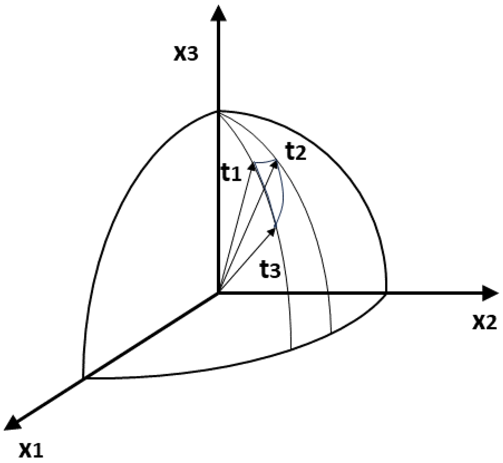
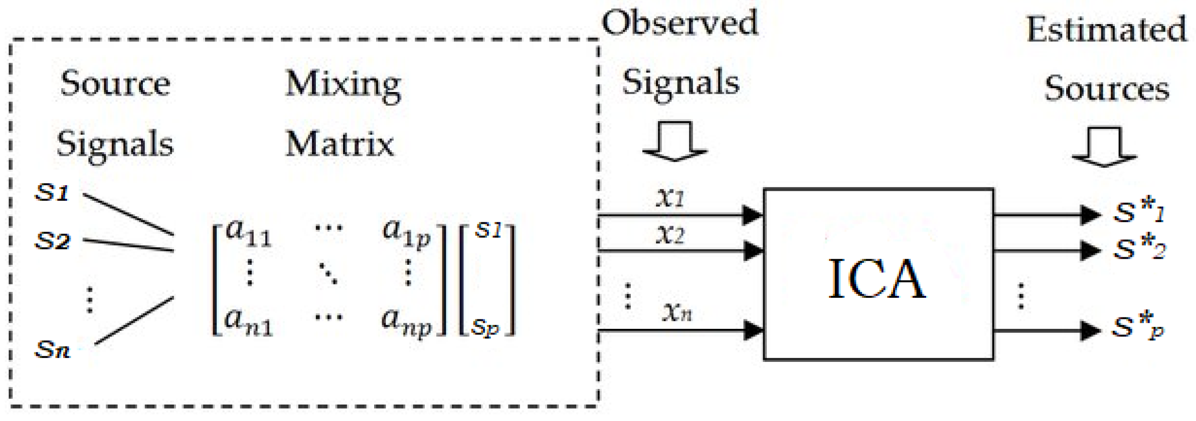
6.5. Independent Component Analysis and Blind Source Separation

PCA is a variance-based representation and is a low rank approximation by taking the k largest eigenvectors associated with their corresponding eigenvalues. ICA provides a measure of independence other than variance, which is useful when the data (signals) depend on time. The non-existence of correlation means independence only if variables (column normalized matrix $\mathbf{X}$) are Gaussian, but not in other cases. ICA is introduced to help in such situations. The objective is to separate observations into the underlying signals. Figure 5 explains this idea.

In this case, the matrix $\mathbf{X}$ is transformed as

$$\begin{array}{c}\hfill \mathbf{S}=\mathbf{B}\mathbf{X}\end{array}$$

(70)

where $\mathbf{B}$ is a basis. An approximation is obtained by minimizing a divergence between $\mathbf{S}$ and the column-normalized matrix $\mathbf{Y}$.

Minor components are associated with noise. A set of techniques known as Blind source separation (BSS) exists to extract them. This approach assumes the consideration of dynamic systems, in which the entries $\mathbf{X}=\mathbf{X}\left(t\right)$ are time-dependent (t is time) and centered. The classic approach, attributed to Oja [156], supposes an update of the matrix $\mathbf{W}={(w_1,\dots ,w_m)}^{\prime }$ with the update rules

$$\begin{array}{c}\hfill \mathbf{W}\left(t\right)=\mathbf{W}(t-1)+\gamma \left(t\right)\mathbf{x}\left(t\right)\mathbf{x}{\left(t\right)}^{\prime }\mathbf{W}(t-1)\end{array}$$

(71)

where $\gamma \left(t\right)$ is a scalar representing the gain parameter, $\mathbf{x}\left(t\right)$ the systems inputs, and $\mathbf{W}$ are the constraints to maximize $E\left({\mathbf{w}}_i^{\prime }\mathbf{x}\right)$, subject to orthogonality.

Orthonormalizing the expression (71) by introducing a suitable array $\mathbf{S}\left(t\right)$

$$\begin{array}{c}\hfill {\mathbf{W}}_{\perp }\left(t\right)=\mathbf{W}\left(t\right)\mathbf{S}{\left(t\right)}^{-1}\end{array}$$

(72)

${\mathbf{W}}_{\perp }\left(t\right)$ is an orthonormal matrix.

Taking into account that the product $\mathbf{x}\left(t\right)\mathbf{x}{\left(t\right)}^{\prime }$ is the covariance matrix, which is represented now as $\mathbf{V}$, the differential equations corresponding are obtained by simple differentiation of (72)

$$\begin{array}{cc}\hfill \dot{\mathbf{W}}& \hfill =\mathbf{X}{\mathbf{X}}^{\prime }\mathbf{W}-\mathbf{W}{\mathbf{W}}^{\prime }\mathbf{X}{\mathbf{X}}^{\prime }\mathbf{W}\hfill \end{array}$$

(73)

$$\begin{array}{cc}\hfill & \hfill =\mathbf{V}\mathbf{W}-\mathbf{W}{\mathbf{W}}^{\prime }\mathbf{V}\mathbf{W}\hfill \end{array}$$

(74)

The dot means, as usual, the time derivative. It is stable in the Lyapunov sense (a linear combination nearby solution differs from a first-order infinitesimal).

Further studies by Chen [157] established that the necessary and sufficient condition to extract the principal space (principal components) is that the initial condition $\mathbf{W}\left(0\right)$ must be full rank. In this case, it occurs that

$$\begin{array}{c}\hfill \mathbf{W}\left(t\right)\underset{t\to \infty }{\to }\mathbf{W}\end{array}$$

(75)

and introducing $\mathbf{W}=\theta \mathbf{D}$ ($\mathbf{D}$ is diagonal) to orthogonalize, we have

$$\begin{array}{c}\hfill \dot{\mathbf{W}}=\mathbf{V}\mathbf{W}\mathbf{D}-\mathbf{W}{\mathbf{W}}^{\prime }\mathbf{V}\mathbf{W}\end{array}$$

(76)

in this case, the SVD of $\mathbf{W}$ takes the form

$$\begin{array}{c}\hfill \mathbf{W}\left(t\right)=\mathbf{U}\left(t\right)\mathbf{D}\left(t\right)\mathbf{V}\left(t\right)\end{array}$$

(77)

with invariance properties for $\mathbf{U}$, $\mathbf{D}$, and $\mathbf{V}$ in (77) [154], p. 321.

A more recent approach focused on detecting minor components, with illustrative examples, is that by Tan [158].

Related BSS methods have grown remarkably since the formulation of pioneering studies by Oja [156] and Chen [157], finding applications in physics, engineering, finance, and medicine, among many others. Without being unfair to the many excellent published studies, we highlight the one by Cichocki, applicable when the dimensionality of the latent variable space is unknown [159].

The construction of matrix (77) is used in the PLSA sense in [160] with a non-negative probabilistic decomposition of the spectra components. In addition, the author reports that the method is better than PCA. A study in the area of IR combining both techniques is [161], reporting better and more accurate results than those obtained with ICA.

6.6. Transfer Learning

Transfer learning can be defined as the machine learning problem of trying to transfer knowledge from a source domain to a target domain [162].

PLSA can be used from the point of view of neural networks for TL purposes by solving the problem in the case in which the source domain shares only a subset of its classes (column vectors of the data matrix) for an unlabeled target data domain [21]. The log-likelihood expression is thus [21]

$$\begin{array}{cc}\mathcal{L}=\hfill & \hfill \sum _i\sum _{j}n(d_i^S,w_j)log\sum _i\sum _{j}P\left(d_i^S\right|z_k^S)P\left(w_j\right|z_k^S)P\left(z_k\right|z_k^S)\hfill \end{array}$$

$$\begin{array}{cc}\hfill & \hfill +\sum _i\sum _{j}n(d_i^T,w_j)log\sum _i\sum _{j}P\left(d_i^T\right|z_k^T)P\left(w_j\right|z_k^T)P\left(z_k\right|z_k^T)\hfill \end{array}$$

(78)

where S indicates that a document is in the source, and T indicates the target domain. A detailed survey introducing neural networks is [163]. A similar study on the issue of TL was carried out by [164].

Krithara reports that TL with PLSA seems particularly effective for multiclass text classification tasks with many classes and few documents per class, and the performance is better than other methods when the percentage of shared classes of source and target domain is small. Ref. [165] detects changes and anomalies in high-dimensional data. Ref. [166] analyzes purchase behavior.

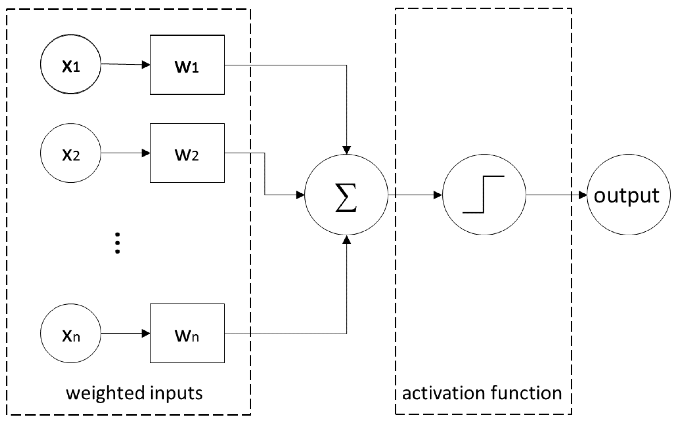
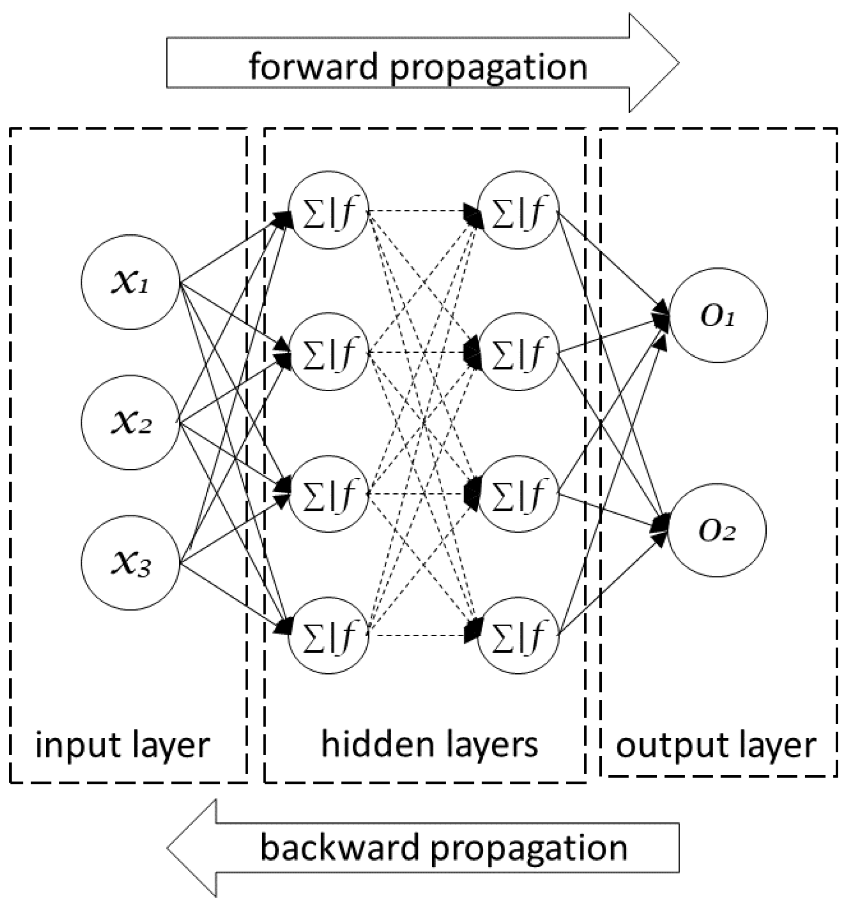
6.7. Neuronal Networks

Neural networks (NN) are a set of techniques based on the idea of the perceptron, a mathematical entity that simulates the behavior of a biological neuron [167]. The fundamental idea is to create computational systems using its characteristics that consist of weighing several input signals and activating the output if a cut value is exceeded. A simplified model for the j-th neuron is

$$\begin{array}{cccc}\hfill & \mathrm{input}\mathrm{signals}:\hfill & \hfill & x_i\left(t\right)\hfill \\ \hfill & \hfill \mathrm{weight}\mathrm{of}\mathrm{input}\mathrm{signals}:\hfill & \hfill & w_i\hfill \end{array}$$

with output

$$\begin{array}{c}\hfill f\left(t\right)=f\left(\sum _i{w}_i{x}_i\left(t\right)\right)\end{array}$$

(79)

with f being an activation function known as the sigmoid function (a function that leads to an output if the input is greater than a predetermined value, and zero otherwise). The model is illustrated in Figure 6. Ref. [168] provides an introduction to the types of such functions and their effects on the output, and Ref. [169] offers a more recent study on this topic.

The limitations of a simple perceptron model lead to multilayer architectures, an idea by to [170]. The standard multilayer model or $L-$ layer assumes the existence of $L-1$ hidden layers and an output layer. Conventionally, the input layer is omitted. A multilayer model is shown in Figure 7. The multilayer model can be constructed by superpositioning the single perceptrons, and

$$\begin{array}{c}\hfill f_j\left(t\right)=f\left(\sum _i\mathbf{W}\left(t\right)x_i\left(t\right)\right)\end{array}$$

(80)

To apply the model, it is necessary to know what information is available and how to update the weights. The model is trained to minimize the objective function, for which several techniques exist, like the backward propagation error.

A strategy is to minimize the error function

$$\begin{array}{c}\hfill {\mathbf{W}}_i\left(t\right)x_i\left(t\right)=\frac{exp\left(-\mathbf{W}\left(t\right)x_i\left(t\right)F_i\right)}{{\sum }_i{F}_i}\end{array}$$

(81)

where $F_i=f({\sum }_i\mathbf{W}\left(t\right)x_i\left(t\right)$. A quick introduction to this topic is the classic tutorial by [171], while a classic exposition is presented by [172].

Although NN methods are deterministic, probabilistic approaches can be used when there is uncertainty in the data and justification to use the PLSA. The introduction of the PLSA in this field is attributed to [22]. The basic idea is first to adjust the probabilities of the relation (3) and to simplify the notation take the vectors ${\mathbf{x}}_j=P\left(w_j\right|d_i)$; and ${\mathbf{y}}_j=P\left(w_j\right|z_k)$. In this case, f takes the form

$$\begin{array}{c}\hfill f_j=\frac{exp\left\{{\sum }_i{\mathbf{y}}_j{\mathbf{x}}_j\right\}}{{\sum }_{i}exp\left\{{\sum }_i{\mathbf{y}}_j{\mathbf{x}}_j\right\}}\end{array}$$

(82)

and not depending on the time.

Ba’s work showcases research expertise; however, it occasionally leaves certain details for the reader to infer. Conversely, the sigmoid function tends to smooth the probabilities, which creates problems in choosing cut-off values.

6.8. Open Questions

Gaussier and Ding’s studies have been important in relating the PLSA and the SVD, translating the conceptual framework to the context of the probabilistic interpretations of the NMF, extending the data class domain from the non-negative integers to the non-negative reals, and relaxing distributional assumptions, since no hypothesis is conducted on the parameter space. This is a non-parametric method based on NMF algebra. In addition, NMF techniques mainly focus on symmetric formulation. There does not seem to be any objection preventing its use for the asymmetric one, although problems in assigning probabilities $P\left(d_i\right)$ in Equation (2) could complicate the problem.

In addition, Ding has stated that the difference between the results of the SVD and NMF (and, thus, PLSA) depends on the convergence to different local optima, and it is true if $k<min(m,n)$. Ding’s studies have considered SVD as a dimensional reduction problem or low-rank decomposition. In this case, the matrix $\mathbf{WH}$ will not be $\mathbf{Y}$, but an approximation, and the SVD is not achievable with NMF. In addition, because PCA decomposition is related to the geometric multiplicities of eigenvalues, in the case of the relations obtained with NMF, it is not so clear, and it should be faced with algebraic dimensionality (PCA dimension refers to the geometric multiplicity of the eigenvalues ${\sigma }_r$ of the SVD theorem and corresponds to $dimE\left(\sigma \right)$, with $E\left(\sigma \right)=\{\mathbf{v}\in {\mathbb{R}}^m\mathrm{s}.\mathrm{t}\mathbf{Y}{\mathbf{v}}_r=\sigma {\mathbf{u}}_y\}$ being ${\mathbf{u}}_r$ and ${\mathbf{v}}_r$ vectors of $\mathbf{U}$ and $\mathbf{V}$, respectively. The nonzero roots of $\sigma$, such that $det(\mathbf{Y}-\sigma \mathbf{I})=0$, referred to as the characteristic polynomial, represent the algebraic multiplicity. Both concepts play a fundamental role in the canonical forms [173], Chapter 10, and are crucial for interpreting dimensionality in matrix analysis).

However, when the discussion is restricted to the symmetric formulation, questions arise, and the results depend on k and determining the equivalence of the solutions, leaving aside the type of convergence of $\mathbf{WH}\to \mathbf{Y}$, which holds in the case $k\ge min(m,n)$, as indicated by several authors [16,19,174]. Suboptimality occurs when this condition is not fulfilled and implies that the SVD low-rank approximation is an ill-conditioned problem [19].

7. PLSA Processing Steps and State-of-the-Art Solutions

PLSA is considered an effective technique but has a notable drawback in its high consumption of computing resources, in terms of both execution and internal memory. This drawback has limited its practical applications [175] and additionally makes the relationship between the SVD and PLSA curious. In the SVD case, the typical blackboard exercise of obtaining eigenvalues and eigenvectors is simple but does not occur similarly for moderate and large datasets. Methods for its effective computation have arisen from numerous studies and sustained efforts over several decades [176]. Currently, many language programs implement the Linear algebra package (LAPACK) to facilitate SVD computation [177]. Also, solutions for PLSA are hard to obtain.

Beyond the EM algorithm problems, PLSA is highly dependent on the initialization values [178,179]. This leads to several algorithms for computational efficiency purposes, based on certain initialization conditions, and others on alternative versions of the EM algorithm, apart from those that strictly use computational techniques.

Herein, contributions to increasing computational efficiency are examined according to the concepts on which they are based, their initialization conditions, and the use of EM algorithm variants. Efforts using purely computational techniques are also discussed.

7.1. Algorithm Initialization

The dependence of the PLSA results on the initialization conditions has led to several variations. One possibility, applicable only in the symmetric formulation, as proposed by [178], initializes the algorithm with LSA solutions, which are the SVD solutions. Because some values can be negative, correction may be necessary (typically setting values to zero). Another strategy applicable in both formulations is execution for several random initialization distributions of the considered algorithm; after running, the higher log-likelihood value offers the best solution [179].

One algorithm is Online belief propagation (OBP), which is based on a sequence of initializations on subsets of the data frame [179,180]. OBP segments the data frame into several parts. After the initialization of the first segmentation, solutions are obtained and used in the next initialization, and so on. This technique enables the use of PLSA on large datasets.

A fundamental of the OBP is stochastic initialization [181], which consists of defining a learning function as a risk function for which the difference in conditional distributions describes a decreasing sequence between iterations [181]. The execution of this algorithm requires at least one iteration for the complete dataset and the selection of the most significant contributions to the first partition.

In [182], it is reported that algorithms based on these principles present advantages over other existing algorithms for IR in the context of big data and for determining parameters in sets of data streams without ending. This procedure has been advantageously applied in automatic translation with a topic model obtained from the LSA and a subsequent adjustment with the PLSA [183]. However, these claims should be re-examined. The LDA represents the SVD, which presents serious computational problems with large data structures [129], giving rise to several approaches, such as randomized SVD, kernelization methods, and the CUR method, consisting of extracting a matrix C into a lower-dimensional space (for rows and columns) and using a compressed representation of the data, or a sample, obtaining the truncated SVD.

7.2. Algorithms Based on Expectation–Maximization Improvement

The EM convergence rate is [184]

$$\begin{array}{c}\hfill \parallel {\theta }^{(p+1)}-{\theta }^{★}\parallel \le \lambda \parallel {\theta }^{\left(p\right)}-{\theta }^{★}\parallel \end{array}$$

(83)

where $\lambda$ is the largest eigenvalue of the data matrix. Several methods are used to accelerate convergence, such as the descendant gradient. However, PLSA must preserve maximum log-likelihood solutions. To improve computational efficiency in such conditions, some variants and alternative algorithms have been proposed. The EM algorithm is one of the most studied in statistical environments, and many variants and simplifications exist [185]. The EM algorithm is the classic optimization technique for PLSA, and some versions or modifications have been exploited to achieve PLSA solutions. A general description of the algorithm used in this section is [186].

7.2.1. Tempered EM

Tempered EM uses classical concepts of statistical mechanics for computational purposes [187]. Aside from the significance in physics, the primary idea is achieving a posterior (E-step) close to a uniform distribution. An objective function is introduced

$$\begin{array}{cc}\hfill {\mathcal{F}}_{\beta }& \hfill =-\beta \sum _i\sum _{j}n(d_i,w_j)\sum _k\tilde{P}(z_k;d_i,w_j)log\left[P\left(d_i\right|z_k)P\left(w_j\right|z_k)P\left(z_k\right)\right]\hfill \end{array}$$

$$\begin{array}{cc}\hfill & \hfill +\sum _i\sum _{j}n(d_i,w_j)\sum _k\tilde{P}\left(z_k\right|d_i,w_j)logP\left(z_k\right|d_i,w_j)\hfill \end{array}$$

(84)

where $\tilde{P}(z_k;d_i,w_j)$ is a variational parameter defined as

$$\begin{array}{c}\hfill \tilde{P}(z_k;d_i,w_j)=\frac{{\left[P\left(z_k\right)P\left(d_i\right|z_k)P\left(w_j\right|z_k)\right]}^{\beta }}{{\sum }_k{\left[P\left(z_k\right)P\left(d_i\right|z_k)P\left(w_j\right|z_k)\right]}^{\beta }}\end{array}$$

(85)

and for $\beta <1$, the convergence is faster [17].

7.2.2. Sparse PLSA

A proposal to improve the convergence speed has been based on sparse EM [188]. Assuming that only a subset of values is plausible for latent variables (in terms of probabilities), freezing non-significant avoids many calculations. PLSA is considered to be an algebraic optimization problem of the matrix $\mathbf{Y}\in {\mathbb{R}}^{m\times n}$ (which in this case is the data frame containing the relative frequencies $n(d_i,w_j)$) restricted to the constraint ${\sum }_r{\lambda }_r{\mathbf{y}}_r{\mathbf{y}}_r^t(r<m)$, or unknown parameters, minimizing [189]

$$\begin{array}{c}\hfill D_q(\mathbf{Y}\parallel \sum _r{\lambda }_r{\mathbf{y}}_r{\mathbf{y}}_{r^{\prime }})(\mathrm{with}\sum _r{\lambda }_r=\parallel {\mathbf{y}}_r{\parallel }_1=\parallel {\mathbf{y}}_r^{\prime }{\parallel }_1=1,{\mathbf{y}}_r\in \mathbf{Y}\mathrm{and}{r}^{\prime }\ne r<n)\end{array}$$

(86)

named Tsallis divergence [190], and computed for the r non-freezing column vectors of $\mathbf{Y}$ as [57], p. 97

$$\begin{array}{c}\hfill D_q({\mathbf{y}}_j\parallel {\lambda }_r{\mathbf{y}}_r{\mathbf{y}}_r^t)=\frac{1}{\kappa }\sum _i\left({\mathbf{y}}_j\left({\mathbf{y}}_j^{\kappa }-{\left({\lambda }_r{\mathbf{y}}_r{\mathbf{y}}_r^t\right)}^{\kappa }\right)\right)-\sum _i\left({\mathbf{y}}_j^{\kappa }\left({\mathbf{y}}_j-{\lambda }_r{\mathbf{y}}_r{\mathbf{y}}_r^t\right)\right)(\mathrm{s}.\mathrm{t}.\kappa \ne 0)\end{array}$$

(87)

This divergence solves the optimization problem of adjusting $n(d_i,w_j)$ to $P(d_i,w_j)$ [191]. After adjustment, probabilistic factorizations of the considered parametrization must again be obtained.

7.2.3. Incremental PLSA

Instead of global maximization, simpler contributions can be maximized. This update procedure used in the E-step for the PLSA gave rise to the incremental PLSA algorithm [192], with which results can be obtained twice as quickly. Applications in image classification can be found in [193,194].

A recursive algorithm, called recursive probabilistic latent semantic analysis, is based on the computation of the likelihood of a subset of words, as well as other words, recursively [195]. The performance has been reported to be highly similar to that obtained with the incremental PLSA.

7.3. Use of Computational Techniques

Difficulties obtaining fast and reliable solutions for PLSA have also been approached through purely computational techniques. These advancements are a consequence of developments in computer architecture in recent decades: processing capabilities have been increased, thus resulting in a new branch of algorithms to reduce the computational time of the PLSA. The introduction of multicore processors by Intel and Sun Microsystems in 2005 for portable machines enabled a major step toward parallel computing [196], which is now the dominant paradigm.

Parallel computing involves the simultaneous execution of tasks. It requires dividing a problem into independent pieces and executing each one in a separate processing unit. The use of parallel computing techniques for the PLSA has been proposed in [197]. A current and widespread technique to support parallel capabilities is Map Reduce [198]. This technique essentially consists of dividing tasks into two phases. The first phase is a map that partitions the input dataset and assigns labels to each one. The reduce phase supposes the execution of an operation on a set of previously labeled partitions. An algorithm exploiting the possibilities of Map Reduce for the PLSA results has been proposed in [199]. Also, it reports problems due to the limited memory [199]. A recent application for the effectiveness of research and development is largely determined by the application of the best achievements in science and technology. To find and select the best solutions, experts conduct patent searches in databases containing up to tens of millions of documents. In existing systems, documents are searched for by keywords. The complexity of performing patent searches in existing systems is due to the large number of documents matching the search query. The authors have developed a methodological approach to automating the structuring of the patent research results, based on thematic modeling of a collection of documents obtained as a result of a keyword search query [200].

Furthermore, graphic processing units have increased the range of capabilities, and they are useful for a broad variety of applications, particularly the simulation of complex models (General-Purpose Computation Graphics Hardware at https://web.archive.org/web/20051214111850/http://www.gpgpu.org/ (accessed on 31 March 2023). These capabilities have been transferred to the PLSA algorithm [201]. Ref. [202] provides a new parallel version of Statistical dual-depth sparse probabilistic latent semantic analysis (DEpLSA), reporting significant acceleration, but it has not yet produced definitive results.

7.4. Open Questions

The described methods do not provide completely satisfactory results, and perhaps it is one of the causes of the division between enthusiasts and indifferent regarding PLSA. The PLSA algorithms inherit the problems of EM, especially the slow convergence. Surprisingly, despite the EM algorithm being one of the most studied, many versions and works have been devoted to accelerating convergence (a recent one is [203]), but there are no comparative studies.

Our research suggests that initializing Formulas (37a)–(37c) with the SVD and jittering, few iterations using parallel computing techniques produce good results, at least for moderate-sized datasets.

8. Future Work

The first question that arises is about the nature of the data. According to [12], the use of NMF techniques seems to reduce them to statistical independence (In the examples made in [204], we built a method for clustering validation with the probabilistic images of the data with no restrictions on the class. This method consists of taking the linearly independent columns of (35) and then varying the dimensionality of the space span, the sequence

$$\begin{array}{cc}\hfill z_k& \hfill ={\left\{tr{\left({\left[\mathbf{W}\right]}_{ik}{\left[\mathbf{H}\right]}_{kj}\right)}^t\left({\left[\mathbf{W}\right]}_{i1}{\left[\mathbf{H}\right]}_{1j}\right)\right\}}_{k=1}^{\infty }\hfill \end{array}$$

The expectation of the limit of this sequence is a gamma distribution, and it reasonably coincides with the values of the Silhouette index and gap statistic. In the experiments we conducted, for the dataset glass of the repository https://archive.ics.uci.edu/datasets (accessed on 15 February 2022), we take the iid and omit two columns that can be considered as Boolean variables, indicating special chemical treatments. Introducing this variable, the number of clusters is doubled, suggesting that the method can capture and model with the hypothesis of independent variables). However, this statement requires further studies and comparatives and it is faced with important overlapping cases.

The other question is on transformation to the probability domain. It involves the construction of a probabilistic matrix that can be assimilated into a random variable. Formally, it can be justified to fix a value for j and consider the matrix as a juxtaposition of column vectors. This construction is consistent with the estimation of a density $f_j$ associated with the distribution P that generates the data [62], Chapter 1. It has been discussed in Section 3.2.5 that this transformation, when performed according to Laplace’s rule in Hofmann’s original formulation, is also equivalent to smoothing with a triangular kernel. This choice provides similar results and is equivalent to any other choice in which the minimization of some variance function would provide different values of the smoothing parameter h. In these cases, the results would only be equivalent, but in no case similar. We point out that there are other transformations. Among them is the logistic transformation $\varphi \left(\mathbf{X}\right)=1/(1+exp(\mathbf{X}\left)\right)$, which is used in regression problems to relate the response and the explanatory variables. In the case of proportions, it has been widely used to avoid the concentration of values at the ends of the range, and provides good results in the tails of the distribution. This transformation can be understood as a sigmoid-type transformation [169]. These transformations should be explored in the context of PLSA.

This situation could be used to advance in the context of Big Data. It would simply involve smoothing the data matrix to use the approximation

$$\begin{array}{c}\hfill \mathrm{MISE}\left(\widehat{f}\right)=E{\left\{{\int }_{\mathcal{D}}(\widehat{f}-f)dx\right\}}^2\end{array}$$

where Mean integrated standard error (MISE) is the global variance, as explained in the referred book [63], f is the data image, and $\widehat{f}$ is its estimation. Using this definition in the reverse sense (i.e., a parametric distribution is fitted to the smoothed function) can save computational efforts. Then, the information geometry methods (considering the similarity or distance between densities in the parameter space) would provide a great operational advantage. We emphasize that this is how Rao formulated the problem when he faced massive data [148,149]. The parameter space is often of reduced dimension.

The practical problems that he presents as anIR technique are difficult to solve. Among these problems are polysemy and synonymy. These problems have solutions in the LDA context and have led some researchers and practitioners to consider the PLSA as an obsolete method. However, these methods based on LDA and described in Section 3.1 also suffer an important drawback: their statistical properties are not clear, while PLSA provides maximum likelihood solutions.

The symmetric formulation of the PLSA provides a rich interpretive framework. It allows the formulation of the PLSA as a multivariate technique in which the transformation to and the use of NMF techniques alleviates several problems. Using the EM algorithm to adjust probabilities provides a maximum likelihood estimation of the parameters. This result can be generalized to other divergences. In particular, Bregman divergence allows a generalization of these results as shown in [205]. However, these methods preserving certain statistical properties are methods known as iterative updates. Other solutions, such as those provided by gradient descent methods, should be examined.

Convergence occurs for $k\ge min(m,n)$, however, for the case $k<min(m,n)$. Convergence problems described in Section 3 are due to the interpretation of the SVD and, therefore, the PCA as a low-rank approximation. However, these statements do not consider the low-rank approximation, based on Schmidt’s approximation Theorem [206]. Establishing a boundary with the help of this result is an open question.

The LDA techniques and those built on them are hierarchical models whose construction corresponds to particular fields of application. These constructions are also possible in the symmetric formulation assuming additional hypotheses on the data, like distribution, qualitative categories, or relations between categories or variables. This type of treatment supposes a pre-processing of the data, preserving the content of the PLSA significance.

Furthermore, although the concept of probabilistic learning is sound, based on Vaillant’s work [207], symmetric PLSA is especially apt in the context of TL. In this way, the certainty depends on the available data, as suggested by the relation (78). Then, reanalyzing a problem with new (or complementary) data or observational variables can provide learning sequences. Other lines of work, focused from a more practical point of view, would be the construction of ICA with the PLSA model, relating it to the PCA in the probabilistic context; TL with the same hypotheses; and their use in neural networks and depend solely on the imagination of the researcher or practitioner. Asymmetric formulation, currently a mere IR technique, should be explored in the same sense, except in the PCA case.

9. Discussion

The period of most significant growth for PLSA can be identified as the decade from 2005 to 2015, marking the beginning of its maturation and its end with limitations, especially computational ones, revealed mainly in bioinformatics, typically requiring massive data processing, against which, traditionally, the PLSA has shown its weakness. To this, we must add the continuously exponential growth of the web. It is during this period that more than half of the works that used techniques related to the PLSA received support from some founding agency ($55\%$ according to our queries in Web of Science).

This situation—in which solutions take priority and their attainment is conditioned by the need for them to be in real-time—reflects the current dominant paradigm in the science of a positivist orientation [208]: the cumulative addition of works. Without criticizing the numerous contributions of this orientation, we note that it has overshadowed many of the works referenced in Section 6. This observation demonstrates that the PLSA, especially in its symmetric formulation, can lay the foundation for other techniques and can be utilized in most operating system (OS! (OS!)) machine learning (ML) scenarios.

Another consequence, perhaps unnoticed, of the positivist current, is the admission of simple verifications as a demonstration of the quality of a technique (and these are the typical numerical experiments that appear at the end of many publications). In fundamental sciences, experimentation is used to validate or refute hypotheses. They evaluate the relationship or dependence between causes and their effects (except in the fields of relativistic mechanics, in which the situation is somewhat more complicated), and not the other way around. A consequence, expressed explicitly in the context of clustering validation, is that the use of one or more criteria may inadvertently satisfy different algorithms [39], p. 22. This way of thinking works against well-sound methods, such as PLSA. Furthermore, the appearance of many alternative techniques brings to mind the conceptual complexity that the celestial mechanics of the Ptolemaic system endured with the successive introduction of equants, until the great simplification brought about by Galileo. Baroque complexity has never been conducive to the advancement of science. The abuse of hierarchical models in ML is baroque.

On the other hand, the results provided by the PLSA allow the interpretation of the structure of the data in the space of latent variables in all the application areas with satisfactory results. In addition, it shares with the SVD the computational problems faced with large data structures.

Furthermore, issues related to the interpretability and explainability of ML methods have recently gained ground. We believe that the PLSA (in its symmetric formulation and as a probabilistic image of the SVD) can be of help in these questions. The SVD is the starting point of many branches of pure and applied mathematics, such as eigenanalysis and integral equations, and can find its companion in the PLSA in cases where the data present uncertainty.

From this point of view, the PLSA represents a paradigm. Its development can offer an explanatory framework from which many other techniques can be better understood, also providing a broad spectrum of applications that appear to have no limit.

10. Conclusions

The PLSA is a technique with a quarter-century of existence and has been applied to many research areas with good results. Despite the formal equivalence of the formulations, the asymmetric formulation is an IR technique, while the symmetric formulation also allows for establishing a probabilistic relationship with the SVD. Consequences of this relationship include laying the foundation for the probabilistic construction of other techniques, such as kernelization, PCA, clustering, or TL, as well as the possibility of building a Fisher kernel. However, there are some open questions, notably the approximation error when using the low-rank approximation and poor computational efficiency.

The computational problems of PLSA have limited its diffusion, although algorithms based on NMF alleviate this problem. Furthermore, these algorithms preserve statistical or geometric properties. From a practical perspective, the PLSA allows the construction of Fisher kernels, the probabilistic interpretation of PCA, applications in TL, and the training of neural networks. On the other hand, the formulation from the NMF also plays a significant role. These results lead to the conclusion that the PLSA offers a valuable opportunity for theoretical research. From a purely practical standpoint, it finds applications in many areas, offering notable advantages.

References

1. Hofmann, T. Probabilistic latent semantic indexing. In Proceedings of the 22nd Annual International ACM SIGIR Conference on Research and Development in Information Retrieval, Berkeley, CA, USA, 15–19 August 1999. [Google Scholar]
2. Hofmann, T. Probabilistic latent semantic analysis. In Proceedings of the Uncertainty in Artificial Intelligence, Eindhoven, The Netherlands, 1–5 August 1999. [Google Scholar]
3. Hofmann, T. Unsupervised learning by probabilistic latent semantic analysis. In Machine Learning; Springer: Berlin/Heidelberg, Germany, 2001. [Google Scholar]
4. Deerwester, S.; Dumais, S.T.; Furnas, G.W.; Landauer, T.K.; Harshman, R. Indexing by latent semantic analysis. J. Am. Soc. Inf. Sci. 1990, 41, 391–407. [Google Scholar] [CrossRef]
5. Saul, L.; Pereira, F. Aggregate and mixed-order Markov models for statistical language processing. arXiv 1997, arXiv:cmp-lg/9706007. [Google Scholar]
6. Barde, B.V.; Bainwad, A.M. An overview of topic modeling methods and tools. In Proceedings of the 2017 International Conference on Intelligent Computing and Control Systems (ICICCS), Madurai, India, 15–16 June 2017; pp. 745–750. [Google Scholar]
7. Ibrahim, R.; Elbagoury, A.; Kamel, M.S.; Karray, F. Tools and approaches for topic detection from Twitter streams: Survey. Knowl. Inf. Syst. 2018, 54, 511–539. [Google Scholar] [CrossRef]
8. Tian, D. Research on PLSA model based semantic image analysis: A systematic review. J. Inf. Hiding Multimed. Signal Process. 2018, 9, 1099–1113. [Google Scholar]
9. Brants, T. Test data likelihood for PLSA models. Inf. Retr. 2005, 8, 181–196. [Google Scholar] [CrossRef]
10. Masseroli, M.; Chicco, D.; Pinoli, P. Probabilistic latent semantic analysis for prediction of gene ontology annotations. In Proceedings of the 2012 International Joint Conference on Neural Networks (IJCNN), Brisbane, Australia, 10–15 June 2012; pp. 1–8. [Google Scholar]
11. Hofmann, T. Collaborative filtering via gaussian probabilistic latent semantic analysis. In Proceedings of the 26th Annual International ACM SIGIR Conference on Research and Development in Informaion Retrieval, Toronto, ON, USA, 28 July–1 August 2003; pp. 259–266. [Google Scholar]
12. Figuera, P.; García Bringas, P. Non-Parametric Nonnegative Matrix Factorization Fisher Kernel. SSRN 2023, 4585853. [Google Scholar] [CrossRef]
13. Tar, P.D.; Thacker, N.A.; Deepaisarn, S.; O’Connor, J.; McMahon, A. A reformulation of pLSA for uncertainty estimation and hypothesis testing in bio-imaging. Bioinformatics 2020, 36, 4080–4087. [Google Scholar] [CrossRef]
14. Gaussier, E.; Goutte, C. Relation between PLSA and NMF and implications. In Proceedings of the 28th Annual International ACM SIGIR Conference on Research and Development in Information Retrieval (SIGIR’05), Virtual, 11–15 July 2005. [Google Scholar]
15. Ding, C.; He, X.; Simon, H.D. On the equivalence of nonnegative matrix factorization and spectral clustering. In Proceedings of the 2005 SIAM international conference on data mining (SIAM), Newport Beach, CA, USA, 21–23 April 2005; pp. 606–610. [Google Scholar]
16. Figuera, P.; García Bringas, P. On the Probabilistic Latent Semantic Analysis Generalization as the Singular Value Decomposition Probabilistic Image. J. Stat. Theory Appl. 2020, 19, 286–296. [Google Scholar]
17. Hofmann, T. Learning the similarity of documents: An information-geometric approach to document retrieval and categorization. In Proceedings of the Advances in Neural Information Processing Systems, Denver, CO, USA, 2000; pp. 914–920. [Google Scholar]
18. Chappelier, J.C.; Eckard, E. Plsi: The true fisher kernel and beyond. In Proceedings of the Joint European Conference on Machine Learning and Knowledge Discovery in Databases, Bled, Slovenia, 7–11 September 2009; Springer: Berlin/Heidelberg, Germany, 2009; pp. 195–210. [Google Scholar]
19. Klingenberg, B.; Curry, J.; Dougherty, A. Non-negative matrix factorization: Ill-posedness and a geometric algorithm. Pattern Recognit. 2009, 42, 918–928. [Google Scholar] [CrossRef]
20. Chaudhuri, A.R.; Murty, M.N. On the Relation Between K-means and PLSA. In Proceedings of the 2012 21st International Conference on Pattern Recognition, Tsukuba, Japan, 11–15 November 2012. [Google Scholar]
21. Krithara, A.; Paliouras, G. TL-PLSA: Transfer learning between domains with different classes. In Proceedings of the 2013 IEEE 13th International Conference on Data Mining, Dallas, TX, USA, 7–10 December 2013; pp. 419–427. [Google Scholar]
22. Ba, S. Discovering topics with neural topic models built from PLSA assumptions. arXiv 2019, arXiv:1911.10924. [Google Scholar]
23. Blei, D.M.; Ng, A.Y.; Jordan, M.I. Latent Dirichlet Allocation. J. Mach. Learn. Res. 2003, 3, 993–1022. [Google Scholar]
24. Ding, C.H.; Li, T.; Jordan, M.I. Convex and semi-nonnegative matrix factorizations. IEEE Trans. Pattern Anal. Mach. Intell. 2008, 32, 45–55. [Google Scholar] [CrossRef] [PubMed]
25. Devarajan, K.; Wang, G.; Ebrahimi, N. A unified statistical approach to non-negative matrix factorization and probabilistic latent semantic indexing. In Machine Learning; Springer: Berlin/Heidelberg, Germany, 2015. [Google Scholar]
26. Vangara, R.; Bhattarai, M.; Skau, E.; Chennupati, G.; Djidjev, H.; Tierney, T.; Smith, J.P.; Stanev, V.G.; Alexandrov, B.S. Finding the number of latent topics with semantic non-negative matrix factorization. IEEE Access 2021, 9, 117217–117231. [Google Scholar] [CrossRef]
27. Hong, L. A tutorial on probabilistic latent semantic analysis. arXiv 2012, arXiv:1212.3900. [Google Scholar]
28. Dempster, A.; Laird, N.; Rubin, D. Maximum Likelihood from Incomplete Data via the EM Agorithm. J. R. Stat. Soc. Ser. Methodol. 1977, 39, 1–22. [Google Scholar]
29. Jebara, T.; Pentland, A. On reversing Jensen’s inequality. In Proceedings of the Advances in Neural Information Processing Systems, San Francisco, CA, USA, 30 November–3 December 2001; pp. 231–237. [Google Scholar]
30. Wu, C.J. On the convergence properties of the EM algorithm. Ann. Stat. 1983, 11, 95–103. [Google Scholar] [CrossRef]
31. Boyles, R.A. On the convergence of the EM algorithm. J. R. Stat. Soc. Ser. (Methodol.) 1983, 45, 47–50. [Google Scholar] [CrossRef]
32. Gupta, M.D. Additive non-negative matrix factorization for missing data. arXiv 2010, arXiv:1007.0380. [Google Scholar]
33. Archambeau, C.; Lee, J.A.; Verleysen, M. On Convergence Problems of the EM Algorithm for Finite Gaussian Mixtures. In Proceedings of the European Symposium on Artificial Neural Networks (ESANN), Bruges, Belgium, 23–25 April 2003; Volume 3, pp. 99–106. [Google Scholar]
34. Blei, D.M.; Lafferty, J.D. Dynamic topic models. In Proceedings of the 23rd International Conference on Machine Learning, Pittsburgh, PA, USA, 25–29 June 2006; pp. 113–120. [Google Scholar]
35. Girolami, M.; Kabǿn, A. On an equivalence between PLSI and LDA. In Proceedings of the 26th Annual International ACM SIGIR Conference on Research and Development In Informaion Retrieval, Toronto, ON, Canada, 28 July–1 August 2003. [Google Scholar]
36. Teh, Y.W.; Jordan, M.I.; Beal, M.J.; Blei, D.M. Hierarchical Dirichlet Processes. J. Am. Stat. Assoc. 2006, 101, 1566–1581. [Google Scholar] [CrossRef]
37. Mimno, D.; Li, W.; McCallum, A. Mixtures of hierarchical topics with pachinko allocation. In Proceedings of the 24th International Conference on Machine Learning, Corvalis, OR, USA, 20–24 June 2007; pp. 633–640. [Google Scholar]
38. Koltcov, S.; Ignatenko, V.; Terpilovskii, M.; Rosso, P. Analysis and tuning of hierarchical topic models based on Renyi entropy approach. arXiv 2021, arXiv:2101.07598. [Google Scholar] [CrossRef]
39. Aggarwal, C.C.; Clustering, C.R.D. Algorithms and Applications; CRC Press Taylor and Francis Group: Boca Raton, FL, USA, 2014. [Google Scholar]
40. Brants, T.; Chen, F.; Tsochantaridis, I. Topic-based document segmentation with probabilistic latent semantic analysis. In Proceedings of the Eleventh International Conference on Information and Knowledge Management, McLean, VA, USA, 4–9 November 2002; pp. 211–218. [Google Scholar]
41. Brants, T.; Tsochantaridis, I.; Hofmann, T.; Chen, F. Computer Controlled Method for Performing Incremental Probabilistic Latent Semantic Analysis of Documents, Involves Performing Incremental Addition of New Term to Trained Probabilistic Latent Semantic Analysis Model. U.S. Patent Number US2006112128-A1, 14 April 2006. [Google Scholar]
42. Zhuang, L.; She, L.; Jiang, Y.; Tang, K.; Yu, N. Image classification via semi-supervised pLSA. In Proceedings of the 2009 Fifth International Conference on Image and Graphics, Xi’an, China, 20–23 September 2009; pp. 205–208. [Google Scholar]
43. Niu, L.; Shi, Y. Semi-supervised plsa for document clustering. In Proceedings of the 2010 IEEE International Conference on Data Mining Workshops, Sydney, Australia, 13 December 2010; pp. 1196–1203. [Google Scholar]
44. Bosch, A.; Zisserman, A.; Muñoz, X. Scene classification via pLSA. In Proceedings of the European Conference on Computer Vision, Graz, Austria, 7–13 May 2006; Springer: Berlin/Heidelberg, Germany, 2006; pp. 517–530. [Google Scholar]
45. Hörster, E.; Lienhart, R.; Slaney, M. Continuous visual vocabulary modelsfor plsa-based scene recognition. In Proceedings of the 2008 International Conference on Content-Based Image and Video Retrieval, Niagara Falls, ON, Canada, 7–9 July 2008; pp. 319–328. [Google Scholar]
46. Li, Z.; Shi, Z.; Liu, X.; Shi, Z. Modeling continuous visual features for semantic image annotation and retrieval. Pattern Recognit. Lett. 2011, 32, 516–523. [Google Scholar] [CrossRef]
47. Ma, H.; King, I.; Lyu, M.R. Effective missing data prediction for collaborative filtering. In Proceedings of the 30th Annual International ACM SIGIR Conference on Research and Development in Information Retrieval, Amsterdam, The Netherlands, 23–27 July 2007; pp. 39–46. [Google Scholar]
48. Tian, D. Extended Probabilistic Latent Semantic Analysis for Automatic Image Annotation. J. Inf. Hiding Multim. Signal Process. 2017, 8, 903–915. [Google Scholar]
49. Shashua, A.; Hazan, T. Non-negative tensor factorization with applications to statistics and computer vision. In Proceedings of the 22nd International Conference on Machine Learning, Bonn, Germany, 7–11 August 2005; pp. 792–799. [Google Scholar]
50. Peng, W.; Li, T. On the equivalence between nonnegative tensor factorization and tensorial probabilistic latent semantic analysis. Appl. Intell. 2011, 35, 285–295. [Google Scholar] [CrossRef]
51. Harshman, R.A. Foundations of the PARAFAC Procedure: Models and Conditions for an Explanatory Multimodal Factor Analysis; University of California: Los Angeles, CA, USA, 1970. [Google Scholar]
52. Balažević, I.; Allen, C.; Hospedales, T.M. Tucker: Tensor factorization for knowledge graph completion. arXiv 2019, arXiv:1901.09590. [Google Scholar]
53. Yoo, J.; Choi, S. Probabilistic matrix tri-factorization. In Proceedings of the 2009 IEEE International Conference on Acoustics, Speech and Signal Processing, Taipei, Taiwan, 19–24 April 2009; pp. 1553–1556. [Google Scholar]
54. Sun, L.; Axhausen, K.W. Understanding urban mobility patterns with a probabilistic tensor factorization framework. Transp. Res. Part B Methodol. 2016, 91, 511–524. [Google Scholar] [CrossRef]
55. Zhang, M.; Chen, S.; Sun, L.; Du, W.; Cao, X. Characterizing flight delay profiles with a tensor factorization framework. Engineering 2021, 7, 465–472. [Google Scholar] [CrossRef]
56. Anisimov, A.; Marchenko, O.; Taranukha, V.; Vozniuk, T. Development of a semantic and syntactic model of natural language by means of non-negative matrix and tensor factorization. In Proceedings of the Text, Speech and Dialogue: 17th International Conference (TSD 2014), Brno, Czech Republic, 8–12 September 2014; Proceedings 17. Springer: Berlin/Heidelberg, Germany, 2014; pp. 324–335. [Google Scholar]
57. Cichocki, A.; Zdunek, R.; Amari, S.I. Nonnegative Matrix and Tensor Factorizations; John Willey and Sons Ltd.: Hoboken, NJ, USA, 2009. [Google Scholar]
58. Rodner, E.; Denzler, J. Randomized probabilistic latent semantic analysis for scene recognition. In Proceedings of the Iberoamerican Congress on Pattern Recognition, Guadalajara, Mexico, 15–18 November 2009; Springer: Berlin/Heidelberg, Germany, 2009; pp. 945–953. [Google Scholar]
59. Ho, T.K. The random subspace method for constructing decision forests. IEEE Trans. Pattern Anal. Mach. Intell. 1998, 20, 832–844. [Google Scholar] [CrossRef]
60. Kokonendji, C.C.; Senga Kiesse, T.; Zocchi, S.S. Discrete triangular distributions and non-parametric estimation for probability mass function. J. Nonparametric Stat. 2007, 19, 241–254. [Google Scholar] [CrossRef]
61. Senga Kiesse, T.; Cuny, H.E. Discrete triangular associated kernel and bandwidth choices in semiparametric estimation for count data. J. Stat. Comput. Simul. 2014, 84, 1813–1829. [Google Scholar] [CrossRef]
62. Balakrishnan, N.; Nevzorov, V.B. A Primer on Statistical Distributions; John Wiley & Sons: Hoboken, NJ, USA, 2004. [Google Scholar]
63. Bowman, A.W.; Azzalini, A. Applied Smoothing Techniques for Data Analysis: The Kernel Approach with S-Plus Illustrations; Oxford University Press: Oxford, UK, 1997; Volume 18. [Google Scholar]
64. Tao, Z.; Qi, Z.; Dequn, L. A Novel Probabilistic Latent Semantic Analysis Based Image Blur Metric. In Proceedings of the 2014 IEEE 12th International Conference on Dependable, Autonomic and Secure Computing, Dalian, China, 24–27 August 2014; pp. 310–315. [Google Scholar]
65. Murphy, L.; Sibley, G. Incremental unsupervised topological place discovery. In Proceedings of the 2014 IEEE International Conference on Robotics and Automation (ICRA), Hong Kong, China, 31 May–7 June 2014; pp. 1312–1318. [Google Scholar]
66. Wang, X.; Geng, T.; Elsayed, Y.; Ranzani, T.; Saaj, C.; Lekakou, C. A new coefficient-adaptive orthonormal basis function model structure for identifying a class of pneumatic soft actuators. In Proceedings of the 2014 IEEE/RSJ International Conference on Intelligent Robots and Systems, Chicago, IL, USA, 14–18 September 2014; pp. 530–535. [Google Scholar] [CrossRef]
67. Barbu, C.; Simina, M. A probabilistic information filtering using the profile dynamics. In Proceedings of the SMC’03 Conference Proceedings. 2003 IEEE International Conference on Systems, Man and Cybernetics. Conference Theme-System Security and Assurance (Cat. No. 03CH37483), Washington, DC, USA, 8 October 2003; Volume 5, pp. 4595–4600. [Google Scholar]
68. Gangatharan, N.; Reddy, P. The PLSI method of stabilizing two-dimensional nonsymmetric half-plane recursive digital filters. EURASIP J. Adv. Signal Process. 2003, 2003, 381073. [Google Scholar] [CrossRef]
69. Bai, S.; Huang, C.L.; Tan, Y.K.; Ma, B. Language models learning for domain-specific natural language user interaction. In Proceedings of the 2009 IEEE International Conference on Robotics and Biomimetics (ROBIO), Guilin, China, 19–23 December 2009; pp. 2480–2485. [Google Scholar] [CrossRef]
70. Kim, S.; Georgiou, P.; Narayanan, S. Latent acoustic topic models for unstructured audio classification. APSIPA Trans. Signal Inf. Process. 2012, 1, e6. [Google Scholar] [CrossRef]
71. Nakano, T.; Yoshii, K.; Goto, M. Vocal timbre analysis using latent Dirichlet allocation and cross-gender vocal timbre similarity. In Proceedings of the 2014 IEEE International Conference on Acoustics, Speech and Signal Processing (ICASSP), Florence, Italy, 4–9 May 2014; pp. 5202–5206. [Google Scholar]
72. Leng, Y.; Zhou, N.; Sun, C.; Xu, X.; Yuan, Q.; Cheng, C.; Liu, Y.; Li, D. Audio scene recognition based on audio events and topic model. Knowl.-Based Syst. 2017, 125, 1–12. [Google Scholar] [CrossRef]
73. Rani, S.; Kumar, M. Topic modeling and its applications in materials science and engineering. Mater. Today Proc. 2021, 45, 5591–5596. [Google Scholar] [CrossRef]
74. Eichel, A.; Schlipf, H.; Walde, H.; Schulte, S. Made of Steel? Learning Plausible Materials for Components in the Vehicle Repair Domain. arXiv 2023, arXiv:2304.14745. [Google Scholar]
75. Alqasir, A.; Kamal, A.E. Power Management in HetNets with Mobility Prediction and Harvested Energy. In Proceedings of the ICC 2020-2020 IEEE International Conference on Communications (ICC), Dublin, Ireland, 7–11 June 2020; pp. 1–6. [Google Scholar]
76. Ke, X.; Luo, H. Using LSA and PLSA for text quality analysis. In Proceedings of the 2015 International Conference on Electronic Science and Automation Control, Zhengzhou, China, 15–16 August 2015; Atlantis Press: Amsterdam, The Netherlands, 2015; pp. 289–291. [Google Scholar]
77. Wang, S.; Schuurmans, D.; Peng, F.; Zhao, Y. Combining statistical language models via the latent maximum entropy principle. Mach. Learn. 2005, 60, 229–250. [Google Scholar] [CrossRef]
78. Monay, F.; Gatica-Perez, D. PLSA-based image auto-annotation: Constraining the latent space. In Proceedings of the 12th Annual ACM International Conference on Multimedia, New York, NY, USA, 10–16 October 2004; pp. 348–351. [Google Scholar]
79. Shen, C.; Li, T.; Ding, C. Integrating clustering and multi-document summarization by bi-mixture probabilistic latent semantic analysis (plsa) with sentence bases. In Proceedings of the AAAI Conference on Artificial Intelligence, Menlo Park, CA, USA, 12–17 February 2011; Volume 25, pp. 914–920. [Google Scholar]
80. Zhang, X.; Li, H.; Liang, W.; Luo, J. Multi-type co-clustering of general heterogeneous information networks via nonnegative matrix tri-factorization. In Proceedings of the 2016 IEEE 16th International Conference on Data Mining (ICDM), Barcelona, Spain, 12–15 December 2016; pp. 1353–1358. [Google Scholar]
81. Hsieh, C.H.; Huang, C.L.; Wu, C.H. Spoken document summarization using topic-related corpus and semantic dependency grammar. In Proceedings of the 2004 International Symposium on Chinese Spoken Language Processing, Hong Kong, China, 15–18 December 2004; pp. 333–336. [Google Scholar]
82. Madsen, R.E.; Larsen, J.; Hansen, L.K. Part-of-speech enhanced context recognition. In Proceedings of the 2004 14th IEEE Signal Processing Society Workshop Machine Learning for Signal Processing, Sao Luis, Brazil, 29 September–1 October 2004; pp. 635–643. [Google Scholar]
83. Tsai, F.S.; Chan, K.L. Detecting cyber security threats in weblogs using probabilistic models. In Proceedings of the Pacific-Asia Workshop on Intelligence and Security Informatics, Chengdu, China, 11–12 April 2007; Springer: Berlin/Heidelberg, Germany, 2007; pp. 46–57. [Google Scholar]
84. Kagie, M.; Van Der Loos, M.; Van Wezel, M. Including item characteristics in the probabilistic latent semantic analysis model for collaborative filtering. Ai Commun. 2009, 22, 249–265. [Google Scholar] [CrossRef]
85. Farhadloo, M.; Rolland, E. Fundamentals of sentiment analysis and its applications. In Sentiment Analysis and Ontology Engineering; Springer: Berlin/Heidelberg, Germany, 2016; pp. 1–24. [Google Scholar]
86. Xie, X.; Ge, S.; Hu, F.; Xie, M.; Jiang, N. An improved algorithm for sentiment analysis based on maximum entropy. Soft Comput. 2019, 23, 599–611. [Google Scholar] [CrossRef]
87. Zhang, Y.; Yuan, Y.; Wang, Y.; Wang, G. A novel multimodal retrieval model based on ELM. Neurocomputing 2018, 277, 65–77. [Google Scholar] [CrossRef]
88. Sun, Y.; Yu, Y.; Han, J. Ranking-based clustering of heterogeneous information networks with star network schema. In Proceedings of the 15th ACM SIGKDD International Conference on Knowledge Discovery and Data Mining, Paris, France, 28 June–1 July 2009; pp. 797–806. [Google Scholar]
89. Deng, H.; Han, J.; Zhao, B.; Yu, Y.; Lin, C.X. Probabilistic topic models with biased propagation on heterogeneous information networks. In Proceedings of the 17th ACM SIGKDD International Conference on Knowledge Discovery and Data Mining, San Diego, CA, USA, 21–24 August 2011; pp. 1271–1279. [Google Scholar]
90. Yan, M.; Fu, Y.; Zhang, X.; Yang, D.; Xu, L.; Kymer, J.D. Automatically classifying software changes via discriminative topic model: Supporting multi-category and cross-project. J. Syst. Softw. 2016, 113, 296–308. [Google Scholar] [CrossRef]
91. Sandhu, P.S.; Singh, H. Software reusability model for procedure based domain-specific software components. Int. J. Softw. Eng. Knowl. Eng. 2008, 18, 1063–1081. [Google Scholar] [CrossRef]
92. Mehta, B.; Hofmann, T. A Survey of Attack-Resistant Collaborative Filtering Algorithms. IEEE Data Eng. Bull. 2008, 31, 14–22. [Google Scholar]
93. Burke, R.; O’Mahony, M.P.; Hurley, N.J. Robust collaborative recommendation. In Recommender Systems Handbook; Springer: Berlin/Heidelberg, Germany, 2015; pp. 961–995. [Google Scholar]
94. Hu, R.; Pan, S.; Jiang, J.; Long, G. Graph ladder networks for network classification. In Proceedings of the 2017 ACM on Conference on Information and Knowledge Management, Singapore, 6–10 November 2017; pp. 2103–2106. [Google Scholar]
95. Monay, F.; Gatica-Perez, D. On image auto-annotation with latent space models. In Proceedings of the Eleventh ACM International Conference on Multimedia, Berkeley, CA, USA, 2–8 November 2003; pp. 275–278. [Google Scholar]
96. Lienhart, R.; Hauke, R. Filtering adult image content with topic models. In Proceedings of the 2009 IEEE International Conference on Multimedia and Expo, New York, NY, USA, 28 June–3 July 2009; pp. 1472–1475. [Google Scholar]
97. Jacob, G.M.; Das, S. Moving object segmentation for jittery videos, by clustering of stabilized latent trajectories. Image Vis. Comput. 2017, 64, 10–22. [Google Scholar] [CrossRef]
98. Shah-Hosseini, A.; Knapp, G.M. Semantic image retrieval based on probabilistic latent semantic analysis. In Proceedings of the 14th ACM International Conference on Multimedia, Santa Barbara, CA, USA, 23–27 October 2006; pp. 703–706. [Google Scholar]
99. Foncubierta-Rodríguez, A.; García Seco de Herrera, A.; Müller, H. Medical image retrieval using bag of meaningful visual words: Unsupervised visual vocabulary pruning with PLSA. In Proceedings of the 1st ACM International Workshop on Multimedia Indexing and Information Retrieval for Healthcare, Barcelona, Spain, 22 October 2023; pp. 75–82. [Google Scholar]
100. Cao, Y.; Steffey, S.; He, J.; Xiao, D.; Tao, C.; Chen, P.; Müller, H. Medical image retrieval: A multimodal approach. Cancer Inform. 2014, 13, CIN–S14053. [Google Scholar] [CrossRef] [PubMed]
101. Fasel, B.; Monay, F.; Gatica-Perez, D. Latent semantic analysis of facial action codes for automatic facial expression recognition. In Proceedings of the 6th ACM SIGMM International Workshop on Multimedia Information Retrieval, New York, NY, USA, 15–16 October 2004; pp. 181–188. [Google Scholar]
102. Jiang, Y.; Liu, J.; Li, Z.; Li, P.; Lu, H. Co-regularized plsa for multi-view clustering. In Proceedings of the Asian Conference on Computer Vision, Daejeon, Republic of Korea, 5–9 November 2012; Springer: Berlin/Heidelberg, Germany, 2012; pp. 202–213. [Google Scholar]
103. Quelhas, P.; Monay, F.; Odobez, J.M.; Gatica-Perez, D.; Tuytelaars, T.; Van Gool, L. Modeling scenes with local descriptors and latent aspects. In Proceedings of the Tenth IEEE International Conference on Computer Vision (ICCV’05), Beijing, China, 17–21 October 2005; Volume 1, pp. 883–890. [Google Scholar]
104. Zhu, S. Pain expression recognition based on pLSA model. Sci. World J. 2014, 2014, 736106. [Google Scholar] [CrossRef] [PubMed]
105. Haloi, M. A novel plsa based traffic signs classification system. arXiv 2015, arXiv:1503.06643. [Google Scholar]
106. Chang, J.M.; Su, E.C.Y.; Lo, A.; Chiu, H.S.; Sung, T.Y.; Hsu, W.L. PSLDoc: Protein subcellular localization prediction based on gapped-dipeptides and probabilistic latent semantic analysis. Proteins Struct. Funct. Bioinform. 2008, 72, 693–710. [Google Scholar] [CrossRef] [PubMed]
107. Su, E.C.Y.; Chang, J.M.; Cheng, C.W.; Sung, T.Y.; Hsu, W.L. Prediction of nuclear proteins using nuclear translocation signals proposed by probabilistic latent semantic indexing. In BMC Bioinformatics; BioMed Central: London, UK, 2012; Volume 13, pp. 1–10. [Google Scholar]
108. Cheng, X.; Shuai, C.; Liu, J.; Wang, J.; Liu, Y.; Li, W.; Shuai, J. Topic modelling of ecology, environment and poverty nexus: An integrated framework. Agric. Ecosyst. Environ. 2018, 267, 1–14. [Google Scholar] [CrossRef]
109. Pulido, A.; Rueda, A.; Romero, E. Extracting regional brain patterns for classification of neurodegenerative diseases. In Proceedings of the IX International Seminar on Medical Information Processing and Analysis, Mexico City, Mexico, 11 November 2013; Brieva, J., Escalante-Ramírez, B., Eds.; International Society for Optics and Photonics SPIE: Bellingham, WA, USA, 2013; Volume 8922, p. 892208. [Google Scholar] [CrossRef]
110. Du, X.; Qian, F.; Ou, X. 3D seismic waveform classification study based on high-level semantic feature. In Proceedings of the 2015 1st International Conference on Geographical Information Systems Theory, Applications and Management (GISTAM), Barcelona, Spain, 28–30 April 2015; pp. 1–5. [Google Scholar]
111. Wang, X.; Geng, T.; Elsayed, Y.; Saaj, C.; Lekakou, C. A unified system identification approach for a class of pneumatically-driven soft actuators. Robot. Auton. Syst. 2015, 63, 136–149. [Google Scholar] [CrossRef]
112. Kumar, K. Probabilistic latent semantic analysis of composite excitation-emission matrix fluorescence spectra of multicomponent system. Spectrochim. Acta Part A Mol. Biomol. Spectrosc. 2020, 239, 118518. [Google Scholar] [CrossRef]
113. Nijs, M.; Smets, T.; Waelkens, E.; De Moor, B. A Mathematical Comparison of Non-negative Matrix Factorization-Related Methods with Practical Implications for the Analysis of Mass Spectrometry Imaging Data. Rapid Commun. Mass Spectrom. 2021, 35, e9181. [Google Scholar] [CrossRef]
114. Zhang, K.; Li, Y.; Wang, J.; Cambria, E.; Li, X. Real-time video emotion recognition based on reinforcement learning and domain knowledge. IEEE Trans. Circuits Syst. Video Technol. 2021, 32, 1034–1047. [Google Scholar] [CrossRef]
115. Shashanka, M.; Raj, B.; Smaragdis, P. Probabilistic latent variable models as nonnegative factorizations. Comput. Intell. Neurosci. 2008, 2008, 947438. [Google Scholar] [CrossRef] [PubMed]
116. Cajori, F. A History of Mathematical Notations; Courier Corporation: North Chelmsford, MA, USA, 1993; Volume 1. [Google Scholar]
117. Biletch, B.D.; Yu, H.; Kay, K.R. An Analysis of Mathematical Notations: For Better or for Worse; Worcester Polytechnic Institute: Worcester, MA, USA, 2015. [Google Scholar]
118. Cayley, A. Remarques sur la Notation des Fonctions Algébriques; Worcester Polytechnic Institute: Worcester, MA, USA, 1855. [Google Scholar]
119. Paatero, P.; Tapper, U. Positive matrix factorization: A non-negative factor model with optimal utilization of error estimates of data values. Environmetrics 1994, 5, 111–126. [Google Scholar] [CrossRef]
120. Lee, D.D.; Seung, H.S. Learning the parts of objects by non-negative matrix factorization. Nature 1999, 401, 788–791. [Google Scholar] [CrossRef] [PubMed]
121. Chen, J. The nonnegative rank factorizations of nonnegative matrices. Linear Algebra Its Appl. 1984, 62, 207–217. [Google Scholar] [CrossRef]
122. Zhang, X.D. Matrix Analysis and Applications; Cambridge University Press: Cambridge, UK, 2017. [Google Scholar]
123. Beltrami, E. Sulle funzioni bilineari. G. Mat. Uso Degli Stud. Delle Univ. 1873, 11, 98–106. [Google Scholar]
124. Martin, C.D.; Porter, M.A. The extraordinary SVD. Am. Math. Mon. 2012, 119, 838–851. [Google Scholar] [CrossRef]
125. Lin, B.L. Every waking moment Ky Fan (1914–2010). In Notices of the AMS; American Mathematical Society: Providence, RI, USA, 2010; Volume 57. [Google Scholar]
126. Moslehian, M.S. Ky fan inequalities. Linear Multilinear Algebra 2012, 60, 1313–1325. [Google Scholar] [CrossRef]
127. Higham, N.J.; Lin, L. Matrix functions: A short course. Matrix Funct. Matrix Equ. 2013, 19, 1–27. [Google Scholar]
128. Eckart, C.; Young, G. A principal axis transformation for non-Hermitian matrices. Bull. Am. Math. Soc. 1939, 45, 118–121. [Google Scholar] [CrossRef]
129. Zhang, Z. The Singular Value Decomposition, Applications and Beyond. arXiv 2015, arXiv:1510.08532. [Google Scholar]
130. Kullback, S.; Leibler, R.A. On Information and Sufficiency. Ann. Math. Stat. 1951, 22, 79–86. [Google Scholar] [CrossRef]
131. Ding, C.; Li, T.; Peng, W. On the equivalence between non-negative matrix factorization and probabilistic latent semantic indexing. Comput. Stat. Data Anal. 2008, 52, 3913–3927. [Google Scholar] [CrossRef]
132. Mnih, A.; Salakhutdinov, R.R. Probabilistic matrix factorization. Adv. Neural Inf. Process. Syst. 2007, 20, 1257–1264. [Google Scholar]
133. Khuri, A.I. Advanced Calculus with Applications in Statistics, 2nd ed.; John Wiley & Sons: Hoboken, NJ, USA, 2003; Volume 486. [Google Scholar]
134. Amari, S.I. Information geometry of the EM and em algorithms for neural networks. Neural Netw. 1995, 8, 1379–1408. [Google Scholar] [CrossRef]
135. Zhang, L.; Xia, Y. Text Study of Reader Magazine in the Context of Big Data. Appl. Math. Nonlinear Sci. 2023. [Google Scholar] [CrossRef]
136. Hofmann, T.; Schölkopf, B.; Smola, A.J. Kernel methods in machine learning. Ann. Stat. 2008, 36, 1171–1220. [Google Scholar] [CrossRef]
137. Tsuda, K.; Akaho, S.; Kawanabe, M.; Müller, K.R. Asymptotic properties of the Fisher kernel. Neural Comput. 2004, 16, 115–137. [Google Scholar] [CrossRef]
138. Wang, X.; Chang, M.C.; Wang, L.; Lyu, S. Efficient algorithms for graph regularized PLSA for probabilistic topic modeling. Pattern Recognit. 2019, 86, 236–247. [Google Scholar] [CrossRef]
139. Shamna, P.; Govindan, V.; Abdul Nazeer, K. Content based medical image retrieval using topic and location model. J. Biomed. Inform. 2019, 91, 103112. [Google Scholar] [CrossRef]
140. Bishop, C.M. Bayesian pca. In Proceedings of the Advances in Neural Information Processing Systems, Denver, CO, USA, 8–14 December 1999; pp. 382–388. [Google Scholar]
141. Kim, D.; Lee, I.B. Process monitoring based on probabilistic PCA. Chemom. Intell. Lab. Syst. 2003, 67, 109–123. [Google Scholar] [CrossRef]
142. Casalino, G.; Del Buono, N.; Mencar, C. Nonnegative matrix factorizations for intelligent data analysis. In Non-Negative Matrix Factorization Techniques; Springer: Berlin/Heidelberg, Germany, 2016; pp. 49–74. [Google Scholar]
143. Schachtner, R.; Pöppel, G.; Tomé, A.; Lang, E. From binary NMF to variational bayes NMF: A probabilistic approach. In Non-Negative Matrix Factorization Techniques; Springer: Berlin/Heidelberg, Germany, 2016; pp. 1–48. [Google Scholar]
144. Tayalı, H.A.; Tolun, S. Dimension reduction in mean-variance portfolio optimization. Expert Syst. Appl. 2018, 92, 161–169. [Google Scholar] [CrossRef]
145. Dougherty, E.R.; Brun, M. A probabilistic theory of clustering. Pattern Recognit. 2004, 37, 917–925. [Google Scholar] [CrossRef]
146. Bailey, J. Alternative clustering analysis: A review. In Data Clustering; Taylor and Francis: Abingdon, UK, 2018; pp. 535–550. [Google Scholar]
147. Shashanka, M. Simplex decompositions for real-valued datasets. In Proceedings of the 2009 IEEE International Workshop on Machine Learning for Signal Processing, Grenoble, France, 1–4 September 2009; pp. 1–6. [Google Scholar]
148. Rao, C.R. Diversity and dissimilarity coefficients: A unified approach. Theor. Popul. Biol. 1982, 21, 24–43. [Google Scholar] [CrossRef]
149. Rao, C.R. Diversity: Its measurement, decomposition, apportionment and analysis. Sankhyā Indian J. Stat. Ser. A 1982, 44, 1–22. [Google Scholar]
150. Rao, C.R. Differential metrics in probability spaces. Differ. Geom. Stat. Inference 1987, 10, 217–240. [Google Scholar]
151. Atkinson, C.; Mitchell, A.F. Rao’s distance measure. Sankhyā Indian J. Stat. Ser. A 1981, 43, 345–365. [Google Scholar]
152. Sejdinovic, D.; Sriperumbudur, B.; Gretton, A.; Fukumizu, K. Equivalence of distance-based and RKHS-based statistics in hypothesis testing. Ann. Stat. 2013, 41, 2263–2291. [Google Scholar] [CrossRef]
153. Uhler, C. Geometry of Maximum Likelihood Estimation in Gaussian Graphical Models; University of California: Berkeley, CA, USA, 2011. [Google Scholar]
154. Amari, S.I. Information Geometry and Its Applications; Springer: Berlin/Heidelberg, Germany, 2016; Volume 194. [Google Scholar]
155. Mika, D.; Budzik, G.; Jozwik, J. Single channel source separation with ICA-based time-frequency decomposition. Sensors 2020, 20, 2019. [Google Scholar] [CrossRef]
156. Oja, E. Principal components, minor components, and linear neural networks. Neural Netw. 1992, 5, 927–935. [Google Scholar] [CrossRef]
157. Chen, T.; Amari, S.I.; Lin, Q. A unified algorithm for principal and minor components extraction. Neural Netw. 1998, 11, 385–390. [Google Scholar] [CrossRef] [PubMed]
158. Tan, K.K.; Lv, J.C.; Yi, Z.; Huang, S. Adaptive multiple minor directions extraction in parallel using a PCA neural network. Theor. Comput. Sci. 2010, 411, 4200–4215. [Google Scholar] [CrossRef]
159. Cichocki, A.; Georgiev, P. Blind source separation algorithms with matrix constraints. IEICE Trans. Fundam. Electron. Commun. Comput. Sci. 2003, 86, 522–531. [Google Scholar]
160. Hanselmann, M.; Kirchner, M.; Renard, B.Y.; Amstalden, E.R.; Glunde, K.; Heeren, R.M.; Hamprecht, F.A. Concise representation of mass spectrometry images by probabilistic latent semantic analysis. Anal. Chem. 2008, 80, 9649–9658. [Google Scholar] [CrossRef] [PubMed]
161. Kumar, P.; Vardhan, M. Aspect-Based Sentiment Analysis of Tweets Using Independent Component Analysis (ICA) and Probabilistic Latent Semantic Analysis (pLSA). In Advances in Data and Information Sciences: Proceedings of ICDIS 2017; Springer: Singapore, 2019; Volume 2, pp. 3–13. [Google Scholar]
162. Chuanqi, T.; Sun, F.; Kong, T.; Zhang, W.; Yang, C.; Liu, C. A Survey on Deep Transfer Learning. arXiv 2018, arXiv:cs.LG/1808.01974. [Google Scholar]
163. Bozinovski, S. Reminder of the first paper on transfer learning in neural networks, 1976. Informatica 2020, 44. [Google Scholar] [CrossRef]
164. Zhao, R.; Mao, K. Supervised adaptive-transfer PLSA for cross-domain text classification. In Proceedings of the 2014 IEEE International Conference on Data Mining Workshop, Shenzhen, China, 14 December 2014; pp. 259–266. [Google Scholar]
165. Carrera, D. Learning and adaptation to detect changes and anomalies in high-dimensional data. Special Topics in Information Technology; Springer: Berlin/Heidelberg, Germany, 2020; pp. 63–75. [Google Scholar]
166. Yang, T.; Kumoi, G.; Yamashita, H.; Goto, M. Transfer learning based on probabilistic latent semantic analysis for analyzing purchase behavior considering customers’ membership stages. J. Jpn. Ind. Manag. Assoc. 2022, 73, 160–175. [Google Scholar]
167. Rosenblatt, F. The perceptron: A probabilistic model for information storage and organization in the brain. Psychol. Rev. 1958, 65, 386. [Google Scholar] [CrossRef]
168. Manly, B.F. Exponential data transformations. J. R. Stat. Soc. Ser. Stat. 1976, 25, 37–42. [Google Scholar] [CrossRef]
169. Kyurkchiev, N.; Markov, S. Sigmoid Functions: Some Approximation and Modelling Aspects; LAP LAMBERT Academic Publishing: Saarbrucken, Germany, 2015; Volume 4. [Google Scholar]
170. Widrow, B.; Hoff, M.E. Adaptive switching circuits. In Proceedings of the IRE WESCON Convention Record, New York, NY, USA, 19–26 August 1960; Volume 4, pp. 96–104. [Google Scholar]
171. Jain, A.K.; Mao, J.; Mohiuddin, K.M. Artificial neural networks: A tutorial. Computer 1996, 29, 31–44. [Google Scholar] [CrossRef]
172. Graupe, D. Principles of Artificial Neural Networks; World Scientific: Singapore, 2013; Volume 7. [Google Scholar]
173. Mirsky, L. An Introduction to Linear Algebra; Dover Publications Inc.: Mineola, NY, USA, 1990. [Google Scholar]
174. Huang, K.; Sidiropoulos, N.D.; Swami, A. Non-Negative Matrix Factorization Revisited: Uniqueness and Algorithm for Symmetric Decomposition. IEEE Trans. Signal Process. 2014, 62, 211. [Google Scholar] [CrossRef]
175. Wan, R.; Anh, V.N.; Mamitsuka, H. Efficient probabilistic latent semantic analysis through parallelization. In Proceedings of the Asia Information Retrieval Symposium, Sapporo, Japan, 21–23 October 2009; Springer: Berlin/Heidelberg, Germany, 2009; pp. 432–443. [Google Scholar]
176. Golub, G.H.; Van Loan, C.F. Matrix Computations. Johns Hopkins Studies in the Mathematical Sciences; Johns Hopkins University Press: Baltimore, MD, USA, 1996. [Google Scholar]
177. Anderson, E.; Bai, Z.; Bischof, C.; Blackford, L.S.; Demmel, J.; Dongarra, J.; Du Croz, J.; Greenbaum, A.; Hammarling, S.; McKenney, A.; et al. LAPACK Users’ Guide; SIAM: Philadelphia, PA, USA, 1999. [Google Scholar]
178. Farahat, A.; Chen, F. Improving probabilistic latent semantic analysis with principal component analysis. In Proceedings of the 11th Conference of the European Chapter of the Association for Computational Linguistics, Trento, Italy, 3 April 2006. [Google Scholar]
179. Zhang, Y.F.; Zhu, J.; Xiong, Z.Y. Improved text clustering algorithm of probabilistic latent with semantic analysis. J. Comput. Appl. 2011, 3, 674. [Google Scholar] [CrossRef]
180. Ye, Y.; Gong, S.; Liu, C.; Zeng, J.; Jia, N.; Zhang, Y. Online belief propagation algorithm for probabilistic latent semantic analysis. Front. Comput. Sci. 2013, 7, 526–535. [Google Scholar] [CrossRef]
181. Bottou, L. Online learning and stochastic approximations. On-Line Learn. Neural Netw. 1998, 17, 142. [Google Scholar]
182. Zeng, J.; Liu, Z.Q.; Cao, X.Q. Fast online EM for big topic modeling. IEEE Trans. Knowl. Data Eng. 2015, 28, 675–688. [Google Scholar] [CrossRef]
183. Shen, Y.; Guo, H. Research on high-performance English translation based on topic model. Digit. Commun. Netw. 2023, 9, 505–511. [Google Scholar] [CrossRef]
184. Watanabe, M.; Yamaguchi, K. The EM Algorithm and Related Statistical Models; CRC Press: Boca Raton, FL, USA, 2003. [Google Scholar]
185. Meng, X.L.; Van Dyk, D. The EM algorithm—An old folk-song sung to a fast new tune. J. R. Stat. Soc. Ser. B (Stat. Methodol.) 1997, 59, 511–567. [Google Scholar] [CrossRef]
186. Roche, A. EM algorithm and variants: An informal tutorial. arXiv 2011, arXiv:1105.1476. [Google Scholar]
187. Hinton, G.E.; Zemel, R.S. Autoencoders, minimum description length, and Helmholtz free energy. Adv. Neural Inf. Process. Syst. 1994, 6, 3–10. [Google Scholar]
188. Neal, R.M.; Hinton, G.E. A view of the EM algorithm that justifies incremental, sparse, and other variants. In Learning in Graphical Models; Springer: Berlin/Heidelberg, Germany, 1998; pp. 355–368. [Google Scholar]
189. Hazan, T.; Hardoon, R.; Shashua, A. Plsa for sparse arrays with Tsallis pseudo-additive divergence: Noise robustness and algorithm. In Proceedings of the 2007 IEEE 11th International Conference on Computer Vision, Rio de Janeiro, Brazil, 14–21 October 2007; pp. 1–8. [Google Scholar]
190. Tsallis, C. Possible generalization of Boltzmann-Gibbs statistics. J. Stat. Phys. 1988, 52, 479–487. [Google Scholar] [CrossRef]
191. Kanzawa, Y. On Tsallis Entropy-Based and Bezdek-Type Fuzzy Latent Semantics Analysis. In Proceedings of the 2018 IEEE International Conference on Systems, Man, and Cybernetics (SMC), Miyazaki, Japan, 7–10 October 2018; pp. 3685–3689. [Google Scholar]
192. Xu, J.; Ye, G.; Wang, Y.; Herman, G.; Zhang, B.; Yang, J. Incremental EM for Probabilistic Latent Semantic Analysis on Human Action Recognition. In Proceedings of the 6th IEEE International Conference on Advanced Video and Signal Based Surveillance, Genoa, Italy, 2–4 September 2009. [Google Scholar] [CrossRef]
193. Wu, H.; Wang, Y.; Cheng, X. Incremental probabilistic latent semantic analysis for automatic question recommendation. In Proceedings of the 2008 ACM Conference on Recommender Systems, Lausanne, Switzerland, 23–25 October 2008; pp. 99–106. [Google Scholar]
194. Li, N.; Luo, W.; Yang, K.; Zhuang, F.; He, Q.; Shi, Z. Self-organizing weighted incremental probabilistic latent semantic analysis. Int. J. Mach. Learn. Cybern. 2018, 9, 1987–1998. [Google Scholar] [CrossRef]
195. Bassiou, N.; Kotropoulos, C. Rplsa: A novel updating scheme for probabilistic latent semantic analysis. Comput. Speech Lang. 2011, 25, 741–760. [Google Scholar] [CrossRef]
196. Asanovic, K.; Bodik, R.; Catanzaro, B.C.; Gebis, J.J.; Husbands, P.; Keutzer, K.; Patterson, D.A.; Plishker, W.L.; Shalf, J.; Williams, S.W.; et al. The Landscape of Parallel Computing Research: A View from Berkeley; University of California: Berkeley, CA, USA, 2006. [Google Scholar]
197. Hong, C.; Chen, W.; Zheng, W.; Shan, J.; Chen, Y.; Zhang, Y. Parallelization and characterization of probabilistic latent semantic analysis. In Proceedings of the 2008 37th International Conference on Parallel Processing, Portland, OR, USA, 9–12 September 2008; pp. 628–635. [Google Scholar]
198. Dean, J.; Ghemawat, S. MapReduce: Simplified data processing on large clusters. Commun. ACM 2008, 51, 107–113. [Google Scholar] [CrossRef]
199. Jin, Y.; Gao, Y.; Shi, Y.; Shang, L.; Wang, R.; Yang, Y. P 2 LSA and P 2 LSA+: Two paralleled probabilistic latent semantic analysis algorithms based on the MapReduce model. In Proceedings of the International Conference on Intelligent Data Engineering and Automated Learning, Norwich, UK, 7–9 September 2011; Springer: Berlin/Heidelberg, Germany, 2011; pp. 385–393. [Google Scholar]
200. Grigoriev, D.V.; Chumichkin, A.A.; Khalyutin, S.P. Methodology for Scientific Publications Search Results Automated Structuring to Analyze the Level of Elaboration of Scientific and Technical Problems in the Aviation Industry. In Proceedings of the 2021 XVIII Technical Scientific Conference on Aviation Dedicated to the Memory of N.E. Zhukovsky (TSCZh), Moscow, Russia, 14–15 April 2021; pp. 24–29. [Google Scholar] [CrossRef]
201. Kouassi, E.K.; Amagasa, T.; Kitagawa, H. Efficient probabilistic latent semantic indexing using graphics processing unit. Procedia Comput. Sci. 2011, 4, 382–391. [Google Scholar] [CrossRef]
202. Jaramago, J.A.G.; Paoletti, M.E.; Haut, J.M.; Fernandez-Beltran, R.; Plaza, A.; Plaza, J. GPU parallel implementation of dual-depth sparse probabilistic latent semantic analysis for hyperspectral unmixing. IEEE J. Sel. Top. Appl. Earth Obs. Remote. Sens. 2019, 12, 3156–3167. [Google Scholar] [CrossRef]
203. Saâdaoui, F. Randomized extrapolation for accelerating EM-type fixed-point algorithms. J. Multivar. Anal. 2023, 196, 105188. [Google Scholar] [CrossRef]
204. Figuera, P.; Cuzzocrea, A.; García Bringas, P. Probability Density Function for Clustering Validation. In Proceedings of the Hybrid Artificial Intelligent Systems, Salamanca, Spain, 5–7 September 2023; Springer: Cham, Switzerland, 2023; pp. 133–144. [Google Scholar]
205. Banerjee, A.; Merugu, S.; Dhillon, I.S.; Ghosh, J.; Lafferty, J. Clustering with Bregman divergences. J. Mach. Learn. Res. 2005, 6, 1705–1749. [Google Scholar]
206. Schmidt, E. Zur Theorie der linearen und nichtlinearen Integralgleichungen. In Integralgleichungen und Gleichungen mit unendlich vielen Unbekannten; Springer: Berlin/Heidelberg, Germany, 1989; pp. 190–233. [Google Scholar]
207. Valiant, L.G. A theory of the learnable. Commun. ACM 1984, 27, 1134–1142. [Google Scholar] [CrossRef]
208. Wall, J.D.; Stahl, B.C.; Salam, A. Critical discourse analysis as a review methodology: An empirical example. Commun. Assoc. Inf. Syst. 2015, 37, 11. [Google Scholar] [CrossRef]
Figure 1. Reproduced form [17]. PLSA generative models; (left) panel is the asymmetric formulation: (i) select a document d i with probability P ( d i ) ; (ii) pick a latent class z k with probability P ( z k | d i ) ; (iii) generate a word with probability P ( w j | z k ) ; (right) panel is the symmetric formulation: (i) select a latent class z k ; (ii) generate documents and words with probabilities P ( d i | z k ) and P ( w j | z k ) , respectively.
Technologies 12 00005 g001
Figure 2. Triangular distribution. The use of triangular kernel has been investigated by [60,61], stating that it corresponds to a discrete pdf, while it is exposed as continuous in [62], Chapter 13. This question depends on the conditions of the definition of the variable domain and its support.
Technologies 12 00005 g002
Figure 3. Landscape of PLSA applications. Practical orientation studies according to the time line.
Technologies 12 00005 g003
Figure 4. PCA and PLSA comparative. Vectors t are the columns of H, which are the transformations of the Cartesian canonical basis.
Technologies 12 00005 g004
Figure 5. Independent Component Analysis.Reproduced from [155]. Several signal sources are mixed in a matrix. Projections are the observed signals. ICA consists of separating noise into observations, providing the informative or source signals.
Technologies 12 00005 g005
Figure 6. Perceptron. Input signals are weighted, producing an output signal.
Technologies 12 00005 g006
Figure 7. Multilayer architecture.
Technologies 12 00005 g007