Abstract
This paper proposes extended-window algorithms for model prediction and applies them to optimize hybrid power systems. We consider a hybrid power system comprising solar panels, batteries, a fuel cell, and a chemical hydrogen generation system. The proposed algorithms enable the periodic updating of prediction models and corresponding changes in system parts and power management based on the accumulated data. We first develop a hybrid power model to evaluate system responses under different conditions. We then build prediction models using five artificial intelligence algorithms. Among them, the light gradient boosting machine and extreme gradient boosting methods achieve the highest accuracies for predicting solar radiation and load responses, respectively. Therefore, we apply these two models to forecast solar and load responses. Third, we introduce extended-window algorithms and investigate the effects of window sizes and replacement costs on system performance. The results show that the optimal window size is one week, and the system cost is 13.57% lower than the cost of the system that does not use the extended-window algorithms. The proposed method also tends to make fewer component replacements when the replacement cost increases. Finally, we design experiments to demonstrate the feasibility and effectiveness of systems using extended-window model prediction.
1. Introduction
Worldwide energy consumption has increased awareness of fossil fuel depletion, climate change, and greenhouse effects. Therefore, searching for renewable energy has become a global policy. For example, the UK plans to achieve offshore wind power levels of 50 GW by 2030 [1], while Japan aims to achieve a solar power generation capacity of 88 GW by 2030 [2]. However, these forms of renewable energy are susceptible to weather variations. For this reason, hydrogen has become an increasingly attractive renewable energy source because it is independent of weather conditions. At present, the European Union intends to expand hydrogen production to have a hydrogen electrolysis capacity of 40 GW by 2025–2030 [3]. Similarly, the US Department of Energy has pledged USD 8 billion to establish regional hydrogen energy centers [4]. Nevertheless, the high cost of hydrogen production still limits its extensive use as an energy source.
One relatively simple way to offset the cost of hydrogen energy production is to use hydrogen as a backup system for green energy sources rather than as the sole energy source. For this purpose, the proton exchange membrane fuel cell (PEMFC) is an ideal supplementary system due to its favorable properties, including low operation temperature, fast power response, high power density, and long lifespan [5], which enable system sustainability under unfavorable weather conditions. For example, Taghizadeh et al. [6] proposed a hybrid standalone microgrid consisting of a wind turbine (WT), a PEMFC, photovoltaic cells (PVs), supercapacitors (SCs), and battery energy storage systems. Wind and solar energy were the primary power sources, while the PEMFC, SCs, and batteries were used in parallel to enhance the PEMFC performance and lifespan. Bornapour et al. [7] modeled a microgrid composed of a PEMFC, a WT, and PVs and employed a multi-objective firefly algorithm to solve the stochastic energy optimal dispatch problem, thereby enhancing the system’s reliability. Shayan et al. [8] conducted experimental and numerical analyses to explore the application of artificial roughness in outdoor solar air heaters. Zhao et al. [9] proposed a hybrid system that combined solar-assisted methanol reformation and fuel cell power generation to boost the maximum system efficiency to 59.15%.
These hybrid systems require optimal component selections and settings, as the choices must consider both the climatic and economic conditions encountered in different regions. For instance, Rouhani et al. [10] utilized the genetic algorithm and particle swarm optimization to optimize a hybrid power system consisting of PVs, WTs, batteries, and fuel cells to achieve system reliability while minimizing system costs. N’guessan et al. [11] employed the non-dominated sorting genetic algorithm to find the optimal configuration for an off-grid power system composed of WTs, a PEMFC, electrolyzers, batteries, and supercapacitors. Lei et al. [12] applied the seagull optimization algorithm to determine the optimal sizes of PVs, WTs, fuel cells, and electrolyzers. Šimunović et al. [13] optimized the component sizes of a solar–hydrogen hybrid energy system for a grid-disconnected house and was able to ensure uninterrupted and reliable power. Therefore, PEMFCs are typically used to provide supplementary power in hybrid power systems, to satisfy system loads, and to prevent batteries from experiencing a low state of charge (SOC). However, primary green energy, such as solar and wind power, is sometimes sufficient to recharge the system battery [14], raising the question of how to prevent unnecessary hydrogen consumption.
One solution is to predict the load and weather using machine learning. For example, Park et al. [15] proposed a global solar radiation forecasting method based on a Light Gradient Boosting Machine (LightGBM), and achieved an RMSE of 0.249 and a shorter training time than was possible with other methods. Vu et al. [16] built an eXtreme Gradient Boosting (XGBoost) model to predict short-term power demand for industrial customers and provided experimental results that confirmed the model’s robustness and performance. Bae et al. [17] developed an XGBoost model for day-ahead load forecasting, and achieved a more than 21% improvement in accuracy using Korea’s power data.
Apart from the choice of system components, the power management strategy (PMS) and controller selection can also improve system reliability and costs. For example, Brka et al. [18] proposed an intelligent PMS based on neural networks to control the overall power within a hybrid power system, thereby preventing power losses. Brka et al. [19] also used an independent hybrid power system comprising WTs, batteries, and hydrogen energy to implement a predictive neural-network-based PMS that improved the system’s cost and renewable energy utilization. Nair et al. [20] applied a PMS with model predictive control in a hybrid power grid comprising PVs, batteries, SCs, and fuel cells. Their simulation results demonstrated a 50% reduction in PV power and an 80% reduction in the need for dispatchable generators with their PMS. Kodakkal et al. [21] designed a controller to work with an enhanced phase-locked loop algorithm to maintain the power quality at the load side of a renewable hybrid system, thereby ensuring that the source current was not affected during load fluctuations. Shayan et al. [22] employed a dynamic decision algorithm to determine the optimal hybridization of local solar and wind energy, thereby optimizing electricity demand in residential units.
In this paper, we developed an extended-window method that regularly updates the prediction models and optimizes system components and PMS in hybrid power systems. We first used MATLAB to develop a hybrid power model to estimate system responses under different operating conditions. We then applied five machine learning methods to develop prediction models for our hybrid power system. Among them, the LightGBM and XGBoost models could forecast solar radiation and load profiles, respectively, with a higher than 97% accuracy. Therefore, we integrated these two models into a hybrid power system to investigate the impacts of extended-window optimization on system performance. The results showed that system costs can be reduced by 6.45% with model prediction and that applying extended-window optimization can further decrease system costs by 13.57%.
2. Materials and Methods
This section introduces the hybrid power system. We applied MATLAB Simscape ElectricalTM to build a hybrid model that enables us to obtain system responses without extensive experimentation. We also introduce model prediction that can improve system performance based on forecast system responses. Finally, we propose the extended-window algorithms, which can update the forecast models and further improve the system performance based on accumulated data.
2.1. Hybrid Power System and Model
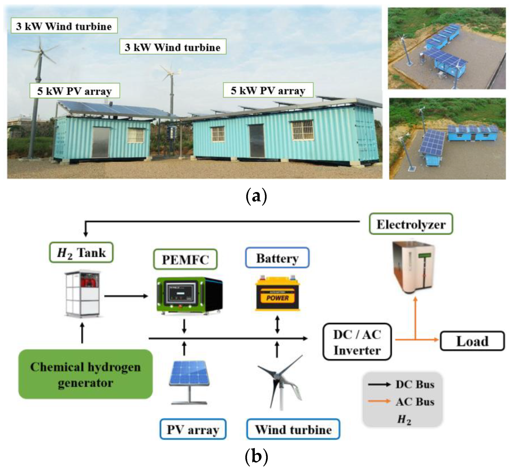
We consider a hybrid power system consisting of WTs, PVs, a PEMFC, batteries, chemical hydrogen production, and electrolyzers [23]. The system operates in a fully self-sufficient manner. Figure 1 illustrates the hybrid power system, in which wind and solar energy are the primary energy sources, while the fuel cell consumes hydrogen to provide backup power. Electrolyzers convert redundant energy to hydrogen, while chemical hydrogen production can generate hydrogen when necessary [14].
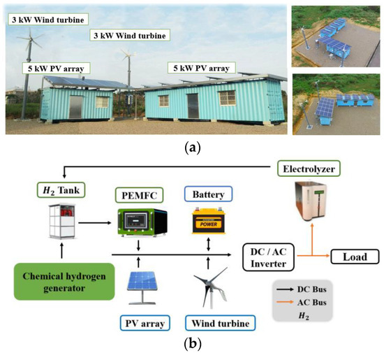
Figure 1.
The hybrid power system. (a) System construction. (b) System architecture.
The system was constructed in Miaoli County in Taiwan, where the initial components were selected based on the weather data from National Aeronautics and Space Administration to achieve seasonal complementarity between wind and solar energy. However, previous research has revealed that wind energy is insufficient to compensate for the deficit in solar energy during the winter. Additionally, a cost analysis indicated that wind power generation was more expensive than other energy forms [14]. Furthermore, the cost of using electrolyzers was higher than that of chemical hydrogen production [14]. Therefore, we conducted our extended-window designs for a hybrid power system consisting of PVs, batteries, a PEMFC, and chemical hydrogen production that could provide hydrogen by automatic batch processes [5].
We applied MATLAB Simscape ElectricalTM to develop the hybrid power model shown in Figure 2. The model enables us to estimate system responses under different operational conditions (e.g., varying components and PMS parameters) without extensive experimentation. The simulation model consisted of six modules: PVs, load, battery, PEMFC, chemical hydrogen generation, and power management with a prediction model [24].
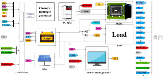
Figure 2.
Simulation model.
The PV module estimates the solar energy as follows [14,24]:
where is the solar current and is the DC-bus voltage. represents the solar radiation in units of W/m2. Solar energy is the primary energy source in this hybrid power system. The load module calculates the load current as follows:
where is the load power. The battery module regulates the energy storage and consumption of the system. We estimate the battery’s SOC by the following Coulomb integration method:
where is the battery SOC at time t, and C is the battery capacity. , , and represent the solar, PEMFC, and load currents, respectively, at time t. The PEMFC module acts as the system’s backup power and converts 1 L of hydrogen into 1.2620–1.2987 Wh of electricity. We applied a commercial 3 kW PEMFC, which provided reliable and consistent performance [25]. The hydrogen consumption rates are set as 12.32, 18.52, 24.64, and 30.75 standard L min−1, with PEMFC currents of 20 A, 30 A, 40 A, and 50 A, respectively [25]. The chemical hydrogen generation module provides hydrogen to the PEMFC when hydrogen is insufficient [5]. The sodium borohydride (NaBH4) solution is batched to generate 150 L of hydrogen each time, using 400 mL of 15wt% NaBH4 solution [14]. The power management module adjusts the PEMFC output current according to the battery SOC with the following PMS [14]:
- (a)
- When the battery SOC drops to , the prediction model is activated to forecast the solar radiation and load demand to calculate the battery SOC in the next 24 h.
- (b)
- If the battery SOC in the next 24 h is higher than 20%, the PEMFC remains silent and returns to Step (a). Otherwise, the PEMFC is activated to provide a supplementary power supply with the following current:where is the minimum SOC that happens at time T, supposing the present time is 0. represent the predicted solar and load currents, respectively, at time t. is the minimum PEMFC current to ensure the battery SOC was greater than 20%. The PEMFC current is set as when the required is estimated as and , respectively.
- (c)
- When the battery SOC reaches , the PEMFC is turned off and returns to Step (a). Otherwise, it returns to Step (b).
2.2. System Costs and Reliability
The system cost consists of the following two parts [24]:
where are the initial and operation costs, respectively. The subscripts b and s represent the sizes of the battery (in units of 100 Ah) and PV (in units of 1 kW), respectively.
The initial cost and operation cost are defined as follows [24]:
where k the represents system components, including PV, batteries, PEMFC, chemical hydrogen generation, and electronic devices. Conversely, m represents the components that require maintenance or incur operational costs, such as PVs and NaBH4.
The initial cost is estimated as follows [24]:
where represents the initial cost of module k per unit, is the units of module k, and CRF is the capital recovery factor [26]:
where ir represents the inflation rate (we set as ir = 1.26% in this paper) and ny represents the expected life of the module.
The operation cost of module m is estimated as follows [24]:
where is the unit operation or maintenance cost of module m, while is the required units or maintenance of m. For instance, the maintenance cost of the PV modules is set as 1% of its initial cost (i.e., ). Conversely, we set the unit operation cost for NaBH4 as , where is the unit cost for each batch that consumes 400 mL of 15wt% of NaBH4 solution, and is the number of batches. The component costs and lifespans are shown in Table 1. Finally, battery, PEMFC, and hydrogen costs depend on the system responses.

Table 1.
Prices and lives of system components.
Reliability is an important index when evaluating hybrid power systems, given the intermittent and unstable characteristics of renewable energy. We used the loss of power supply probability (LPSP) to indicate system reliability, defined as follows:
where is the required load demand and represents the loss of power supply at time t. The system reliability is highest when LPSP = 0%, indicating no power shortage.
2.3. Model Prediction for the Hybrid Power System
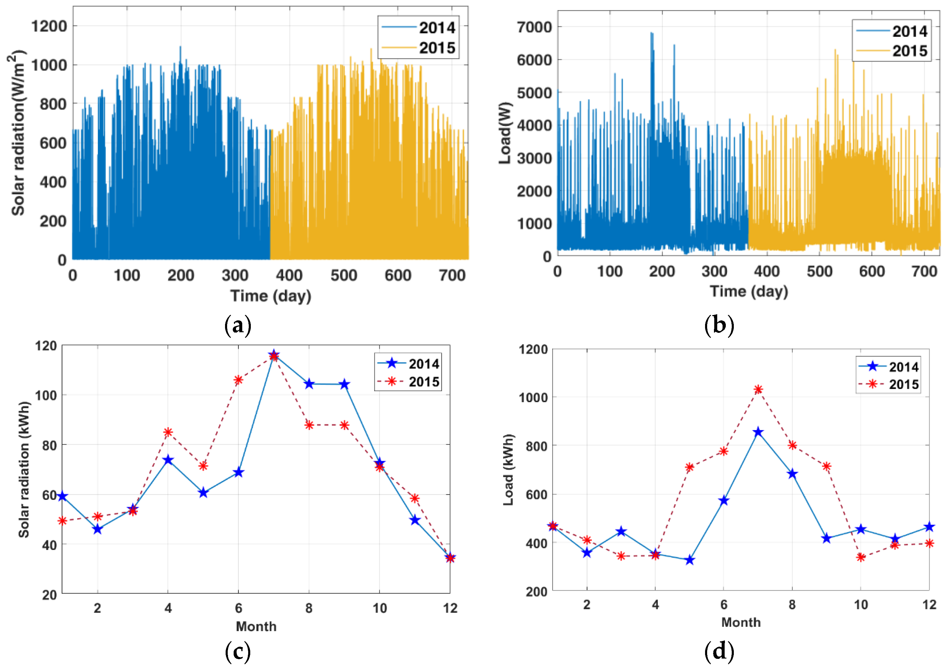
In previous research, we applied solar radiation [27] and load [28] data from 2014 to 2016 to optimize the design for a hybrid power system. Figure 3a illustrates the solar radiation data, showing a peak of 1094.44 W/m2 and 1083.33 W/m2, and an average daily availability of 2.31 kWh and 2.39 kWh in the first and second years, respectively. Figure 3b shows the load profiles, with peaks of 6.83 kW and 6.32 kW, and average daily consumptions of 15.91 kWh and 18.41 kWh in the first and second years, respectively.
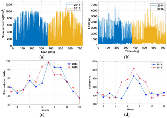
Figure 3.
Solar and load data in two years. (a) Solar responses. (b) Load profiles. (c) Average monthly solar responses. (d) Average monthly load profiles.
We applied the Simscape model with these solar and load data to optimize the system designs. The results are illustrated in Table 2. First, Case-a used the 2014 data to optimize system settings, resulting in (b, s) = (13, 11) and (SOClow, SOChigh) = (40%, 50%). We then applied these optimal settings to estimate system responses in 2015 without model prediction, where the system cost is USD 0.7889/kWh and the hydrogen consumption is 468,007.2 L, for a system reliability of LPSP = 0%. Second, Case-A applied the same optimal setting to estimate system responses in 2015 with XGBoost prediction models [14]. The system cost was reduced to USD 0.7389/kWh, and the hydrogen consumption decreased to 311,683.9 L, while maintaining system reliability LPSP = 0%. The results showed that model prediction can significantly reduce system costs and hydrogen consumption by 6.45% and 33.40%, respectively.
Table 2.
Comparison of system optimization with/without model predictions.
2.4. Extended-Window Algorithms for Model Prediction
Table 2 shows that model prediction can reduce system costs while maintaining system sustainability. However, our previous optimization [14] applied annual data to optimize system components and PMS only once for the entire second year. Figure 3c,d shows that the solar and load data varied significantly during the year. This raised the possibility that system performance might be further improved by updating the optimal system settings more frequently. Therefore, we proposed the extended-window algorithms for model prediction.
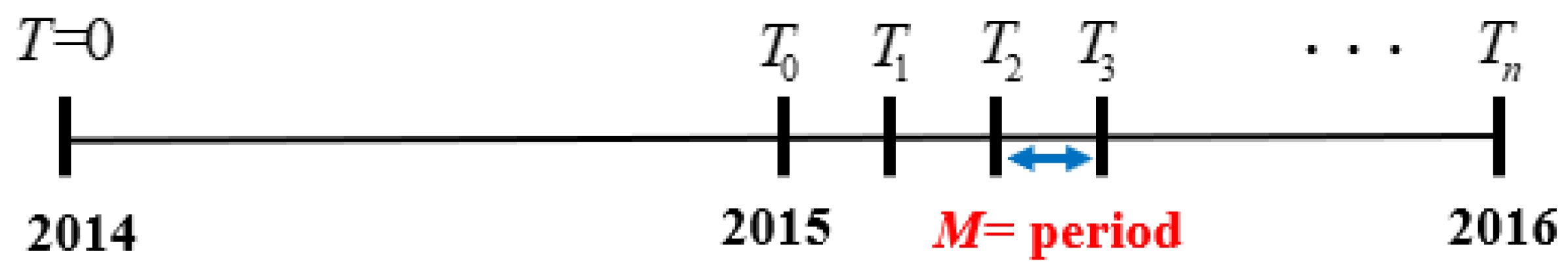
The principle of the extended-window algorithms is to train the prediction models periodically using the accumulated data, as shown in Figure 4, to enable the system to re-estimate the optimal components and PMS at each interval. Suppose the interval length is M, which might be one month, one week, and so on. We set , and the remaining time . The procedures are as follows:

Figure 4.
Extended-window model prediction.
- (a)
- Set i = 1.
- (b)
- Use the radiation and load data in to train the prediction models.
- (c)
- Apply the prediction models obtained in step (b) to forecast the solar current and load responses in the next interval , labeled as for .
- (d)
- Use to optimize system components and PMS for the interval , denoted as and .
- (e)
- Apply the optimal settings in step (d) to the interval . Calculate the system costs and hydrogen consumption in this interval.
- (f)
- Complete the design when i = n. Otherwise, increase i by one and return to step (b).
The extended-window model prediction derives optimal system components and PMS at each interval while updating system components periodically. Therefore, we add the component replacement costs and adjust the system cost as follows:
where represents the replacement costs, defined as follows:
where p is the adjusted components, including the PV and batteries. represents the replacement cost of component p, while is the replaced units of the component p. The unit replacement cost is , where is the replacement cost ratio and is the initial unit cost of component p.
3. Results
This section applies the extended-window model prediction to the hybrid power system. We developed five prediction models and chose the two best models to foretell the solar and load responses. We then applied these models to investigate the merits of the proposed extended-window method for optimizing the hybrid power system.
3.1. Optimal Prediction Models
Many artificial intelligent algorithms have been applied to hybrid power systems, such as XGBoost, LightGBM, CatBoost, K-Nearest Neighbors (KNN), and Random Forest (RF). The details of these algorithms are illustrated in Appendix A. We applied these algorithms to build the prediction models and evaluated their performance by the normalized root mean square error (NRMSE), defined as follows:
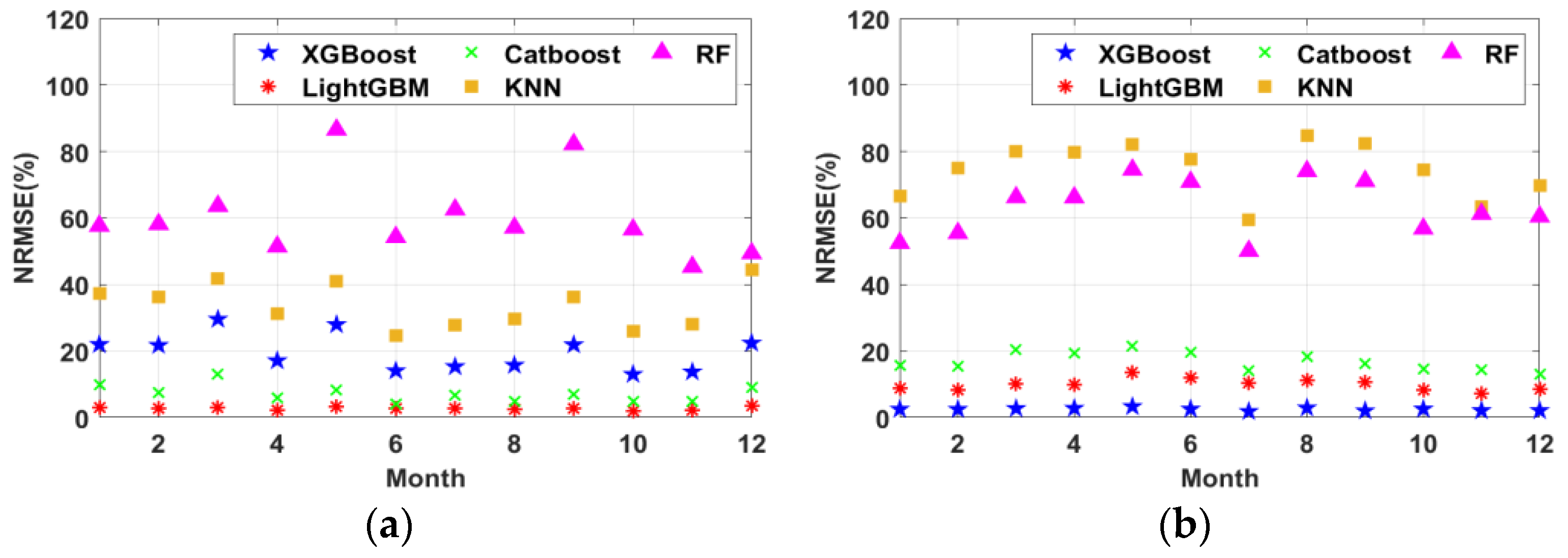
where and were the real and predictive data, respectively, at the i-th sample, N represented the number of samples, and was the average of real data y. Figure 5 and Table 3 illustrate the NRMSEs of different prediction models using the extended-window method with M = 1 month and . The LightGBM and XGBoost models can successfully forecast solar radiation and load demand with an accuracy of 97.25% and 97.49%, respectively. Hence, we apply these two models to analyze the system performance.
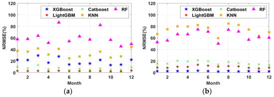
Figure 5.
Performance comparison of five prediction models. (a) Solar radiation. (b) Load profiles.
Table 3.
NRMSE of extended-window prediction models with M = 1 month.
As shown in Table 3, the LightGBM and XGBoost models can predict solar radiation and load profiles with minor prediction errors. We further investigate the impacts of these small prediction errors on system performance by comparing them with the system employing perfect predictions. The perfect prediction is defined as using the real data instead of the predicted for when optimizing the components and PMS in each interval. For example, we set the interval length M = 1 month and the replacement cost ratio . When using the perfect prediction, the annual system cost was USD 4607.95, with a hydrogen consumption of 102,343.9 L. When using the prediction models, the annual system cost became USD 4599.35, with a hydrogen consumption of 108,248.70 L. These results show that the influences of these minor prediction errors are negligible
3.2. Impacts of Window Sizes and Replacement Costs
We analyzed the influences of interval length M and replacement cost ratio on system cost and hydrogen consumption. We compared the results with Case A in three scenarios: varied M, different , and simultaneously varied M and .
First, we set to investigate the impact of interval length M on system performance. The results are shown in Table 4, where M = [6, 4, 3, 2, 1] months, [3, 2, 1] weeks, and 5 days. The system reliability LPSP = 0% in all cases, while the system costs and hydrogen consumption gradually decline as M decreases until M = 1 week. The optimal extended-window designs when M = 1 week are illustrated in Appendix B. Compared with Case A, the optimal cost reduction is 13.57% and the optimal hydrogen savings is 91.64% when M = 1 week. Setting M = 5 days worsened the system cost and hydrogen consumption, possibly because M = 5 days is not a suitable periodicity for data segmentation.
Table 4.
Impacts of interval length ().
Second, we set M = 1 month to investigate the impacts of replacement cost ratio. The results are shown in Table 5, where the system reliability LPSP = 0% in all cases. When the replacement cost increases, the system makes fewer component adjustments between consecutive intervals to avoid unnecessary replacement costs. Compared with Case A, when , the cost and hydrogen reduction were 7.24% and 65.27%, respectively. When , the cost and hydrogen reduction were 1.86% and 53.18%, respectively.
Table 5.
Impacts of replacement cost ratio (M = 1 month).
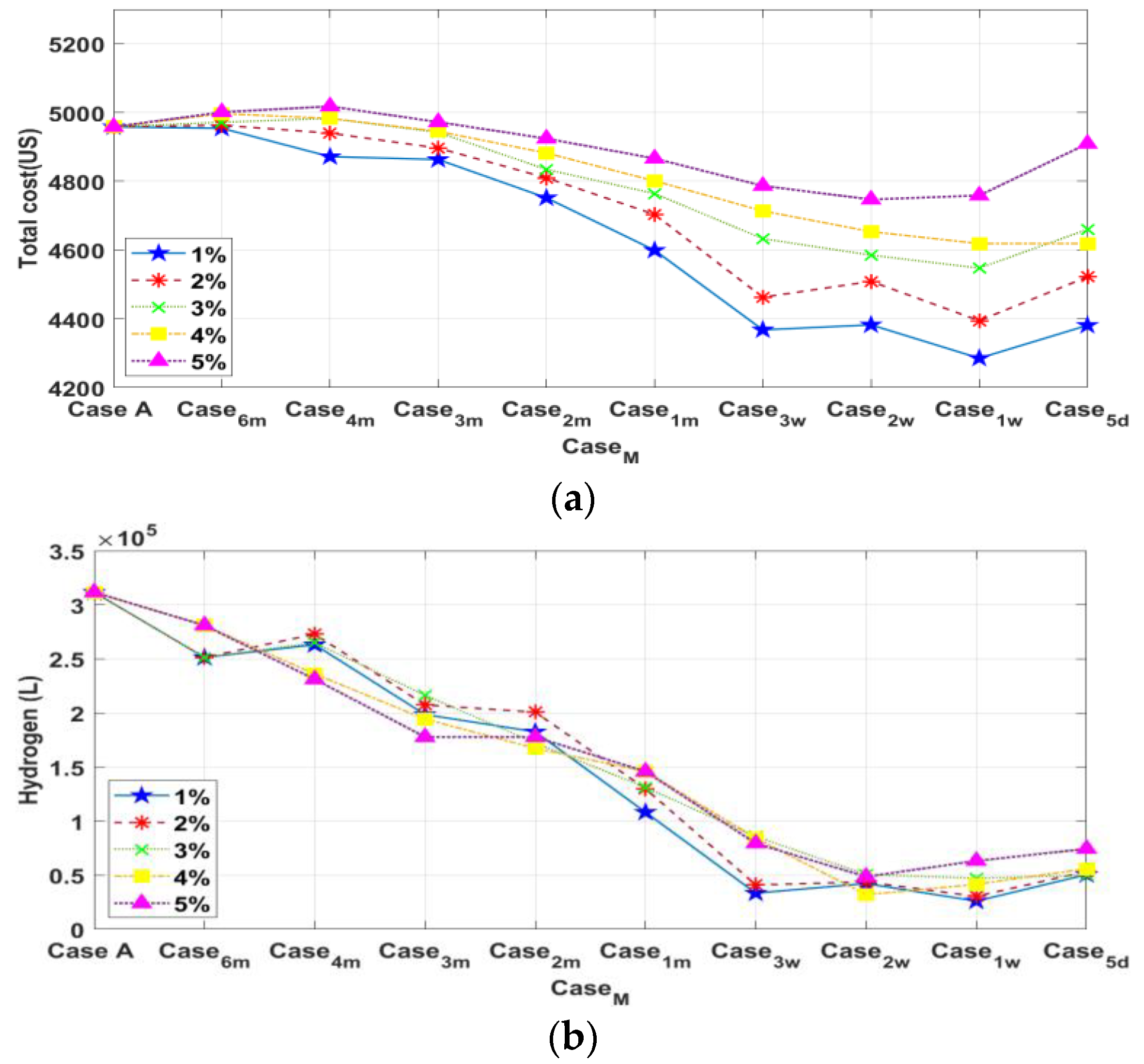
Finally, we discuss the integrated impacts of the interval length M and the replacement cost ratio . The results are shown in Figure 6, where the system reliability LPSP = 0% in all cases. As shown in Figure 6, M = 1 week is the optimal interval for system costs and hydrogen consumption regardless of . The hydrogen reduction is over 70% for . Furthermore, Figure 6a illustrates the limits on cost reduction, where M = 1 week is the optimal interval length. Setting a shorter M = 5 days leads to an increase in system costs, possibly because this interval is unsuitable for data segmentation. Hence, the periodicity of data segmentation and the replacement expenses should be considered when optimizing system designs using the extended-window model prediction.
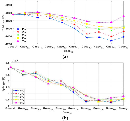
Figure 6.
Combined effects of interval length M and replacement cost ratio . (a) System costs. (b) Hydrogen consumption.
4. Discussion
This paper proposes extended-window algorithms for model prediction. We then applied them to a hybrid power system consisting of a PV, batteries, PEMFC, and chemical hydrogen production system. The proposed method enables the periodic adjustment of the system components and PMS based on accumulated data.
We applied MATLAB Simscape ElectricalTM to develop a hybrid power model that enables the estimation of system responses without extensive experimentation. We then applied five machine learning methods to develop prediction models for our hybrid power system. The results showed that the LightGBM and XGBoost models could forecast solar radiation and load profiles with a higher than 97% accuracy. Therefore, we integrated these two models into the hybrid power system to investigate the impacts of extended-window model prediction on system performance.
First, we assessed the impact of interval length M on system performance. The results showed that system cost and hydrogen consumption gradually decreased when we shortened the window size M to M = 1 week. Therefore, the regular modification of system components and power management could improve system performance. However, there was a limit. For example, setting M = 5 days slightly increased the system costs.
Second, we investigated the influences of replacement costs. The results showed that the system made fewer component adjustments when the replacement cost increased to avoid replacement expenses. Hence, increasing the replacement cost could eliminate the cost reduction afforded by the proposed extended-window model prediction. For instance, the cost reduction was 7.24% when and was 1.86% when .
Finally, we examined the integrated effects of interval length M and replacement cost ratio . The results indicated that M = 1 week is the optimal interval for reducing system costs and hydrogen consumption regardless of . Conversely, increasing the replacement cost ratio tended to demolish the merits of the extended-window method because the system tended to make fewer component changes.
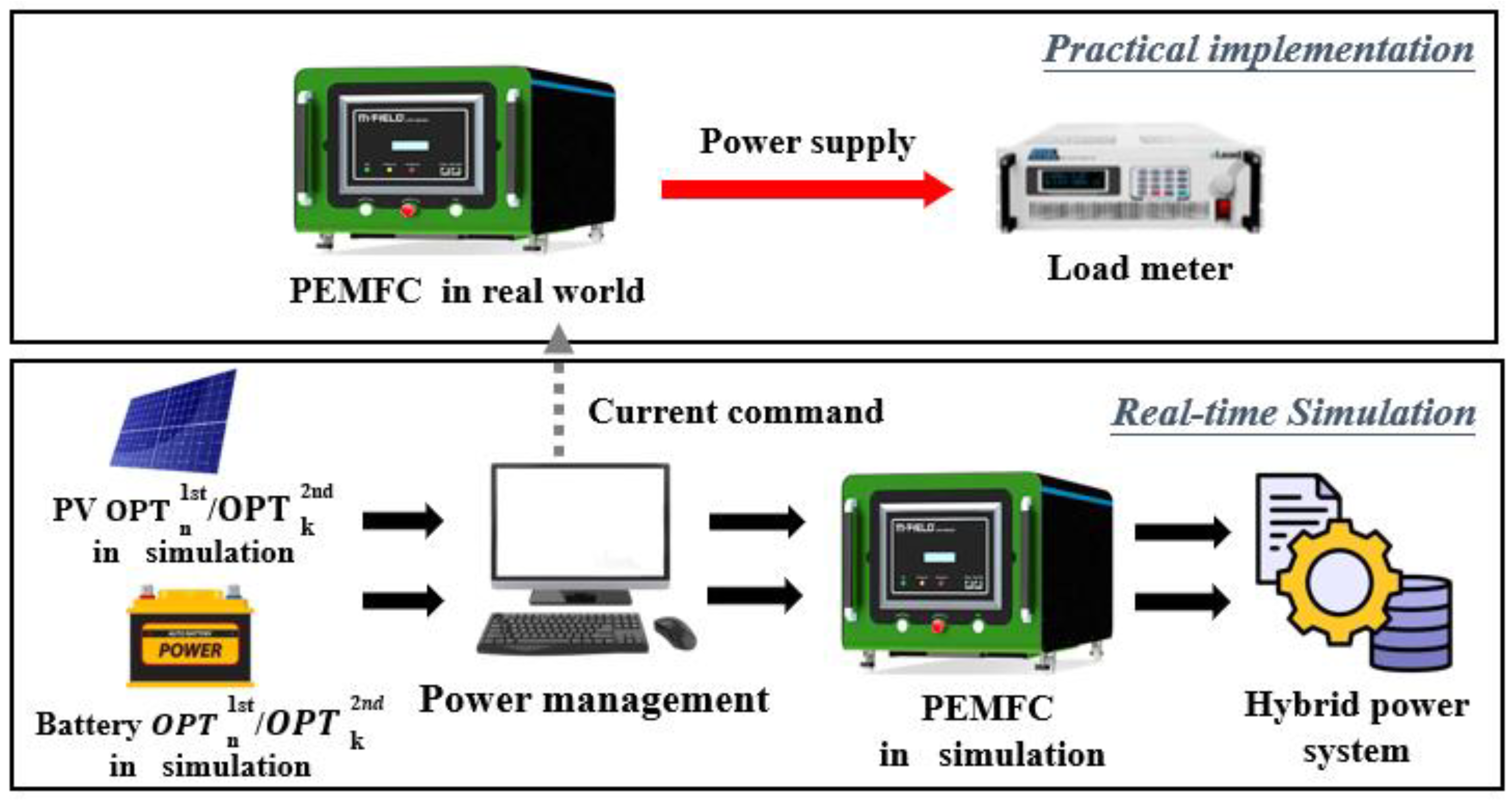
To demonstrate the proposed method’s effectiveness and feasibility, we designed experiments using a hybrid power system that employs the extended-window optimization. The experiment configuration is shown in Figure 7 and consists of real-time simulation and physical implementation.

Figure 7.
The experimental settings.
The real-time simulation applied the optimal system settings of two periods when M = 5 days and : Period I is 16–20 April 2015 and Period II is 21–25 April 2015. In Period I, the optimal settings are (b, s) = (8, 5) and (SOClow, SOChigh) = (40%, 50%). With no extended-window model prediction, the optimal settings remained the same in Period II. With extended-window model prediction, the optimal settings became (b, s) = (10, 7) and (SOClow, SOChigh) = (40%, 50%) in period II. The practical implementation consists of a PEMFC and a loadmeter. When the system needed supplementary power, the simulation model sent current commands to the PEMFC, which was then physically activated to provide the required current. The original period was ten days; we applied a scale factor of 1/600 to shorten the experimental time to 24 min, with the initial SOC = 30%. We measured system signals, such as the currents and voltages, to detect signs of potentially declining efficiency.
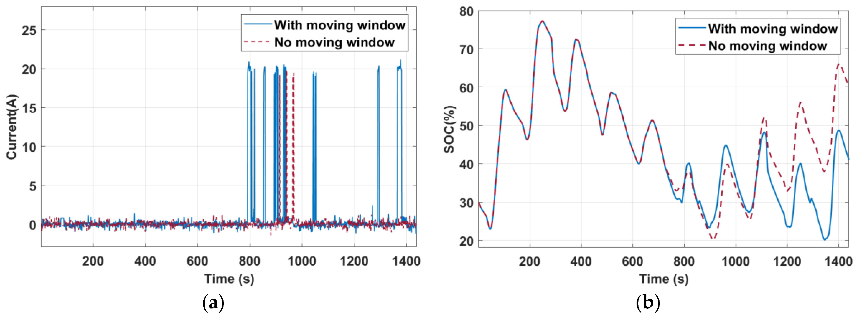
The system responses are shown in Figure 8 and Table 6. Because the initial SOC was 30%, the system immediately predicted the system SOC for the following 24 h until t = 87 s, when the system SOC exceeded a threshold SOC = 50%. At Period I, the predicted SOC for the next 24 h remained above 20%, indicating a sufficient power supply without the PEMFC. The system cost was USD 37.66 and the hydrogen consumption was zero. At t = 720 s, the system reached the second interval; the original system settings (b, s) = (8, 5) gave a system cost of USD 81.06 and a hydrogen consumption of 17,740.8 L. Using the extended-window model prediction, the optimal system settings were updated as (b, s) = (10, 7), and the system cost became USD 54.04, with a hydrogen consumption of 3942.4 L. The extended-window optimization reduced the system costs and hydrogen consumption by 22.76% and 77.78%, respectively. Finally, the system was sustainable because the system SOC was maintained above 20% in both cases, as shown in Figure 8b.
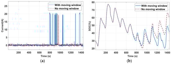
Figure 8.
Experimental responses. (a) PEMFC current. (b) Battery SOC.
Table 6.
Statistical data of Figure 8.
We also designed an energy module, as shown in Figure 9a, to demonstrate the feasibility of adjusting system components in real time. The module consisted of a 48 V 22 Ah battery, a foldable 180 W PV panel, and a maximum power point tracking controller between the PV panels and the DC bus to maximize the output solar power. We used the ANCHI connector as a hot-wired component, as shown in Figure 9b. The subsequent experiments showed that the module could share the load demands by hot plugging in real time. Suppose the load demand was 5 A; the system responses are shown in Figure 9c,d. First, the primary battery provided the load of 5 A alone, so its SOC decreased at −0.0062%/s. At t = 1200 s, its SOC dropped to 46.24%, and the energy module was hot plugging into the primary system through the ANCHI connector to provide the loads and raise the primary battery SOC at a rate of 0.0016%/s. Because the experiments were conducted indoors, we simulated the PV panel by applying a power supply, which provided a constant solar current . Finally, the energy module was disconnected from the primary system in real time by hot swapping at t = 2400 s. The primary system’s battery again provided a load of 5 A, with a decreasing rate of −0.0062%/s for the SOC. These results confirm the feasibility of operating a power system with periodic adjustments of the components.
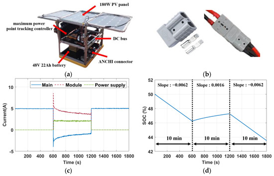
Figure 9.
The energy module and experiments. (a) Module architecture. (b) ANCHI connector [29]. (c) Current responses. (d) Main battery SOC.
5. Conclusions
This paper proposed the use of extended-window algorithms for model prediction with applications in hybrid power systems. We considered a PV, batteries, PEMFC, and chemical hydrogen production system. The proposed methods could periodically adjust system components and PMS based on solar energy and load predictions. We developed a hybrid power model to estimate system responses at different operational conditions. We then built five machine learning models and selected the LightGBM and XGBoost models to forecast solar radiation and load.
We applied a two-year dataset to investigate the merits of extended-window model prediction. Regarding the window size, the results showed that shortening the interval could reduce system costs, with an optimal interval of one week. Regarding the replacement costs, the system tended to make fewer replacements to decrease expenses when the replacement costs were higher. Combining these analyses, we concluded that weekly system updates yielded the lowest costs. The optimal cost and hydrogen reduction were 13.57% and 91.64%, respectively, compared to the system that did not employ the extended-window algorithms.
Finally, we designed experiments to demonstrate the feasibility of a hybrid power system employing extended-window model prediction. The experimental results showed that the extended-window optimization significantly reduced the system costs and hydrogen consumption by 22.76% and 77.78%, respectively. We also designed a renewable energy module that could hot plug into the system DC bus in real time to illustrate the feasibility of using hybrid power systems that adopt the proposed method.
In this paper, the system parameters were selected according to system loads. For example, in the first year, the maximum load and average daily power consumption were 6.83 kW and 15.91 kWh, respectively. Therefore, we applied a 3 kW PEMFC to guarantee system sustainability, and we set the PV modules in units of 1 kW and the battery modules in units of 48 V–100 Ah. These settings must be adjusted if the system’s power level changes [30]. In addition, other components, such as supercapacitors [30], might also be integrated with the hybrid power systems. Finally, we have not considered battery degradation to simplify system designs. When considering battery degradation, the battery needs to be replaced more frequently to maintain system sustainability so that the system costs will be increased. However, periodic adjustments of the prediction models based on accumulated data are potentially beneficial in reducing system costs because they can at least retain the same system settings and prediction models as those without employing the extended-window algorithms. The proposed extended-window algorithms can be applied to systems with different layouts and settings for performance improvement.
Author Contributions
Conceptualization, F.-C.W.; methodology, F.-C.W.; software, H.-T.H.; validation, F.-C.W. and H.-T.H.; formal analysis, F.-C.W. and H.-T.H.; investigation, F.-C.W. and H.-T.H.; resources, F.-C.W.; data curation, H.-T.H.; writing—original draft preparation, F.-C.W. and H.-T.H.; writing—review and editing, F.-C.W. and H.-T.H.; visualization, F.-C.W. and H.-T.H.; supervision, F.-C.W.; project administration, F.-C.W.; funding acquisition, F.-C.W. All authors have read and agreed to the published version of the manuscript.
Funding
This research was funded by the Ministry of Science and Technology, Taiwan under MOST 106-2221-E-002-165-, MOST 107-2221-E-002-174-, MOST 108-2221-E-002-086-, and MOST 109-2622-E-002-011-CC3.
Institutional Review Board Statement
Not applicable.
Informed Consent Statement
Not applicable.
Data Availability Statement
The weather and load data are available at http://140.112.14.7/~sic/PaperMaterial/Prediction_weather_load_data.csv (accessed on 19 November 2023).
Acknowledgments
The authors thank M-FieldTM for their collaboration and technical support.
Conflicts of Interest
The authors declare no conflicts of interest.
Appendix A
The five machine learning algorithms are briefly introduced as follows:
- (1)
- eXtreme Gradient Boosting (XGBoost)
The XGBoost algorithm is a machine learning method known for its rapid training speed and high accuracy. It is designed to transform multiple base learners into strong learners, constructing a sequence of interconnected trees. Each base learner functioned as a classification or regression tree, and every tree is linked to its predecessor. By adjusting weights, XGBoost corrects errors and enhances predictive precision. This algorithm operates by classifying data points at various nodes in the tree structure.
Given that a single tree might struggle to make accurate predictions, XGBoost combines multiple trees and creates an ensemble of trees that collectively contribute to the model. Each tree is assigned the task of discerning distinct features. The computational methodology is as follows [31]:
where is the feature i, signifies the predicted outcome of feature i, and denotes the predictive score of feature i in the k-th tree. Subsequently, we optimized the structure of the trees using the following objective loss function:
where is the loss function, which calculates the disparity between the actual value and predicted value , and is a regularization term that both smooths the final learning weights and controls the complexity of the model to prevent overfitting.
- (2)
- Light Gradient Boosting Machine (LightGBM)
LightGBM is a free and open-source machine learning framework developed by Microsoft in 2016, designed for tackling classification and regression problems. It is built upon the foundation of a traditional Gradient Boosting Machine (GBM) while introducing optimizations and enhancements. One of its key innovations was utilizing a Gradient-Based One-Side Sampling (GOSS) technique, which aimed to maintain accuracy while effectively handling large datasets. Additionally, LightGBM employs Exclusive Feature Bundling (EFB) to reduce the feature count by bundling mutually exclusive features. This innovative approach helps enhance performance and efficiency in various machine learning tasks [32].
- (3)
- CatBoost
CatBoost is a framework based on gradient-boosting decision tree models. The algorithm’s name originates from the words “Category” and “Boost”, highlighting its focus on categorical features within the dataset. Since categorical features consist of a discrete set of categories, the typical technique for handling them in boosting methods is one-hot encoding, which adds a binary feature for each category present in the original feature. However, for high cardinality features, this approach can lead to an explosion in the number of features. CatBoost also introduces a sorting algorithm that leverages ordered target statistics, which evolves from mean encoding. This technique addresses prediction shift problems arising from distribution differences between training and testing datasets. It handles categorical features with fewer categories using one-hot encoding. For other categorical features, CatBoost employs an efficient encoding approach similar to mean encoding but with an additional mechanism to reduce overfitting [33].
- (4)
- K-Nearest Neighbors (KNN)
KNN is one of the simplest machine learning algorithms for classification and regression analyses. It falls under supervised learning algorithms and employs “feature similarity” to predict values for new data points. KNN assigns a value to the new point based on its resemblance to nearby points by assessing the similarity between a new data point and points within the training set. In the context of regression problems, predicting the value of a point involves calculating the average of the values of its K nearest neighbors. There are three ways to calculate the distance: the Euclidean distance, which refers to the actual distance between two points in N-dimensional space; the Manhattan distance, which indicates the absolute wheelbase sum of the two points in the coordinate system; and the Minkowski distance, which generalizes both the Euclidean and Manhattan distances [34].
- (5)
- Random Forest (RF)
RF belongs to supervised learning, encompassing accuracy, simplicity, and flexibility. It stands as one of the most commonly employed algorithms. Its fundamental principle revolves around the amalgamation of multiple Classification and Regression Trees (CART) alongside the inclusion of randomly distributed training data. This incorporation significantly enhances the ultimate predictive outcomes. RF is capable of integrating multiple base learners to construct a potent learner. This approach is also referred to as Ensemble Learning. Within this context, RF uses Bagging in Ensemble Learning, which involves resampling the original dataset to generate new ones. The resampling process is uniform and allows for repetition, enabling the creation of multiple sets of new datasets through bootstrapping. From these datasets, K samples are extracted and used to train K learners. Each time, the K samples are drawn with replacements from the original dataset, which means that some data might be duplicated across these K samples. However, the trained learners exhibited diversity due to the inherent variability resulting from the slight differences in the composition of training samples for each learner. The outcome was obtained through majority voting (classification) or averaging (regression) [35].
Appendix B
The optimal system settings employing the extended-window design with M = 1 week and r% = 1% are illustrated in Table A1.
Table A1.
The optimal settings with M = 1 week and r% = 1%.
Table A1.
The optimal settings with M = 1 week and r% = 1%.
| Period | (b, s) | (SOClow, SOChigh) | System Cost (USD) | Hydrogen Consumption (L) |
|---|---|---|---|---|
| 1st | (14, 9) | (25%, 30%) | 74.17 | 0 |
| 2nd | (14, 12) | (30%, 35%) | 88.31 | 862.4 |
| 3rd | (18, 9) | (25%, 30%) | 80.78 | 0 |
| 4th | (11, 9) | (25%, 30%) | 71.87 | 0 |
| 5th | (13, 12) | (25%, 30%) | 88.79 | 1479.2 |
| 6th | (16, 23) | (40%, 45%) | 191.2 | 21,628.4 |
| 7th | (7, 5) | (25%, 30%) | 59.49 | 0 |
| 8th | (8, 9) | (25%, 30%) | 68.4 | 0 |
| 9th | (11, 8) | (25%, 30%) | 68.41 | 0 |
| 10th | (11, 14) | (40%, 45%) | 92.55 | 0 |
| 11th | (11, 5) | (30%, 35%) | 59.83 | 123.2 |
| 12th | (13, 8) | (25%, 30%) | 71.4 | 0 |
| 13th | (20, 6) | (30%, 35%) | 72.48 | 123.2 |
| 14th | (12, 3) | (25%, 30%) | 51.77 | 0 |
| 15th | (26, 6) | (35%, 40%) | 81.88 | 369.6 |
| 16th | (7, 6) | (25%, 30%) | 57.59 | 0 |
| 17th | (7, 5) | (35%, 40%) | 52.6 | 0 |
| 18th | (13, 6) | (25%, 30%) | 63.12 | 0 |
| 19th | (30, 16) | (25%, 30%) | 127.7 | 0 |
| 20th | (14, 6) | (25%, 30%) | 69.17 | 0 |
| 21th | (17, 26) | (25%, 30%) | 149.5 | 0 |
| 22th | (17, 9) | (35%, 40%) | 84.15 | 0 |
| 23th | (12, 7) | (45%, 50%) | 68.36 | 0 |
| 24th | (20, 8) | (25%, 30%) | 80.25 | 0 |
| 25th | (19, 11) | (25%, 30%) | 89.74 | 0 |
| 26th | (16, 8) | (35%, 40%) | 76.25 | 0 |
| 27th | (16, 8) | (45%, 50%) | 75.1 | 0 |
| 28th | (26, 11) | (25%, 30%) | 99.8 | 0 |
| 29th | (28, 12) | (25%, 30%) | 103.2 | 0 |
| 30th | (16, 9) | (25%, 30%) | 79.67 | 0 |
| 31th | (19, 9) | (45%, 50%) | 81.55 | 0 |
| 32th | (21, 8) | (25%, 30%) | 80.48 | 0 |
| 33th | (17, 12) | (25%, 30%) | 91.15 | 0 |
| 34th | (18, 9) | (25%, 30%) | 80.29 | 0 |
| 35th | (27, 24) | (40%, 45%) | 152.7 | 0 |
| 36th | (18, 11) | (25%, 30%) | 93.36 | 0 |
| 37th | (17, 8) | (45%, 50%) | 76.76 | 0 |
| 38th | (16, 6) | (25%, 30%) | 66.32 | 0 |
| 39th | (19, 11) | (25%, 30%) | 90.78 | 0 |
| 40th | (10, 4) | (25%, 30%) | 56.18 | 0 |
| 41th | (13, 6) | (25%, 30%) | 62.98 | 0 |
| 42th | (10, 5) | (25%, 30%) | 56.02 | 0 |
| 43th | (11, 6) | (25%, 30%) | 61.49 | 0 |
| 44th | (12, 11) | (25%, 30%) | 81.88 | 0 |
| 45th | (6, 5) | (25%, 30%) | 53.99 | 0 |
| 46th | (12, 6) | (25%, 30%) | 61.9 | 0 |
| 47th | (12, 9) | (40%, 45%) | 73.36 | 739.2 |
| 48th | (11, 8) | (25%, 30%) | 68.08 | 0 |
| 49th | (12, 14) | (25%, 30%) | 95.05 | 0 |
| 50th | (11, 9) | (25%, 30%) | 72.43 | 0 |
| 51th | (14, 11) | (25%, 30%) | 83.61 | 0 |
| 52th | (12, 23) | (25%, 30%) | 147.8 | 0 |
References
- The Net Zero Strategy in UK. Available online: https://www.re.org.tw/knowledge/more.aspx?cid=201&id=5439 (accessed on 5 August 2023).
- Japan Eyes Over 108 GW Solar Power Capacity by 2030. Available online: https://taiyangnews.info/markets/japan-eyes-over-108-gw-solar-power-capacity-by-2030/ (accessed on 16 August 2023).
- Powering a Climate-Neutral Economy: Commission Sets out Plans for the Energy System of the Future and Clean Hydrogen. Available online: https://ec.europa.eu/commission/presscorner/detail/en/ip_20_1259 (accessed on 5 August 2023).
- International Trends of Energy. Available online: https://www.trademag.org.tw/page/itemsd/?id=7873730&no=21 (accessed on 5 August 2023).
- Li, S.-C.; Wang, F.-C. The development of a sodium borohydride hydrogen generation system for proton exchange membrane fuel cell. Int. J. Hydrogen Energy 2016, 41, 3038–3051. [Google Scholar] [CrossRef]
- Taghizadeh, M.; Mardaneh, M.; Sadeghi, M.S. Frequency control of a new topology in proton exchange membrane fuel cell/wind turbine/photovoltaic/ultra-capacitor/battery energy storage system based isolated networks by a novel intelligent controller. J. Renew. Sustain. Energy 2014, 6, 053121. [Google Scholar] [CrossRef]
- Bornapour, M. Optimal stochastic scheduling of CHP-PEMFC, WT, PV units and hydrogen storage in reconfigurable micro grids considering reliability enhancement. Energy Convers. Manag. 2017, 150, 725–741. [Google Scholar] [CrossRef]
- Shayan, M.E.; Ghasemzadeh, F.; Rouhani, S.H. Energy storage concentrates on solar air heaters with artificial S-shaped irregularity on the absorber plate. J. Energy Storage 2023, 74, 109289. [Google Scholar] [CrossRef]
- Zhao, K. Analysis of a hybrid system combining solar-assisted methanol reforming and fuel cell power generation. Energy Convers. Manag. 2023, 297, 117664. [Google Scholar] [CrossRef]
- Rouhani, A.; Kord, H.; Mehrabi, M. A comprehensive method for optimum sizing of hybrid energy systems using intelligence evolutionary algorithms. Indian J. Sci. Technol. 2013, 6, 4702–4712. [Google Scholar] [CrossRef]
- N’guessan, S.A. Optimal sizing of a wind, fuel cell, electrolyzer, battery and supercapacitor system for off-grid applications. Int. J. Hydrogen Energy 2020, 45, 5512–5525. [Google Scholar] [CrossRef]
- Lei, G.; Song, H.; Rodriguez, D. Power generation cost minimization of the grid-connected hybrid renewable energy system through optimal sizing using the modified seagull optimization technique. Energy Rep. 2020, 6, 3365–3376. [Google Scholar] [CrossRef]
- Šimunović, J.; Radica, G.; Barbir, F. The effect of components capacity loss on the performance of a hybrid PV/wind/battery/hydrogen stand-alone energy system. Energy Convers. Manag. 2023, 291, 117314. [Google Scholar] [CrossRef]
- Wang, F.-C.; Wang, J.-Z. Superior Optimization for a Hybrid PEMFC Power System Employing Model Predictions. Int. J. Energy Res. 2023, 2023, 9984961. [Google Scholar] [CrossRef]
- Park, J. Multistep-ahead solar radiation forecasting scheme based on the light gradient boosting machine: A case study of Jeju Island. Remote Sens. 2020, 12, 2271. [Google Scholar] [CrossRef]
- Vu, D.H.; Muttaqi, K.M.; Agalgaonkar, A.P. Short-term load forecasting using regression based moving windows with adjustable window-sizes. In Proceedings of the 2014 IEEE Industry Application Society Annual Meeting, Vancouver, BC, Canada, 5–9 October 2014. [Google Scholar]
- Bae, D.-J.; Kwon, B.-S.; Song, K.-B. XGBoost-based day-ahead load forecasting algorithm considering behind-the-meter solar PV generation. Energies 2021, 15, 128. [Google Scholar] [CrossRef]
- Brka, A.; Kothapalli, G.; Al-Abdeli, Y.M. Predictive power management strategies for stand-alone hydrogen systems: Lab-scale validation. Int. J. Hydrogen Energy 2015, 40, 9907–9916. [Google Scholar] [CrossRef]
- Brka, A.; YAl-Abdeli, M.; Kothapalli, G. Predictive power management strategies for stand-alone hydrogen systems: Operational impact. Int. J. Hydrogen Energy 2016, 41, 6685–6698. [Google Scholar] [CrossRef]
- Nair, U.R.; Costa-Castelló, R. A model predictive control-based energy management scheme for hybrid storage system in islanded microgrids. IEEE Access 2020, 8, 97809–97822. [Google Scholar] [CrossRef]
- Kodakkal, A. An optimized enhanced phase locked loop controller for a hybrid system. Technologies 2022, 10, 40. [Google Scholar] [CrossRef]
- Shayan, M.E. A novel approach of synchronization of the sustainable grid with an intelligent local hybrid renewable energy control. Int. J. Energy Environ. Eng. 2023, 14, 35–46. [Google Scholar] [CrossRef]
- Green Building Project Introduction. Available online: https://www.ceci.org.tw/modules/article-content.aspx?s=33&i=372 (accessed on 2 August 2023).
- Chen, P.-J.; Wang, F.-C. Design optimization for the hybrid power system of a green building. Int. J. Hydrogen Energy 2018, 43, 2381–2393. [Google Scholar] [CrossRef]
- Guo, Y.-F.; Chen, H.-C.; Wang, F.-C. The development of a hybrid PEMFC power system. Int. J. Hydrogen Energy 2015, 40, 4630–4640. [Google Scholar] [CrossRef]
- Annual Growth Rate of CPI. Available online: https://data.oecd.org/price/inflation-cpi.htm (accessed on 2 August 2023).
- CWB Observation Data Inquire System. Available online: https://codis.cwa.gov.tw/ (accessed on 2 August 2023).
- Wang, F.-C. Fuel-cell sharing for a distributed hybrid power system. Int. J. Hydrogen Energy 2021, 46, 1174–1187. [Google Scholar] [CrossRef]
- ANKG Company Data. Available online: https://www.zhaosw.com/product/detail/258992780 (accessed on 2 August 2023).
- Liu, X. Sponge Supercapacitor rule-based energy management strategy for wireless sensor nodes optimized by using dynamic programing algorithm. Energy 2022, 239, 122368. [Google Scholar] [CrossRef]
- Chen, T.; Guestrin, C. Xgboost: A scalable tree boosting system. In Proceedings of the 22nd ACM SIGKDD International Conference on Knowledge Discovery and Data Mining, San Francisco, CA, USA, 13 August 2016. [Google Scholar]
- Fan, J. Light Gradient Boosting Machine: An efficient soft computing model for estimating daily reference evapotranspiration with local and external meteorological data. Agric. Water Manag. 2019, 225, 105758. [Google Scholar] [CrossRef]
- Prokhorenkova, L. CatBoost: Unbiased boosting with categorical features. Adv. Neural Inf. Process. Syst. 2018, 31. [Google Scholar] [CrossRef]
- Guo, G. KNN model-based approach in classification. In Proceedings of the CoopIS, DOA, and ODBASE 2003 Catania, Sicily, Italy, 3–7 November 2003. [Google Scholar]
- Jordan, M.I.; Mitchell, T.M. Machine learning: Trends, perspectives, and prospects. Science 2015, 349, 255–260. [Google Scholar] [CrossRef]


Disclaimer/Publisher’s Note: The statements, opinions and data contained in all publications are solely those of the individual author(s) and contributor(s) and not of MDPI and/or the editor(s). MDPI and/or the editor(s) disclaim responsibility for any injury to people or property resulting from any ideas, methods, instructions or products referred to in the content. |
© 2024 by the authors. Licensee MDPI, Basel, Switzerland. This article is an open access article distributed under the terms and conditions of the Creative Commons Attribution (CC BY) license (https://creativecommons.org/licenses/by/4.0/).