1. Introduction
Production lines increasingly require short and customized manufacturing batches tailored to customer demand, which affects the configuration of the factories and their level of automation [
1]. Factory systems must become more flexible and adaptable [
2,
3]. On the other hand, robots are transitioning from being rigid, pre-programmed, and almost “blind” to being collaborative, easy to reprogram and equipped with a large number of sensors. Consequently, this new generation of robots is increasingly being used in assembly, disassembly, or packaging lines of small factories or reduced batches. By operating in a shared workspace with human operators, production systems can further increase efficiency and minimize the workspace area. However, this creates a problem in terms of collision control.
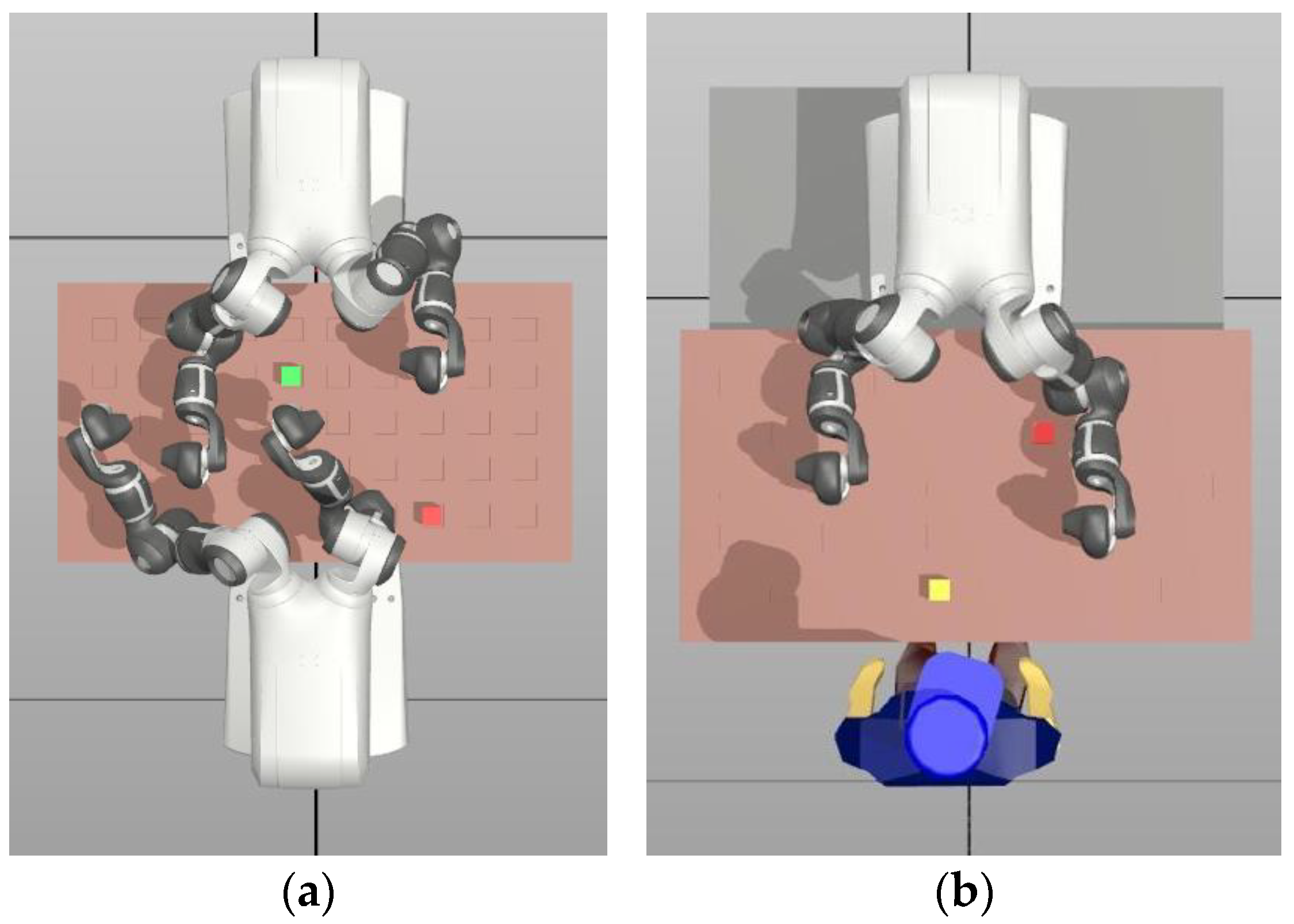
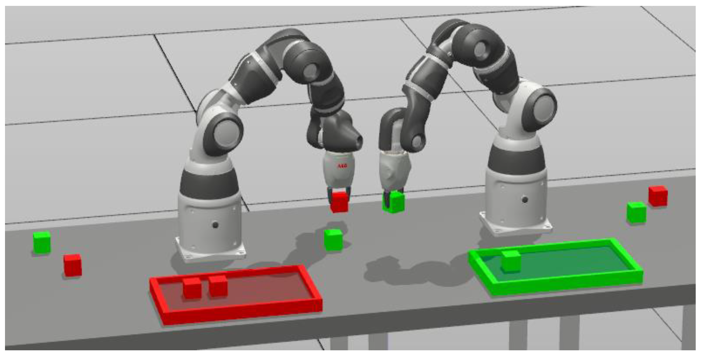
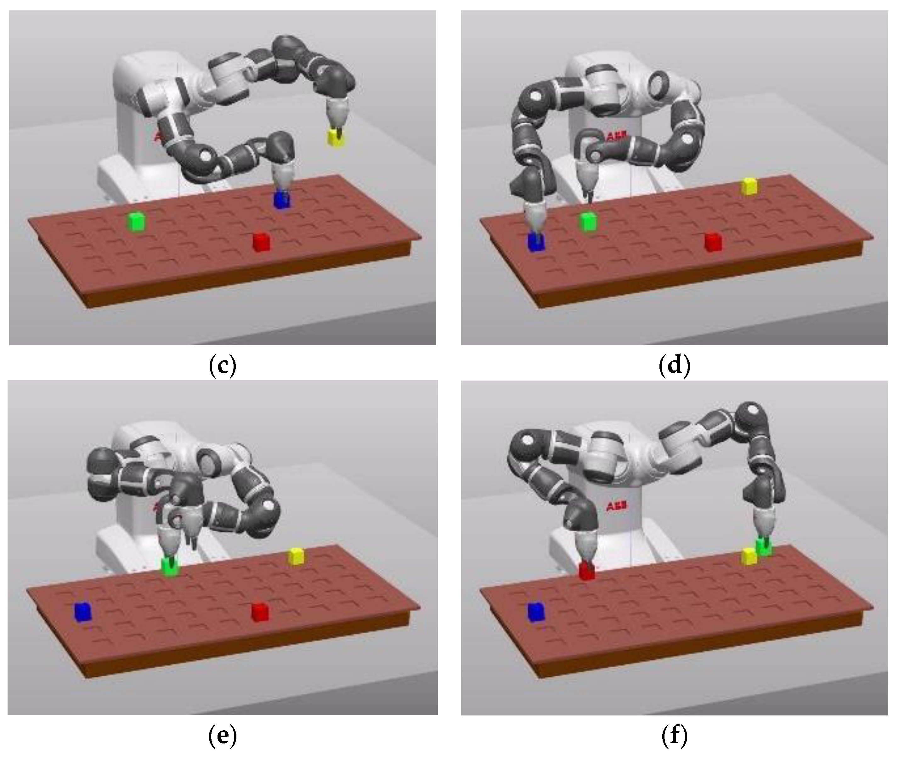
Figure 1 shows a group of robots sharing the same workspace and performing a common pick-and-place task. In this case, the group of robots needs to place pieces of the same color in their corresponding trays without colliding with each other and completing the task as efficiently as possible.
Typically, robot trajectories are programmed to ensure there is no collision between the robot and a static environment. Since robots are often used for repetitive tasks, it is sufficient to plan collision-free trajectories only once. If certain parts of the production process are modified, it becomes necessary to re-plan collision-free trajectories and reprogram all manipulators. In cases where the environment is unpredictable, such as when multiple robots are present, operators modify the workspace, or there are changes in the production process conditions (e.g., the repositioning of production elements), modular approaches are required where each robot can react to changes in real time. The ability to optimally adapt to flexible manufacturing needs, would be an advantage in new production processes.
Object manipulation involves not only performing tasks while avoiding collisions between robots and the environment but also doing so in the shortest possible time.
Figure 2 depicts a representation of a production process where a series of pick-and-place operations need to be performed in a non-predefined order. This means that a certain number of pieces (e.g., kitting operation [
4]) must be manipulated in any order, while considering the establishment of a pick-and-place operation sequence that minimizes the operation time. In this sense, a set of robotic arms, as shown in
Figure 2a, or a dual-arm robot and a human operator, as shown in
Figure 2b, could be considered. This last case is particularly relevant because the system needs to be adapted to the “disappearance” of pieces grabbed by the operator, which entails an instantaneous change from one state to another, requiring the recalculation of the optimal solution.
A particular case, as shown in
Figure 3, is when a specific robot (e.g., left robot) requires the collaboration of another (e.g., right robot) to reach a piece and place it in the desired location. This type of task involves more than just trajectory planning; it requires high-level task planning, which becomes even more complex when a task must be completed in the shortest possible time.
This research introduces a new approach for effectively and efficiently solving pick-and-place tasks by using machine learning algorithms and smart architectural design. It becomes more significant in collaborative scenarios with multiple pieces and multiple robots sharing a common workspace. It plays an automation role, eliminating the requirement for a human to manually create the trajectories for the robots, and placing emphasis on task time minimization. This study shows this approach applied to a scenario comprising multiple pieces, ranging from 2 to 10, and a pair of robots, specifically a collaborative robot with two arms.
This article is organized as follows.
Section 2 provides a brief analysis of the current state-of-the-art in pick-and-place algorithms.
Section 3 describes the proposed approach, formulated as a discretization of the robot’s workspace. The actions that the robot can perform to solve the problem and collision avoidance system are presented.
Section 4 focuses on solving the problem, addressed as a Markov Decision Process (MDP) and as a planning problem using Planning Domain Definition Language (PDDL). The study’s results are presented in
Section 5, where, in addition to demonstrating the algorithm’s performance, the results obtained in a visual environment are shown. Simulations provide an intuitive evaluation of the outcome. Finally,
Section 6 presents the conclusions and proposes future work in this field.
2. Related Work
In recent years, there has been an increasing emphasis on developing algorithms to optimize the pick-and-place task, with a particular focus on minimizing operation time. This challenge has been addressed in different applications, such as shoe production [
5], PCB assembly [
6], and the pick-and-place of individual nanowires in Scanning Electron Microscopy (SEM) [
7]. Previous research has addressed different subproblems related to pick-and-place optimization, including placement sequencing and feeder allocation [
8], among others. Minimizing operation time has been extensively explored in the field using metaheuristic algorithms. Given the complexities associated with these problems, heuristic and metaheuristic algorithms are widely employed to solve them. Examples of such algorithms include Particle Swarm Optimization (PSO) [
9], the Genetic Algorithm (GA) [
10], and Ant Colony Optimization (ACO) [
11]. These methods employ stochastic search techniques that emulate biological or natural evolution and natural selection. One advantage of these methods is that they often provide solutions that are close to optimal in most cases [
12].
Several studies have employed mathematical algorithms in industrial pick-and-place processes. In [
13], an ACO algorithm was proposed, which outperformed the Exhaustive Enumeration Method (EEM), although the study did not specifically address multi-objective pick-and-place processes. GA and ACO algorithms presented better solutions in terms of execution time in pick-and-place problem-solving for PCB assembly, compared to PSO and SFLA algorithms due to their optimized structures [
8]. The Hybrid Iterated Local Search (IHLS) algorithm combines local search and integer programming to drastically reduce computing time for large-scale processes compared to other heuristics. In [
12], a novel metaheuristic algorithm called Best Uniformity Algorithm (BUA) was developed. It generates random solutions within a search space to find the optimal pick-and-place sequence. The BUA algorithm achieved remarkable results in less time when compared to the GA algorithm, although for smaller problem sizes. Its implementation focused on a sequential pick-and-place process involving a single head moving one object at a time. A similar approach was presented in [
5], where a Decision Tree Algorithm optimized the pick-and-place sequence using a two-armed robot to place shoe components into a mold. The Decision Tree Algorithm was employed to recognize patterns and calculate the best real-time optimized sequence. The results indicated that implementing the algorithm improves performance compared to random planning.
While [
14] shares a similar objective, it diverges in terms of approach. This work focuses on collision-free path planning using priority arbitration based on the distance to the goal. However, unlike the referenced work, it does not incorporate prior planning of the operation order to minimize the task execution time. This aspect has been successfully addressed in the algorithm proposed in this article.
4. Solution of the Problem
The problem has been addressed as a decision-making challenge. Reinforcement Learning (RL), a growing field in Artificial Intelligence, is dedicated to this domain, encompassing a wide range of situations, including uncertainty, vast or continuous state and action spaces, the absence of a model, multi-agent environments, and so on. RL necessitates the representation of the model as a Markov Decision Process (MDP).
In this study, the architecture of the system and the model has been defined by design, hence the model is perfectly known, the state and action spaces are discrete, finite, deterministic, and relatively huge, but do not exceed the limits, requiring some kind of function approximator. The architecture is designed such that the controller acts as a single brain for all robots, making it a single agent. Given these properties, methods from other areas, such as graph search or planning languages, may be applied as well.
Figure 7 represents the whole experiment process for all three approaches (MDP, Graph search, and PPDL). The diagram illustrates a sequence of tasks that each approach needs to complete in a specific order. The flow is divided into three stages: Project Level, Task Level, and Execution Level.
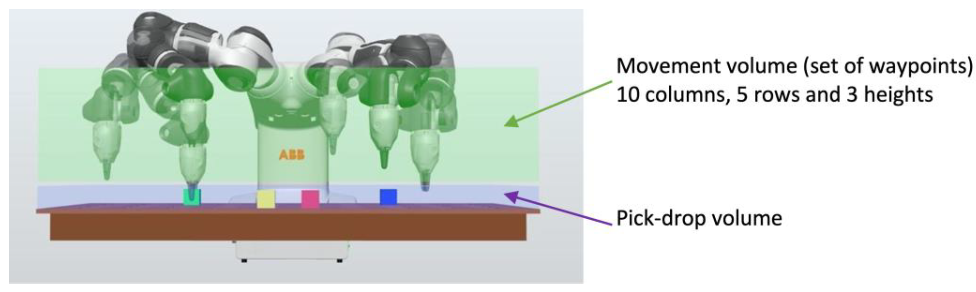
The Project Level stage is common for all approaches and involves any task depending on predefined and invariable design decisions for the project, such as the robot selection (YuMi) or the grid resolution (10 × 5 × 3). This stage needs to be performed only once, unless any of those design decisions change, such as using a new robot. This stage is responsible for generating the system database (described in
Section 3.3.5), which in turn, is an input for the Task Level stage. The database includes information related to robot location feasibility, the robots’ collision, and the robots’ joint configuration.
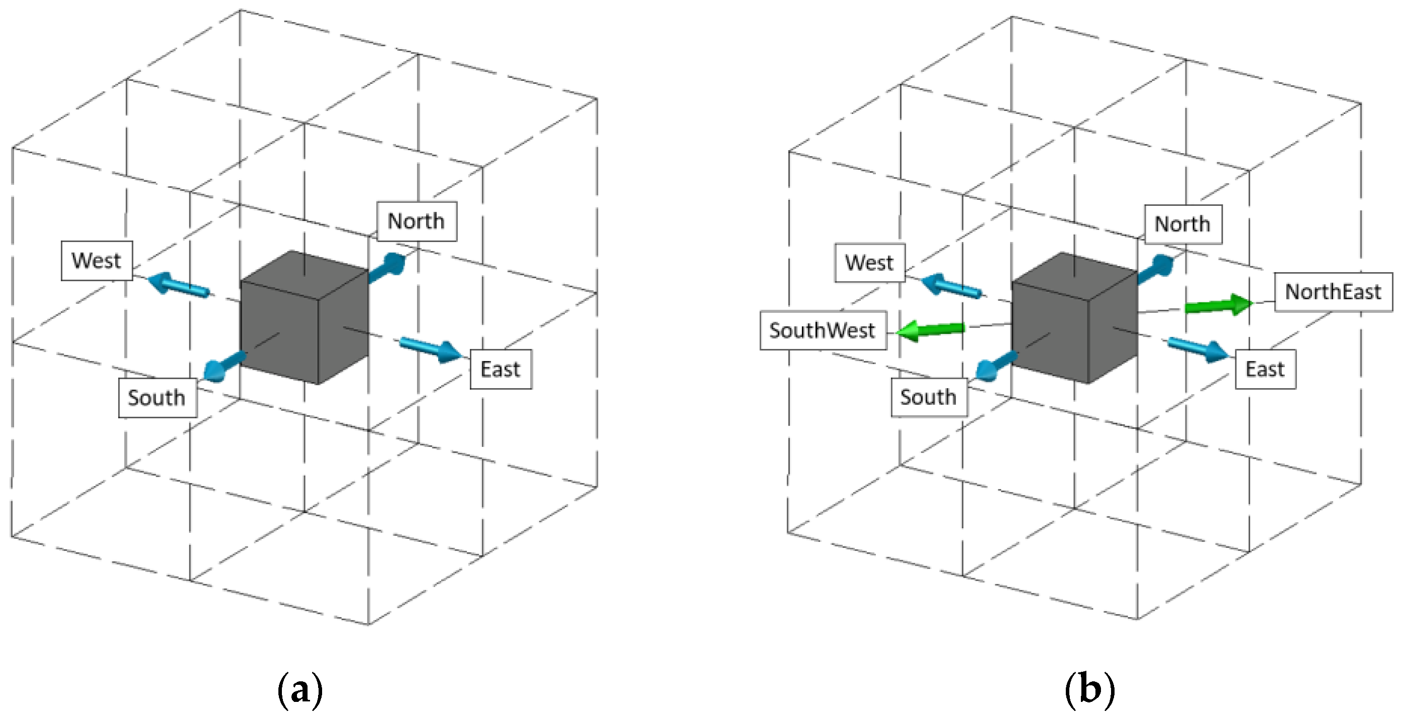
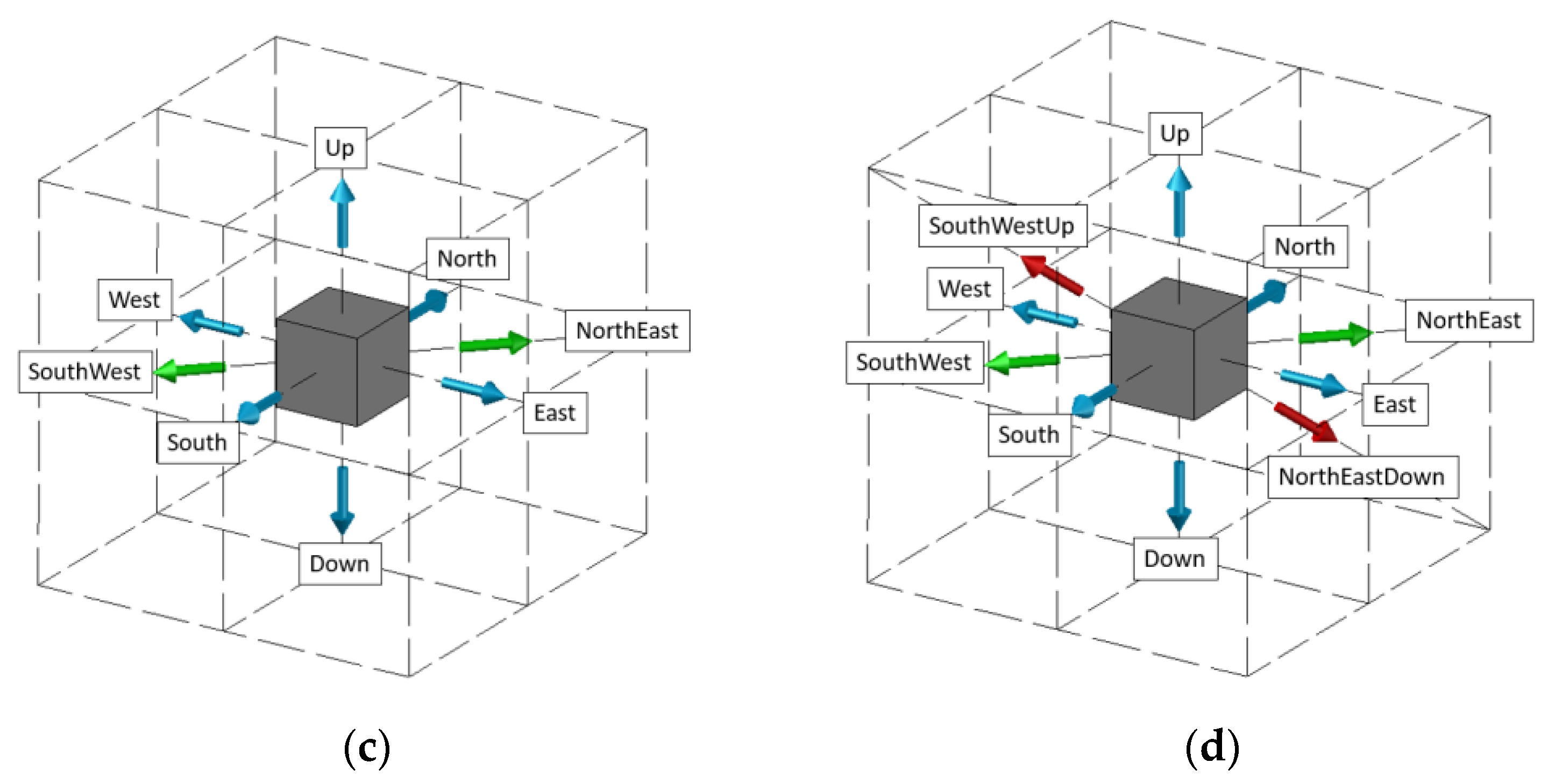
The Task Level stage is related to any task that involves parameter changes in successive experiments. This stage only needs to be re-executed if any of those parameters change. These parameters are the number of available actions, the grid size, and the number of pieces. The number of available actions and the grid size depend on the mode of action (described in
Section 3.3.2) selected for the experiment. While still keeping the same grid resolution (100 mm between cells), some experiments restrict the robot movement to a plane (reducing the grid to 10 × 5 × 1). The number of pieces ranges from 2 to 10. This stage only applies to approaches based on the MDP (MDP and Graph search) and it is responsible for building the MDP model and saving it to disk. This stage is performed offline, and the resulting MDP model is valid for any parameter changes in the next stage.
The Execution Level is also known as the online stage. At this stage, the process receives information about the location of the pieces and robots. The entity providing the location of the pieces is out of the scope of this study. At this stage, the flow for each approach diverges.
The first step in the MDP approach is to update the MDP model. Even though the MDP model is built in the previous stage, the location of the pieces is unknown at that point, hence the state-action pairs related to pick or drop operations need to be updated in this stage once this information is available. MDP generation is split to reduce the online execution time, as most of the computation is performed offline. Once the MDP is built, an MDP solver can be applied to generate a solution. Value Iteration was selected (described in
Section 4.1) for this study.
The first step in the Graph search flow is common with the MDP flow, the MDP model update. Once the MDP is fully defined, there is a conversion task devoted to transforming the MDP model into a graph (described in
Section 4.2). This graph could be solved by any search algorithm. BFS was selected for this study (described in
Section 4.2).
The last flow, PDDL, involves two tasks, the generation of the PDDL source code and generating a solution for the PDDL description. The first task is automated. This automation takes some inputs: the number of pieces, their locations, the robot locations, and the target, and generates the PDDL description for this particular problem. The solution generation is carried out by a PDDL planner solver. FastDownward was selected for this study.
All three approaches converge again in the Task Plan, where a common file format solution is generated. Specifically, for this study, this file contains the sequence of joint configurations and gripper actions required for each robot to complete the overall task.
The final step of the process involves implementing the solution to either a real or simulated problem. In this study, RobotStudio
® was used to simulate the process. RobotStudio
® requires the solution file, the process project (including the robot, the pieces, and the worktable), and the robot source code as inputs. The robot source code is written in RAPID, which is a programming language used for ABB robots. The robot program was used in all experiments to parse the solution file and execute the actions on the robots (see simulation video links in
Section 5.2).
4.1. MDP Model
A Markov Decision Process is a mathematical framework for modeling decision-making problems under uncertainty. The four core components of an MDP model are: a set of states
, a set of actions
, the state transition function
, and the reward function
. The transition function indicates the probability of reaching a state
if an action
is taken in state
. The reward function indicates the reward obtained for that same transition. The key property of an MDP is the Markov property, which states that the effects of an action taken in a state only depend on that state and not on the prior history.
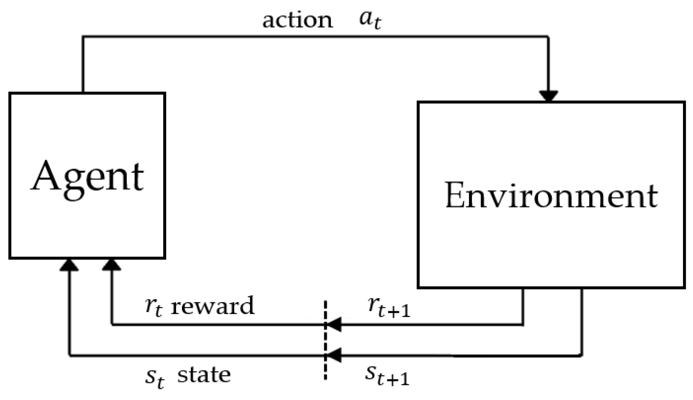
Figure 8 represents this concept, where the next state
and reward
only depend on the current state
and the action taken in it.
In the context of this study, the agent is the brain making decisions, and the environment is the system under control, including the pieces and robots. Depending on the nature of the problem, the MDP may be fully known, partially known (i.e., the reward function is unknown), or totally unknown. In this work, the MDP is totally known (all four core components are defined by design). The state-space and action-space are described in detail in
Section 3.3.2 and
Section 3.3.3, respectively.
The system is deterministic, so the state transition function in this study is not expressed in terms of probabilities , but as a function , which specifies the next state of the system given its current state and the action taken. This component has been modelled in the software implementation as a LookUp Table (LUT), which is indexed by the current state and action and returns the next state. The logic used to populate the table has been implemented in Python and takes all the information into consideration (i.e., the grid boundary exceeded by a robot, collision between robots, location not reachable, invalid action on the current state, etc.).
For the same reason (deterministic system), the reward function is expressed in this study as
instead of
. This component is also modelled as a LUT, and is indexed the same way as the transition function, but it returns the reward value. The logic to populate this LUT is implemented in Python as well. By design, there are three kinds of defined rewards:
A big reward (+100) indicates that the goal is met (all pieces have been transported). A big penalty (−20) indicates that the action taken on the state is not valid (i.e., exceeding grid boundaries, collision between robots, etc.). Finally, a small penalty is applied in all other cases as a strategy for RL algorithms to find the optimal solution (smallest number of steps), since their purpose is to maximize the long-term reward.
The core idea behind this framework is simple. At any point in time, the agent takes an action based on the current system state. As a result, the system state changes, according to the Transition function, and the agent receives a feedback or reward, according to the Reward function.
The purpose of any RL algorithm over an MDP model is to find the optimal action to take on any state. This concept is called Policy, , and based on that policy the agent can make a sequence of optimal decisions from the initial state up to the goal state. Typically, RL algorithms are classified into two groups, model-based and model-free. Unlike model-free algorithms, model-based ones explicitly learn the model (reward and transition functions) of the system, and then apply planning over it. In this work, the model is known, and consequently, only the planning stage is required.
MDP Solver
There are many reinforcement learning algorithms that aim to learn the MDP model either implicitly or explicitly with the goal of finding a good policy [
16]. In this study, the MDP is defined by design, hence there is no need to learn it. In this scenario, finding a good policy is a matter of planning. There are several dynamic programming algorithms that are well suited to this task, such as Value Iteration and Policy Iteration. Value Iteration (VI) was selected for this study.
The Value Iteration core component is called the Value function (V) and represents, for any given state
, the expected cumulative reward from that state
to the goal state, following a certain policy
. Initially, the policy
is usually arbitrary, so the Value function
presented in Equation (5) is not a good estimation of the cumulative reward. The aim of Value Iteration is to find a policy that maximizes V, which is known as
presented in Equation (6).
Indeed, it is an iterative algorithm, where
is gradually improved on each iteration by applying the Bellman equation presented as (7).
The General Bellman equation may be simplified for deterministic environments when using additive discounting (a small negative reward for moving to non-terminal states). Under this scenario, the multiplicative discount (discount factor) may be set to 1, and the expression is reduced to its simplest form, as seen in (7).
The algorithm stops when
converges to
, since the Value function is not going to improve anymore, that is, the
matrix will remain the same on additional iterations. In practice, the algorithm usually stops when the variation in
is less than a certain predefined threshold. At this point, the optimal policy
can be directly derived from
and it is presented in Equation (8).
Applying the same reasoning as in (7), the discount factor is set to 1 in (8). is used to model the uncertainty in the environment. The system in this study is deterministic, hence there is only one state out of the whole state-space with a probability bigger than 0 (actually, probability 1). Under this scenario, this term can be removed, and the expression is reduced to its simplest form, as seen in (8).
It is worth noting the optimal is unique, but there might be multiple leading to this optimal Value function. This means that different sequences of actions might lead to the same result. This has a direct impact on this problem, specifically in the situation where a robot has nothing else to do (i.e., there are two robots and only one piece left).
The implementation of this algorithm was written in Python. The simplified Bellman Equation (7) was expressed in matrix form, and the matrix computations were performed using a numerical library called NumPy. Once the Value function has converged, the optimal policy is obtained using the simplified policy Equation (8).
From the point of view of the algorithm, it is irrelevant if one of the robots is idle or randomly moving. In practice, it is usually preferred that this robot keeps idle. To tackle this point, a smart ordering of the system actions was performed (system actions that affect only one robot’s movement have priority over those in which both robots move), so in case of multiple actions leading to the same result, the preferred one will be returned by the argmax operation in Equation (8).
4.2. Graph Model
In this approach, the system model was represented as a graph. Specifically, the graph was directly derived from the matrix version of the MDP model (transition and reward functions) described in
Section 4.1. A graph basically consists of three types of elements: nodes, transitions, and costs. There is a direct mapping between MDP states and graph nodes, and between MDP state transitions and graph node transitions. Graph costs are derived from the MDP rewards, although the mapping is not direct and specific transformations have been performed. The resulting graph is a reduced version of the MDP model that incorporates the following reward-cost transformations, as shown in
Table 1.
All invalid state-action pairs (i.e., an action in a specific state results in exceeding the grid boundaries) have not been included in the graph. The small penalty (−1) reward in the MDP is transformed as a small positive reward (+1), since the target of a graph search algorithm is to minimize the path cost, unlike MDP-based algorithms where their target is to maximize the long-term reward.
Finally, all direct-to-goal transitions in MDP (transitions from state to where is a goal state) have the same reward value (+100). The Graph search algorithm’s target is to minimize the path cost, and the key point is that every solution (optimal or not) will include one and only one of those direct-to-goal transitions (the very last transition in the path). Based on that property, any arbitrary cost value would be valid for those transitions as long as all of them keep the same value. The cost value chosen for those transitions is +1, resulting in a graph where all costs are the same value (unweighted graph).
Graph Search
There is a wide range of graph search algorithms. Commonly, they are classified as informed search algorithms (i.e., Dijkstra [
17] or A* [
18]) or uninformed search algorithms (i.e., BFS [
19] or DFS [
20]). Uninformed search algorithms explore the state space in a blind manner, while informed search algorithms take advantage of additional information (such as the transition cost values) to guide and reduce the state-space exploration.
Given the characteristics of the current graph model, where all the costs have the same value, which is equivalent to say that there is no information at all to guide the search, an informed search algorithm does not provide any advantage over an uninformed search one. Moreover, under this specific scenario, an uninformed search implementation is easier and lighter, resulting in slightly better execution times. The BFS (uninformed search) algorithm was selected for this approach.
BFS is an algorithm used to explore a graph or a tree-like data structure. BFS guarantees to find an optimal solution if the graph is finite and deterministic [
21]. The graph representing the system in this work meets those properties. Additionally, it is an unweighted graph, hence the computational cost might be further reduced since the algorithm can be stopped at the depth level where the first solution is found. Any solution found on a deeper depth level would imply a path with more actions involved.
It is worth noting that the common mental representation of a graph solution is the shortest path between two points, seen as a physical distance magnitude. Actually, the path between two nodes may involve multiple concepts other than physical distance. In this study, the shortest path between the node representing the initial state of the system and the node representing the goal state includes all kinds of trajectories carried out by every robot, the optimal assignment of the pieces, the order in which they are processed, etc.
The main language used for the implementation of this study was Python. Generally, a Python application is not as efficient as one written in a compiled language, such as C. On the other hand, Python supports using modules written in other languages, such as NumPy [
22], a very optimized numerical library written in C. The Value Iteration algorithm described in
Section 4.1 was implemented in Matrix form, taking advantage of the NumPy matrix operations. In order to enable a fair comparison between algorithms, BFS was implemented in C as well, and imported in Python as a module. Its pseudo-code can be seen in Algorithm 3.
| Algorithm 3: Pseudo-code to implement Breadth First Search algorithm. |
1: BFS (G, s) // Where G is the graph, and s is the source node 2: let Q be the FIFO queue. 3: // Inserting s in queue 4: Q.enqueue(s) 5: mark s as visited 6: // Loop until the queue is empty 7: while (Q is not empty) 8: // Remove the first node from the queue 9: v = Q.dequeue 10: // Process all its neighbors 11: for all neighbors w of v in Graph G 12: if w is not visited 13: // Insert w in Q 14: Q.enqueue(w) 15: end if 16: end for 17: end while
|
4.3. Planning Domain Definition Language
Planning Domain Definition Language (PDDL) is an attempt to standardize Artificial Intelligence (AI) planning languages. PDDL has a variety of versions, such as Probabilistic PDDL (PPDDL) [
23] to account for uncertainty, Multi-Agent PDDL (MA-PDDL) to allow planning for multiple agents, etc. In this study, the problem was designed as single-agent and deterministic, so the official PDDL language was used. PDDL models the problem in two separate files: the Domain file and the Problem file. The Domain file contains the predicates and actions; predicates are facts of interest, such as “is
i robot in XYZ location?”, “is there collision in the current state?”, and “is
i robot carrying the piece
j?”, and those predicates are evaluated as true or false; actions are the counterpart of the transition function in the MDP model; that is, the way the system state changes. The Problem file contains the initial state, the goal specification, and the objects; the initial state and goal specification are straightforwardly associated with the initial and goal state in the MDP model; the objects are the counterpart of the internal variables of the MDP model (robot location, robot status, and piece status).
Unlike MDP or graph search methods, this approach ends with the model problem definition. Then a well-proved software planner is used to obtain a solution. Some of the most used planners are FastDownward [
24], LPG [
25], and PDDL.jl [
26]. In this project, FastDownward was used. FastDownward is a planner that relies on a heuristic search to address several planning problems, including PDDL. It is recognized as one of the most efficient planners currently available. Unlike other planners, FastDownward employs an alternative translation known as “multivalued planning tasks” instead of using the propositional representation of PDDL. This approach significantly enhances search efficiency.
6. Conclusions and Future Work
This article presents a method to coordinate robotic manipulators, avoiding collisions between arms during pick-and-place operations, and minimizing the task time by selecting the best manipulation sequence and the best trajectory planning. Due to the assumed simplifications in the system (deterministic, single-agent, and fully observable), the Markov Decision Process (MDP) proposed can be transformed into a graph that can be solved using a search algorithm, such as Breadth First Search (BFS). Additionally, the Planning Domain Definition Language (PDDL) has been used to generate an alternative solution that can be compared with VI and BFS.
For every test case where a solution can be obtained, all three algorithms consistently produce an optimal solution, which is not unique and may differ between all algorithms. In this context, optimal refers to the least number of steps required to complete the task. Regarding the computational cost to find a solution, the graph search method (BFS) turns out to be the fastest one, although limited in terms of scalability. In fact, the generated graph is derived from the MDP model, so actually both MDP and BFS approaches suffer this same scalability issue, directly related to the number of pieces and robots. On the other hand, the PDDL scales better and is able to solve all tested cases. The MDP approach is neither the fastest nor the least eager on resources, but provides a general framework capable of scaling to more complex problems, including uncertainty, the continuous state and action spaces, the partially observable state, etc. The last factor, irrespective of the algorithm used, is the flexibility of the robot’s navigation. A significant enhancement of the solution is observed when diagonal movements are incorporated into the 2D plane (as outlined in Mode 2 in
Section 3.3.2). While the inclusion of extra movements for 3D space navigation results in a marginal improvement in the solution, it comes at a substantial expense due to the computational cost being exponential to the number of robots (in this case, quadratic, as there are two robots).
However, the proposed method has several disadvantages. Firstly, the system does not scale well. The provided solution is feasible for certain production processes where the number of pieces to manipulate is small (less than 10 elements). Secondly, the movements that the robots must perform are constrained within a grid, which is less natural compared to other solutions such as [
15], although it provides a robust and faster industrial solution to the problem. Lastly, a preliminary study using RobotStudio
® is required to create a database, including information about collision situations between arms.
In future work, the intention is to explore new techniques, such as hierarchical reinforcement learning or multi-agent learning, that can overcome the scalability limitation of the current single-agent approach. The goal is to introduce a larger number of pieces and robots that could operate within the same workspace. Another objective is to investigate alternative implementation strategies, such as using specialized HW (GPU), since the algorithm (VI) core is heavily based on matrix operations. Additionally, the preliminary study of robot collisions demands considerable time and complexity. Therefore, an alternative method is being considered. A possible solution is to frame the robot links within a set of ellipsoids and check for collisions between these ellipsoids in space. This approach would eliminate the need to rely on a graphical environment such as RobotStudio®, reducing offline computational costs but potentially increasing online computational requirements. Hence, an analysis of the performance of this new approach would be required.


