Article

Patterns Simulations Using Gibbs/MRF Auto-Poisson Models

Department of Statistics and Actuarial-Financial Mathematics, University of the Aegean, 83200 Karlovassi, Greece
Technologies 2022, 10(3), 69; https://doi.org/10.3390/technologies10030069
Submission received: 14 April 2022 / Revised: 28 May 2022 / Accepted: 2 June 2022 / Published: 6 June 2022
(This article belongs to the Special Issue 10th Anniversary of Technologies—Recent Advances and Perspectives)

Abstract

:
Pattern analysis is the process where characteristics of big data can be recognized using specific methods. Recognition of the data, especially images, can be achieved by applying spatial models, explaining the neighborhood structure of the patterns. These models can be introduced by Markov random field (MRF) models where conditional distribution of the pixels may be defined by a specific distribution. Various spatial models could be introduced, explaining the real patterns of the data; one class of these models is based on the Poisson distribution, called auto-Poisson models. The main advantage of these models is the consideration of the local characteristics of the image. Based on the local analysis, various patterns can be introduced and models that better explain the real data can be estimated, using advanced statistical techniques like Monte Carlo Markov Chains methods. These methods are based on simulations where the proposed distribution must converge to the original (final) one. In this work, an analysis of a MRF model under Poisson distribution would be defined and simulations would be illustrated based on Monte Carlo Markov Chains (MCMC) process like Gibbs sampler. Results would be illustrated using simulated and real patterns data.

1. Introduction

Pattern analysis is a class of methods that are used to recognized regular patterns in big data, like images. Considering these methods, models must be introduced, and analysis of the modeling process must be performed. Especially for the images, the spatial structure of the pixels is an important measure to explain the spatiality of the image.
Spatial structure of images can be analyzed based on specific models, where neighborhood structures are taking into consideration. Interactions between regions at different scales are characterized by their local dynamics, and the emergent spatial patterns are the outcome of different processes. Local dynamics could be explained by the local characteristics of the image with the main result being the construction of the images under homogeneous regions. The homogeneity of the image could be defined by the spatial pattern of the image, which is explained with way better presentation of real data. Under these local characteristics, special models considering the neighborhood structure of the image could established specific conditional models defined as Markov Random fields (MRF) models. These models are defined by Markov Random fields (MRF) models, explaining the spatial structure of the images by a conditional distribution of the pixels, defined as auto-models. These models under appropriate structure patterns have the ability to explain real patterns. Under the conditional distribution, various models could be introduced. In our work, the specific class of data that can be analyzed as best as it can is based on the Poisson distribution, defined as auto-Poisson models.
Referring to conditional probabilities, due to the largeness of the configuration space, it is impractical to sample from it by direct computation of the probabilities. Markov chains Monte Carlo (MCMC) methods have been investigated by various researchers as an alternative to exact probability computation [1,2]. The general method is to simulate a Markov chain with the required probability distribution as its equilibrium distribution. If the chain is aperiodic and irreducible, the convergence is guaranteed.
The main goal is to introduce a method where a model can be defined and investigated. Based on this investigation, characteristics for this model (auto-Poisson) can be held and generalized for similar image patterns. Simulations of the process are achieved by using MCMC method, like Gibbs sampler, in simulated and real data.

2. Materials and Methods

Markov Random Fields Modeling

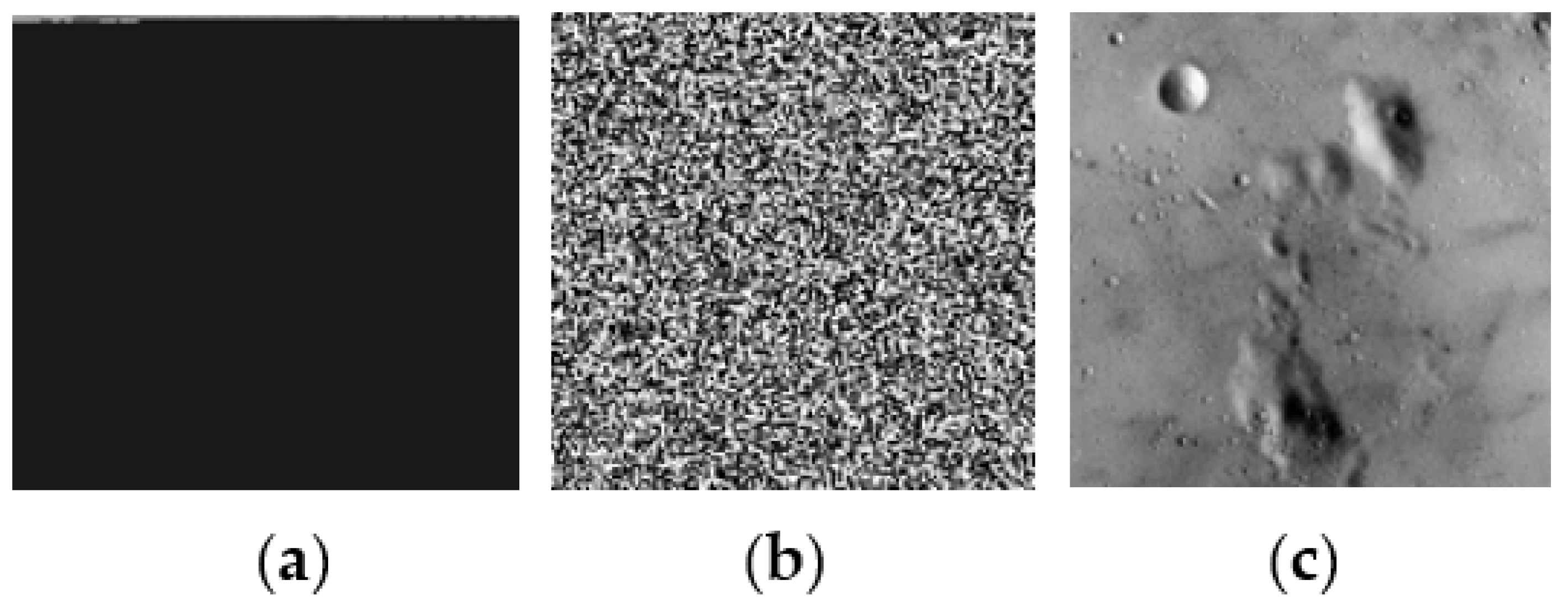
Spatial data under investigation can be defined as regular or irregular areas (Figure 1). Under these areas, spatial patterns cam be illustrated based on the structure of the images. The main goal is to model the spatial patterns in a way to represent as best as they can the real data starting from a simple model to a more complicated one (Figure 2).
Considering a 2-D space, which has been partitioned into n-pixels, labeled by the integers 1, 2, …n (rectangular space); xij or xi denote the color for pixel (i) or (i,j); p(..|..) defined as the conditional probability distribution (Figure 3) ([3,4,5,6]).
If D is a finite lattice D = {(i, j), 1 ≤ i ≤ N, 1 ≤ j ≤ M}, then each pixel of the finite lattice D can be colored from the set {0, 1,…,c − 1}. Site j (1 i) is said to be a neighbor of site i iff the functional form of p (xi|x1,…, xi−1, xi+1,…, xn) is defined upon the variables xj as p ( x i | x 1 , , x i 1 , x i + 1 , , x n ) = p ( x i | x i ) , where ∂i is the set of pixels that are neighbous of pixel I, and x∂i is the set of values of pixels that are neighbors of pixel i.
A neighborhood structure N = {Ni, i S} is defined as a collection of subsets of S. The symmetry property is based on the following conditions: (i) i ∉ Ni (a site is not part of its neighborhood); (ii) j ∈ Ni ⇔ i ∈ Nj (i is in the neighborhood of j if and only if j is in the neighborhood of i). Define a nearest-neighborhood set as the set of sites with the property that p (xij|all other values) depends only upon the neighbors xi−1,j, xi+1,j, xi,j−1, xi,j+1 for each internal site (i,j) (Figure 4).
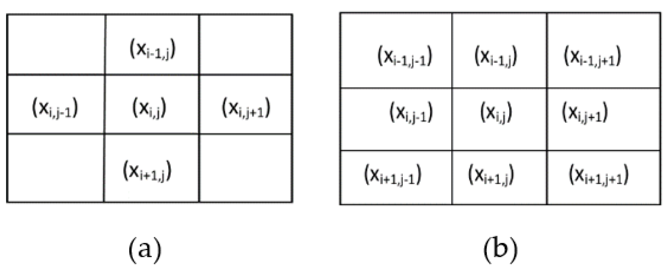
The first order model (four neighbors) is denoted by N = {(xi,j, xi−1,j), (xi,j, xi+1,j), (xi,j, xi,j−1), (xi,j, xi,j+1)} and second order (eight neighbors) is denoted by N = {(xi,j, xi−1,j), (xi,j, xi+1,j), (xi,j, xi,j−1), (xi,j, xi,j+1), (xi,j, xi−1,j−1), (xi,j, xi−1,j+1), (xi,j, xi+1,j−1), (xi,j, xi+1,j+1)} (Figure 5).
A clique is defined as a set that consists either of a single pixel or a collection of pixels that are neighbors of each other. Given a 2-D space of a subset S and neighbor structure ∂i, a clique is any set of pixels c ⊂ S, where for all i, j ∈ c, j ∈ ∂i. C can be defined as the set of all cliques. The concept of clique is directly combined with the calculation of the energy of the image, which can be considered as a statistical measure of the weight of the correlation between the pixels.
For the first order, the neighborhood structure is given by: {(i,j)}, {(i − 1,j), (i,j)}, {(i,j − 1), (i,j)}; and for the second order the neighborhood structure is given by: {(i,j)}, {(i − 1,j), (i,j)}, {(i,j − 1), (i,j)},{(i − 1,j − 1), (i,j)}, {(i − 1,j + 1), (i,j)}, {(i,j + 1), (i − 1,j + 1), (i,j)}, {(i,j + 1), (i − 1,j), (i,j)}, {(i − 1,j − 1), (i − 1,j), (i,j)}, {(i − 1,j + 1), (i − 1,j), (i,j)}, {(i − 1,j − 1), (i − 1,j + 1), (i + 1,j + 1), (i + 1,j − 1),(i,j)}.
A Markov random field (MRF) is a joint probability density on the set of all possible coloring values X on a finite lattice D, following the conditions ([3,4,7]): (i) p (x) > 0 for all x ∈ S. (Positivity). (ii) p (xij|all points (i,j)) = p (xij|neighbors). (Markovianity). (iii) p (xij|neighbors (i,j)) depends only on the configuration of the neighbors (Homogeneity). The probabilities on the condition (2) are called local characteristics. Condition (2) can be expressed as p ( x i | x j , i j ) = p ( x i | x i ) , where it is clear that we need a representative distribution (Gibbs). If p (x) is a jpdf of Χi ∈ S under any neighborhood model ∂i, the Gibbs distribution can be expressed based on the following form:
p ( x ) = 1 Z exp { 1 T [ U ( x ) ] } = 1 Z exp { 1 T [ c C V c ( x c ) ] }  
where C are all the potential cliques, Ζ is the normalized constant/partitions function, Τ is is the temperature with Τ = 1, and U (x) is the energy function with U ( x ) = c C V c ( x c ) [8]. Under the Hammersley–Clifford theorem ([9,10]), if X is a discrete or continuous variable assigned to a pixel x representing a random field with neighborhood structure ∂i and jpdf p (x), then Χ is a MRF. iff p (x) can be expressed as a Gibbs distribution. The general form for the energy function can be defined by
U ( x ) = i S V 1 ( x i ) + i S j S V 2 ( x i , x j ) = 1 i S x i G i ( x i ) + 1 i < j S x i x j G i j ( x i , x j ) + ....  
where G (.) is any arbitrary function ([3,4]). For example, for the second order neighborhood structure, the energy function is given by
U ( x ) = i S V 1 ( x i ) + i S j S V 2 ( x i , x j ) = 1 i S x i G i ( x i ) + 1 i < j S x i x j G i j ( x i , x j )  
defined as pairwise interaction MRF models.
Specific spatial patterns can be described by particular models based on their neighbors, defined as auto-models. Assumptions for these models are: (1) The probability structure only depends on contributions of sites taken either as singular or in pairs. (2) The conditional probability distribution is a member of the regular exponential family of distributions p ( x i | x i ) = exp { A i ( θ i ) B i ( x i ) + C i ( x i ) + D i ( θ i ) } where θi is a model parameter associated with site i and is a function of the values at sites neighboring site i. Aii) can be defined as a potential interaction between pixels. Assuming the conditional probabilities and the pairwise only dependence between sites, the Aii) must satisfy ([2,5,6]):
A i ( θ i ) = α i + β i j B j ( x j )  
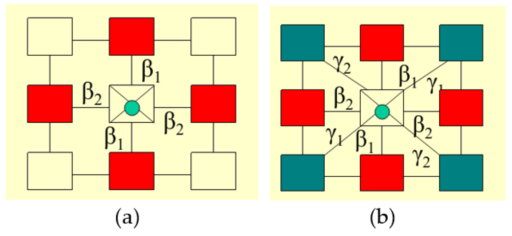
where βij = βji if i is neighbors with j and βij = 0 otherwise. As a final restriction, it is assumed that the function Bj (xj) is linear in xi with form A i ( θ i ) = α i + β i j x j . If βij = βji = β, it is an isotropic model, otherwise it is anisotropic. For the first-order system the models are: isotropic: Ai (α,β) = α + β (xi−1,j + xi+1,j + xi,j−1 + xi,j+1) and anisotropic: Ai (α, β12) = α + β1 (xi−1,j + xi+1,j) + β2 (xi,j−1 + xi,j+1) (Figure 6a). For the second order, the models are: isotropic: Ai (α, β, γ) = α + β (xi−1,j + xi+1,j + xi,j−1 + xi,j+1)+γ (xi−1,j−1 + xi−1,j+1 + xi+1,j−1 + xi−1,j+1) and for anisotropic: Ai (α, β1, β2, γ1, γ2) = α + β1 (xi−1,j + xi+1,j) + β2 (xi,j−1 + xi,j+1) + γ1 (xi−1,j−1 + xi−1,j+1) + γ2 (xi+1,j−1 + xi−1,j+1) (Figure 6b) ([8]).
Considering the general notation of the auto-models, the potential interaction between pixels for the auto-Poisson model is given by
A i ( λ i ) = log ( λ i ) λ i = exp ( a i + β i j x j )  
under the assumption that the conditional distribution of the pixels xi given their neighbors has a Poisson distribution mean λi with form
p ( x i | x i ) = λ i x i exp ( λ i ) x ! = exp [ log ( λ i ) x i λ i log ( x i ! ) ]  
The limitation of the model is that | b | > 1 λ i ([2,5,6]), where b = mβc, c denotes number of colors, and m denotes the number of neighbors.

3. Results

Simulation Process Using MCMC Method

The investigation of the spatial patterns can be illustrated by the simulation procedures. A particular simulation process, where realizations from pseudo-samples can finally define the desired distribution, is the Monte Carlo Markov Chain (MCMC) ([11]). The goal of the process is to simulate the distribution p (x) using a particular realization X1, X2,…, XN on the Markov chain with transition probability. Under the process, asymptotic results can be archived where:
X t t d X ~ p ( x )   ;   1 t i = 1 t f ( x i ) t E p { f ( x ) }
with the expectation Ep {f (x)} under estimation. The corresponding empirical average will be given by
f ¯ N = 1 N t + 1 N f ( x ( t ) )
Gibbs sampler is a special case of MCMC methods. Consider Χi ∈ S a discrete or continuous value for a random field in a rectangular lattice system S with neighborhood structure ∂i. If X is defined as a pdf p (x) based on Gibbs distribution, then the conditional probability of a value given its neighbors can be defined as
p ( x s | x j , s j ) = exp { U ( x s | x j , s j ) } x s * S exp { U ( x s * | x j , s j ) }
Each value could be replaced by the conditional probability
p ( x s | x j k , j s ) = p ( x s | x s )
The algorithm stopped when all the pixels were replaced. The Gibbs sampler algorithm is given by the following pseudo-algorithm ([12,13,14,15]):
Step 1: Chose randomly pixel xi
Step 2: For t = 0 until ∞
Replace the value x(t) with x(t+1) based on
X t t d X ~ p ( x )   ;   1 t i = 1 t f ( x i ) t E p { f ( x ) }
Step 3. Continue the process until all the pixels have been replaced
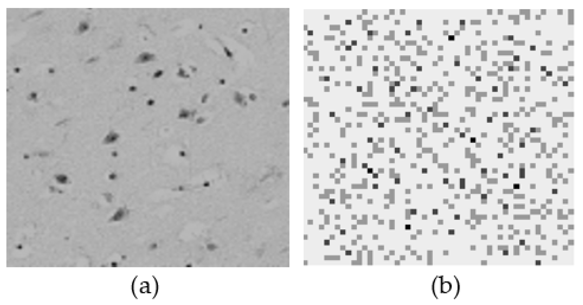
Realizations for the auto-Poisson model are given in Figure 7 with parameter a. First order isotropic with α = 0.75 and β = −0.25; b. Second order isotropic with a = −0.93, β = −0.33, and γ = −0.37. Finally a comparison between biological images from microscopes with realizations from the simulated auto-Poisson model considering the first-order isotropic model (α = −1, β = −2) is given in Figure 8, where it is clear that both images have similar patterns.

4. Conclusions

Pattern analysis is a process where regular synthesis or patterns can be recognized. Most of the time, these patterns can be analyzed using texture models based on the spatial structure of the images. The spatiality of the images can be defined by considering the homogeneity of the regions. These regions might be represented by considering identity patterns under the neighborhood structure of the image. Models for the estimation of these spatial patterns could be introduced considering the local characteristics of the image, leading us to Markov random fields (MRF) models. These patterns could be used to simulate real phenomena like biology, ecology, or medicine. In this work, a presentation of Markov random field models (MRF) considering specific conditional distributions like auto-models was analyzed. A specific auto-model under Poisson distribution (auto-Poisson) were defined and simulations using MCMC methods as Gibbs samples were illustrated using simulated and real images patterns. Modification of auto-Poisson models was successfully performed in many case like social networks [16], spreading disease modeling [17,18], ecological models [19,20,21,22]. In these works, extensions of Markov random fields (MRF) models were applied using network analysis considering the neighborhood structure of the pixels. Under this extension, homogeneous regions could be illustrated considering the connections between similar pixels. Another important application is based on the mapping analysis where simulations of auto-Poisson models might be used to reconstruct estimated maps under various regions, analyzing phenomena like cancer diseases [23]. Last but not least, the proposed models could be used for firm location analysis [24] to estimate the optimal positions for firm’s establishment.

Funding

This research received no external funding.

Institutional Review Board Statement

Not applicable.

Informed Consent Statement

Not applicable.

Data Availability Statement

Not applicable.

Conflicts of Interest

The author declare no conflict of interest.

References

  1. Zimeras, S.; Matsinos, Y. Modeling Uncertainty based on spatial models in spreading diseases: Spatial Uncertainty in Spreading Diseases. Int. J. Reliab. Qual. E-Healthc. 2019, 8, 55–66. [Google Scholar]
  2. Aykroyd, R.G.; Zimeras, S. Inhomogeneous prior models for image reconstruction. J. Am. Stat. Assoc. 1999, 94, 934–946. [Google Scholar]
  3. Besag, J. Spatial interaction and the statistical analysis of lattice systems. J. R. Stat. Soc. 1974, 36, 192–236. [Google Scholar]
  4. Besag, J. On the statistical analysis of dirty pictures. J. R. Stat. Soc. 1986, 48, 259–302. [Google Scholar]
  5. Zimeras, S. Statistical Models in Medical Image Processing. Ph.D. Thesis, Leeds University, Leeds, UK, 1997. [Google Scholar]
  6. Zimeras, S.; Georgiakodis, F. Bayesian models for medical image biology using Monte Carlo Markov Chain techniques. Math. Comput. Modeling 2005, 42, 759–768. [Google Scholar]
  7. Cross, G.R.; Jain, A.K. Markov Random Field Texture Models. IEEE Trans. Pattern Anal. Mach. Intell. 1983, 5, 25–39. [Google Scholar] [CrossRef]
  8. Zimeras, S. Spreading Stochastic Models Under Ising/Potts Random Fields: Spreading Diseases. In Quality of Healthcare in the Aftermath of the COVID-19 Pandemic; IGI Global: Hershey, PA, USA, 2022; pp. 65–78. [Google Scholar]
  9. Hamersley, J.A.; Clifford, P. Markov fields on finite graphs and lattices. 1971, unpublished work.
  10. Kindermann, R.; Snell, J.L. Markov Random Fields and Their Applications; American Mathematical Society: Providence, RI, USA, 1980. [Google Scholar]
  11. Hastings, W.K. Monte Carlo simulation methods using Markov chains, and their applications. Biometrika 1970, 57, 97–109. [Google Scholar]
  12. Geman, S.; Geman, D. Stochastic relaxation, Gibbs distributions, and Bayesian restoration of images. IEEE Trans. Pattern Anal. Mach. Intell. 1984, 6, 721–741. [Google Scholar]
  13. Green, P.J.; Han, X.L. Metropolis Methods, Gaussian Proposals and Antithetic Variables. In Stochastic Models, Statistical Methods, and Algorithms in Image Analysis. Lecture Notes in Statistics; Barone, P., Frigessi, A., Piccioni, M., Eds.; Springer: New York, NY, USA, 1992; Volume 74. [Google Scholar] [CrossRef]
  14. Metropolis, N.; Rosenbluth, A.; Rosenbluth, M.; Teller, A.; Teller, E. Equations of state calculations by fast computing machines. J. Chem. Physics 1953, 21, 1087–1091. [Google Scholar]
  15. Smith, A.F.M.; Robert, G.O. Bayesian computation via the Gibbs sampler and related Markov chain Monte Carlo methods. J. R. Stat. Soc. B 1993, 55, 3–23. [Google Scholar]
  16. Agaskar, A.; Lu, Y.M. Alarm: A logistic auto-regressive model for binary processes on networks. In Proceedings of the IEEE Global Conference on Signal and Information Processing, Austin, TX, USA, 3–5 December 2013; pp. 305–308. [Google Scholar]
  17. Kaiser, M.S.; Pazdernik, K.T.; Lock, A.B.; Nutter, F.W. Modeling the spread of plant disease using a sequence of binary random fields with absorbing states. Spat. Stat. 2014, 9, 38–50. [Google Scholar] [CrossRef]
  18. Shin, Y.E.; Sang, H.; Liu, D.; Ferguson, T.A.; Song, P.X.K. Autologistic network model on binary data for disease progression study. Biometrics 2019, 75, 1310–1320. [Google Scholar] [CrossRef]
  19. Zimeras, S.; Matsinos, Y. Spatial Uncertainty. In Recent Researches in Geography, Geology, Energy, Environment and Biomedicine; WSEAS Press: Kerkira, Greece, 2011; pp. 203–208. [Google Scholar]
  20. Zimeras, S.; Matsinos, Y. Modelling Spatial Medical Data. In Effective Methods for Modern Healthcare Service Quality and Evaluation; IGI Global: Hershey, PA, USA, 2016; pp. 75–89. [Google Scholar]
  21. Zimeras, S.; Matsinos, Y. Bayesian Spatial Uncertainty Analysis. In Energy and Environment; Recent Researches in Environmental and Geological Sciences, Proceedings of the 7th International WSEAS International Conference on Energy & Environment, Kos Island, Greece, 14–17 July 2012; WSEAS Press: Kerkira, Greece, 2012; pp. 377–385. [Google Scholar]
  22. Aykroyd, R.; Haigh, J.; Zimeras, S. Unexpected Spatial Patterns in Exponential Family Auto Models. Graph. Model. Image Process. 1996, 58, 452–463. [Google Scholar] [CrossRef]
  23. Morales-Otero, M.; Núñez-Antón, V. Comparing Bayesian Spatial Conditional Overdispersion and the Besag–York–Mollié Models: Application to Infant Mortality Rates. Mathematics 2021, 9, 282. [Google Scholar]
  24. Brown, J.P.; Lambert, D.M. Extending a smooth parameter model to firm location analyses: The case of natural gas establishments in the United States. J. Reg. Sci. 2016, 56, 848–867. [Google Scholar] [CrossRef]
Figure 1. Different type of areas: (a) lattice; (b) hexagonal; and (c) hive.
Technologies 10 00069 g001
Figure 2. Various types of image models: (a) simple; (b) complicated; (c) very complicated.
Technologies 10 00069 g002
Figure 3. Definition of the 2-D space for image presentation.
Technologies 10 00069 g003
Figure 4. Nearest-neighborhood system.
Technologies 10 00069 g004
Figure 5. Neighborhood structure. (a) first order and (b) second order.
Technologies 10 00069 g005
Figure 6. (a) First-order models and (b) second-order models.
Technologies 10 00069 g006
Figure 7. Realizations from auto-Poisson models: (a) first-order isotropic; (b) second-order isotropic.
Technologies 10 00069 g007
Figure 8. Patterns comparison between real image and simulated image under first order. Isotropic auto-Poisson model: (a) Real image and (b) Simulated image.
Technologies 10 00069 g008
Publisher’s Note: MDPI stays neutral with regard to jurisdictional claims in published maps and institutional affiliations.