Abstract
A digital elevation model (DEM) represents the topographic surface of the Earth and is an indispensable source of data in many applications, such as flood modeling, infrastructure design and land management. DEM data at high spatial resolution and high accuracy of elevation data are not only costly and time-consuming to acquire but also often confidential. In this paper, we explore a cost-effective approach to derive good quality DEM data by applying a multi-channel convolutional neural network (CNN) to enhance free resources of available DEM data. Shuttle Radar Topography Mission (SRTM) data, multi-spectral imaging Sentinel-2, as well as Google satellite imagery were used as inputs to the CNN model. The CNN model was first trained using high-quality reference DEM data in a dense urban city—Nice, France—then validated on another site in Nice and finally tested in the Orchard Road area (Singapore), which is also an equally dense urban area in Singapore. The CNN model not only shows an impressive reduction in the root mean square error (RMSE) of 50% at validation site in Nice and 30% at the test site in Singapore, but also results in much clearer profiles of the land surface than input SRTM data. A comparison between CNN performance and that of an earlier conducted study using artificial neural networks (ANN) was conducted as well. The comparison within this limited study shows that CNN yields a more accurate DEM.
1. Introduction
The digital elevation model (DEM) is actually a grid of topographic data. DEM represents the elevations of various grid cells (pixels) in a given area [1], without further definition about the surface. DEM is often used as a generic term for the digital surface model (DSM) and digital terrain model (DTM). DTM represents the bare ground surface, while DSM includes all objects on the ground.
DEM data can be obtained by ground surveying or by remote-sensing methods, including stereo photogrammetry, interferometric synthetic aperture radar (InSAR) interferometry and light detection and ranging (LiDAR) [1]. DEM data are an important input for many applications, such as: ecology and glaciology modeling [2,3], hydrologic and flood simulations [4,5,6,7,8,9,10,11,12,13,14], and engineering infrastructure modeling [15].
In this paper, we define reference (surveyed) DEM data as the DEM data with high-spatial resolution and high accuracy (i.e., low vertical errors). Reference DEM data are the best sources of data for applications in several studies. However, acquiring reference DEM (or high-quality DEM) is not only time consuming but also comes at an expensive cost [16,17]. Challenges are even higher in developing countries with limited project funding. Moreover, the access to such high-quality DEM data is often limited due to confidentiality [18].
Recently, many space-borne sources of DEM data on an almost global scale became publicly accessible, such as Shuttle Radar Topography Mission (SRTM) [19], Advanced Spaceborne Thermal Emission and Reflection (ASTER) radiometer [20], and the ALOS Global Digital Surface Model (AW3D30) [21]. However, they usually come with high root mean square error (RMSE) in comparison with reference DEM data and need to be enhanced to better serve downstream purposes.
Where highly accurate DEM data are unavailable, or available but incomplete with large missing data or gaps, or too costly to acquire, or confidential, the applications that require DEM have to rely on free DEM products. Among these, SRTM is considered as one of the most suitable sources of data for flood modeling [22,23,24]. SRTM is a source of free global-scale DEM data, and it is publicly accessible [19]. However, the vertical accuracy (which is the main criterion in the specification of the quality of elevation data [16]) is limited. The vertical offset errors of SRTM DEM data at LE90 (the linear errors at 90% confidence interval) were about 20 m [9,19]. It is also known that SRTM is inaccurate over the areas covered by canopy because the 5.6 cm wavelength used by SRTM does not penetrate well through vegetation [25,26,27]. Moreover, the random noise in a free global DEM product such as SRTM is also well known and requires significant efforts to remove without over-smoothing the data and removing sharp topographic features [9,28].
There are many studies on enhancing satellite DEMs using varied remote sensing data and various methods to overcome the limitations. DEM enhancement approaches are grouped into manual or systematic editing. Systematic editing uses filters or algorithms to correct or reduce the known errors of satellite DEMs [28,29,30,31,32,33,34,35]. For example, Muhadi et al. [35] derived a DEM by applying a data fusion technique. It exploited laser scanning and aperture radar to create a new dataset for oil farm plantations. The performance using two datasets showed less error than that obtained with one dataset. Annis et al. [14] proposed unmanned aerial vehicle (UAV) technology at a cost of up to EUR 1500 per km2 to generate a high-resolution and accurate DEM for flood hazard mapping applications. The UAV-DEM contributed to good quality flood modeling in small basins. However, the approach was not cost-free and faced problems with large-scale uptake (e.g., UAV flight regulations and restrictions).
With the help of many technological innovations nowadays, multiple sources of DEM data have been made available with not only increasingly large volumes but also finer spatial resolutions. Under these circumstances, machine learning techniques are in a good position to contribute to further improvements in DEM data at a much lower cost. Machine learning techniques help to uncover the complex relationships between large quantities of input data [36,37]. There are many studies that use machine learning techniques for DEM improvement. Wendi et al. [25] presented a DEM improvement scheme and showed substantial improvement of SRTM DEM with a RMSE reduction of 52–68% over two different forested areas in Singapore. The authors used an artificial neural network (ANN) model with input from Landsat 8 multispectral imagery and 92 m resolution of SRTM to eliminate the error caused by dense canopy levels in the original SRTM. Meadows et al. [9] applied a fully convolutional neural network (FCNN) to improve SRTM using multispectral imagery, night-time lights, and other freely available global datasets. The authors compared the performance of different types of machine learning models and concluded that training with spatial data (images) outperforms those trained with pixel data (or text data). The results from the authors’ works also showed that an FCNN performs better than densely connected neural networks. However, it should be noted that the areas considered by the authors were mainly open spaces, not urban cities as examined in this paper.
Of direct relevance to the work presented in this paper, Kim et al. [5,6,7,8] implemented the ANN model together with Sentinel-2 multispectral imagery for enhancing the SRTM DEM (30 m resolution) in dense urban cities. The results showed that the RMSE of the improved SRTM was reduced by about 25–35%, and the visibility of land shapes, buildings, and roads was significantly improved over the original SRTM.
This paper is a continuation of the work undertaken by Kim et al. [5]. We used CNN instead of standard ANN presented in Kim et al. [5]. While ANN is dominant where datasets are limited and image inputs are not necessary, CNN is well known for image processing to detect the important features from input images [38,39,40,41]. We could take advantage of CNN by implementing a special treatment for input data to create multi-channels input images. In this work, we implemented the multi-channel CNN to improve SRTM using Sentinel-2 multispectral imagery, Google satellite imagery and OpenStreetMap Buildings. High-resolution surveyed DEMs in Nice (France) and Singapore were used to train, validate and test the performance of the CNN model. The objective of this study was to examine the added value of CNN in topography improvement over urban cities (Nice and Singapore). Upon significant improvement in accuracy, this would be a valuable contribution in generating much-improved DEM, from satellite DEM, at sites in various countries where DEM data often are not available or confidential.
The paper is structured as follows. All available data are summarized in Section 2; the methodology of the scheme for the CNN model, including data pre-processing, the assessment method, and model configuration, is described in Section 3. Section 4 provides an analysis of the performances of the CNN model. Section 5 lists the key findings from this research work.
2. Data
2.1. SRTM Data
The Shuttle Radar Topography Mission (SRTM) is an international project headed by the National Imagery and Mapping Agency (NIMA) of the United States Department of Defense (DoD) and the National Aeronautics Space Administration (NASA). SRTM is publicly accessible and generally considered the most suitable for flood modelling applications [42]. SRTM at 30 m spatial resolution has been available since 2015, and the absolute vertical error is less than 16m. However, there are known issues with SRTM, such as vertical offset errors, random noise, and vegetation/building biases. Moreover, due to coarse resolution, SRTM does not reflect precise surface characteristics, especially in dense urban areas. A sample of SRTM DEM is shown in Figure 1c.

Figure 1.
Display of sample data in Nice, France: (a) Satellite image, (b) elevation map of reference DEM and (c) SRTM DEM.
2.2. Ground Truth DEM
The ground truth DEM data (about 1 m spatial resolution and 40 cm vertical accuracy) in Nice were provided by Nice Côte d’Azur Metropolis, and those for Singapore were provided by Singapore’s Building and Construction Authority. The reference data are measured from onboard light detection and ranging (LiDAR) equipment mounted on aircraft, and the accuracy levels are by design. These data were used for training, validation and testing the CNN. Both DEMs were collected in 2014. A sample of surveyed DEM data in Nice is shown in Figure 1b.
The ground truth DEM data were used as target data to train the CNN model. They were also used as observational data to evaluate the performance of the trained models.
2.3. Google Satellite Imagery
Google satellite imagery has resolution ranges from 15 m to 15 cm and displays the Earth’s surface from a far distance. Google satellite images can be downloaded through SASPlanet (free application used to view and download satellite maps). The data consist of three RGB (red, green, blue) bands. The data can be used as inputs to the CNN model as well as for visual comparison. A sample of Google satellite imagery is shown in Figure 1a. The combination of three RGB bands results in an image that resembles the way our eyes see the world.
2.4. Sentinel-2 Multispectral Imagery
The Sentinel-2 data were developed by the ESA (European Space Agency) for monitoring variability in land surface conditions to support services such as forest monitoring, detection of land cover changes, and natural disaster management. Sentinel-2 consists of twin polar orbiting satellites under the same orbit, phased at 180 degrees to each other. The Sentinel-2 multispectral instrument (MSI) obtains the reflective wavelengths of multispectral observations with directional effects caused by the reflectance anisotropy of the surface. The MSI aims to measure the Earth’s reflected radiance through the atmosphere using 13 spectral bands: from the visible and near-infrared (VNIR) through to the short-wave infrared (SWIR) [43,44,45]. The multispectral imagery is useful for land use classification, seasonal monitoring, and agricultural and environmental applications. Sentinel-2 data, with a 5-day revisit frequency, are also publicly accessible. Kim et al. [5] analyzed the reflectance of Sentinel-2 for varied land uses and found that the reflectance of short-wave infrared (SWIR) bands (bands 6–8) in forest areas was higher than that over urban areas and that the reflectance of near-infrared (NIR) bands (bands 2–5) in urban areas was higher than that over forest cover. In this study, this multispectral imagery was used to classify the different land covers, which had different error patterns.
Sentinel-2 contains an optical instrument payload that samples 13 spectral bands: four bands at 10 m, six bands at 20 m, and three bands at 60 m spatial resolution. For more details, refer to Kim et al. [5].
Sentinel-2 data were downloaded for two areas, Nice (France) and Singapore. The selection of Sentinel-2 imagery was based on low cloud cover, as more cloud presence gives rise to inaccuracies in the ground reflectance. The cloud filtering process in this paper involved screening of satellite imagery metadata and shortlisting only those with cloud presence of less than 10%. From these shortlisted tiles, visual screening for the least cloud presence over the study area was undertaken.
There were eight input features from Sentinel-2 used for the CNN model: bands 02–08 and band 8A. The selection was based on the high resolution (10–20 m) of spectral bands and their highlight information for vegetation and urban structures.
2.5. Building Footprint
OpenStreetMap (OSM) is a collaborative volunteered geographic information (VGI) project. It provides data that can be used in various ways, including the production of a digitized map accessible to the public at no cost [46]. A building footprint can be downloaded from OSM Buildings (http://osmbuildings.org) (accessed on 15 February 2021) in a vector data format that can be read in geographic information system (GIS) software.
The building footprint data will be used as input to the CNN model to enhance its performance over dense urban cities. The building footprint simply associates the grid cells with values of 1 for building and 0 for non-building cells.
3. Methodology
3.1. Flowchart of the Methodology
The workflow of this study is summarized in Figure 2. Various remote sensing data at different spatial resolutions were collected and pre-processed. The processed data were then augmented (such as with rotation and reflection) to populate the input data. Finally, the data were fed into the CNN model to train in Nice, validate in Nice, and test in Singapore.
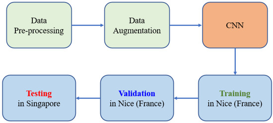
Figure 2.
Flowchart of the methodology.
3.2. Data Processing
With SRTM having a 30 m horizontal resolution, the reference DEM with 1 m, and Sentinel-2 with 10–60 m, all input and output layers were standardized to a 10 m resolution using the nearest neighbor approach [47]. Additionally, ground truth elevations were referenced in the Earth Gravitational Model 96 (EGM96) geoid heights [48], and therefore, all elevations were converted to geoid height.
All input data were processed and divided into training, validation, and testing datasets. The areas covered by these datasets are shown in Figure 3. The training dataset was over an area of 12 km2 in Nice (the box with blue comb pattern in Figure 3a); the validation dataset was over an area of 5.2 km2 (the box with red comb pattern in Figure 3a); and the testing dataset was an area of 2.6 × 4.8 km in the Orchard Road area of Singapore (shown in Figure 3b). The training and validation sites are mainly urbanized with buildings, and the elevation profiles vary from 0 m to 200 m. The average building height is 19.1 m (maximum 60.8 m), and buildings occupy 34% of the total area. Similarly, the test site in Orchard Road, Singapore is also a dense urban area with many high-rise buildings with elevations ranging from 0 m to 150 m. The average building height is 24.5 m (maximum 130 m), and buildings occupy 36% of the total area.
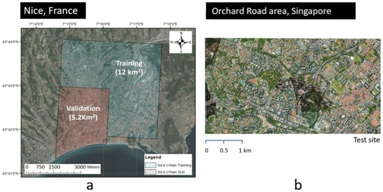
Figure 3.
The images of datasets that were used for: (a) training and validation sites, (b) testing site.
3.3. CNN Configuration
The MATLAB Deep Learning Toolbox was applied in this study for DEM enhancement. We used U-Net structure to design the CNN model. In U-Net structure, the initial series of convolutional layers are interspersed with max pooling layers, successively decreasing the resolution of the input image. These layers are followed by a series of convolutional layers interspersed with up-sampling operators, successively increasing the resolution of the input image. Combining these two series paths forms a U-shaped graph. The CNN model was trained by multi-channel input data. Each input channel represented a feature at 10 m spatial resolution. The datasets mentioned above were processed and divided into training, validation, and testing sets.
CNNs are widely applied in deep learning. CNNs are capable of capturing the spatial and temporal dependencies in an image via application of appropriate convolutional filters. In other words, they learn not only from the input features available for a given pixel or grid cell, but also from those of its neighbors, accounting for potential spatial relationships in that neighborhood. The CNN was widely used in image classification and segmentation tasks, but limited cases of its application are in topography data improvement.
We developed our CNN model based on U-Net architecture, which was fundamentally applied for bio-medical imaging by O. Ronneberger et al. [38]. The architecture consisted of an encoder and a decoder. The encoder was to deal with covenant layers and extract the factors in an image. The decoder used transposed convolution to allow localization. It should be noted that the CNN model developed in this research does not include fully convolutional layers as commonly used in segmentation. Additional convolutional layers were added to allow the model to generate intact images (rather than single values or labels). The structure of the CNN model used in this paper is shown in Figure 4.
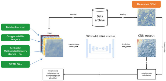
Figure 4.
The structure of the CNN model.
There are 13 input features that are used for the CNN model presented in this paper. The input features include: SRTM_DEM, 8 bands of Sentinel-2 multispectral imagery, 3 bands of RGB from Google satellite imagery, and building footprints from OpenStreetMap Buildings. The target data were high-resolution reference DEM data (or ground truth DEM). All the input features and target data were standardized to a 10 m resolution through the nearest neighbor sampling method.
We used the MATLAB built-in function randomPatchExtractionDatastore to extract randomly positioned patches in size 32 × 32 grid cells from 13 input features and target data. Moreover, to populate the training data, we also used MATLAB built-in function imageDataAugmenter to apply random reflection in the left–right direction and 90 degree rotation to the input features and target data.
The CNN model was trained, and hyper-parameter tuning (parameters are manually defined when the model is initialized) was performed to ensure the convergence and good performance of the model. The optimal hyper-parameters after tuning are shown in Table 1.

Table 1.
Hyper-parameters used by CNN model.
With the choice of the optimal hyper-parameters, the CNN model used 13 input features mentioned above and was trained against reference DEM data (target data). There are two different approaches for the CNN model considered in this study: iConvDEM-1 and iConvDEM-2. The flowchart of data usage for iConvDEM-1 and iConvDEM-2 is shown in Figure 5.
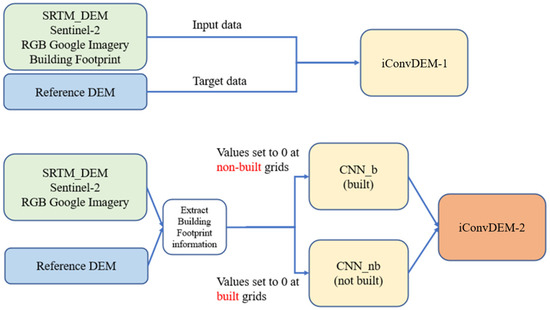
Figure 5.
The flowchart of data usage for iConvDEM-1 and iConvDEM-2.
In the first approach, iConvDEM-1, the CNN model was trained against target data with no special treatments for building and non-building features; they were all in one input dataset. The performance of the iConvDEM-1 model was promising, but the improvement for SRTM DEM was not much different from that of Kim et al. [5] using the ANN.
The second approach, iConvDEM-2, was developed based on the analysis of SRTM data versus reference DEM data. For the available data used in the scope of this work, SRTM data underestimated over building grid cells and overestimated over non-building grid cells. This implied that one CNN model may not perform well for both building and non-building areas. This was a significant finding in the application of the machine learning approach for improving SRTM data over dense urban areas. Kim et al. [5] reached a similar finding as well. In order to address this issue, we proposed a new CNN model (referred to henceforth as iConvDEM-2 in this paper). The iConvDEM-2 model consisted of two separate CNN training processes, one just with buildings (CNN_b) and the other without buildings (CNN_nb). The performance of iConvDEM-2 over dense urban areas, shown later in Section 4, is much better than that of iConvDEM-1.
3.4. Evaluation Methods
The DEM enhancement evaluation was undertaken through visual clarifying, scatterplots, and three statistical measures, the error (E), the absolute error (AE) and root mean square error (RMSE) [5,25,49].
The error (or bias) and absolute error calculate the magnitude of errors between the surveyed (yi) and simulated (Yi) elevations at all grid points (N) in the DEMs (Equation (1)).
The mean absolute error is the average of all grid points in the study area, which is calculated as in Equation (2).
RMSE is the square root of the average of squared differences between surveyed (yi) and simulated (Yi) elevations at all grid points (N) in the DEMs (Equation (3)). The RMSE is the standard way to compute the degree of accuracy between a set of estimates and the actual values [50].
In a set of estimates, both MAE and RMSE are applied to investigate the differences in any errors. If the values are close to zero, then the performance of the estimation output is considered good.
4. Results and Discussions
4.1. Preliminary Results
In this section, we evaluated the performance of different approaches for the validation site in Nice, France (within the box with blue comb pattern in Figure 3a). The two approaches using CNN were iConvDEM-1 and iConvDEM-2 (presented in Section 3.3), which were used to compare against the standard ANN presented in Kim et al. [5] (referred to as ANN [1] in this study).
We first introduced the comparison between the original SRTM DEM and reference DEM. The elevation maps of SRTM DEM and reference DEM data at the validation site in Nice are shown in Figure 6a and Figure 6b, respectively. Figure 6c shows the absolute error between the reference DEM and SRTM DEM. The mean absolute error between reference DEM and SRTM DEM was about 6.8 m, and most of the grid cells with high value absolute error were located at the right side of the map where the area is mainly urbanized with buildings.
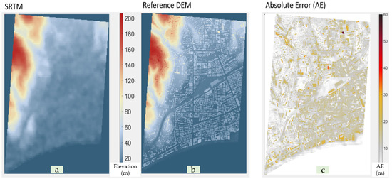
Figure 6.
Elevation map at validation site of: (a) SRTM-DEM, (b) reference DEM and (c) absolute error between reference DEM and SRTM DEM.
We then analyzed the accuracy of DEM generated by the proposed schemes. Figure 7 shows the spatial distribution for absolute error versus reference DEM of SRTM DEM, ANN [1], iConvDEM-1, and iConvDEM-2. Figure 7a shows the highest values of absolute error (majority of grid cells are in dark yellow color, corresponding with absolute error around 10–20 m). Figure 7b,c show more white and light-gray color grid cells (representing absolute error below 10 m) in comparison with the display in Figure 7a. This means that there was a significant improvement for SRTM data using the iConvDEM-1 and ANN [1] model. However, iConvDEM-2 showed the best performance of all by presenting a majority of white and light-gray color grid cells (representing absolute error below 10 m) in its absolute error plot against reference DEM data (Figure 7d).
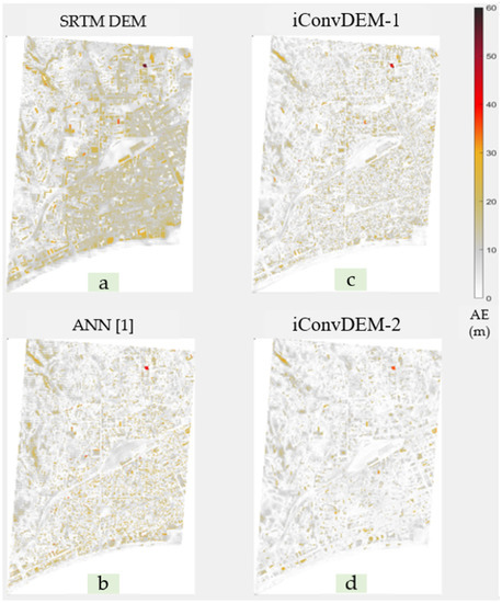
Figure 7.
Absolute error, versus reference DEM, of: (a) SRTM DEM, (b) ANN [1], (c) iConvDEM-1 and (d) iConvDEM-2.
The numerical values of absolute errors and root mean square error (the lower, the better) for all approaches versus reference DEM are shown in Table 2. We can see that iConvDEM-2 outperformed other models with the lowest values of error in all categories. This indicates that the DEM generated by iConvDEM-2 was in best agreement with the reference DEM data.

Table 2.
Performance of all approaches versus reference DEM data.
Figure 8 shows the cumulative distribution of absolute error (AE) values of all approaches versus reference DEM data. The x-axis represents values (in m) of AE while the y-axis shows accumulative distribution of AE values at all grid cells (from 0% to 100%). We see that only about 70% of grid cells of SRTM_DEM (black curve) had AE values lower than 10 m. ANN [1] (blue curve) and iConvDEM-1 (pink curve) showed promising improvement with around 90% of grid cells having AE values lower than 10 m and about 70% of grid cells having AE values lower than 5 m. iConvDEM-2 showed the best performance with 95% of grid cells having AE values lower than 10 m and about 80% of grid cells having AE values lower than 5 m.
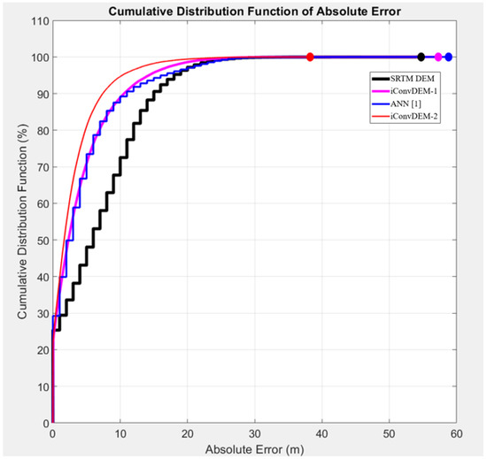
Figure 8.
Cumulative distribution of absolute error values of all approaches versus reference DEM data.
As iConvDEM-2 outperforms other approaches, the remaining Section 4.2 and Section 4.3 assess the performance of iConvDEM-2 when applied to a validation site in Nice and a test site in Singapore.
4.2. Validation of iConvDEM-2 in Nice, France
The comparisons of elevation maps among SRTM DEM, reference DEM and iConvDEM-2 are shown in Figure A1 (in Appendix A). The elevation map generated by iConvDEM-2 showed much clearer land shapes of buildings and roads when compared with SRTM DEM. Moreover, the RMSE (versus reference DEM) of iConvDEM-2 was reduced significantly, to 4.8 m from 9.2 m of SRTM DEM (a 48% reduction).
For better visualization, we selected a zoomed-in site (or sub-area) covering a 1.4 km × 1.4 km area at the center of the validation site in Nice, France. The sub-area is seen bounded by the red box inside satellite imagery in Figure A1. The comparison of elevation maps between SRTM DEM, reference DEM and iConvDEM-2 over the sub-area is shown in Figure 9.
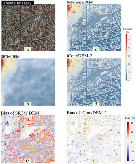
Figure 9.
Plots of sub-area within the validation site in Nice from (a) Satellite image, (b) reference DEM, (c) SRTM DEM, (d) iConvDEM-2, (e) bias of SRTM DEM and (f) bias of iConvDEM-2.
Figure 9a is a satellite image of the validation area showing the land shapes; Figure 9b–d are the elevation maps of SRTM DEM, reference DEM and iConvDEM-2, respectively. The reference DEM is at the highest available quality and shows clear shapes of buildings and roads. The iConvDEM-2 agrees well with the reference DEM and thus shows significant improvements when compared with SRTM DEM.
We computed the bias against the reference DEM to evaluate the quality of SRTM and iConvDEM. The bias maps in Figure 9e were constructed by simply calculating the differences (errors) between reference DEM and SRTM DEM. Similarly, Figure 9f shows the differences between reference DEM and iConvDEM-2. We could see that iConvDEM-2 showed far less bias (error) than SRTM DEM. In Figure 9f, the bias values are mostly within −10 m to 10 m. The light blue color implies overestimation of elevation by iConvDEM-2 over non-building land areas, and the light yellow color implies underestimation of elevation by iConvDEM-2 over building areas. We also observed a similar behavior (overestimation over non-building land areas and underestimation over building areas) with SRTM DEM. However, the light red color and dark blue color in Figure 9e demonstrate much higher bias with SRTM DEM (within −30 m to 30 m). The elevation data improvement with iConvDEM-2 over SRTM DEM is further demonstrated in Figure 10.
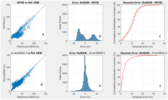
Figure 10.
Statistical analysis for sub-area within validation site in Nice, versus reference DEM, of: (a) elevations of SRTM DEM, (b) errors of SRTM DEM, (c) absolute errors of SRTM DEM, (d) elevations of iConvDEM-2, (e) errors of iConvDEM-2 and (f) absolute errors of iConvDEM-2.
Figure 10a–c show statistical analysis for SRTM DEM versus reference DEM; while Figure 10d–f show statistical analysis for iConvDEM-2 versus reference DEM. The scatter plots of elevation values in Figure 10a,d show that iConvDEM-2 was improved significantly and compared well with the reference DEM, especially at high elevation values (>50 m). Figure 10b,e show the frequency error distribution of SRTM DEM and iConvDEM-2. In Figure 10b, double peaks around −15 m and 15 m implied that the majority of data points (pixels) of SRTM DEM had an error of 15 m in comparison with the reference DEM. In Figure 10e, a single peak close to zero shows that iConvDEM-2 is very close to reference DEM. Moreover, the large bias of SRTM DEM is demonstrated in Figure 10c, where the cumulative distribution function of absolute error between reference DEM and SRTM DEM is shown. Only 20% of the data points in SRTM DEM had absolute error of less than 5 m, while another 60% of data points had absolute error within the range 5–15 m. The rest of the data points (20%) were at more than 15 m in absolute error. On the other hand, more than 80% of the data points in iConvDEM-2 had absolute error of less than 5 m, which is shown in Figure 10f.
4.3. Testing of iConvDEM-2 in Orchard Road Area, Singapore
To test the performance of iConvDEM-2, which was trained and validated in Nice, we selected a dense urban area as the test site. The selected test site was in a dense urban Orchard Road area in Singapore (Figure 3b). The quality of input SRTM DEM data and output data generated by iConvDEM-2 was compared against that of a reference DEM provided by the Singapore’s Building and Construction Authority (BCA). The satellite image of the test site together with elevation maps of SRTM DEM, reference DEM and iConvDEM-2 are shown in Figure A2 (in Appendix A). The elevation generated by iConvDEM-2 matched the reference DEM more than the SRTM DEM. The RMSE (versus reference DEM) of iConvDEM-2 was reduced significantly, to 12.8 m from 18.5 m of SRTM DEM (a 30.8% reduction).
Similarly to the validation process, we selected a zoomed-in site (or sub-area) covering a 1.4 × 1.4 km area within the test site in the Orchard Road area for better visualization. The sub-area is seen bounded by the red box inside the satellite imagery in Figure A2a. The comparison of elevation maps between SRTM DEM, reference DEM and iConvDEM-2 over the sub-area is shown in Figure 11.
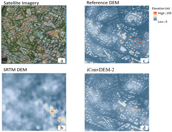
Figure 11.
Plots at sub-area within the test site in Orchard Road area of: (a) satellite image, (b) reference DEM, (c) SRTM DEM and (d) iConvDEM-2.
Figure 11a is a satellite image of the test area delineating the land shapes; Figure 11b–d are the elevation maps of SRTM DEM, reference DEM and iConvDEM-2, respectively. The iConvDEM-2 again shows clearer shapes of buildings and roads than does the original SRTM DEM. In addition, building heights generated by iConvDEM-2 matched well with the reference DEM and clearly showed better quality than SRTM DEM. Significant improvement of iConvDEM-2 is also reflected in the analysis in Figure 12.
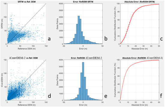
Figure 12.
Statistical analysis of sub-area within the test site in Orchard Road, Singapore, versus reference DEM, of: (a) elevations of SRTM DEM, (b) errors of SRTM DEM, (c) absolute errors of SRTM DEM, (d) elevations of iConvDEM-2, (e) errors of iConvDEM-2 and (f) absolute errors of iConvDEM-2.
Figure 12a–c show statistical analysis for SRTM DEM versus reference DEM, while Figure 12d–f show statistical analysis for iConvDEM-2 versus reference DEM. Comparing the scatter plots of elevation values in Figure 12a,d, iConvDEM-2 shows better agreement with reference DEM, especially at high elevation values around 50 m. Figure 12b,e show the frequency error distribution of SRTM DEM and iConvDEM-2. In Figure 12b, the peak is around −15 m, implying that SRTM DEM shows overestimation, and the majority of the data points (pixels) of SRTM DEM have an error of 15 m in comparison with those of the reference DEM. In Figure 12e, a single peak close to zero shows that iConvDEM-2 agreed quite well with reference DEM. Moreover, the large bias of SRTM DEM is demonstrated in Figure 12c, where the cumulative distribution function of absolute error between reference DEM and SRTM DEM is shown. Only 40% of the data points of SRTM DEM had an absolute error of less than 10 m, while 20% of the data points had an absolute error higher than 20 m. On the other hand, more than 80% of the data points of iConvDEM-2 had an absolute error of less than 10 m, which is shown in Figure 12f. However, the fact that about 10% of the data points had absolute error higher than 20 m implies some weakness in the application of iConvDEM-2 for the test site in the Orchard Road area of Singapore. This can be attributed to the complexity of building profiles in the Orchard Road area. There are many high buildings in the Orchard Road area, and the maximum height of the buildings is more than 100 m (compared with the Nice area used to train iConvDEM-2, with less building density and a maximum building height of 60.8 m).
4.4. Application of iConvDEM-2 in Other Areas with AW3D Input Data
In this section, we would like to show the applicability of the proposed CNN method to an urban area in Jakarta, Indonesia. The input DEM was an AW3D at 2.5 m spatial resolution. Other input channels (8 bands of Sentinel-2 multispectral imagery, 3 bands RGB from Google satellite imagery and building footprint from OpenStreetMap Buildings) were also prepared for the application site.
Figure 13a is a satellite image of the validation area showing the land shapes of the dense urban area in Jakarta, Indonesia; Figure 13b,c are the elevation maps of SRTM DEM and iConvDEM-2, respectively. Even though the reference DEM was not available for further evaluation, we could see that the elevation map generated by iConvDEM-2 definitely showed much clearer land shapes of buildings and roads when compared with the original AW3D.
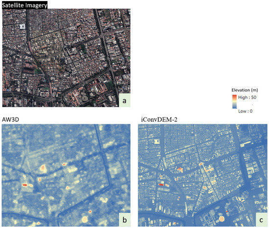
Figure 13.
Plots at application site in Jakarta: (a) Satellite image, (b) SRTM DEM and (c) iConvDEM-2.
5. Conclusions
This paper presented the use of a CNN model to improve SRTM DEM in dense urban cities with different treatments for built and non-built features. The CNN model used a U-Net structure configuration with SRTM DEM, Sentinel 2 multispectral imagery and Google imagery as input channels, while a high-resolution reference DEM was used as target data. To better address the high percentage of buildings within urban cities, the iConvDEM-2 model was introduced with two training processes, one with and one without buildings. By doing so, iConvDEM-2 outperformed the single model that handled both building and non-building features (iConvDEM-1). Moreover, the iConvDEM-2 model also showed better performance when compared to the work using an ANN, shown in Kim et al. [5].
The iConvDEM-2 model was trained in Nice, France and validated at a different site in Nice. The performance of iConvDEM-2 showed significantly better results than that of SRTM DEM. At the validation site in Nice, the RMSE reduction of iConvDEM-2 was about 50% when compared with SRTM DEM, and the visibility (land shapes, buildings, and roads) of iConvDEM-2 was much clearer than that of SRTM DEM. Most of the absolute errors (versus reference DEM) from iConvDEM-2 were below 5 m. This was a significant improvement because the original SRTM DEM had a majority of its absolute error values above 10 m.
The iConvDEM-2 was shown in testing to perform very well when applied to a faraway location (Orchard Road area in Singapore). The RMSE reduction of iConvDEM-2 remained quite impressive at 30%, and its visibility (land shapes, buildings, and roads) was far clearer than that of the original SRTM DEM. Over Singapore’s Orchard Road area, a majority (80%) of the absolute errors (versus reference DEM) of iConvDEM-2 were below 10 m (while the original SRTM DEM had only 40% of absolute errors that fell below 10 m).
The iConvDEM-2 model presented in this paper was proven to enhance the quality of SRTM DEM. In addition, the CNN approach proposed in this study can also be applied to different input DEMs at any spatial resolution, such as AW3D [21] and TanDEM-X [51]. Moreover, the trained CNN model can be applied to any site that has an urbanization profile similar to that of the training site.
Generally, the method can be implemented to improve any satellite DEM data and in any urban city. The work presented in this paper effectively and efficiently obtained a good-quality, high-resolution DEM at low cost. The results of this work have promising potential to be applied over many urban cities, especially in developing countries where high quality DEM data are usually not available or very costly. Good-quality DEMs at high spatial resolutions generated, for example, by the proposed DEM improvement scheme with the CNN model are an indispensable input parameter in flood simulations to assess the impacts of changing climate and sea level rise.
Author Contributions
Conceptualization, N.S.N., D.E.K., Y.J., S.V.R. and S.Y.L.; methodology, N.S.N. and S.Y.L.; software, N.S.N.; validation, N.S.N., D.E.K. and Y.J.; formal analysis, N.S.N. and D.E.K.; investigation, S.Y.L.; resources, S.V.R. and S.Y.L.; data curation, N.S.N., D.E.K. and Y.J.; writing—original draft preparation, N.S.N.; writing—review and editing, S.V.R. and S.Y.L.; visualization, N.S.N. and Y.J.; supervision, S.Y.L.; project administration, S.V.R. and S.Y.L.; funding acquisition, D.E.K. and S.Y.L. All authors have read and agreed to the published version of the manuscript.
Funding
This research was funded by the National Research Foundation, Singapore through the AI Singapore Programme (AISG Award No: AISG-100E/GC/RP/RPKS-2019-045) and DHI Water & Environment (Singapore).
Data Availability Statement
Not applicable.
Acknowledgments
This research was supported by (1) the National Research Foundation, Singapore through the AI Singapore Programme (AISG Award No: AISG-100E/GC/RP/RPKS-2019-045) and (2) DHI Water & Environment (Singapore). The authors thank the (1) Métropole Nice Côte d’Azur, France and (2) Building and Construction Authority of Singapore for providing the DEM data.
Conflicts of Interest
The authors declare no conflict of interest.
Appendix A
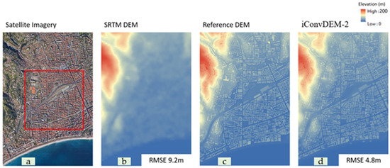
Figure A1.
Plots at the validation site in Nice of: (a) satellite image, (b) SRTM DEM, (c) reference DEM and (d) iConvDEM-2.
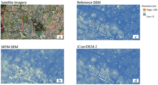
Figure A2.
Plots at the testing site in the Orchard Road area (Singapore) of: (a) satellite image, (b) SRTM DEM, (c) reference DEM and (d) iConvDEM-2.
References
- Hawker, L.; Bates, P.; Neal, J.; Rougier, J. Perspectives on Digital Elevation Model (DEM) Simulation for Flood Modeling in the Absence of a High-Accuracy Open Access Global DEM. Front. Earth Sci. 2018, 6, 233. [Google Scholar] [CrossRef] [Green Version]
- Moudrý, V.; Lecours, V.; Gdulová, K.; Gábor, L.; Moudrá, L.; Kropácek, J.; Wild, J. On the use of global DEMs in ecological modelling and the accuracy of new bare-earth DEMs. Ecol. Model. 2018, 383, 3–9. [Google Scholar] [CrossRef]
- Wang, D.; Kääb, A. Modeling glacier elevation change from DEM time series. Remote Sens. 2015, 7, 10117–10142. [Google Scholar] [CrossRef] [Green Version]
- Zhang, W.; Montgomery, D.R. Digital elevation model grid size, landscape representation, and hydrologic simulations. Water Resour. Res. 1994, 30, 1019–1028. [Google Scholar] [CrossRef]
- Kim, D.E.; Liong, S.Y.; Gourbesville, P.; Andres, L.; Liu, J. Simple-Yet-Effective SRTM DEM Improvement Scheme for Dense Urban Cities Using ANN and Remote Sensing Data: Application to Flood Modeling. Water 2020, 12, 816. [Google Scholar] [CrossRef] [Green Version]
- Kim, D.E.; Sun, Y.; Wendi, D.; Jiang, Z.; Liong, S.Y.; Gourbesville, P. Flood modelling framework for Kuching City, Malaysia: Overcoming the lack of data. In Advances in Hydroinformatics; Springer: Berlin, Germany; Heidelberg, Germany, 2018; pp. 559–568. [Google Scholar]
- Kim, D.E.; Gourbesville, P.; Liong, S.Y. Overcoming data scarcity in flood hazard assessment using remote sensing and artificial neural network. Smart Water 2019, 4, 2. [Google Scholar] [CrossRef]
- Kim, D.E.; Liu, J.; Liong, S.Y.; Gourbesville, P.; Strunz, G. Satellite DEM Improvement Using Multispectral Imagery and an Artificial Neural Network. Water 2021, 13, 1551. [Google Scholar] [CrossRef]
- Meadows, M.; Wilson, M. A Comparison of Machine Learning Approaches to Improve Free Topography Data for Flood Modelling. Remote Sens. 2021, 13, 275. [Google Scholar] [CrossRef]
- Sanders, B.F. Evaluation of on-line DEMs for flood inundation modeling. Adv. Water Resour. 2007, 30, 1831–1843. [Google Scholar] [CrossRef]
- Wilson, M.D.; Bates, P.; Alsdorf, D.; Forsberg, B.; Horritt, M.; Melack, J.; Frappart, F.; Famiglietti, J. Modeling large-scale inundation of Amazonian seasonally flooded wetlands. Geophys. Res. Lett. 2007, 34, 4–9. [Google Scholar] [CrossRef] [Green Version]
- Zhang, K.; Gann, D.; Ross, M.; Robertson, Q.; Sarmiento, J.; Santana, S.; Rhome, J.; Fritz, C. Accuracy assessment of ASTER, SRTM, ALOS and TDX DEMs for Hispaniola and implications for mapping vulnerability to coastal flooding. Remote Sens. Environ. 2019, 225, 290–306. [Google Scholar] [CrossRef]
- Nardi, F.; Annis, A.; Baldassarre, G.D.; Vivoni, E.R.; Grimaldi, S. GFPLAIN250m, a global high-resolution dataset of earth’s floodplains. Sci. Data 2019, 6, 180309. [Google Scholar] [CrossRef] [PubMed]
- Annis, A.; Nardi, F.; Petroselli, A.; Apollonio, C.; Arcangeletti, E.; Tauro, F.; Belli, C.; Bianconi, R.; Grimaldi, S. UAV-DEMs for Small-Scale Flood Hazard Mapping. Water 2020, 12, 1717. [Google Scholar] [CrossRef]
- He, Y.; Song, Z.; Liu, Z. Updating highway asset inventory using airborne LiDAR. Measurement 2017, 104, 132–141. [Google Scholar] [CrossRef]
- Mesa-Mingorance, J.L.; Ariza-López, F.J. Accuracy Assessment of Digital Elevation Models (DEMs): A Critical Review of Practices of the Past Three Decades. Remote Sens. 2020, 12, 1630. [Google Scholar] [CrossRef]
- Polidori, L.; El Hage, M. Digital Elevation Model Quality Assessment Methods: A Critical Review. Remote Sens. 2020, 12, 3522. [Google Scholar] [CrossRef]
- Simpson, A.L.; Balog, S.; Moller, D.K.; Strauss, B.H.; Saito, K. An urgent case for higher resolution digital elevation models in the world’s poorest and most vulnerable countries. Front. Earth Sci. 2015, 3, 50. [Google Scholar] [CrossRef] [Green Version]
- Farr, T.G.; Rosen, P.A.; Caro, E.; Crippen, R.; Duren, R.; Hensley, S.; Kobrick, M.; Paller, M.; Rodriguez, E.; Roth, L. The shuttle radar topography mission. Rev. Geophys. 2007, 45, RG2004. [Google Scholar] [CrossRef] [Green Version]
- Tachikawa, T.; Kaku, M.; Iwasaki, A.; Gesch, D.B.; Oimoen, M.J.; Zhang, Z.; Danielson, J.J.; Krieger, T.; Curtis, B.; Haase, J. ASTER Global Digital Elevation Model Version 2-Summary of Validation Results; NASA: Mountain View, CA, USA, 2011.
- Florinsky, I.; Skrypitsyna, T.; Luschikova, O. Comparative accuracy of the AW3D30 DSM, ASTER GDEM, and SRTM1 DEM: A case study on the Zaoksky testing ground, Central European Russia. Remote Sens. Lett. 2018, 9, 706–714. [Google Scholar] [CrossRef]
- Yan, K.; Di Baldassarre, G.; Solomatine, D.P. Exploring the potential of SRTM topographic data for flood inundation modelling under uncertainty. J. Hydroinform. 2013, 15, 849–861. [Google Scholar] [CrossRef]
- Domeneghetti, A. On the use of SRTM and altimetry data for flood modeling in data-sparse regions. Water Resour. Res. 2016, 52, 2901–2918. [Google Scholar] [CrossRef] [Green Version]
- Boulton, S.J.; Stokes, M. Which DEM is best for analyzing fluvial landscape development in mountainous terrains? Geomorphology 2018, 310, 168–187. [Google Scholar] [CrossRef]
- Wendi, D.; Liong, S.Y.; Sun, Y.; Doan, C.D. An innovative approach to improve SRTM DEM using multispectral imagery and artificial neural network. J. Adv. Modeling Earth Syst. 2016, 8, 691–702. [Google Scholar] [CrossRef] [Green Version]
- Rodriguez, E.; Morris, C.S.; Belz, J.E. A global assessment of the SRTM performance. Photogramm. Eng. Remote Sens. 2006, 72, 249–260. [Google Scholar] [CrossRef] [Green Version]
- Jordan, R.L.; Caro, E.R.; Kim, Y.; Kobrick, M.; Shen, Y.; Stuhr, F.V.; Werner, M.U. Shuttle Radar Topography Mapper (SRTM). In Proceedings of the SPIE 2958, Microwave Sensing and Synthetic Aperture Radar, Taormina, Italy, 17 December 1996. [Google Scholar] [CrossRef]
- Maire, C.; Datcu, M.; Audenino, P. SAR DEM filtering by mean of Bayesian and multi-scale, nonstationary methods. In Proceedings of the IGARSS 2003—2003 IEEE International Geoscience and Remote Sensing Symposium, Toulouse, France, 21–25 July 2003; Volume 6, pp. 3916–3918. [Google Scholar]
- Stevenson, J.A.; Sun, X.; Mitchell, N.C. Despeckling SRTM and other topographic data with a denoising algorithm. Geomorphology 2010, 114, 238–252. [Google Scholar] [CrossRef]
- Ettritch, G.; Hardy, A.; Bojang, L.; Cross, D.; Bunting, P.; Brewer, P. Enhancing digital elevation models for hydraulic modelling using flood frequency detection. Remote Sens. Environ. 2018, 217, 506–522. [Google Scholar] [CrossRef]
- Kulp, S.A.; Strauss, B.H. CoastalDEM: A global coastal digital elevation model improved from SRTM using a neural network. Remote Sens. Environ. 2018, 206, 231–239. [Google Scholar] [CrossRef]
- Yamazaki, D.; Ikeshima, D.; Tawatari, R.; Yamaguchi, T.; O’Loughlin, F.; Neal, J.C.; Sampson, C.C.; Kanae, S.; Bates, P.D. A high-accuracy map of global terrain elevations. Geophys. Res. Lett. 2017, 44, 5844–5853. [Google Scholar] [CrossRef] [Green Version]
- Bhardwaj, A.; Jain, K.; Chatterjee, R.S. Generation of high-quality digital elevation models by assimilation of remote sensing-based DEMs. J. Appl. Remote Sens. 2019, 13, 044502. [Google Scholar] [CrossRef]
- Ajibola, I.I.; Mansor, S.; Pradhan, B.; Shafri, H.Z.M. Fusion of UAV-based DEMs for vertical component accuracy improvement. Measurement 2019, 147, 106795. [Google Scholar] [CrossRef]
- Muhadi, N.A.; Mohd Kassim, M.S.; Abdullah, A.F. Improvement of Digital Elevation Model (DEM) using data fusion technique for oil palm replanting phase. Int. J. Image Data Fusion 2019, 10, 232–243. [Google Scholar] [CrossRef]
- Lary, D.J.; Zewdie, G.K.; Liu, X.; Wu, D.; Levetin, E.; Allee, R.J.; Malakar, N.; Walker, A.; Mussa, H.; Mannino, A.; et al. Machine Learning Applications for Earth Observation. In Earth Observation Open Science and Innovation; ISSI Scientific Report Series 15; Mathieu, P., Aubrecht, C., Eds.; International Space Science Institute (ISSI): Bern, Switzerland, 2018; ISBN 9783319656328. [Google Scholar]
- Global Facility for Disaster Reduction and Revovery. Machine Learning for Disaster Risk Management; Global Facility for Disaster Risk Reduction and Recovery (GFDRR): Washington, DC, USA, 2018. [Google Scholar]
- Ronneberger, O.; Fischer, P.; Brox, T. U-net: Convolutional networks for biomedical image segmentation. Lect. Notes Comput. Sci. 2015, 9351, 234–241. [Google Scholar]
- Pyo, J.C.; Duan, H.; Baek, S.; Kim, M.S.; Jeon, T.; Kwon, Y.S.; Lee, H.; Cho, K.H. A convolutional neural network regression for quantifying cyanobacteria using hyperspectral imagery. Remote Sens. Environ. 2019, 233, 111350. [Google Scholar] [CrossRef]
- Long, J.; Shelhamer, E.; Darrell, T. Fully Convolutional Networks for Semantic Segmentation. IEEE Trans. Pattern Anal. Mach. Intell. 2017, 39, 640–651. [Google Scholar]
- Flood, N.; Watson, F.; Collett, L. Using a U-net convolutional neural network to map woody vegetation extent from high resolution satellite imagery across Queensland, Australia. Int. J. Appl. Earth Obs. Geoinf. 2019, 82, 101897. [Google Scholar] [CrossRef]
- U.S. Geological Survey (USGS). USGS EROS Archive—Digital Elevation—Shuttle Radar Topography Mission (SRTM) 1 Arc-Second Global; Earth Resources Observation and Science Center: SiouxFalls, SD, USA, 2018.
- Gatti, A.; Bertolini, A. Sentinel-2 Products Specification Document. 2018. Available online: https://earth.esa.int/documents/247904/685211/Sentinel-2+Products+Specification+Document (accessed on 15 March 2021).
- Drusch, M.; Del Bello, U.; Carlier, S.; Colin, O.; Fernandez, V.; Gascón, F.; Hoersch, B.; Isola, C.; Laberinti, P.; Martimort, P.; et al. Sentinel-2: ESA’s Optical High-Resolution Mission for GMES Operational Services. Remote Sens. Environ. 2012, 120, 25–36. [Google Scholar] [CrossRef]
- Roy, D.P.; Li, J.; Zhang, H.K.; Yan, L.; Huang, H.; Li, Z. Examination of Sentinel-2A multi-spectral instrument (MSI) reflectance anisotropy and the suitability of a general method to normalize MSI reflectance to nadir BRDF adjusted reflectance. Remote Sens. Environ. 2017, 199, 25–38. [Google Scholar] [CrossRef]
- Fan, H.; Zipf, A.; Fu, Q.; Neis, P. Quality assessment for building footprints data on OpenStreetMap. Int. J. Geogr. Inf. Sci. 2014, 28, 700–719. [Google Scholar] [CrossRef]
- Takagi, M. Accuracy of digital elevation model according to spatial resolution. Int. Arch. Photogramm. Remote Sens. 1998, 32, 613–617. [Google Scholar]
- Lemoine, F.; Kenyon, S.; Factor, J.; Trimmer, R.; Pavlis, N.; Chinn, D.; Cox, C.; Klosko, S.; Luthcke, S.; Torrence, M. The Development of the Joint NASA GSFC and the National Imagery and Mapping Agency (NIMA) Geopotential Model EGM96; National Aeronautics and Space Administration, Goddard Space Flight Center: Greenbelt, MD, USA, 1998.
- Szypuła, B. Quality assessment of DEM derived from topographic maps for geomorphometric purposes. Open Geosci. 2019, 11, 843–865. [Google Scholar] [CrossRef]
- Li, Z. On the measure of digital terrain model accuracy. Photogramm. Rec. 1988, 12, 873–877. [Google Scholar] [CrossRef]
- Hajnsek, I.; Busche, T.; Schulze, D.; Buckreub, S.; Moreira, A. TanDEM-X: TanDEM-X Digital Elevation Models Announcement of Opportunity; TD-PD-AO-0033; German Aerospace Center (DLR): Bonn, Germany, 2016. [Google Scholar]
Publisher’s Note: MDPI stays neutral with regard to jurisdictional claims in published maps and institutional affiliations. |
© 2022 by the authors. Licensee MDPI, Basel, Switzerland. This article is an open access article distributed under the terms and conditions of the Creative Commons Attribution (CC BY) license (https://creativecommons.org/licenses/by/4.0/).