Abstract
The study investigates the safe haven properties and sustainability of the top five cryptocurrencies (Bitcoin, Ethereum, Dash, Monero, and Ripple) and gold for BRICS stock markets during the COVID-19 crisis period from 31 January 2020 to 17 September 2020 in comparison to the precrisis period from 1 January 2016 to 30 January 2020, in a nonlinear and asymmetric framework using Nonlinear Autoregressive Distributed Lag (NARDL) methodology. Our results show that the relationship dynamics of stock market and cryptocurrency returns both in the short and long run are changing during the COVID-19 crisis period, which justifies our study using the nonlinear and asymmetric model. As far as a sustainable safe haven is concerned, Dash and Ripple are found to be a safe haven for all the five markets before the pandemic. However, all five cryptocurrencies are found to be a safe haven for three emerging markets, such as Brazil, China, and Russia, during the financial crisis. In a comparative framework, gold is found to be a suitable safe haven only for Brazil and Russia. The results have implications for index fund managers of BRICS markets to include Dash and Ripple in their portfolio as safe haven assets to protect its value during a stock market crisis.
1. Introduction
Ever since the evolution of Bitcoin, as a medium exchange to investment assets and finally as a commodity, recently researchers are fascinated towards studying the safe haven potential of cryptocurrencies in general, and Bitcoin in particular, with respect to the decline in the stock market. It has been seen that investors prefer non-sovereign, non-regulated, and non-political assets during the European crisis in 2010–2013 and the banking crisis of Cyprus in 2012–2013, wherein Bitcoin not only remained unaffected but also thrived (Kristoufek 2015; Luther and Salter 2017).
The recent economic and financial developments related to the crypto market in general and Bitcoin in particular, such as the introduction of Bitcoin futures by CBOE, offering of funds linked to Bitcoin by investment bankers, and heterogeneous regulatory/legal measures (e.g., adoption of digital friendly rules by Japan) across the developed and developing countries, led to shifting of the focus towards the safe haven potential of the cryptocurrencies. Further, recent attention has been shifted towards crypto instruments because it has been seen that speculative behaviour of investors in gold led to the destruction of its hedging properties in US and European markets, particularly after 2013 (Klein 2017). What is expected from a safe haven asset by the portfolio and risk managers during a COVID-19-like stock market crisis characterised by huge volatility1 is that the asset should be able to reduce risk and increase the benefit of diversification.
The current COVID-19-led worldwide financial crisis is actually a real testing time for cryptocurrencies of their safe heaven properties since their inception. Crypto assets in order to be safe haven assets must be negatively correlated or uncorrelated with equity indices in the COVID-19 stock market crisis (Baur and Lucey 2010). Wang et al. (2019b) found that crypto assets are not suitable safe havens for BRICS stock markets using a DCC GARCH framework. The safe haven is tested using dummies for extreme negative market movements. They found that a safe haven is pronounced in the case of a developed, larger market capitalisation and a higher liquid market.
In this study, we have taken a divergent stand from Wang et al. (2019b) and investigated the safe haven property of five crypto assets and gold for BRICS markets. Although safe haven attribution is based on no or negative correlation of the safe haven asset with other assets in a time varying framework, it needs to be seen first how this relationship holds in the short and long term as investors have different investment horizons. Second, how does this relationship behave for a negative or positive change in safe haven assets? Thus, in our study, a safe haven means it is both in the short and long run and also for both positive and negative changes in crypto assets. Our contribution to the literature of safe haven assets is the consideration of the nonlinearity and asymmetric effect in the determination of the safe haven properties of cryptocurrencies using the Nonlinear Autoregressive Distributed Lag (NARDL) methodology of Shin et al. (2014). Our focus is on the safe haven properties of the top five cryptocurrencies2 in the context of the top five biggest emerging markets, i.e., Brazil, Russia, India, China, and South Africa (BRICS). The top five crypto assets are based on market capitalisation (such as Bitcoin, Ethereum, Dash, Ripple, and Monero). Further, for comparative analysis purposes, we have also considered gold along with five cryptocurrencies in our study. During this crisis period two notable features are observed. While VIX made an all-time historic high, the price of oil (WTI) collapsed to an historic low. Since both the developments have a bearing on the stock market, the study accounted for the effect of both in the process of investigating the influence of cryptocurrencies on the stock market during this unprecedented COVID-19-led financial crisis.
Our definition of safe haven is based on the definition provided by Baur and Lucey (2010). In addition to that, the strength of the safe haven property is investigated in a nonlinear and asymmetric framework in line with the study of Baur and McDermott (2010). During the crisis, the safe heaven asset is expected to be either uncorrelated or negatively correlated so that there should not be any loss of value in the asset in such times. Taking a safe haven stand based on negative or no relationship between the safe haven asset and other assets is not enough as the economic and financial world is dynamic, which may change the relationship dynamics. Thus, the market participants should understand if at all the safe haven relationship gets disturbed, thereby impacting the safe haven dynamics, what the strength of the impact will be and how long it will take to come back to the status quo. According to Baur and McDermott (2010), the asset is said to be a strong (weak) safe heaven if it is negatively correlated (uncorrelated) with another asset during a crisis. Thus, such a kind of distinction between a strong and weak safe haven would be helpful to the investors in taking an appropriate safe haven position in appropriate cryptocurrency.
Our results show that, in a nonlinear and asymmetric framework, the relationship dynamics both in the short and long run is changing during the crisis period, which justifies our study using a nonlinear and asymmetric model. Further, Dash and Ripple are found to be a safe haven for all five markets. However, for BVSP, SSE, and RTSI, almost all cryptocurrencies are a safe haven during the financial crisis. Finally, gold is found to be a suitable safe haven only for BVSP and RTSI.
Our study contributes to the safe haven literature in the following dimensions. First, the nonlinear (short and long term) and asymmetric (positive and negative changes) safe haven properties of five top cryptocurrencies in terms of market capitalisation and gold are investigated for the top five emerging markets in terms of market size and liquidity. Secondly, ours is the first study to investigate the sustainability of the safe haven relationship in face of short-term impact due to changes in financial and economic conditions. The short-term impact is studied in terms of its strength and duration for unit changes in cryptocurrency prices. Third, the Nonlinear Autoregressive Distributed Lag (NARDL) model is used for the first time to study the safe haven properties of the cryptocurrencies in a nonlinear and asymmetric framework. Furthermore, it is helpful detecting the sustainability of the safe haven relationship. Fourth, unlike studies in the literature where the safe haven is studied using a dummy for the market crisis, ours is the study which is undertaken during the actual crisis period, i.e., the COVID-19 financial crisis. Fifth, we have conducted a comparative study of the safe haven properties between pre- and during the COVID-19 financial crisis.
2. Literature Review
The literature is very scant as far as the safe haven and hedging properties of the crypto assets, mainly Bitcoin, are concerned. The results are not conclusive in the studies by Wang et al. (2019a), Bouri et al. (2017), Kliber et al. (2019), and Ghorbel and Jeribi (2021) based on the conditional correlation estimated using DCC GARCH methodology and based on spillover of return and volatility by Corbet et al. (2018). The safe haven properties of Bitcoin are found to be time and frequency varying (Bouri et al. 2020). In an intraday framework using the ADCC GARCH model, Urquhart and Zhang (2019) found Bitcoin as a safe haven for currencies such as CHF, EUR, and GBP. Studying some features such as volatility and liquidity, Smales (2018) denies the worthiness of Bitcoin as a safe haven asset and its position lies between a currency and a commodity given its finite size and decentralised size of the market. Kajtazi and Moro (2019) studied the consequences of incorporating Bitcoin to the optimum portfolio by focusing on the mean CVaR method. They investigated the inclusion of Bitcoin in three separate geographically established portfolios of US, European, and Chinese assets, based on its risk-effect. They show that the inclusion of Bitcoin in a portfolio increases its performance, but this is due more to the improvement in returns than in the reduction of volatility. The advantage of the addition of Bitcoin is that the increase in the return on the portfolio compensates for the increase in risk. Gajardo et al. (2018) investigate the asymmetry of the cross-correlation between the major currencies and Bitcoin, WTI and Bitcoin, gold and DJIA, using the MF-ADCCA. They found that in any cross-correlation being studied, there is multi-fractality. They also found that asymmetry is present in cross-correlation exponents under the different trends of gold, DJIA, and WTI. In its cross-correlation to WTI, gold, and DJIA, their findings reveal that Bitcoin represents more multi-fractal spectra than the other currencies. Bouri et al. (2018) investigate the nonlinear and asymmetric impact of the aggregate commodity index and gold price on Bitcoin using the NARDL modelling approach. Their results highlight that the Bitcoin price could be predicted based on price information from aggregate commodity and gold. Jareño et al. (2020) analyses the sensitivity of Bitcoin returns to gold returns and other assets, such as S&P500, using the NARDL framework. Findings show that Bitcoin responds asymmetrically to the considered macroeconomic and financial determinants. González et al. (2021) investigated the interdependence between the twelve largest cryptocurrency returns and gold returns. Results show that cryptocurrency returns are more correlated during the COVID-19 crisis and are cointegrated with gold returns in the crisis period. NARDL results show a positive and statistically significant connectedness between them.
In a recent study related to the COVID-19 crisis, Conlon and McGee (2020) refuted the safe haven claim of Bitcoin based on the quantification of downside risk of the portfolio consisting of equity and Bitcoin using VaR and Conditional VaR approaches. Using several copula models, Garcia-Jorcano and Benito Muela (2020) suggested that Bitcoin can be considered as a hedge asset against the US, European, Japanese, and Chinese stock market indices’ movements under normal market conditions. However, under extreme market conditions, Bitcoin changes to become a diversifier asset. The existing literature on the safe-haven property of cryptocurrencies and gold is found to be either confined to developed or developing countries, or even if it is in the context of both, in that case the focus is on Bitcoin only (Dyhrberg 2016; Pal and Mitra 2019; Smales 2018; Urquhart and Zhang 2019). However, only a few authors, such as Wei (2018), Phillip et al. (2018), Corbet et al. (2018), Bouri et al. (2018), Wang et al. (2019b), and Jeribi and Fakhfekh (2021) are found to be studying the safe haven property of other cryptocurrencies. Ghorbel and Jeribi found that Bitcoin and gold were considered as a hedge for the US investors before the coronavirus crisis. However, they argued that, unlike gold, cryptocurrencies were not a safe haven for US investors during the 2020 global crisis.
In the context of G7 countries, while few cases of safe haven properties are observed for Bitcoin, gold emerged as the stronger diversifier in a downward market as evidenced from a traditional regression analysis study by Shahzad et al. (2019). However, in a comparative framework, Bouri et al. (2020) supports the superiority of Bitcoin as a potential diversifier at the tail of the distribution using Wavelet VaR methodology. Corbet et al. (2018), based on measures of connectedness spillover, stated that isolation of Bitcoin from other financial assets was observed, thereby supporting the benefits of diversification opportunity. However, Klein et al. (2018) found that, fundamentally, the properties of gold are different from Bitcoin independently as an asset and also in terms of their linkage with the stock market. It is seen during a stress period in the market that different financial assets, such as gold, silver, and Bitcoin, behave differently with the stock market based on their unconditional correlation, where gold and silver are found to maintain the characteristics of a safe haven asset unlike Bitcoin. Moreover, in terms of portfolio hedging in the extreme down market, unlike gold, Bitcoin does not show any hedging property.
Our study is related to Wang et al. (2019b) who found that a safe haven is pronounced in the case of developed, larger market capitalisation and a higher liquid market and no cryptocurrency is found to be a safe haven for the emerging market countries such as BRICS markets. Taking the cue from Wang et al. (2019b), our study focuses on developing markets, i.e., BRICS markets and the top five cryptocurrencies in terms of market size and liquidity (Corbet et al. 2019). Lahiani and Jlassi (2021) investigate the median and tail dependence between cryptocurrency and stock market returns of BRICS and developed countries. They indicated that BSE 30 is the best predictor of cryptocurrencies’ returns. Ghorbel and Jeribi (2021) found that the risks among developed stock markets can be hedged by the world’s biggest cryptocurrency and the yellow metal. They considered Bitcoin as the new gold for these economies. Unlike Bitcoin, the yellow metal can be considered as a hedge for Chinese as well as Indian investors. However, these two assets can be considered as diversifier assets on the other BRICS economies. In addition, their results indicated that Dash and Monero can be considered as diversifier assets for developed stock markets.
Further, although a safe haven is attributed based on no or negative correlation of the safe haven asset with other assets in a time varying framework, it needs to be checked first whether this relationship holds in the short and long term as investors have different investment horizons. Second, how does this relationship behave for a negative or a positive change in safe haven asset prices?
3. Data and Methodology
3.1. Data
Our sample period consists of pre- and through the COVID-19 financial crisis period. The pre-crisis period ranges from 1 January 2016 to 30 January 20203 and the COVID-19 financial crisis period spans from 31 January 2020 to 17 September 2020 covering the entire period of the crisis. The daily closing price data have been collected from the CoinDesk Price Index for cryptocurrencies (Bitcoin, Dash, Ethereum, Monero, and Ripple) and from DataStream for gold and stock indices of BRICS countries (such as BVSP of Brazil, RTSI of Russia, BSE Sensex 30 of India, SSE of China, and JSE 40 of South Africa).
During this period, all the cryptos except Bitcoin were stable and the price of Bitcoin fell in sync with the world stock markets, which justifies our study for studying the impact of other cryptocurrencies. The correlation heterogeneity between crypto and stock was also observed across the cryptos.
As evidenced from the mean return of the pre-COVID-19 period presented in the upper panel of Table 1, all five cryptocurrencies are outperforming all the five emerging stock market returns. During the COVID-19 period also, except for Dash, cryptocurrencies are outperforming the emerging equity markets. As far as risk measured in terms of standard deviation is concerned, the cryptocurrencies are observed to be riskier than the equity market in the pre-COVID-19 period. However, in the COVID-19 crisis period, while the risk of equity doubled, the cryptocurrencies are found to be stable. This stability of cryptocurrencies in the COVID-19 crisis could be an opportunity for a safe haven, thus justifying our study during the crisis period. The returns of both equity and cryptocurrencies become more negatively skewed and more jumps are observed as the value of kurtosis increased in the COVID-19 crisis period relative to the pre-COVID-19 period. Gold in both the periods looks stable in terms of return and risk. WTI became more volatile in the crisis period with an average negative return, which was positive in the pre-crisis period. The level of volatility in the equity market has increased during the crisis period in comparison to the pre-crisis period as indicated by VIX. All the return series are non-normal as the Jarque-Bera test highly rejects the null of normality, thus justifying the application of the NARDL model, which considers that nonlinearity is due to short- and long-run effects and also due to positive and negative changes. Further, Maiti et al. (2020) mentioned about the nonlinearity of the daily return of Tether cryptocurrency. The relationship between these two markets is expected not to be linear because while the crypto markets are unregulated, the stock markets across the world are regulated. Further, while the stock markets are related to economic fundamentals, the crypto markets are not.

Table 1.
Stochastic properties of return series dynamics.
The pre-crisis and during crisis period correlation between the five cryptocurrencies, gold, BRICS stock indices, VIX, and WTI are presented in Table 2. There was no correlation found between cryptocurrencies and stock markets in the pre-crisis period. However, during the crisis period, the relationship between all five cryptocurrencies and five stock indices becomes significantly positive. The degree of relationship is high (low) with BVSP (SSE). Thus, this positive relationship rejects any kind of possible safe haven opportunity for cryptocurrencies. However, this relationship is linear and ignores short- and long-term nonlinearity and also the nonlinearity due to positive and negative changes of cryptocurrencies’ prices. Our study estimates the relationship dynamics between cryptocurrencies and stock indices with due consideration to aforementioned nonlinearity.

Table 2.
Correlation dynamics between five crypto assets and BRICS stock indices, gold, VIX, and WTI in pre- and during the COVID-19 crisis period.
To investigate the order of integration of price series, and due to the presence of a turning point in the price dynamics, we ran the breakpoint unit root test (Perron 1989) that allows for one structural break in the data. Results in Table 3 highlight a different order of integration of the cryptocurrencies, stock indices, VIX, WTI, and gold in pre- and during the crisis period. It is a mix of I(1) and I(0) series, leading us to choose the ARDL-type models to investigate the safe haven property of cryptocurrencies and gold while accommodating for the important role of VIX and oil prices. The ARDL-type models were introduced in the econometric literature to investigate the relationship between I(1) and I(0) series by Pesaran et al. (2001).

Table 3.
Breakpoint unit root test.
We further investigated the cointegration relationship between the system of variables (stock market, crypto, WTI, VIX) by performing the Johansen (1992) cointegration test. Results in Table 4 reveal the existence of at least one cointegration relationship among variables in each quadruple, which supports the use of ARDL-type models.

Table 4.
Results of the Johansen cointegration test.
3.2. Methodology
Following the arguments in Section 2, we adopted the NARDL model of Shin et al. (2014) for the following four reasons. First, unlike competing error correction models which require the considered time series to be I(1), the NARDL allows the consideration of data series that have different integration orders, i.e., mix of I(1) and I(0) series. Second, it allows modelling of the cointegration relation that could exist between the stock market prices and cryptocurrency (gold) prices. Third, linear and nonlinear cointegration could be modelled within this framework. Fourth, the NARDL model is a single-equation model that allows the separation of the respective short- and long-run effects of explanatory variables on the dependent variable. It is worth noting that other cointegration models, such as the vector error correction model, accommodate for the previous property of the NARDL model. However, the number of parameters will increase sharply if more variables are introduced in the system as the VECM model consists of a system of equations, which is not the case for the NARDL model.
Concretely, the linear ARDL has the following form:
The goal in this paper is to investigate the safe haven property of cryptocurrencies and gold during the COVID-19 period while accounting for the effects of VIX and WTI prices. Consequently, in the above model, represents the stock price at time , ’ is the vector of explanatory variables that includes the cryptocurrency price among Bitcoin, Dash, Ethereum, Monero, and Ripple. We also considered the case where gold is used instead of cryptocurrency. denotes the VIX volatility index and refers to oil price. is the error term assumed to be white noise.
Indeed, if cryptocurrency (gold) prices retain or gain values during stock price crashes, they are considered as safe haven assets as they allow investors to maintain the profitability of their portfolios. The symbol Δ denotes price variations. Even though the model in Equation (1) has several advantages over traditional cointegration models, it remains simplistic when the relationships between system variables are nonlinear and/or asymmetric. The recently developed cointegrating NARDL model of Shin et al. (2014) allows us to account for the likelihood of an asymmetric effect of cryptocurrency prices, and VIX and WTI prices on stock prices in the short and long run. Practically, this model decomposes the exogenous variable into its positive and negative partial sums for increases and decreases such as:
Accounting for short- and long-run asymmetries in the model represented in Equation (1) leads to the following functional form of the NARDL model with long- and short-run asymmetries:
The superscripts (+) and (–) in Equation (2) refer to the positive and negative partial sums decomposition as computed above. The long-run asymmetry is captured by and . The short-run asymmetry is captured by and . Consequently, long-run asymmetry is tested using a Wald test of the null , while the short-run asymmetry is tested using a Wald test of the null , for . The ARDL-type models have a double advantage. In fact, they permit us to assess the imminent effect of cryptocurrency returns, and VIX and WTI returns on stock market returns. In addition, they allow the measuring of the long-run reaction of stock index prices to cryptocurrency prices, and VIX and WTI prices. The speed of adjustment towards long-run equilibrium is also assessed through the NARDL model. The long-run effect of cryptocurrency prices on stock prices are evaluated using the long-run coefficients and following a positive and a negative change of cryptocurrency prices, respectively.
The general NARDL model represented in Equation (2) becomes overparametrized when asymmetry exists in the long or the short run only, or when only a subset of explanatory variables exerts an asymmetric effect on stock prices. It is thus crucial to correctly identify those explanatory variables that influence stock returns in an asymmetric fashion prior to estimating the NARDL model to put appropriate symmetry constraints in the long and short run and estimate the most suitable NARDL model on the system variables. Following previous studies, all models in this paper were estimated on logarithms of variables as is commonly seen in the economic and finance literature.
4. Empirical Results and Discussion
As mentioned above, testing for long- and short-run asymmetric effects of cryptocurrencies, gold, VIX, and oil on the stock market indices is a fundamental step to correctly identify the restrictions to impose on the model to obtain the right specification of the NARDL. The empirical results of the Wald test for long-run and short-run asymmetries are available upon request The Wald test results for the pre-COVID-19 crisis show that Bitcoin has an asymmetric long-run impact on JSE 40 index prices and a symmetric short-run impact on all BRICS stock market indices prices. The Wald tests show that Dash has an asymmetric long-run impact on JSE 40 and a short-run impact on SSE at the 1% level, Monero exerts an asymmetric long-run impact on SSE and RTSI, while Ethereum, Ripple, and gold impact BRICS stock markets in a symmetric manner in the long run. In addition, Monero and Ripple have an asymmetric short-run impact on BSE and BVSP indices. The empirical results of the Wald test result during the COVID-19 crisis indicate that all five cryptocurrencies and gold have only an asymmetric long-run impact on SSE index prices and a symmetric long-run impact on BSE, BVSP, JSE 40, and RTSI at the 5% level. In the short run, the Wald test results indicate cryptocurrencies show a short-run asymmetric impact on BVSP and JSE 40 only. Gold impact BRICS stock market indices in a symmetric way in the short run.
The asymmetric long- and short-run safe haven analysis was conducted for pre- and during the COVID-19 financial crisis. The results are presented in the three sections below. The first and second sections report results of pre- and during the crisis analysis, and the third section presents the comparative analysis of the pre- and during crisis analysis to see the impact of the crisis on the safe haven properties of the cryptocurrencies for the five BRICS emerging markets, i.e., BSE Sensex, BVSP, SSE, JSE 40, and RTSI.
4.1. Empirical Analysis of Safe Haven Properties of Cryptocurrencies and Gold before the COVID-19 Crisis Period
4.1.1. BSE Sensex
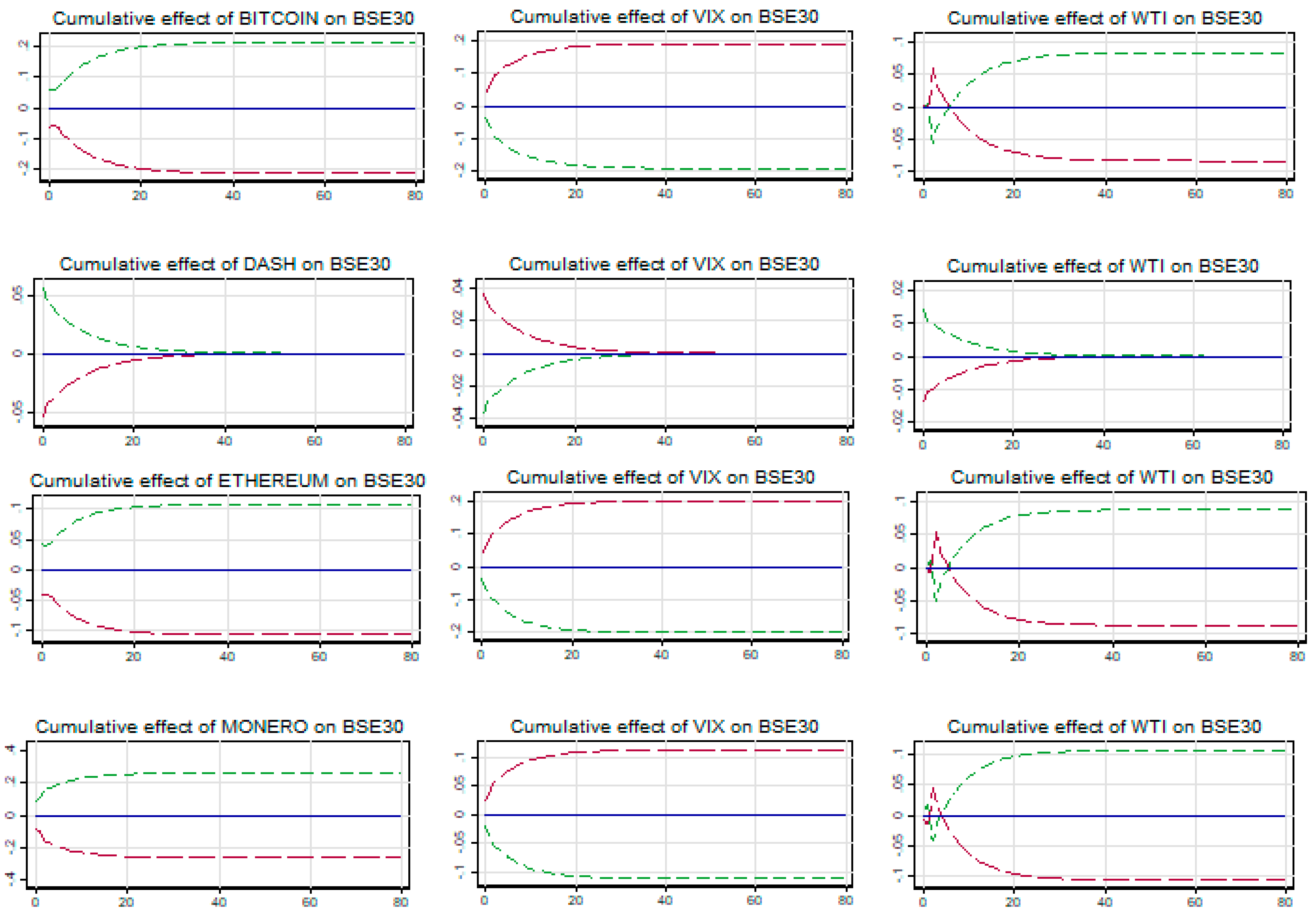
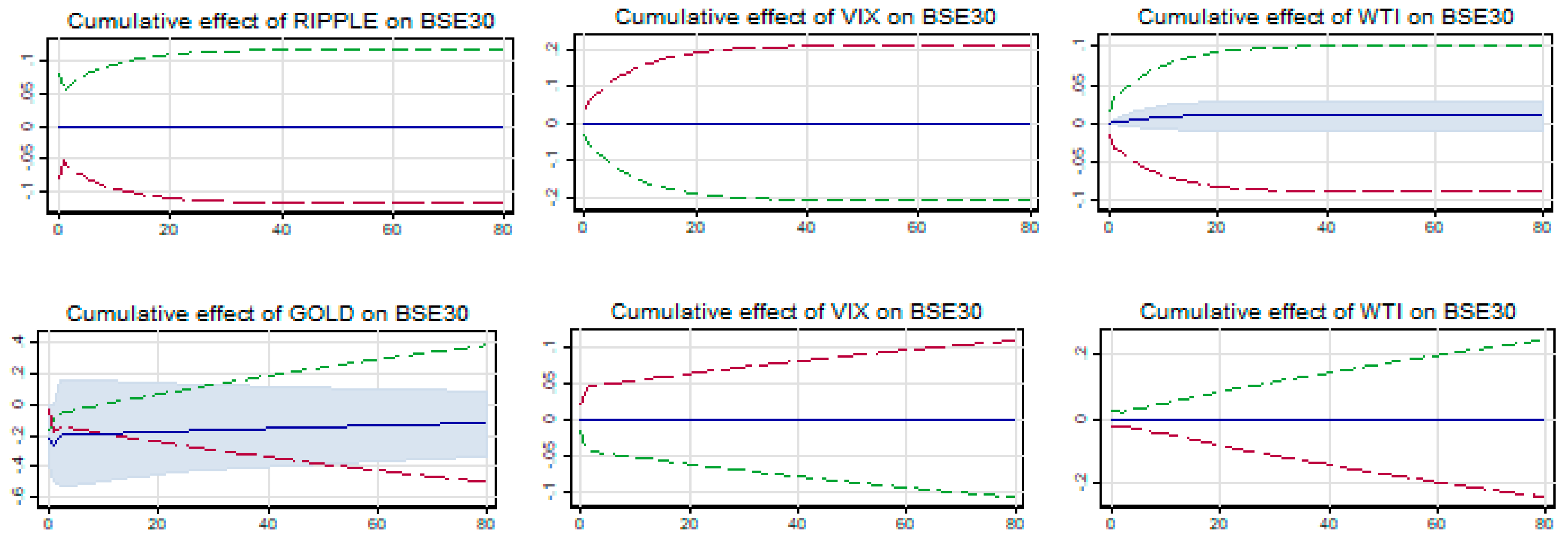
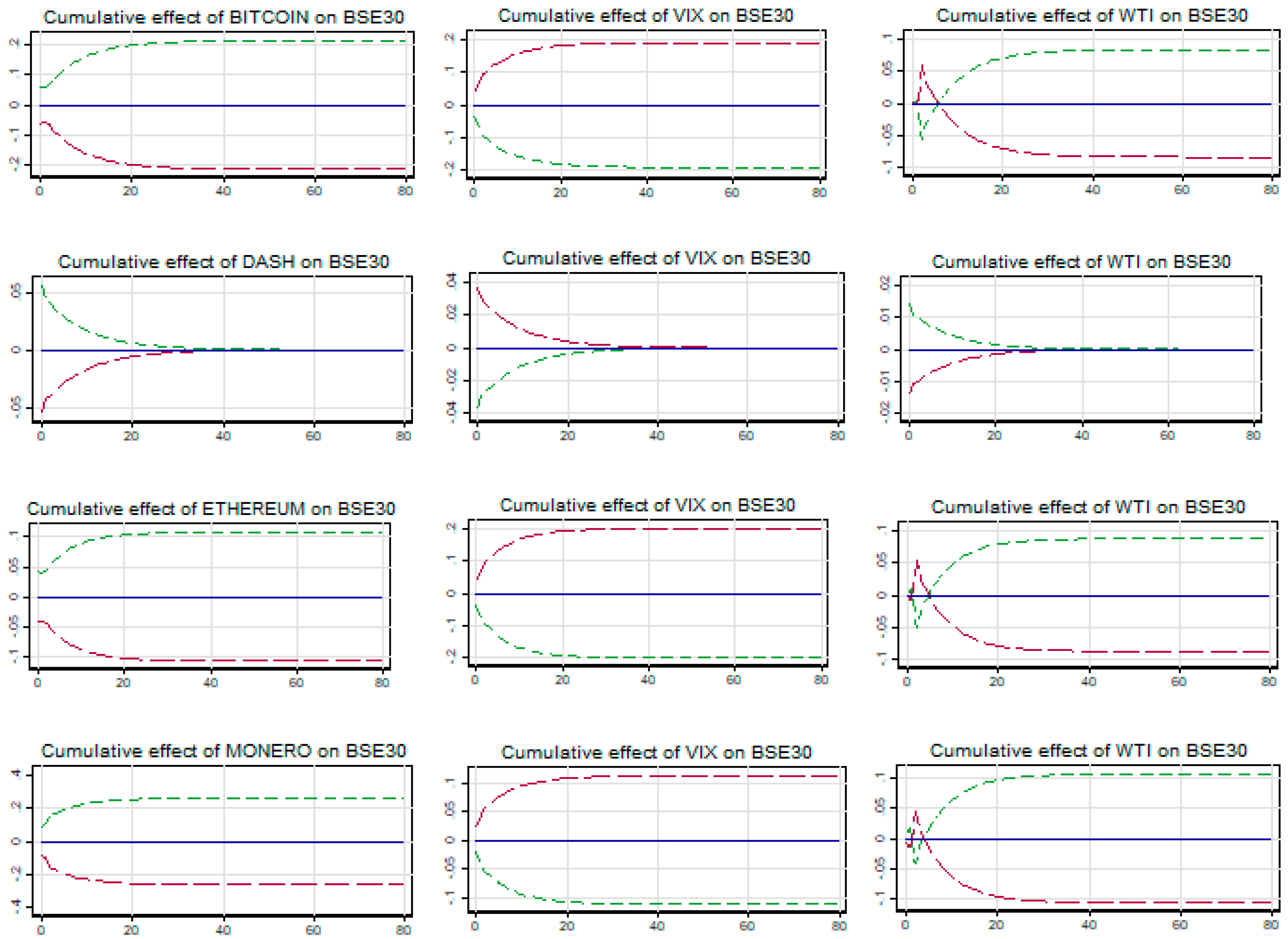
As evidenced from the results presented in Table 5, during the pre-COVID-19 crisis period, long-term symmetric and short-term asymmetric relationships are found between BSE Sensex and gold4. The long-run cointegrating coefficient is significantly positive, thus rejecting any safe haven opportunity of gold for BSE Sensex. It is also confirmed by the cumulative multiplier graph in Figure 1 displaying a highly persistent impact of shock from short-term changes in the gold price on the BSE index, which disturbs the long-run cointegrating equilibrium.

Table 5.
Estimation results for BSE before COVID-19.
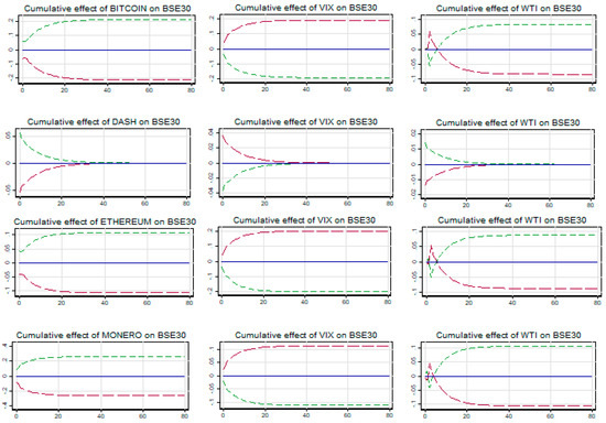
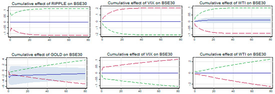
Figure 1.
Cumulative effect of cryptos and gold on BSE30.
4.1.2. BVSP
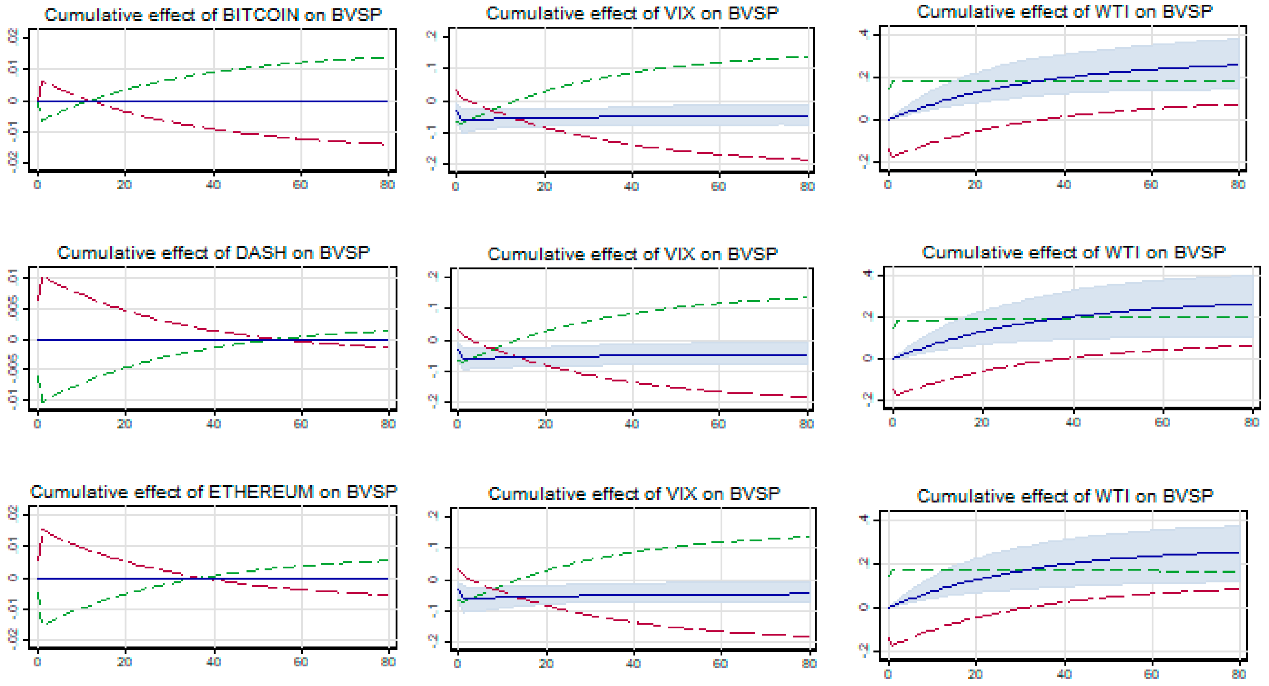
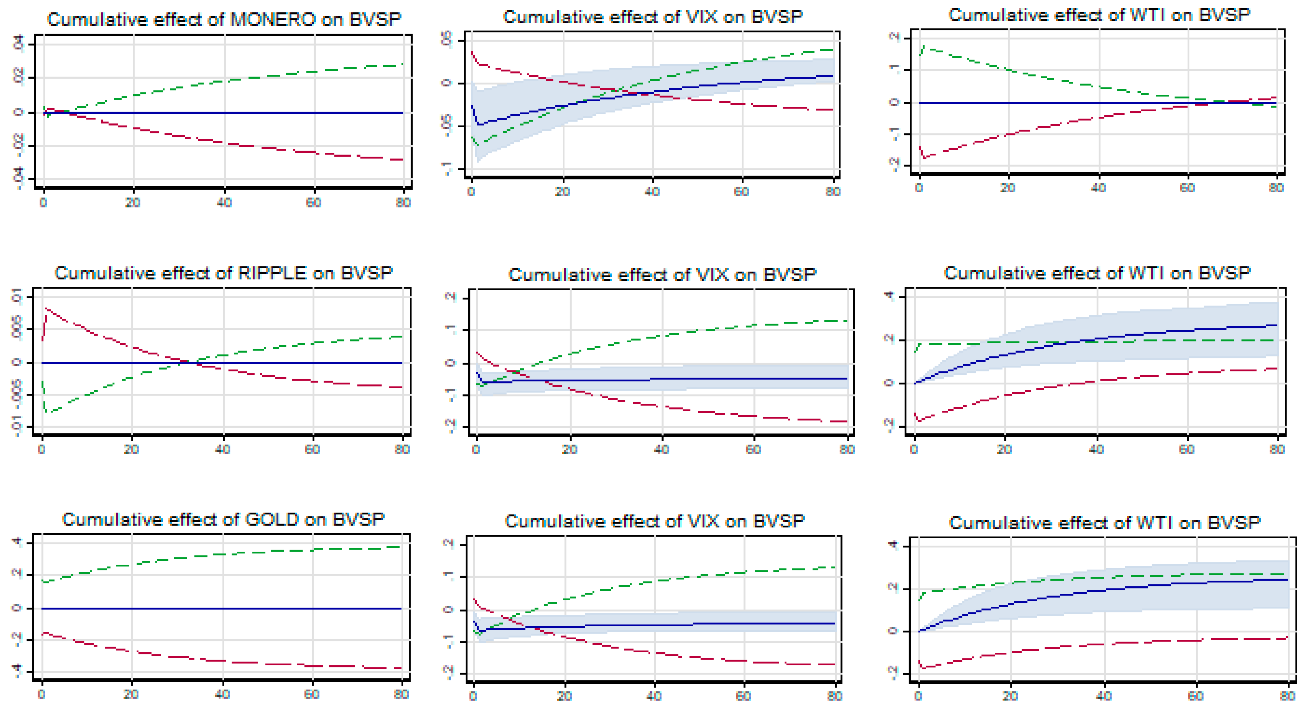
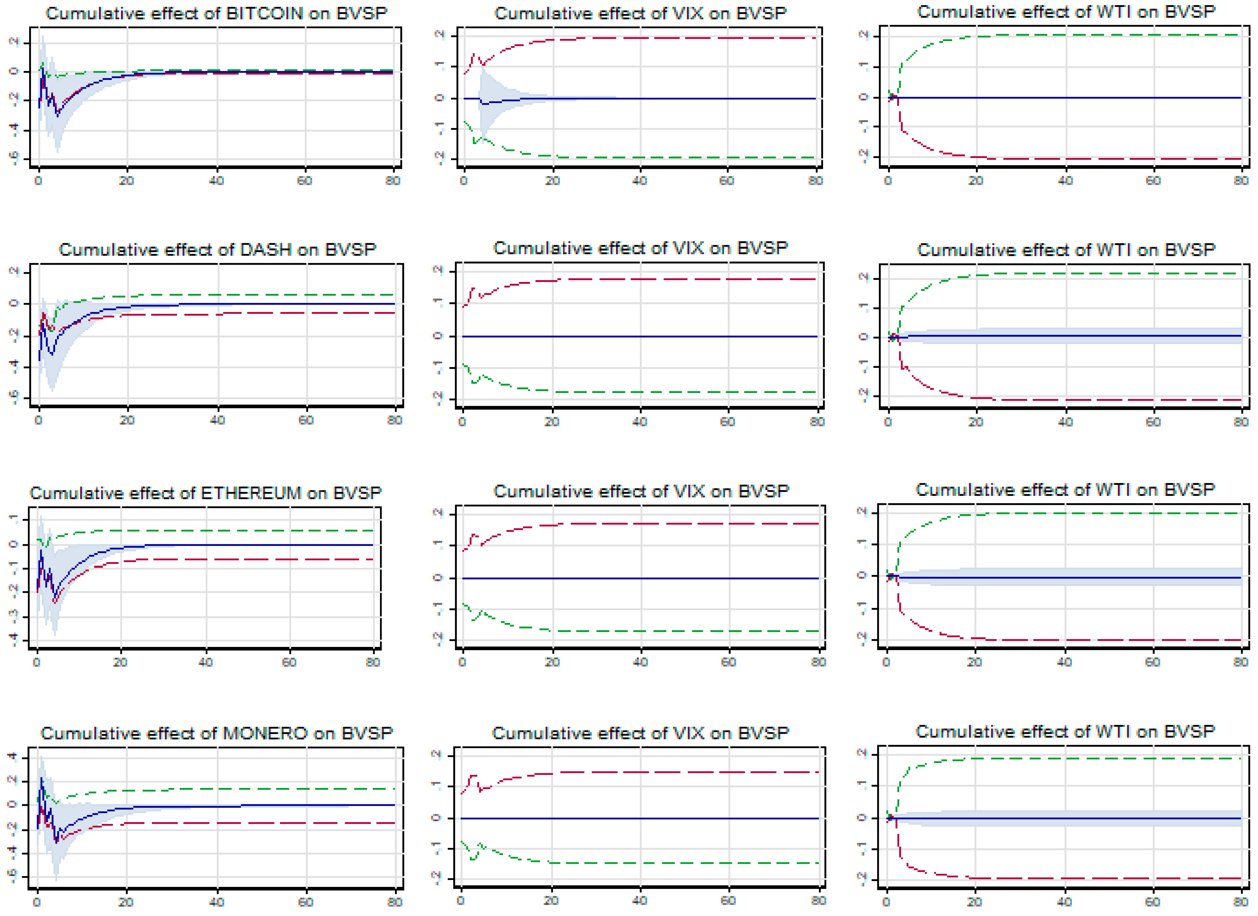
The pre-COVID-19 crisis relationship between BVSP and all five cryptocurrencies together with gold is symmetric both in the long and short run as evidenced from Table 6. The insignificant long-term cointegrating coefficient (LX) with Bitcoin, Dash, Ethereum, and Ripple reveals a weak safe haven opportunity. However, the multiplier graph in Figure 2 shows that the safe haven relationship is affected by short-term changes in cryptocurrency prices. However, gold and Monero are found to be unsuitable for being a safe haven for BVSP.

Table 6.
Estimation results for BSVP before COVID-19.


Figure 2.
Cumulative effects of cryptos and gold on BVSP.
4.1.3. JSE 40
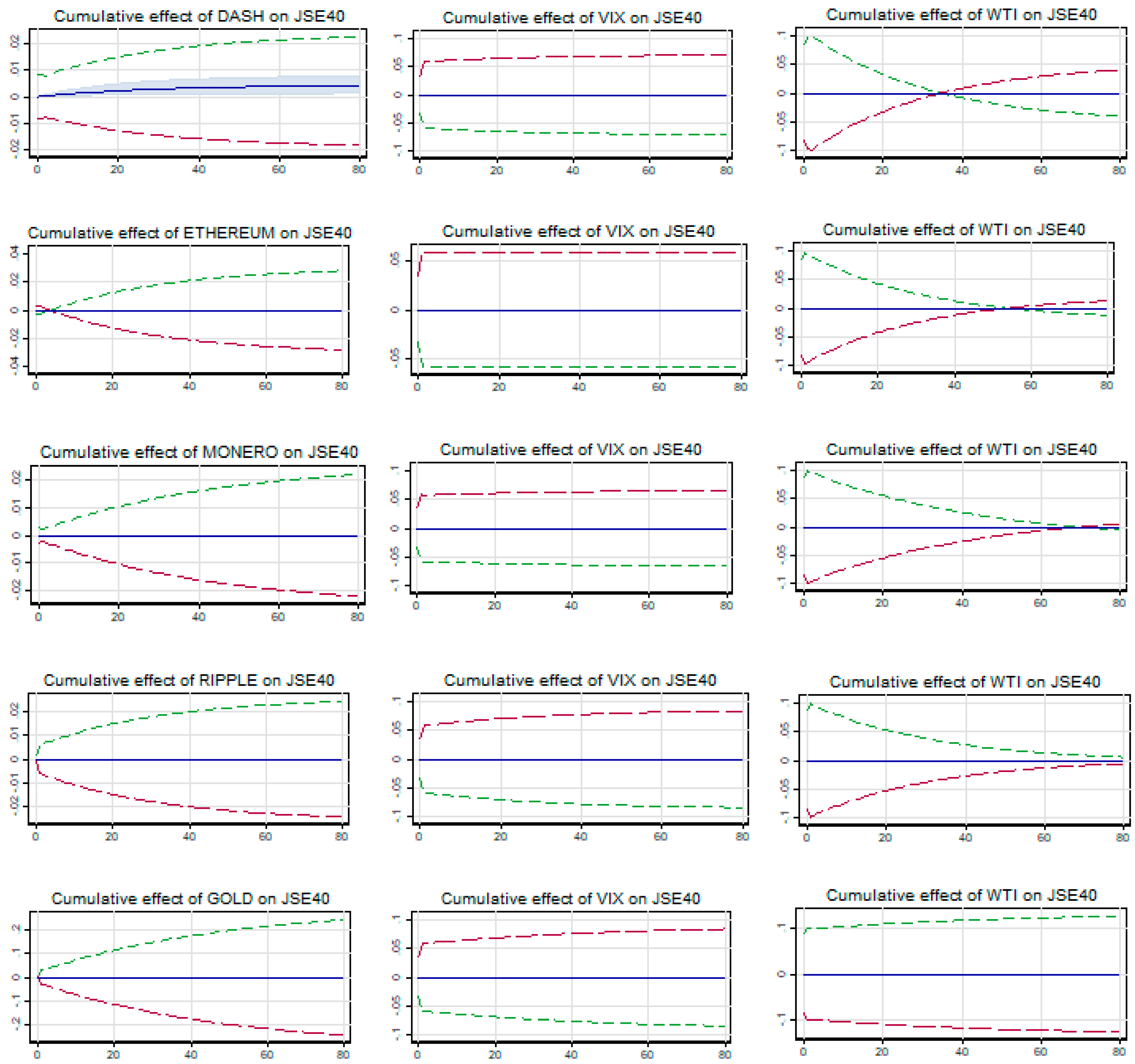
The pre-crisis relationship is symmetric between JSE 40 and three cryptocurrencies, namely, Ethereum, Monero, and Ripple, and gold both in the long and short run as seen from the results in Table 7. However, for Bitcoin and Dash it is symmetric (asymmetric) in the short (long) run. The long-term cointegrating coefficient (LX) is positive and significant across all five cryptocurrencies, thus declining any safe haven opportunity. However, gold is found to be a weak safe haven as the long-term cointegrating coefficient (LX) is negative but not significant. As far as sustainability of the long-term cointegrating relationship is concerned, it is unsustainable as evidenced from the cumulative graph in Figure 3 for all five cryptocurrencies including gold.

Table 7.
Estimation results for JSE 40 before COVID-19.


Figure 3.
Cumulative effects of cryptos and gold on JSE40.
4.1.4. SSE
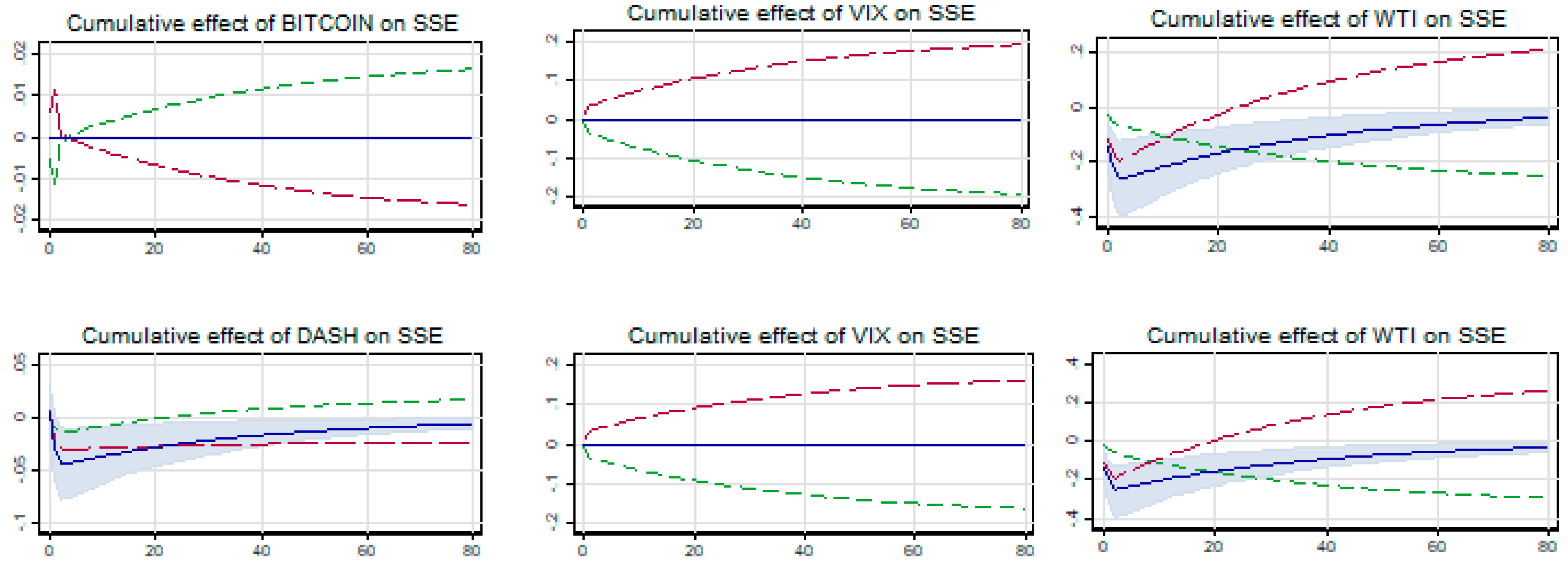
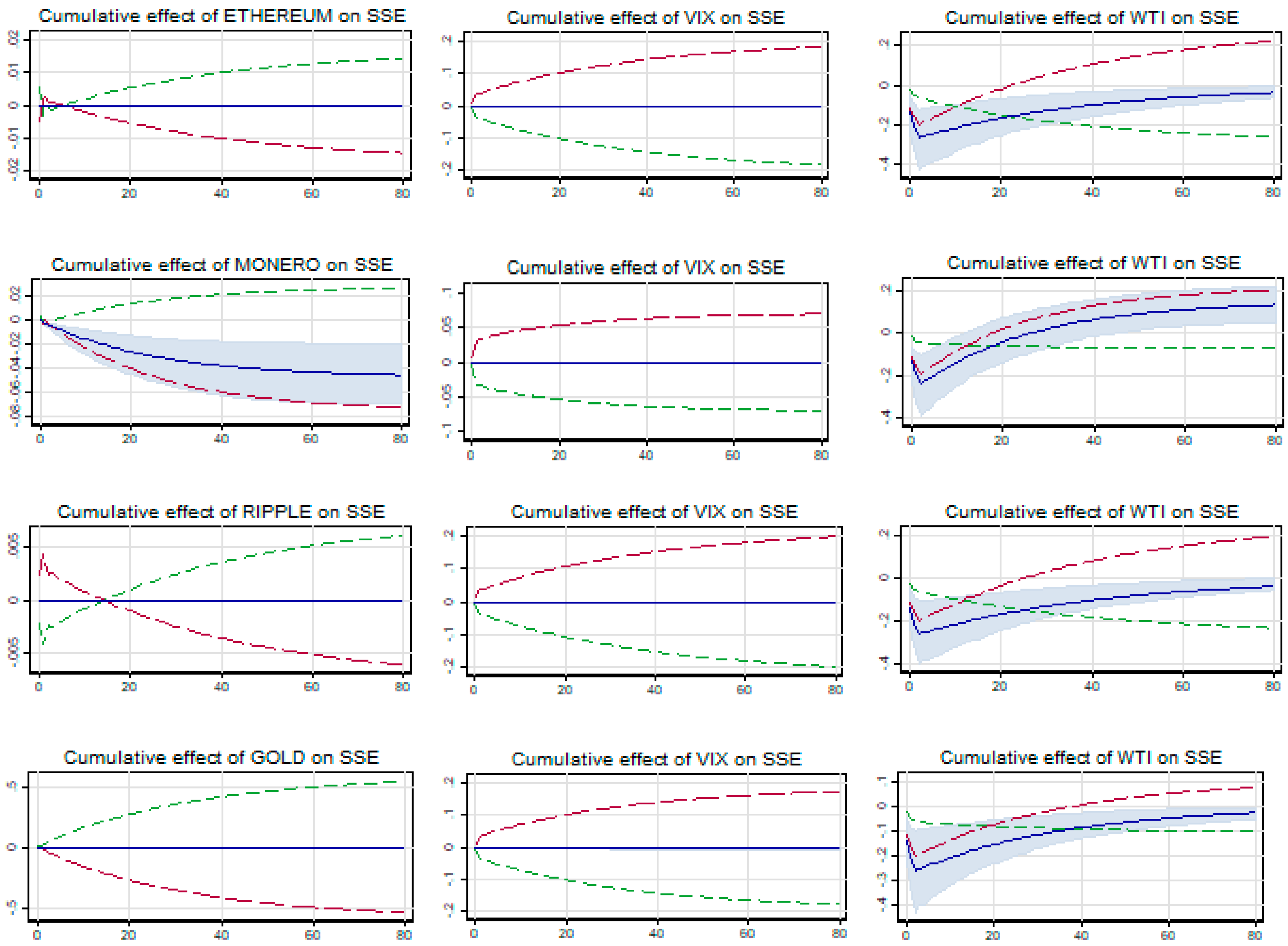
Excepting Dash and Monero, other three cryptocurrencies including gold share a symmetric relationship with SSE both in the long and short run. Dash (Monero) is symmetrically (asymmetrically) related to SSE in the long term and asymmetrically (symmetrically) in the short term during the pre-crisis period as shown by the results in Table 8. Looking at the long-term cointegrating coefficient, it is positive and significant for Dash and gold, thus denouncing any safe haven relationship with SSE. No significant cointegrating (LX) relationship between SSE and Bitcoin, Ethereum, and Ripple signifies a weak safe haven opportunity. Monero is the only cryptocurrency in the pre-crisis period which is a strong safe haven for SSE as the cumulative cointegrating coefficient (LX) is significantly negative. However, as far as sustainability of the safe haven is concerned, as evidenced from Figure 4, except in case of Dash, it is unsustainable as the long-term cointegrating relationship is impacted by short-term shocks from cryptocurrencies and the impact is highly persistent.

Table 8.
Estimation results for SSE before COVID-19.


Figure 4.
Cumulative effects of cryptos and gold on SSE.
4.1.5. RTSI
As evidenced from Table 9, RTSI is found to be symmetrically related to Ethereum, Monero, and gold in the short run, but in the long run it is asymmetrically (symmetrically) related to Monero (Ethereum and gold)5. The insignificant long-term cointegrating relationship (i.e., Lx) in the case of Ethereum and gold does establish a weak safe haven opportunity with RTSI. The cumulative net cointegrating coefficient is significantly negative for Monero, thus signifying a strong safe haven opportunity. However, as evidenced from the cumulative multiplier graph presented in Figure 5, the cointegrating relationship is getting affected by the short-term shocks from unit changes in cryptocurrency during the pre-COVID-19 crisis period and the impact is highly persistent. Thus, it questions the sustainability of the safe haven property of both Ethereum and Monero.

Table 9.
Estimation results for RTSI before COVID-19.
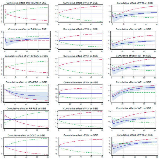
Figure 5.
Cumulative effects of cryptos and gold on RTSI.
4.2. Empirical Analysis of Safe Haven Properties of Cryptocurrencies during the COVID-19 Crisis Period
4.2.1. BSE
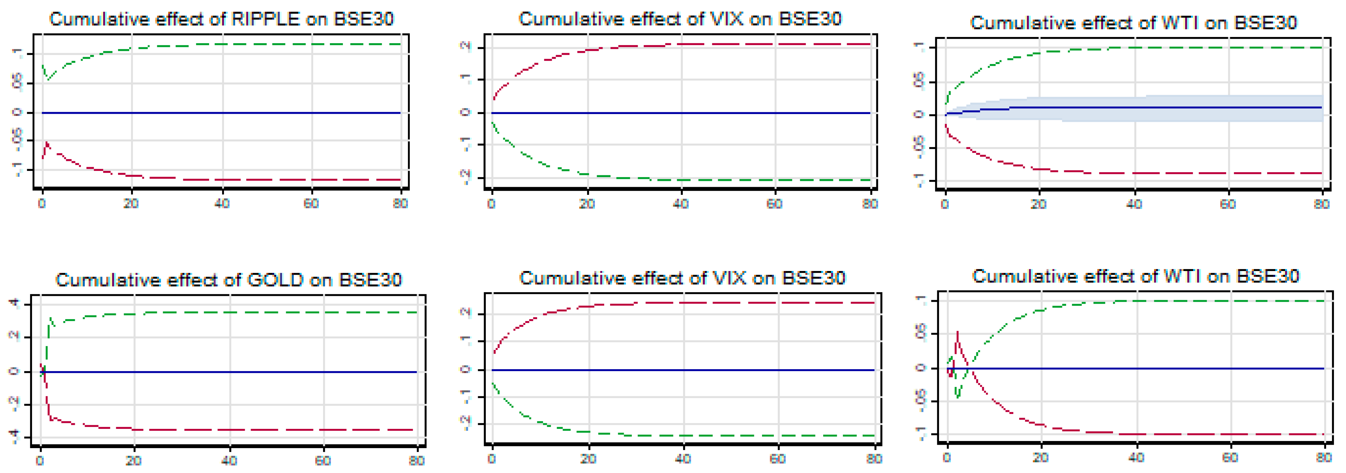
No asymmetric relationship was found between the BSE Sensex and all five cryptocurrencies along with gold, both in the long and short run as evidenced from the results in Table 10. The positive and significant long-term cointegrating coefficient LX rejects the safe haven opportunity of Bitcoin, Ethereum, and Monero, and also gold for BSE Sensex. However, no significant cointegrating relationship with Dash and Ripple implies a weak safe haven opportunity for BSE Sensex. Although both Dash and Ripple are shown to be the safe haven for BSE Sensex during the COVID-19 financial crisis, its effectiveness however depends on the sustainability of this relationship to any short-term shocks from both cryptocurrencies. The cumulative multiplier graph (see Figure 6) shows the moderate impact on BSE Sensex of changes if Dash gets corrected and restored back to the cointegrating relationship within 28–30 days of the impact. However, in the case of Ripple, the impact is persistent, and thus any short-term impact on cointegrating relationships due to shocks from Ripple are not restored. Therefore, it can be concluded that during financial crisis, Dash acts as a weak safe haven for investors in BSE Sensex.

Table 10.
Estimation results for BSE during COVID-19.
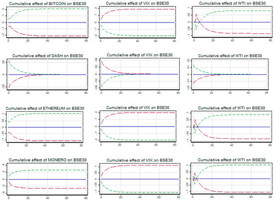
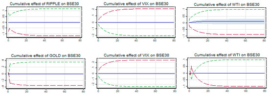
Figure 6.
Cumulative effects of cryptos and gold on BSE30.
4.2.2. BVSP
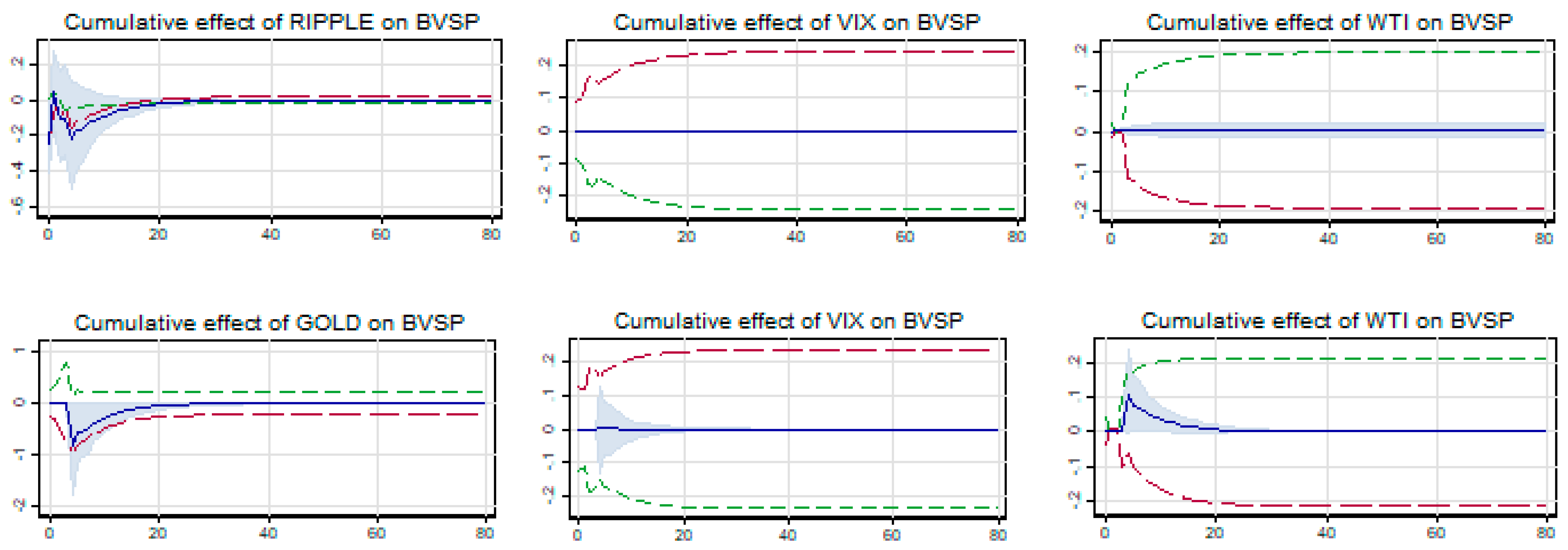
The results in Table 11 show that all five cryptocurrencies share asymmetric (symmetric) relationships in the short (long) run with BVSP. However, gold shares a symmetric relationship both in the short and long run. Since no long-term cointegrating coefficients are significant, including even gold, it establishes a weak safe haven property with BVSP during the COVID-19 financial crisis. However, it needs to be checked how sustainable this safe haven relationship is to short-term shocks from changes in prices in safe haven assets. The cumulative multiplier graphs presented in Figure 7 show that the impact of short-term shocks from safe haven assets, including gold, on BVSP is negative. Further, the impact does not persist long, as it is evident that it takes around 4–5 days’ time to adjust towards the long-term cointegrating relationship. Thus, all the five cryptocurrencies and gold are sustainable safe havens for BVSP during the financial crisis of COVID-19.

Table 11.
Estimation results for BVSP during COVID-19.

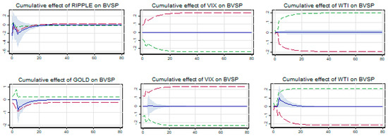
Figure 7.
Cumulative effects of cryptos and gold on BVSP.
4.2.3. JSE 40
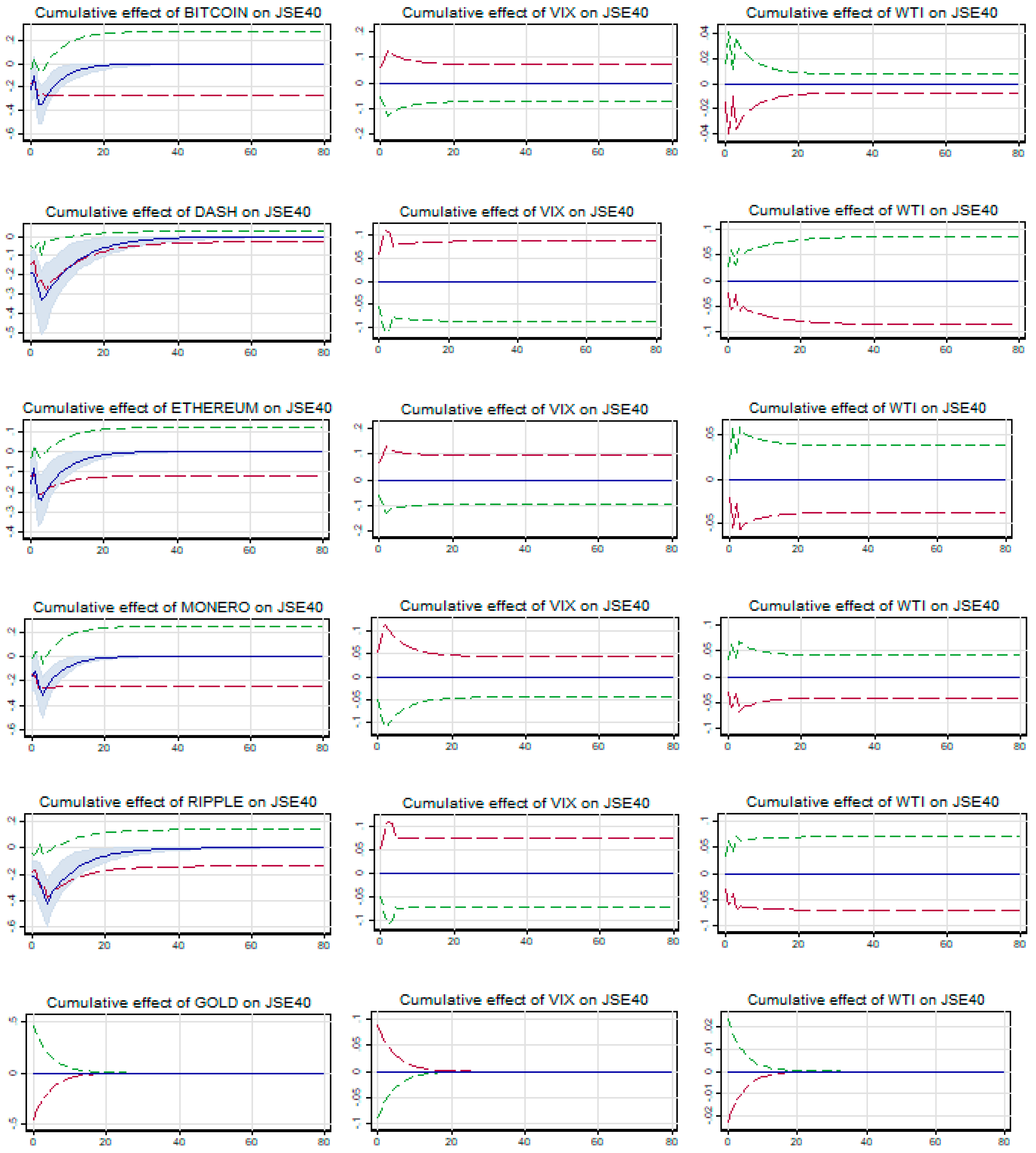
JSE 40 shares a short-term (long-term) asymmetric (symmetric) relationship with all five cryptocurrencies as evidenced from the results presented in Table 12. However, the relationship with gold is symmetric both in the long and short run. Since the long-term cointegrating coefficients (LX) of Bitcoin, Ethereum, Monero, and also gold are significantly positive, it rejects the possibility of any safe haven opportunities. However, a weak safe haven is found with Dash and Ripple. The sustainability of this safe haven opportunity provided by Dash and Ripple can be understood from the cumulative multiplier graph presented in Figure 8. First, the short-term negative impact is observed for unit changes in both Dash and Ripple. However, the status quo gets restored within 20 days (30 days) in the case of Dash (Ripple). Thus, a safe haven for JSE 30 during crisis is more sustainable with Dash than Ripple.

Table 12.
Estimation results for JSE 40 during COVID-19.

Figure 8.
Cumulative effects of cryptos and gold on JSE40.
4.2.4. SSE
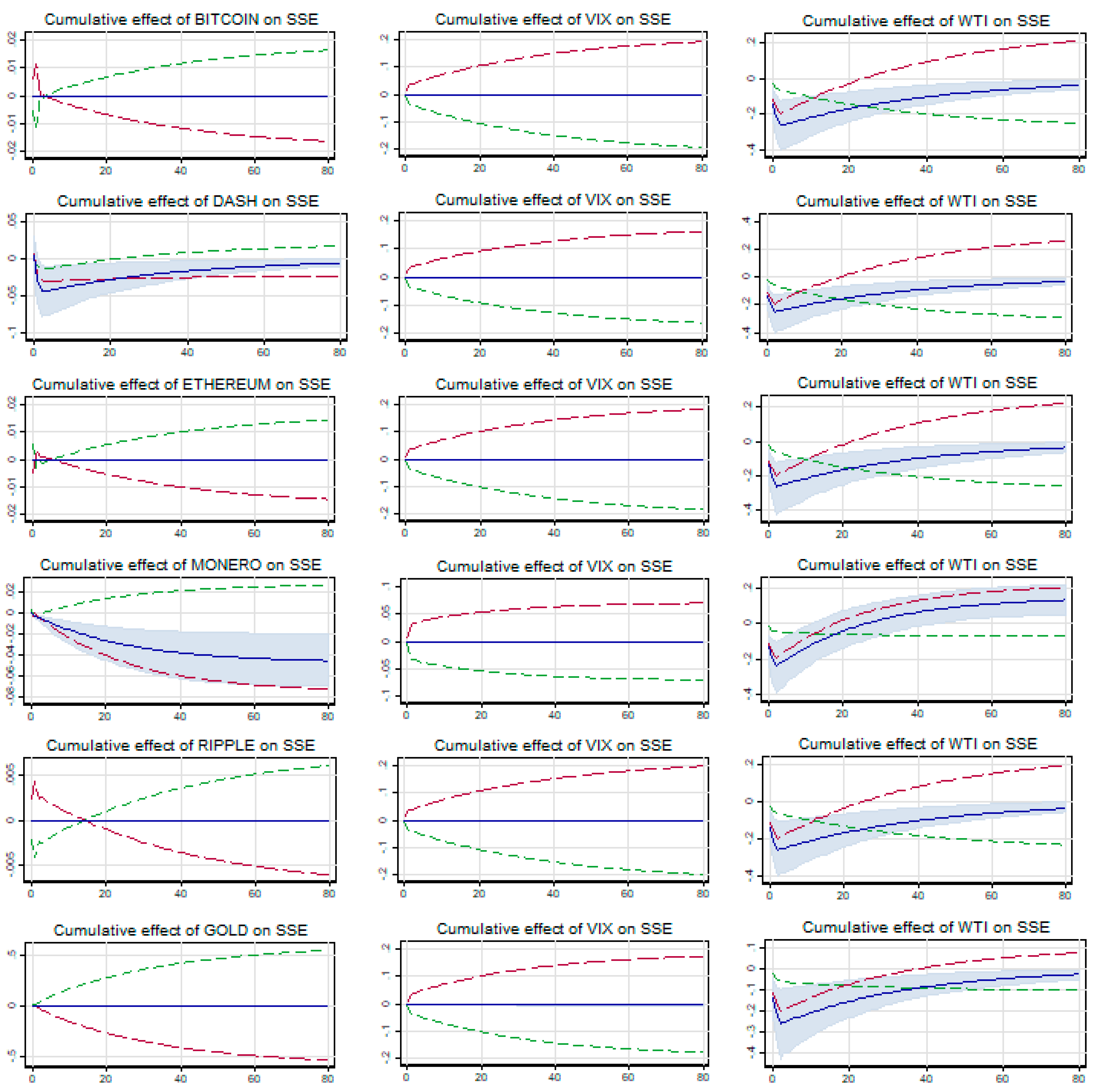
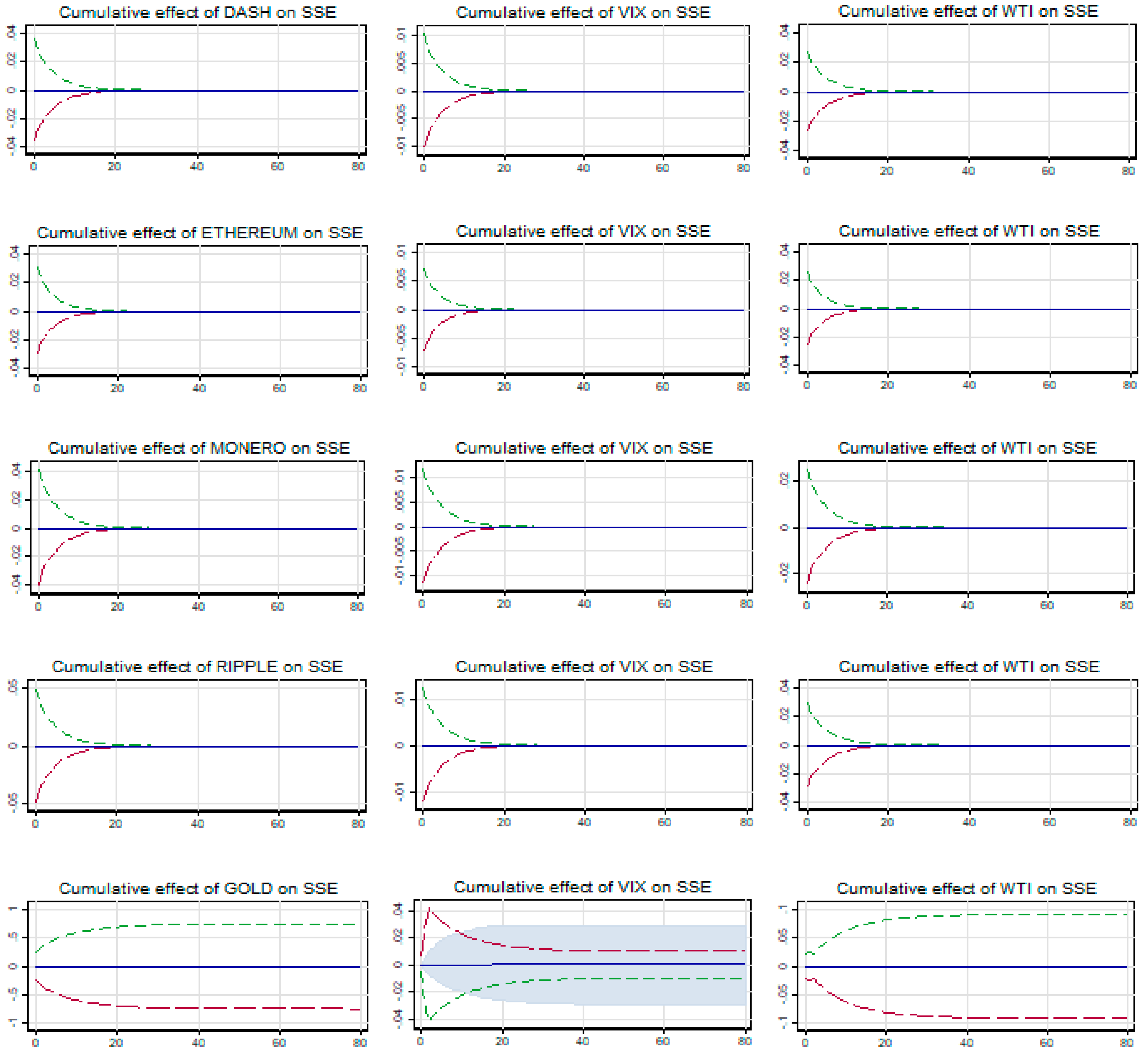
The relationship between SSE and all five cryptocurrencies is asymmetric (symmetric) in long term (short term) as evidenced from the results in Table 13. However, the relationship is reverse in case of gold, i.e., short-term asymmetry and long-term symmetry. The long-term asymmetry could be ascribed only to negative changes in cryptocurrencies as no impact is visible for any positive changes. While the long-term positive cointegrating coefficient is not significant, its negative counterpart is significant for all five cryptocurrencies. Therefore, it establishes a strong safe haven opportunity for SSE in the COVID-19 crisis period. At the same time, as the long-term cointegrating coefficient of gold is significantly positive, it rejects any kind of safe haven opportunity with SSE in this crisis period. Further, as evidenced from the cumulative multiplier graph (Figure 9), it shows the sustainability of this safe haven relationship between SSE and all five cryptocurrencies. Because the impact of the short-term shocks due to unit changes in cryptocurrencies is temporary across all cryptocurrencies, the impacts get adjusted towards the equilibrium in 8–10 days. Thus, all five cryptocurrencies could be a safe haven for investors in SSE.

Table 13.
Estimation results for SSE during COVID-19.

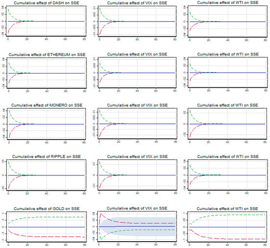
Figure 9.
Cumulative effects of cryptos and gold on SSE.
4.2.5. RTSI
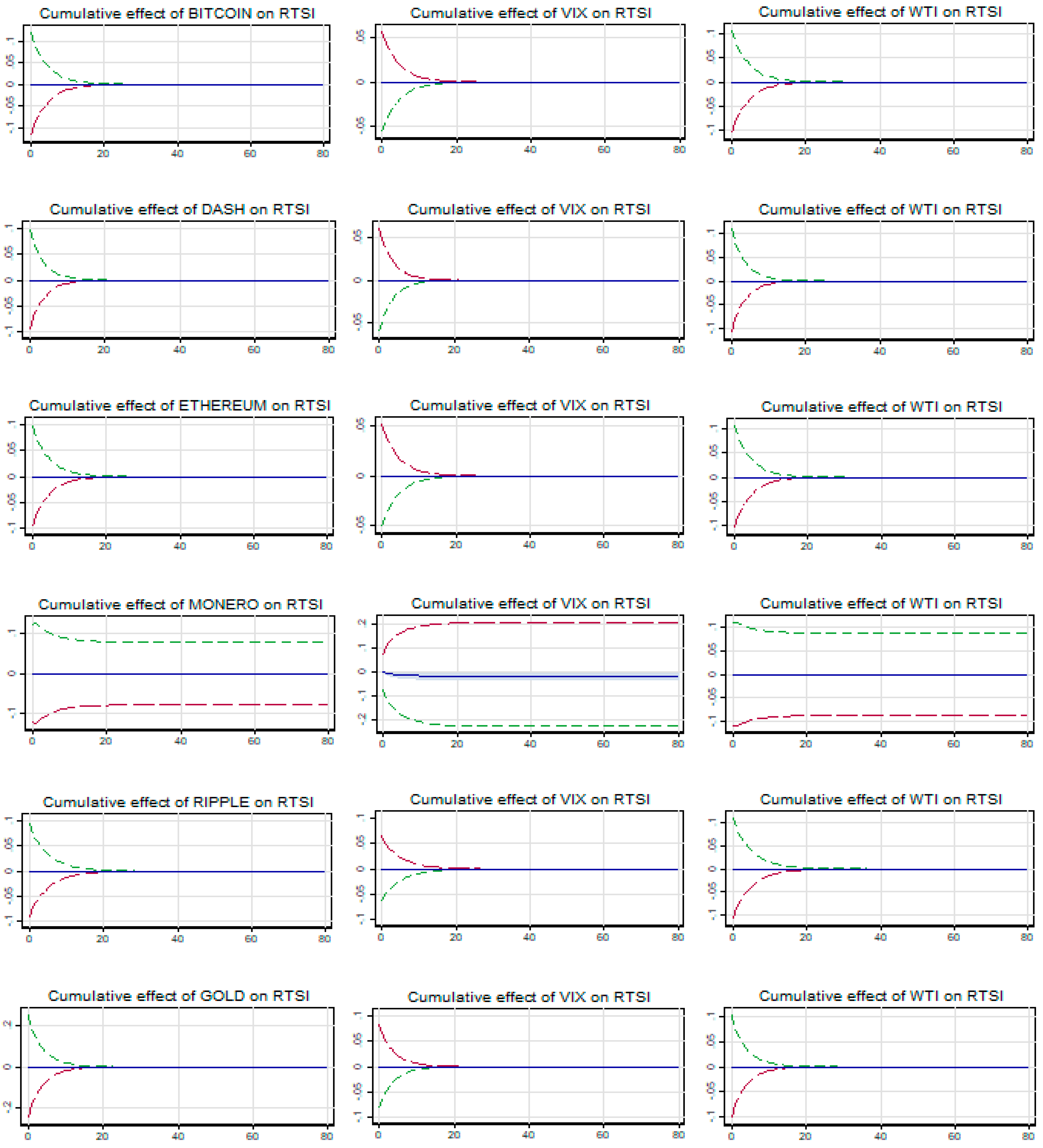
The relationship between RTSI and cryptocurrencies and RTSI and gold are symmetric both in the short and long run as evidenced from the results in Table 14. The long-run cointegrating coefficient is significant and negative with Ethereum, thereby establishing a strong safe haven property. Thus, in the COVID-19 financial market crisis, Ethereum can be part of the RTSI equity portfolio in order to obtain a safe haven benefit. RTSI has a significant and positive relationship with Dash, thus rejecting any kind of safe haven opportunity. However, weak safe haven opportunity is found with Bitcoin, Monero, and Ripple as the long-term cointegrating coefficient is not significant, implying no relationship. Furthermore, gold shows a strong safe haven property with RTSI as the long-term cointegrating coefficient is negative and significant. This safe haven and its stability are further ratified in all cryptocurrencies except Dash and including gold by the cumulative multiplier presented in Figure 10. As evidenced from the graph, any short-term shock on RTSI due to changes in the price of cryptocurrencies does not last long and the status quo is restored in 8–10 days. Thus, except for Dash, the other four cryptocurrencies are safe havens for RTSI during the crisis period.

Table 14.
Estimation results for RTSI during COVID-19.

Figure 10.
Cumulative effects of cryptos and gold on RTSI.
4.3. Comparative Analysis of Pre- and during the COVID-19 Financial Crisis Period
The following Table 15 presents the summary of the pre- and during COVID-19 analysis of the safe haven opportunity of five cryptocurrencies and gold for five BRICS markets.

Table 15.
Summary of the safe haven analysis.
A few important findings are evidenced from Table 15. First, the relationship dynamics both in the short and long run are changing during the crisis period. That justifies our study using a nonlinear and asymmetric model before and during the COVID-19 pandemic crisis. Second, Dash and Ripple were found to be suitable safe havens for all five markets during the COVID-19 crisis period. Third, for BVSP, SSE, and RTSI, almost all cryptocurrencies are safe havens during the financial crisis. Fourth, gold was found to be a suitable safe haven only for BVSP and RTSI during the crisis period. Our results are in contrast to the findings of Wang et al. (2019b), wherein cryptocurrencies were not found to be a safe haven for developing markets, including BRICS countries. However, our findings are relatively in line with Corbet et al. (2018) who found diversification opportunity in Bitcoin, Ripple, and Litecoin because of low linkages with traditional asset classes. As far as gold as a safe haven asset is concerned, it is relatively in line with Aftab et al. (2019).
The implications of our results are manifold for portfolio managers and traders as well. The index fund managers of BVSP, SSE, and RTSI (all five BRICS markets) could use all these five cryptocurrencies (Dash and Ripple) as safe haven assets in the COVID-19 crisis period to protect the value of the portfolio. Further, based on cointegrating relationship dynamics between cryptocurrencies and BRICS indices, traders can design and implement spread strategies. As far as market regulators and policy makers are concerned, in the case of positive long- and short-term relationships, policy measures could be initiated to check spillover of volatility from the cryptocurrencies market. The study is limited to five cryptocurrencies and five developing markets, namely, BRICS markets. In a future study, the NARDL model could be applied in the developed and frontier markets, considering more cryptocurrencies.
5. Conclusions and Policy Recommendations
The current crisis in stock markets around the world brought about by the COVID-19 pandemic made investors search for a sustainable hiding space for their investments. The crisis was not only confined to the stock market but was spread across the commodities market also. Over a period of time following certain developments, cryptocurrencies have attracted the attention of portfolio investors. In this study, we have investigated the safe haven properties of the top five cryptocurrencies together with gold for BRICS markets in a nonlinear and asymmetric framework using NARDL methodology before and during the COVID-19 financial crisis. Our results show that, in a nonlinear and asymmetric framework, the relationship dynamics between stock market returns and crypto returns both in the short and long run are changing during the COVID-19 crisis period. Dash and Ripple are found to be a sustainable safe haven for all five markets. However, all five cryptocurrencies are found to be a sustainable safe haven for three emerging markets, namely, BVSP, SSE, and RTSI, during the financial crisis. In a comparative framework, gold is found to be a suitable safe haven only for BVSP and RTSI. Thus, portfolio managers, such as for index funds, may consider the few eligible cryptocurrencies for their inclusion into the portfolio. The speculators present in both stock and crypto markets may aim for a spread strategy to improve their portfolio return.
Author Contributions
Data curation, A.J.; Formal analysis, A.L.; Software, A.L.; Writing—original draft, S.K.J.; Writing—review & editing, A.J. and A.L. All authors have read and agreed to the published version of the manuscript.
Funding
This research received no external funding.
Informed Consent Statement
Informed consent was obtained from all subjects involved in the study.
Data Availability Statement
Data are available upon request from authors.
Conflicts of Interest
The authors declare no conflict of interest.
Note
| 1 | The volatility index across the stock markets of developing and developed countries made new historic highs. |
| 2 | We have followed Phillip et al. (2018) and selected the top five cryptocurrencies based on market capitalisation as at July 2017. |
| 3 | On 30 January 2020, the World Health Organisation (WHO) declared COVID-19 as a “Public Health Emergency of International Concern”. |
| 4 | The NARDL model is found to be unsuitable for the study of safe havens between BSE Sensex and all five cryptocurrencies during the pre-COVID-19 crisis period as the estimated speed of the adjustment parameter is not significantly negative. |
| 5 | For Bitcoin, Dash, and Ethereum, NARDL is found unsuitable for the estimation. |
References
- Aftab, Muhammad, Syed Zulfiqar Ali Shah, and Izlin Ismail. 2019. Does Gold Act as a Hedge or a Safe Haven against Equity and Currency in Asia? Global Business Review 20: 105–18. [Google Scholar] [CrossRef]
- Baur, Dirk G., and Brian M. Lucey. 2010. Is gold a hedge or a safe haven? An analysis of stocks, bonds and gold. Financial Review 45: 217–29. [Google Scholar] [CrossRef]
- Baur, Dirk G., and Thomas K. McDermott. 2010. Is gold a safe haven? International evidence. Journal of Banking & Finance 34: 1886–98. [Google Scholar]
- Bouri, Elie, Peter Molnár, Georges Azzi, David Roubaud, and Lars Ivar Hagfors. 2017. On the hedge and safe haven properties of Bitcoin: Is it really more than a diversifier? Finance Research Letters 20: 192–98. [Google Scholar] [CrossRef]
- Bouri, Elie, Rangan Gupta, Amine Lahiani, and Muhammad Shahbaz. 2018. Testing for asymmetric short- and long-run relationships between bitcoin, aggregate commodity and gold prices. Resources Policy 57: 224–35. [Google Scholar] [CrossRef] [Green Version]
- Bouri, Elie, Syed Jawad Hussain Shahzad, David Roubaud, Ladislav Kristoufek, and Brian Lucey. 2020. Bitcoin, gold, and commodities as safe havens for stocks: New insight through wavelet analysis. The Quarterly Review of Economics and Finance 77: 156–64. [Google Scholar] [CrossRef]
- Conlon, Thomas, and Richard McGee. 2020. Safe Haven or Risky Hazard? Bitcoin during the COVID-19 Bear Market. Finance Research Letters 35: 101607. [Google Scholar] [CrossRef]
- Corbet, Shaen, Andrew Meegan, Charles Larkin, Brian Lucey, and Larisa Yarovaya. 2018. Exploring the dynamic relationships between cryptocurrencies and other financial assets. Economics Letters 165: 28–34. [Google Scholar] [CrossRef] [Green Version]
- Corbet, Shaen, Douglas J. Cumming, Brian M. Lucey, Maurice Peat, and Samuel Vigne. 2019. Investigating the dynamics between price volatility, price discovery, and criminality in cryptocurrency markets. Price Discovery, and Criminality in Cryptocurrency Markets. Available online: https://ssrn.com/abstract=3384707 (accessed on 3 May 2019).
- Dyhrberg, Anne Haubo. 2016. Bitcoin, gold and the dollar–A GARCH volatility analysis. Finance Research Letters 16: 85–92. [Google Scholar] [CrossRef] [Green Version]
- Gajardo, Gabriel, Werner D. Kristjanpoller, and Marcel Minutolo. 2018. Does Bitcoin exhibit the same asymmetric multifractal cross-correlations with crude oil, gold and DJIA as the Euro, Great British Pound and Yen? Chaos, Solitons & Fractals 109: 195–205. [Google Scholar]
- Garcia-Jorcano, Laura, and Sonia Benito Muela. 2020. Studying the properties of the Bitcoin as a diversifying and hedging asset through a copula analysis: Constant and time-varying. Research in International Business and Finance 54: 101300. [Google Scholar] [CrossRef]
- Ghorbel, Achraf, and Ahmed Jeribi. 2021. Investigating the relationship between volatilities of cryptocurrencies and other financial assets. Decisions in Economics and Finance, 1–27. [Google Scholar] [CrossRef]
- González, Maria de la O., Francisco Jareño, and Frank S. Skinner. 2021. Asymmetric interdependencies between large capital cryptocurrency and gold returns during the COVID-19 pandemic. International Review of Financial Analysis 76: 101778. [Google Scholar] [CrossRef]
- Jareño, Francisco, María de la O. González, Marta Tolentino, and Karen Sierra. 2020. Bitcoin and gold price returns: A quantile regression and NARDL analysis. Resources Policy 67: 101666. [Google Scholar] [CrossRef]
- Jeribi, Ahmed, and Mohamed Fakhfekh. 2021. Portfolio management and dependence structure between cryptocurrencies and traditional assets: Evidence from FIEGARCH-EVT-Copula. Journal of Asset Management 22: 224–39. [Google Scholar] [CrossRef]
- Johansen, Soren. 1992. Determination of Cointegration Rank in the Presence of a Linear Trend. Oxford Bulletin of Economics and Statistics 54: 383–97. [Google Scholar] [CrossRef]
- Kajtazi, Anton, and Andrea Moro. 2019. The role of bitcoin in well diversified portfolios: A comparative global study. International Review of Financial Analysis 61: 143–57. [Google Scholar] [CrossRef] [Green Version]
- Klein, Tony. 2017. Dynamic correlation of precious metals and flight-to-quality in developed markets. Finance Research Letters 23: 283–90. [Google Scholar] [CrossRef]
- Klein, Tony, Hien Pham Thu, and Thomas Walther. 2018. Bitcoin is not the New Gold–A comparison of volatility, correlation, and portfolio performance. International Review of Financial Analysis 59: 105–16. [Google Scholar] [CrossRef]
- Kliber, Agata, Paweł Marszałek, Ida Musiałkowska, and Katarzyna Świerczyńska. 2019. Bitcoin: Safe haven, hedge or diversifier? Perception of bitcoin in the context of a country’s economic situation: A stochastic volatility approach. Physica A: Statistical Mechanics and its Applications 524: 246–57. [Google Scholar] [CrossRef]
- Kristoufek, Ladislav. 2015. What are the main drivers of the Bitcoin price? Evidence from wavelet coherence analysis. PLoS ONE 10: e0123923. [Google Scholar] [CrossRef]
- Lahiani, Amine, and Nabila Boukef Jlassi. 2021. Nonlinear tail dependence in cryptocurrency-stock market returns: The role of Bitcoin futures. Research in International Business and Finance 56: 101351. [Google Scholar] [CrossRef]
- Luther, William J., and Alexander W. Salter. 2017. Bitcoin and the bailout. The Quarterly Review of Economics and Finance 66: 50–56. [Google Scholar] [CrossRef]
- Maiti, Moinak, Zoran Grubisic, and Darko B. Vukovic. 2020. Dissecting Tether’s Nonlinear Dynamics during Covid-19. Journal of Open Innovation: Technology, Market, and Complexity 6: 161. [Google Scholar] [CrossRef]
- Pal, Debdatta, and Subrata K. Mitra. 2019. Hedging bitcoin with other financial assets. Finance Research Letters 30: 30–36. [Google Scholar] [CrossRef]
- Perron, Pierre. 1989. The Great Crash, the Oil Price Shock, and the Unit Root Hypothesis. Econometrica 57: 1361–401. [Google Scholar] [CrossRef]
- Pesaran, M. Hashem, Yongcheol Shin, and Richard J. Smith. 2001. Bounds testing approaches to the analysis of level relationships. Journal of Applied Econometrics 16: 289–326. [Google Scholar] [CrossRef]
- Phillip, Andrew, Jennifer SK Chan, and Shelton Peiris. 2018. A new look at Cryptocurrencies. Economics Letters 163: 6–9. [Google Scholar] [CrossRef]
- Shahzad, Syed Jawad Hussain, Elie Bouri, David Roubaud, and Ladislav Kristoufek. 2019. Safe haven, hedge and diversification for G7 stock markets: Gold versus bitcoin. Economic Modelling 87: 212–24. [Google Scholar] [CrossRef]
- Shin, Yongcheol, Byungchul Yu, and Matthew Greenwood-nimmo. 2014. Modelling asymmetric cointegration and dynamic multipliers in a nonlinear ARDL framework. In Festschrift in Honor of Peter Schmidt Econometric Methods and Applications. Edited by R.C. Sickles and W.C. Horrace. New York: Springer, pp. 281–314. [Google Scholar]
- Smales, Lee A. 2018. Bitcoin as a safe haven: Is it even worth considering? Finance Research Letters 30: 385–93. [Google Scholar] [CrossRef]
- Urquhart, Andrew, and Hanxiong Zhang. 2019. Is Bitcoin a hedge or safe haven for currencies? An intraday analysis. International Review of Financial Analysis 63: 49–57. [Google Scholar] [CrossRef]
- Wang, Gangjin, Yanping Tang, Chi Xie, and Shou Chen. 2019a. Is bitcoin a safe haven or a hedging asset? Evidence from China. Journal of Management Science and Engineering 4: 173–88. [Google Scholar] [CrossRef]
- Wang, Pengfei, Wei Zhang, Xiao Li, and Dehua Shen. 2019b. Is cryptocurrency a hedge or a safe haven for international indices? A comprehensive and dynamic perspective. Finance Research Letters 31: 1–18. [Google Scholar] [CrossRef]
- Wei, Wang Chun. 2018. Liquidity and market efficiency in cryptocurrencies. Economics Letters 168: 21–24. [Google Scholar] [CrossRef]
Publisher’s Note: MDPI stays neutral with regard to jurisdictional claims in published maps and institutional affiliations. |
© 2021 by the authors. Licensee MDPI, Basel, Switzerland. This article is an open access article distributed under the terms and conditions of the Creative Commons Attribution (CC BY) license (https://creativecommons.org/licenses/by/4.0/).

