The Determinants of the U.S. Consumer Sentiment: Linear and Nonlinear Models


Abstract
1. Introduction
2. Literature Review
3. Data
- University of Michigan Consumer Sentiment Index is a monthly survey of U.S. consumer confidence levels conducted by the University of Michigan. It is based on telephone surveys that gather information on consumer expectations regarding the overall economy.
- Bloomberg Barometer Startups Global Index measures both the occurrence and level of historical and recent venture activity for U.S.-based startups excluding biotechnology. The index is a gauge of startup activity that equally considers capital raised, deal count, first financings, and exit count.
- Business Confidence Index provides information on future developments, based upon opinion surveys on developments in production, orders, and stocks of finished goods in the industry sector.
- Dow Jones Sustainability United States 40 Index is composed of U.S. sustainability leaders as identified by Sustainable Asset Management (SAM) through a corporate sustainability assessment. The index represents the top 20% of the largest 600 U.S. companies in the Dow Jones Sustainability U.S. Index based on long-term economic, environmental, and social criteria.
- Morgan Stanley Capital International (MSCI) Global Energy Efficiency Index includes developed and emerging market large-, mid-, and smallcap companies that derive 50% or more of their revenues from products and services in energy efficiency.
- MSCI USA ESG leaders index is a capitalization weighted index that provides exposure to companies with high Environmental, Social, and Governance (ESG) performance relative to their sector peers.
- Personal Income in Billions is the income that persons receive in return for their provision of labor, land, and capital used in current production and the net current transfer payments that they receive from business and from government.
- S&P Carbon Efficiency Index is designed to measure the performance of companies in the S&P 500, while overweighting or underweighting those companies that have lower or higher levels of carbon emissions per unit of revenue.
- S&P Consumer Finance Index provides liquid exposure to mortgage real estate investment trusts (REITs), thrifts and mortgage finance companies, diversified and regional banks, consumer finance or data processing services companies trading on U.S. stock exchanges.
- S&P Municipal Bond Education Index consists of bonds in the S&P Municipal Bond Index from the Higher Education and Student Loan Sectors.
- U.S. unemployment rate is defined as the percentage of unemployed people who are currently in the labor force. In order to be in the labor force, a person either must have a job or have looked for work in the last four weeks.
4. Empirical Models and Results
4.1. Multicollinearity Analysis
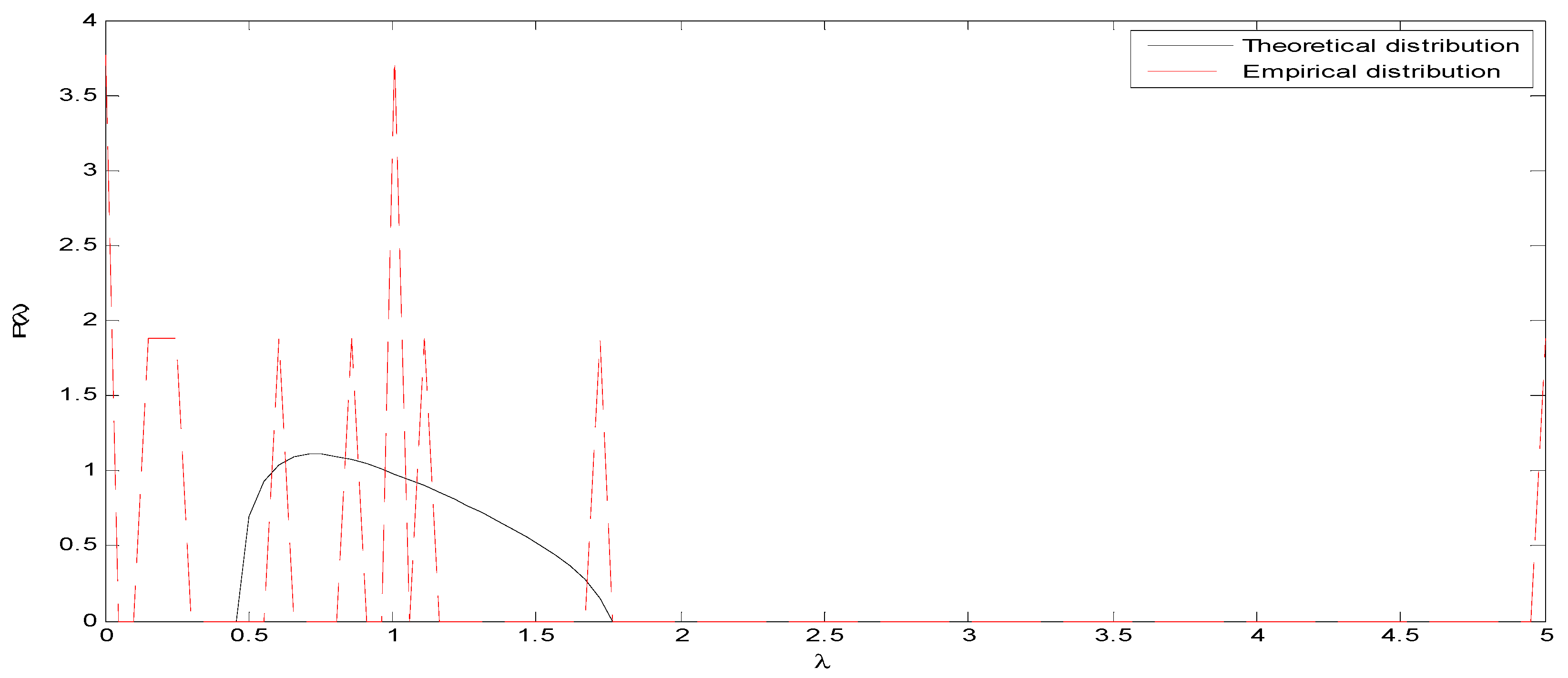
4.2. Random Matrix Theory Analysis
4.3. Regression Analysis
4.4. Regime Switching Model
4.5. Gradient Descent Algorithm
5. Conclusions
Author Contributions
Funding
Acknowledgments
Conflicts of Interest
References
- Akhtar, Shumi, Robert Faff, Barry Oliver, and Avanidhar Subrahmanyam. 2011. The power of bad: The negativity bias in Australian consumer sentiment announcements on stock returns. Journal of Banking & Finance 35: 1239–49. [Google Scholar]
- Baghestani, Hamid, and Polly Palmer. 2017. On the dynamics of US consumer sentiment and economic policy assessment. Applied Economics 49: 227–37. [Google Scholar] [CrossRef]
- Balcilar, Mehmet, Rangan Gupta, and Clement Kyei. 2018. Predicting Stock Returns and Volatility with Investor Sentiment Indices: A Reconsideration Using a Nonparametric Causality-In-Quantiles Test. Bulletin of Economic Research 70: 74–87. [Google Scholar] [CrossRef]
- Baker, Malcolm, and Jeffrey Wurgler. 2006. Investor Sentiment and the Cross-Section of Stock Returns. The Journal of Finance 61: 1645–80. [Google Scholar] [CrossRef]
- Baker, Malcolm, and Jeffrey Wurgler. 2007. Investor Sentiment in the Stock Market. Journal of Economic Perspectives 21: 129–51. [Google Scholar] [CrossRef]
- Bouchaud, Jean-Philippe, and Marc Potters. 2003. Theory of Financial Risk and Derivative Pricing: From Statistical Physics to Risk Management. Cambridge: Cambridge University Press. [Google Scholar]
- Bouteska, Ahmed. 2019. The effect of investor sentiment on market reactions to financial earnings restatements: Lessons from the United States. Journal of Behavioral and Experimental Finance 24: 1–11. [Google Scholar] [CrossRef]
- Cauchy, Augustin. 1847. Méthode générale pour la résolution des systèmes d’équations simultanées. Comptes rendus de l’Académie des Sciences 25: 536–38. [Google Scholar]
- Chung, San-Lin, Chi-Hsiou Hung, and Chung-Ying Yeh. 2012. When does investor sentiment predict stock returns? Journal of Empirical Finance 19: 217–40. [Google Scholar] [CrossRef]
- Cofnas, Abe, ed. 2015. How Business Confidence and Consumer Sentiment Affect the Market. In The Forex Trading Course: A Self-Study Guide to Becoming a Successful Currency Trader. Hoboken: John Wiley & Sons Inc., pp. 51–52. [Google Scholar]
- Dyson, Freeman J. 1971. Distribution of eigenvalues for a class of real symmetric matrices. Revista Mexicana de Fisica 20: 231–37. [Google Scholar]
- Fisher, Kenneth L., and Meir Statman. 2000. Investor Sentiment and Stock Returns. Financial Analyst Journal 56: 16–23. [Google Scholar] [CrossRef]
- Fisher, Lance A., and Hyeon-seung Huh. 2016. On the econometric modelling of consumer sentiment shocks in SVARs. Empirical Economics 51: 1033–51. [Google Scholar] [CrossRef]
- Geng, Jiang-Bo, Qiang Ji, and Ying Fan. 2016. The impact of the North American shale gas revolution on regional natural gas markets: Evidence from the regime-switching model. Energy Policy 96: 167–78. [Google Scholar] [CrossRef]
- Gupta, Rangan, Shawkat Hammoudeh, Mampho P. Modise, and Duc Khuong Nguyen. 2014. Can economic uncertainty, financial stress and consumer sentiments predict US equity premium? Journal of International Financial Markets, Institutions and Money 33: 367–78. [Google Scholar] [CrossRef]
- Hamilton, James D. 2005. Regime-Switching Models. In Macroeconometrics and Time Series Analysis. The New Palgrave Economics Collection. London: Palgrave Macmillan, pp. 2002–209. [Google Scholar]
- Issa, Mohamed H., Joseph H. Rankin, Mohamed Attalla, and John A. Christian. 2011. Absenteeism, performance and occupant satisfaction with the indoor environment of green Toronto schools. Indoor and Built Environment 20: 511–53. [Google Scholar] [CrossRef]
- Jarque, Carlos M., and Anil K. Bera. 1980. Efficient tests for normality, homoscedasticity and serial independence of regression residuals. Economics Letters 6: 255–59. [Google Scholar] [CrossRef]
- Kurov, Alexander. 2008. Investor Sentiment, Trading Behavior and Informational Efficiency in Index Futures Markets. The Financial Review 43: 107–27. [Google Scholar] [CrossRef]
- Lahiri, Kajal, and Yongchen Zhao. 2016. Determinants of consumer sentiment over business cycles: Evidence from the US surveys of consumers. Journal of Business Cycle Research 12: 187–215. [Google Scholar] [CrossRef]
- Laloux, Laurent, Pierre Cizeau, Jean-Philippe Bouchaud, and Marc Potters. 1999. Noise Dressing of Financial Correlation Matrices. Physical Review Letters 83: 1467–70. [Google Scholar] [CrossRef]
- Laloux, Laurent, Pierre Cizeau, Marc Potters, and Jean-Philippe Bouchaud. 2000. Random Matrix Theory and financial correlations. International Journal of Theoretical and Applied Finance 3: 1–6. [Google Scholar] [CrossRef]
- Pafka, Szilard, and Imre Kondor. 2004. Estimated correlation matrices and portfolio optimization. Physica A: Statistical Mechanics and Its Applications 343: 623–34. [Google Scholar] [CrossRef]
- Paraboni, Ana Luiza, Marcelo Brutti Righi, Kelmara Mendes Vieira, and Vinícius Girardi da Silveira. 2018. The Relationship between Sentiment and Risk in Financial Markets. Brazilian Administration Review 15: e163596. [Google Scholar] [CrossRef]
- Plerou, Vasiliki, Parameswaran Gopikrishnan, Bernd Rosenow, Luis A. Nunes Amaral, Thomas Guhr, and H. Eugene Stanley. 2002. Random matrix approach to cross correlations in financial data. Physical Review E 65: 066126. [Google Scholar] [CrossRef] [PubMed]
- Schmeling, Malik. 2009. Investor sentiment and stock returns: Some international evidence. Journal of Empirical Finance 16: 394–408. [Google Scholar] [CrossRef]
- Sengupta, Anirvan M., and Partha P. Mitra. 1999. Distributions of Singular Values for Some Random Matrices. Physical Review E 60: 3389–92. [Google Scholar] [CrossRef]
- Shahzad, Syed Jawad Hussain, Elie Bouri, Naveed Raza, and David Roubaud. 2019. Asymmetric impacts of disaggregated oil price shocks on uncertainties and investor sentiment. Review of Quantitative Finance and Accounting 52: 901–21. [Google Scholar] [CrossRef]
- Stivers, Adam. 2015. Forecasting returns with fundamentals-removed investor sentiment. International Journal of Financial Studies 3: 319–41. [Google Scholar] [CrossRef]
- van Giesen, Roxanne I., and Rik Pieters. 2019. Climbing out of an economic crisis: A cycle of consumer sentiment and personal stress. Journal of Economic Psychology 70: 109–24. [Google Scholar] [CrossRef]
- Wadud, Mokhtarul, Huson Joher Ali Ahmed, and Xueli Tang. 2019. Factors affecting delinquency of household credit in the US: Does consumer sentiment play a role? The North American Journal of Economics and Finance 52: 101132. [Google Scholar] [CrossRef]
- Zhang, Yue-Jun, and Jia-Min Pei. 2019. Exploring the impact of investor sentiment on stock returns of petroleum companies. Energy Procedia 158: 4079–85. [Google Scholar] [CrossRef]
- Zhou, Guofu. 2018. Measuring investor sentiment. Annual Review of Financial Economics 10: 239–59. [Google Scholar] [CrossRef]


| Variables | Coefficient | Uncentered | Centered |
|---|---|---|---|
| Variance | VIF | VIF | |
| CONSTANT | 0.000016 | 2.104995 | NA |
| BSTARTUP GLOBAL INDEX | 0.001203 | 1.168882 | 1.091751 |
| BUSINESS CONFIDENCE INDEX | 3.815532 | 1.397339 | 1.393706 |
| DOW JONES SUSTAINABILITY U.S. INDEX | 0.258094 | 28.59277 | 26.83816 |
| MSCI GLOBAL ENERGY EFFICIENCY INDEX | 0.019746 | 4.335034 | 4.266459 |
| MSCI USA LEADERS INDEX | 0.469852 | 51.01655 | 46.83093 |
| PI IN BILLIONS | 0.217360 | 1.470266 | 1.057801 |
| SP500 CARBON EFFICIENT | 0.561725 | 63.97503 | 58.49727 |
| SP CONSUMER FINANCE INDEX | 0.029068 | 4.852076 | 4.697568 |
| SP MUNICIPAL BOND EDUCATION | 0.106374 | 1.533979 | 1.301741 |
| UNEMPLOYMENT RATE IN % | 0.015123 | 1.240514 | 1.095568 |
| Dependent Variable: University of Michigan Consumer Sentiment Index | |||
|---|---|---|---|
| Linear Regression Model 1 | Linear Regression Model 2 | ||
| Undifferentiated Variables | OLS Coefficients | Differentiated Variables | OLS Coefficients |
| CONSTANT | −0.004706 | CONSTANT | 0.0004816 |
| BSTARTUP GLOBAL INDEX | 0.008914 ‡ | BSTARTUP GLOBAL INDEX (-1) | −0.058823 |
| BUSINESS CONFIDENCE INDEX | 2.172408 ‡ | BUSINESS CONFIDENCE INDEX (-1) | 5.759300 ** |
| DOW JONES SUSTAINABILITY US INDEX | −0.283084 | DOW JONES SUSTAINABILITY (-1) | 1.048775 *** |
| MSCI GLOBAL ENERGY EFFICIENCY INDEX | −0.317548 | MSCI GLOBAL ENERGY EFFICIENT INDEX (-1) | −0.699981 *** |
| MSCI USA LEADERS INDEX | 2.048021 ** | MSCI USA LEADERS INDEX (-2) | −0.427186 |
| PI IN BILLIONS | −0.104973 | PI IN BILLIONS (-4) | −1.231945 ** |
| SP500 CARBON EFFICIENT | −1.135460 | SP 500 CARBON EFFICIENT (-2) | 0.643324 |
| SP CONSUMER FINANCE INDEX | 0.077979 | SP CONSUMER FINANCE_INDEX (−3) | −0.274214 ** |
| SP MUNICIPAL BOND EDUCATION | −0.125058 | SP MUNICIPAL BOND EDUCATION (-2) | 0.524653 |
| UNEMPLOYMENT RATE IN % | −0.447830 **,‡ | UNEMPLOYMENT RATE IN % (-3) | 0.318304 * |
| Adjusted R-squared | 0.071882 | Adjusted R-squared | 0.234387 |
| Sum squared resid | 0.203433 | Sum squared resid | 0.161595 |
| F-statistic | 1.906158 | F-statistic | 4.459419 |
| Prob(F-statistic) | 0.051960 | Prob(F-statistic) | 0.000032 |
| Dependent Variable: University of Michigan Consumer Sentiment Index | |||
|---|---|---|---|
| Variables (First Sub-Period) | OLS Coefficients | Variables (Second Sub-Period) | OLS Coefficients |
| CONSTANT | 0.011538 | CONSTANT | −0.000718 |
| BSTARTUP GLOBAL INDEX (-1) | −0.185552 ** | BSTARTUP GLOBAL INDEX (-1) | 0.041828 |
| BUSINESS CONFIDENCE INDEX (-1) | 7.983167 * | BUSINESS CONFIDENCE INDEX (-1) | 3.726710 |
| DOW JONES SUSTAINABILITY (-1) | 1.420353 *** | DOW JONES SUSTAINABILITY (-1) | 0.538998 * |
| MSCI GLOBAL ENERGY EFFICIENT INDEX (-1) | −1.024799 *** | MSCI GLOBAL ENERGY EFFICIENT INDEX (-1) | −0.294351 |
| MSCI USA LEADERS INDEX (-2) | 0.206585 | MSCI USA LEADERS INDEX (-2) | −1.348939 |
| PI IN BILLIONS (-4) | −1.420226 * | PI IN BILLIONS (-4) | −0.342955 |
| SP 500 CARBON EFFICIENT (-2) | 0.093590 | SP 500 CARBON EFFICIENT (-2) | 1.342124 |
| SP CONSUMER FINANCE_INDEX (-3) | −0.408050 ** | SP CONSUMER FINANCE_INDEX (-3) | −0.085687 |
| SP MUNICIPAL BOND EDUCATION (-2) | 0.538481 | SP MUNICIPAL BOND EDUCATION (-2) | 0.514044 |
| UNEMPLOYMENT RATE IN % (-3) | 0.765796 ** | UNEMPLOYMENT RATE IN % (-3) | −0.224393 |
| Adjusted R-squared | 0.372938 | Adjusted R-squared | 0.015380 |
| Sum squared resid | 0.084147 | Sum squared resid | 0.054434 |
| F-statistic | 4.211591 | F-statistic | 1.090595 |
| Prob(F-statistic) | 0.000000 | Prob(F-statistic) | 0.388141 |
| Dependent Variable: University of Michigan Consumer Sentiment Index | ||
|---|---|---|
| Variables | RS Coefficients (Regime 1) | RS Coefficients (Regime 2) |
| CONSTANT | 0.010338 * | −0.011795 |
| BSTARTUP GLOBAL INDEX | −0.025739 | −0.027302 |
| BUSINESS CONFIDENCE INDEX | −1.263362 | 12.07068 ** |
| DOW JONES SUSTAINABILITY | 0.752385 | −0.751735 |
| MSCI GLOBAL ENERGY EFFICIENCY | −0.272709 | −0.638802 * |
| MSCI USA LEADERS INDEX | 0.322006 | 3.966401 *** |
| PI IN BILLIONS | 0.191583 | −4.290645 *** |
| SP 500 CARBON EFFICIENT | −1.077221 | −1.702474 |
| SP CONSUMER FINANCE_INDEX | 0.471282 ** | −0.355529 |
| SP MUNICIPAL BOND EDUCATION | 0.842489 * | −2.616637 *** |
| UNEMPLOYMENT RATE IN % | −0.397643 ** | −0.381531 |
| Sum squared resid | 0.212884 | |
| Probabilities Parameters | 0.774284 | 0.427532 | 1.811054 | 0.0701 | |
| Constant Simple Transition Probabilities | ||
|---|---|---|
| 1 | 2 | |
| 1 | 0.684446 | 0.315554 |
| 2 | 0.684446 | 0.315554 |
| Constant Expected Durations | ||
| 1 | 2 | |
| 3.169033 | 1.461035 | |
| Number of iterations: 2000 | ||||||
| Error tolerance for Theta: 0.05 | ||||||
| Tolerance for the cost function: 0.05 | ||||||
| Initial guess for Theta: zeros (1, 11) | ||||||
| Learning rate for gradient descent algorithm: 0.1 | ||||||
| Error = 0.00076494 | ||||||
| Least-square estimate of Theta: | ||||||
| Theta = 0.001 | ||||||
| 0.0917 0.2379 0.3196 0.2878 0.3837 −0.0344 0.0101 0.0702 −0.0015 −0.2995 0.3034 | ||||||
© 2020 by the authors. Licensee MDPI, Basel, Switzerland. This article is an open access article distributed under the terms and conditions of the Creative Commons Attribution (CC BY) license (http://creativecommons.org/licenses/by/4.0/).
Share and Cite
El Alaoui, M.; Bouri, E.; Azoury, N. The Determinants of the U.S. Consumer Sentiment: Linear and Nonlinear Models. Int. J. Financial Stud. 2020, 8, 38. https://doi.org/10.3390/ijfs8030038
El Alaoui M, Bouri E, Azoury N. The Determinants of the U.S. Consumer Sentiment: Linear and Nonlinear Models. International Journal of Financial Studies. 2020; 8(3):38. https://doi.org/10.3390/ijfs8030038
Chicago/Turabian StyleEl Alaoui, Marwane, Elie Bouri, and Nehme Azoury. 2020. "The Determinants of the U.S. Consumer Sentiment: Linear and Nonlinear Models" International Journal of Financial Studies 8, no. 3: 38. https://doi.org/10.3390/ijfs8030038
APA StyleEl Alaoui, M., Bouri, E., & Azoury, N. (2020). The Determinants of the U.S. Consumer Sentiment: Linear and Nonlinear Models. International Journal of Financial Studies, 8(3), 38. https://doi.org/10.3390/ijfs8030038